![[Uncaptioned image]](/html/1806.10417/assets/Figures/teaser_vf_closeup.png)
![[Uncaptioned image]](/html/1806.10417/assets/Figures/teaser_dog.png)
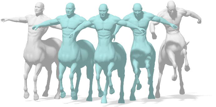
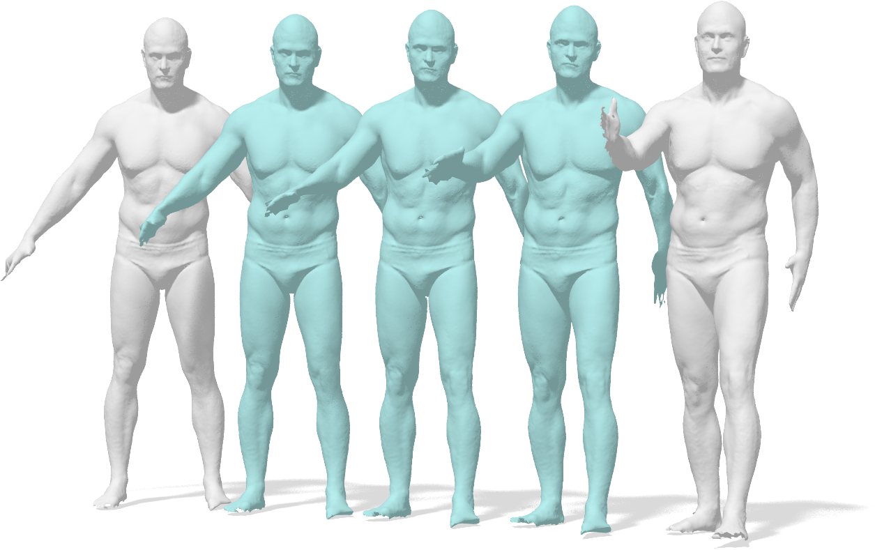
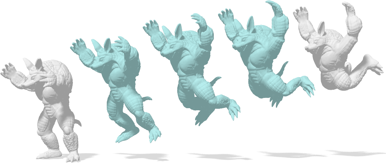
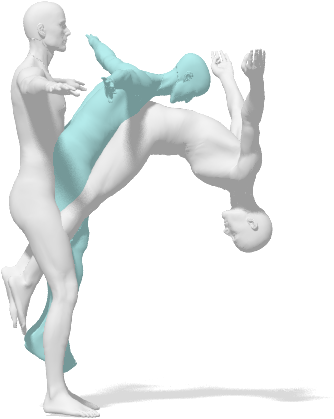
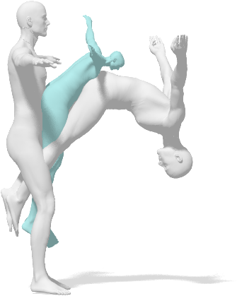
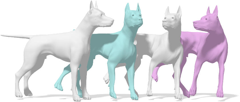
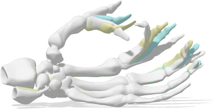
Given two input shapes we propose to compute a volume preserving deformation field by imposing a zero-divergence constraint. The resulting method alternates between optimizing the deformation field and calculating a correspondence for a small subset of vertices. (Left) Example of a deformation field in 3D. (Right) Our approach generates a continuous family of intermediate shapes along with a highly accurate correspondence. The input shapes are shown in white, intermediate shapes in blue and one extrapolation is shown in pink.
Divergence-Free Shape Interpolation and Correspondence
Abstract
We present a novel method to model and calculate deformation fields between shapes embedded in . Our framework combines naturally interpolating the two input shapes and calculating correspondences at the same time. The key idea is to compute a divergence-free deformation field represented in a coarse-to-fine basis using the Karhunen-Loéve expansion. The advantages are that there is no need to discretize the embedding space and the deformation is volume preserving. Furthermore, the optimization is done on downsampled versions of the shapes but the morphing can be applied to any resolution without a heavy increase in complexity. We show results for shape correspondence, registration, inter- and extrapolation on the TOSCA and FAUST Scan data sets.
{CCSXML}<ccs2012> <concept> <concept_id>10010147.10010371</concept_id> <concept_desc>Computing methodologies Computer graphics</concept_desc> <concept_significance>500</concept_significance> </concept> <concept> <concept_id>10010147.10010371.10010396.10010402</concept_id> <concept_desc>Computing methodologies Shape analysis</concept_desc> <concept_significance>500</concept_significance> </concept> </ccs2012>
\ccsdesc[500]Computing methodologies Computer graphics \ccsdesc[500]Computing methodologies Shape analysis
\printccsdesc1 Challenges in Shape Analysis
Handling non-rigidly deformed versions of a 3D shape is at the heart of numerous problems in computer vision and graphics ranging from shape comparison, information and style transfer to the automatic generation of new but meaningful shapes. In contrast to rigid shape registration which has six degrees of freedom, the problem of finding non-rigid deformations is rather ambiguous and the complexity of the optimization grows quadratically with the number of vertices in the input shapes.
While many of these problems are intrinsically related, most existing methods address them independently and do not generalize to a wider range of tasks. For example, having the same texture on both input shapes can help to find correspondences between these, while knowing the correspondence makes it easy to transfer the texture. Doing joint optimization can help to improve the performance in both tasks. Our approach combines shape registration, correspondence and interpolation – bringing different viewpoints to the same question of how to model non-rigid shape deformations.
Shape registration aims at finding a transformation of a shape that aligns its surface with another shape as closely as possible. This is trivial when the correspondence is already given, because then we can prescribe a deformation which aligns each point with its match . Vice versa, when two surfaces are aligned a correspondence can easily be found by searching for the nearest neighbor of each point in the embedding space. The shape interpolation problem addresses the task of finding a sequence of intermediate shapes between and such that is transformed into in a natural and continuous way. Most methods tackling this task assume they are given a perfect correspondence between the initial shapes but the existence of a smooth transition is actually a requirement for a good correspondence.
Many state-of-the-art correspondence methods can find fairly accurate matchings but they often rely on pointwise information like descriptor values or pairwise distances. While these are straightforward to compute, information about continuity is not encoded or increases the complexity of the optimization heavily. Consequently, outliers due to intrinsic symmetries or different sampling prevent a continuous morphing. In this work we will introduce a representation that can formulate both problems and makes a joint optimization possible.
2 Related Work
2.1 Deformation Fields
Deformation fields have a long history in image registration. Ashburner and colleagues made use of deformation fields for autonomous shape morphing [Ash07]. They consider temporally constant deformation fields offering limited flexibility to capture more complex deformations. Solving for a space and time dependent deformation field is a highly underdetermined problem. A remedy for this issue is provided by the geodesic shooting approach advocated by [MTY06] which only estimates the initial velocity field for each pixel and then how the velocity has to propagate in the image domain in order to preserve the kinetic energy and the momentum of the whole system. Further improvements of this framework were proposed in subsequent work, including a Gauss-Newton approach [AF11] and a particularly efficient adjoint calculation [VRRC12].
Closely related to our work is [vFTS06] in which the authors also model volume preserving shape deformations using divergence-free vector fields. Here, deformation fields are constructed from hand crafted templates which are meant to be used as interactive shape transformation tools.
It is often beneficial to have a probabilistic interpretation of deformation fields. This yields a comprehensive description with explicit schemata to impose uniformity on vector fields as well as a sound theoretical foundation. Such a model for image registration and 2D shape registration with a Gaussian process modeling of the correspondence mapping is proposed in [ALV08]. Further work [LJGV16, DGL∗17] specified how one can extend this approach to Gaussian processes on the surface of a three dimensional shape. The authors in [BHB00], [THB08], [ALV08] and [PDBS∗09] also model non-rigid transformations using a PCA type representation of permitted motions. Analogously, [MS10] and [MZT∗14] pursue a reproducing kernel Hilbert space approach to model the vector field interpolation. However, for all these references the respective vector fields are not defined on the whole embedding space surrounding the shapes but rather only at the elements of the considered point clouds and they do not admit an interpretation as a deformation field.
2.2 Shape Registration and Matching
Much work has been done in the direction of shape registration and matching and we would like to point the interested reader to in-depth surveys of these topics for an overview [vKZHCO11, SMFF07, TCL∗13]. Here we will focus on work that is directly related to our approach.
A popular line of work in shape matching is based on spectral decomposition of the surface Laplace-Beltrami operator [DK10]. This is popular because it reduces the dimensionality of the problem from the number of vertices to the number of basis functions chosen [OBCS∗12]. Nevertheless, extracting the correspondence from the low dimensional representation is still a complex problem and often retrieved solutions are noisy or hard to compute [RMC15]. We also use a spectral approach but, instead of a basis for functions on the surface, we represent deformation fields in the embedding space using the eigenfunctions of the standard Laplacian.
Methods based on Multi-Dimensional Scaling find correspondences by reembedding and then aligning shapes in a (possibly smaller) embedding space where the complexity is reduced [BBK06, ADK16]. [CK15] calculate a robust non-rigid registration based on Markov random fields but can not retrieve a continuous deformation. In [MS10] and [MZT∗14] the authors address the non-rigid registration problem by modeling one point cloud as a Gaussian mixture model. Moreover, they also determine the correspondences and point mappings in an alternating manner using a expectation maximization algorithm. This work is strongly related to our framework. Like our approach they directly model the correspondence mapping of all points as a Gaussian process type mapping. There also exist extensions of this method which additionally include descriptor values [MZY16, MJLL17].
2.3 Shape Interpolation
Although registration methods often compute a deformation between shapes, the focus is not on producing realistic intermediate shapes. Most methods realistically interpolating between shapes assume to be given a full correspondence in advance. [KMP07] interprets the solution to interpolation as geodesics in the pointwise shape space. [WBRS11] and [HRS∗16] model a space of shells with metrics induced by physical deformation energies in which geodesics or splines represent natural interpolations between shells. [VTSSH15] make real-time interpolation on a set of preprocessed, given shapes with arbitrary resolution possible.
[ACOL00] only needs a handful of correct correspondences to find a volume preserving deformation between two shapes but they require both to be segmented in compatible simplicial complexes. In [XZWB05] a dense deformation field similar to ours is calculated but the method depends on a consistent triangulation of the inputs. Other directions include taking user input to guide deformations in the right direction [VMW15] or rely on a known or learned model to generate new shapes [GCLX17].
3 Contribution
In the following, we will introduce a mathematical framework which allows to jointly tackle the problems of shape interpolation/extrapolation, shape registration and correspondence estimation. Our method solely operates on two given 3D point clouds and in particular requires no connectivity information like a mesh. We propose to estimate a smooth and volume preserving 3D deformation field prescribing a plausible interpolation of these input shapes. More specifically, we solve an initial value problem for determining the shape deformation. This framework allows us to incorporate physical assumptions about the deformation field. We suggest to impose volume preservation by enforcing zero divergence. More specifically, we represent the deformation field as the curl of a potential function and propose a natural coarse-to-fine basis representation of these potential functions. The initial value problem is then integrated by a Runge-Kutta scheme. We use an expectation maximization approach to simultaneously determine a subset of the unknown point-to-point correspondences and the optimal deformation field parameters. The objective is aligning two shapes with a preferably uniform deformation field. We demonstrate that the proposed framework can be used to create plausible shape interpolations and extrapolations in numerous experiments. Moreover, it provides a shape correspondence which compares to state-of-the-art correspondence methods.
4 Problem Formulation
This section gives an introduction into the problem we want to solve and the mathematical background we use in later sections.
4.1 Deformation field shape correspondences
Consider two discrete sets of points and contained in a compact domain . The points and are assumed to be uniformly sampled from the surface of two similar -dimensional shapes. The shape registration problem now addresses the task of aligning the point clouds and in a meaningful manner, such that similar regions of the two shapes are matched onto each other. In particular we are looking for a morphing , such that the mapped points fit to the shape .
Our approach chooses these mappings in such a way that they imitate plausible transformations in the real world. For this purpose we make some natural assumptions about the trajectories of the transformed points . For once we require the points of our shape to move smoothly over time. We would also like points in a certain neighborhood to shift in a uniform manner. This assumption yields to some extent that the determined correspondences are continuous. Moreover, the volume of shifted objects should remain the same. We therefore assume that every point moves according to the following initial value problem:
| (1) |
In this context is some fixed deformation field moving the point over time. In order to ensure a uniform movement of the samples the vector field has to be sufficiently smooth. We will even assume that , which yields the following well-known result:
Proposition 1
For a deformation field , the initial value problem (1) admits a solution on the compact domain and this solution is unique. Furthermore it is infinitely many times continuously differentiable
Proof 4.2.
As a consequence we can choose the correspondence mapping to be the solution operator of (1) evaluated at an arbitrary time . For convenience we choose :
| (2) |
The advantage of this framework is that it provides an intuitive notion of deformation when analyzing shape correspondences. Therefore, one does not only get a matching of two shapes but also all intermediate states constituting the underlying transformation. Those are typically more meaningful than merely performing linear interpolation between the initial and the final position of each point . Especially when looking at nearly isometric shapes having a continuous correspondence and a natural deformation are inherently connected and solving for both simultaneously improves the results considerably.
4.2 Divergence free deformations
Another convenient quality of the presented framework is that it enables us to incorporate assumptions about the deformation field into our model. One reasonable restriction arises from the mathematical investigation of fluid dynamics [CM93], namely the restriction to divergence free velocity fields:
| (3) |
It is well known that this local property confines the vector field in such a way, that it yields volume conservation over time for any considered part of the shape:
Proposition 4.3.
Proof 4.4.
This statement is a particular case of the result in [Tes12, Lemma 8.8].
Helmholtz’s theorem [Ari62] implies that any sufficiently smooth vector field on the compact domain can be decomposed into the sum of a curl free and a divergence free component. It furthermore provides us with an explicit construction of the divergence free component of any velocity field:
| (5) |
In this context is a potential field. This vector field arises from a construction in the Helmholtz decomposition and it typically depends on the considered vector field . Unfortunately constructing from is not straightforward and it is in general not computationally feasible. Therefore we allow the potential to be an arbitrary vector field. Then we can define to be its curl in analogy to (5). Either way we get a divergence free vector field due to the following basic property of the curl operator:
| (6) |
In the case of spatial dimensions the construction of in (5) admits the following form:
| (7) |
5 Method
Regarding relevant applications we will mainly restrict ourselves to the case of . However, extensions to higher dimensions or the 2D case are straightforward.
5.1 Spatial representation
We need to describe the velocity fields in a more tangible manner such that we obtain a computationally feasible method. The problem is that there are infinitely many choices for functions . The most straightforward approach is choosing a discretization of the embedding space, e.g. with a voxel grid. The potential and deformation fields can then be defined by assigning a three-dimensional vector to every voxel. The problem with this approach is that it has cubic complexity which becomes costly very fast. Furthermore, we do not get a spatially continuous deformation and loose volume conservation and other desirable properties as a consequence. In the following we will introduce a finite, linear basis for any velocity field on and derive a formulation to restrict it to only span smooth, divergence-free fields. The number of basis function can be adjusted for either speed or expressiveness.
The eigenfunctions of the Laplace-Beltrami operator are often used in shape analysis because of their useful properties like invariance to non-rigid deformations, smoothness and natural ordering. We use a similar basis for smooth, divergence-free vector fields in . Without loss of generality the considered domain is assumed to be a -dimensional cube and we translate and scale any shape to generously fit inside. We start with the eigenfunctions of the standard Laplacian on :
| (8) |
This basis of eigenfunctions is ordered such that the eigenvalues are descending. Furthermore, we require the Laplacian to admit Dirichlet boundary conditions . The can be determined analytically and they are exactly the elements of the Fourier basis:
| (9) |
These functions now form an orthonormal basis wrt. the norm. The eigenvalue of corresponding to the eigenfunction is the following:
| (10) |
We can now map the potential basis to the velocity field to obtain a feasible description . For this purpose we directly insert the basis elements from (9) into the places of the components of in (5). Due to the linearity of the curl operator this can be done for every entry of at a time, see (7) for . Overall, we obtain a basis of the velocity field . In the 3D case it is explicitly defined as:
| (11) |
In this context the basis elements are again sorted according to the eigenvalues of the corresponding in descending order. Note that there are in general multiple basis functions for each eigenvalue . This yields a feasible description of the velocity field by computing as a linear combination of the first basis elements:
| (12) |
The coefficients can be defined as random variables with a Gaussian prior distribution . This assumption yields a probability distribution over all admissible deformation fields which we will use later to obtain the optimization energy function. The weights are constructed from the eigenvalues in the following manner:
| (13) |
Intuitively this kind of weighting promotes a damping of the high frequency components of and therefore yields a uniform vector field, because the coefficients are sampled with a smaller variance . This also justifies the truncation in (12), because the weights corresponding to high frequency basis elements are insignificantly small anyway. The mathematical background of the sampling approach in (12) is provided by the Karhunen-Loève expansion [Sul15, Ch. 11] which is an extension of the principal component analysis (PCA) for more general vector spaces.
The Dirichlet boundary conditions automatically guarantee that there is no flow out of the domain , in the sense that the components of are orthogonal to the outer normals at the boundary . This can be easily verified for the case by computing the basis elements (11) inserting (9), but we refrain from proving this property here. It also becomes obvious by looking at instances of the velocity basis functions in Figure 2.
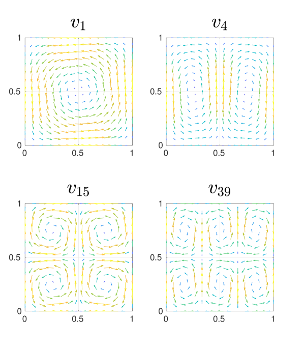
Our representation of the velocity field has several beneficial properties. First of all, it can be evaluated at any point in the domain and we do not need to introduce a spatial discretization. We will use this in our experiments to make our method applicable to very high resolution shapes. Secondly, the particular weighting of the summands and the truncation in (12) induces an inbuilt low-pass filtering which produces smooth deformations because it favors the low frequency basis elements.
Classical shape registration methods like the iterative closest point (ICP) algorithm [BM92] determine a rigid transformation between two shapes. Interestingly, our approach can be interpreted as a direct extension of these methods. The deformation fields corresponding to translations and rotations are divergence free and uniform, and therefore, contained in our framework by design. This becomes even clearer when the basis function in Figure 2 is examined. It is fairly similar to a rotation around the axis. This especially holds near the center of the domain and deteriorates at its boundary . Actually it is fairly straightforward to verify, that this equivalence holds up to first order around the center. The basis elements and express rotations around the and axis in a similar way. The considerations in this subsection raise the question whether a cubic domain is the best choice for our purposes. Following the work in [ZB07], [ZB08] we could pursue our approach in a spherical domain. This would lead to more complex basis functions but the first three eigenfunctions would span the space of rotations without undesirable artifacts at the boundaries of the domain. Although this would be a nice theoretical property we refrain from using these basis functions here due their complex structure, especially because this does not lead to a quantifiable improvement of our method.
5.2 Temporal discretization
In order to evaluate the correspondence mapping in (2) we have to solve the initial value problem (1) by a numerical integration scheme. The simplest choice in this context is the explicit Euler method. However, we decided to use a second order Runge-Kutta method [GH10, Ch. 9], because it has a significantly higher accuracy and therefore enables us to choose a coarser discretization. We subdivide the time space in an equidistant grid with intervals and set the step size . This yields the following explicit iteration scheme:
| (14) |
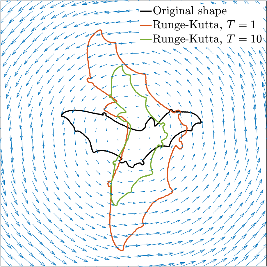
We typically choose in our experiments. In general, we have to make a trade off between runtime and accuracy when selecting a proper number of steps . We commonly also get meaningful transformations if we choose to be small but we might loose some key properties of our framework like the volume preservation. This effect is illustrated in Figure 3 for the 2D shape of a bat transformed by a 90 degree rotation around the center. Note that the deformation field corresponding to this transformation is actually not contained in our framework due to our choice of domain and boundary conditions, see discussion in the previous subsection. If for this setup we now choose too few time steps , the shape shifts outward and the area expands. On the other hand, this effect becomes insignificantly small if we choose .
5.3 Optimization
In the previous sections we derived a coherent description of shape morphing using volume preserving deformation fields. We can now use this framework to construct an algorithm that matches two given point clouds and while at the same time computing plausible interpolated shapes. In order to do that we need to simultaneously optimize for the deformation fields and the unknown correspondences. We encode the latter using a soft correspondence matrix . High values of indicate a high correspondence probability for the point pair . Moreover, we use the coefficients to represent the deformation fields which according to (12) are completely determined by .
Similar to [MS10] and [MZT∗14] we address shape registration in a probabilistic manner. We interpret the point cloud as a Gaussian mixture model with the means located at the shifted points and the covariance for some . This enables us to simultaneously determine the deformation field coefficients and the correspondences by applying an expectation maximization approach.
Only using Euclidean distance as the measure of similarity between points suffices to capture rigid deformations but this fails if source or target undergo large non-rigid deformations and often leads to incorrect local optimums. Therefore, we incorporate point-wise feature descriptors in our model. They can account for large scale deformations but also encode information about fine scale structures which steers the optimization towards the right optimum. Specifically, we use the SHOT descriptor [TSS10] with the distance function on the sets of points and . The standard GMM formulation only uses the Euclidean distance of the shifted point and . We want to use a combination of both, therefore we will define the distance of and to be:
| (15) |
Here, is the mean distance of a metric regarding all point pairs in and and the factor at is used to ensure that both metrics have a comparable scaling. Note that is a metric on the point clouds and as a positive combination of metrics. Using this notion of distance, we can specify how to update the soft correspondences using the current estimate of the deformation field parameters . This corresponds to the E step of the expectation maximization algorithm:
| (16) |
In the context of (12) it was mentioned that the prior of the coefficients is a Gaussian distribution , where . Together with the GMM assumption for the shape we can construct the following energy function for the M step:
| (17) |
The function is the Huber loss [Hub64]:
| (18) |
In our evaluations, we choose the outer slope as . Note that the Huber loss does not directly arise from the standard GMM formulation, but it admits another probabilistic interpretation as an additive mixture of Huber density functions. It also helps to account for outliers and makes the deformation field estimation more robust in general.
In our experiments we apply a Gauss-Newton type approach to minimize the energy in (17). This results in an iterative method similar to the Levenberg-Marquardt algorithm [Lev44]. The overall expectation maximization algorithm now alternates between computing the weights according to (16) and performing one Gauss-Newton update step to obtain . To initialize the algorithm we usually set the deformation field to be zero .
6 Experiments
We perform experiments for several applications including shape matching and interpolation to show that our method is general and flexible. Although we handle shapes with up to and more vertices, the computation of the deformation field is always done on a downsampled version with vertices and then applied to the full resolution. We use Euclidean farthest point sampling. When downsampling the subset should include all relevant fine scale structures in order for the deformation field to move these correctly but we found sufficient for all our applications. As a preprocessing step, we align the shapes using PCA and shift them such that the empirical mean of the point clouds corresponds to the middle of the domain. When averaging over all experiments presented here, our algorithm takes about seconds to compute all correspondences for one pair of shapes. Due to our a priori downsampling the runtime is pretty consistent and almost independent of the number of vertices. All experiments were performed with MATLAB on a system with an Intel Core i7-3770 CPU clocked at 3.40GHz, 32 GB RAM and a GeForce GTX TITAN X graphics card running a recent Linux distribution. In all our experiments, we solely operate on the raw shape data and in particular do not need any ground truth correspondences.
6.1 Matching
We verify our method using the TOSCA dataset [BBK08] which contains 76 triangular meshes. The dataset is divided into classes of humans and animals with several poses each and known intraclass correspondences.
We set the hyperparameters and choose basis functions for the deformation field. Because only contains correspondences, we perform a nearest-neighbor search with the metric (15) to obtain a dense mapping. The evaluation is done with the Princeton benchmark protocol [KLF11]. Given the ground-truth match , the error of the calculated match is given by the geodesic distance between and normalized by the diameter of .
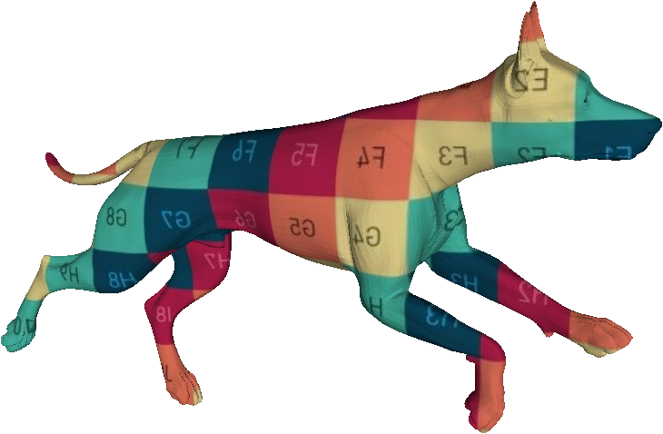
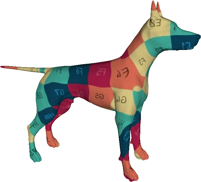
We plot cumulative curves showing the percentages of matches that are below an increasing threshold. As zero is the value for ground-truth matches, the ideal curve would be constant at . See Figure 4 for our results and Figure 5 for an example matching.
6.2 Registration
We apply our framework to the FAUST dataset [BRLB14], which contains data from scans of real humans with different poses. Each of these shapes has approximately vertices and some of them are severely affected by topological noise. We set , and we use a temporal discretization of steps. Again we match the null shape of every person to all its other poses. In Figure 6 we display the surface distance of the morphed shapes to the goal shape for some examples.
6.3 Shape Interpolation
In comparison to other shape matching approaches, our setup models deformations in a comprehensive manner. It has a built in description of the actual transformation shapes undergo over time to morph into one another. Therefore it produces interpolated shapes a byproduct.
In some sense, our approach can be considered to be the extension of other shape registration methods based on a Gaussian mixture model representation of a point cloud [MS10], [MZT∗14]. These particular methods correspond to our approach, if we choose to integrate the initial value problem (1) with the forward Euler scheme and time step. In particular this leads to a linear dependence of the quantity on the unknowns and the mapping for this case admits the following form:
| (19) |
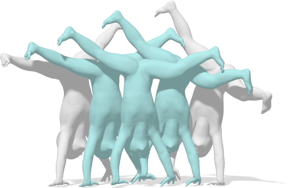
As a consequence the shift (19) of each point over time yields affine linear trajectories. Therefore the intermediate configurations are equivalent to a pointwise linear interpolation. In contrast to this our method produces point trajectories which correspond to solutions of the ODE (1). We can now evaluate those at an intermediate time . Three examples of this qualitative evaluation were already displayed in Figure 1, another one is provided in 7.
In comparison to our approach linear interpolation distorts the shapes considerably, see Figure 8. It also changes the size of certain parts of the shape which is inconsistent with transformations in the real world. In contrast to this our method is locally volume preserving. Nevertheless, it can still stretch and bend the shapes. Therefore, it is suitable for modeling shape morphing for rigid, as well as elastic objects. Linear interpolation performs especially bad if the considered transformations include large rotations.
Extrapolation
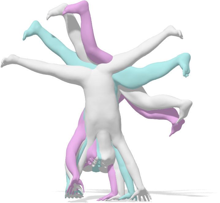
According to (1) the deformation field is independent of the time which makes the ODE autonomous. Therefore, we can also use the computed vector field to determine the solutions of this initial value problem at times which produces extrapolated shapes, see Figure 9. It is obviously an underdetermined task and it is hard to evaluate quantitatively. Nevertheless the extrapolation shapes our method produces are in many cases quite realistic for moderate time spans . Another example is displayed in Figure 10. We observe that the speed of the extrapolated shapes seems to slow down after a certain timespan, especially when the shape is moving in previously unoccupied space. For the optimization there is simply no incentive to impose any particular movement on these parts of the domain . However, the volume preservation and uniformity assumption infer to the algorithm that an extension of the previous movement to some extend is desirable. Overall the resulting shapes are visually appealing and not too severely affected by distortions.
7 Conclusion
We presented a novel method solving the shape correspondence problem while simultaneously computing a smooth, volume preserving deformation field between the input shapes. Furthermore, this deformation can be used to efficiently calculate plausible interpolated shapes between the inputs at any intermediate point in time. The method consists of two parts, the first is the optimization of the deformation field using an expectation maximization approach and the second applies the deformation to the input shapes using a Runge-Kutta scheme. The big advantage is that a subsampling with around vertices is sufficient to obtain the deformation field defined in the continuous embedding space due to our choice of basis. Therefore, the result can be applied to any resolution mesh without slowing the optimization.
We show quantitative results for shape correspondence and registration that can compare to state-of-the-art methods for these specific tasks and examples of shape interpolation and extrapolation that arise naturally from our pipeline.
7.1 Limitations
Due to our choice of basis the deformation field is forced to be volume preserving. This makes sense in applications with the same object but prevents inter-object matchings - for example between two humans with different body shapes.
For the same reason, our method has problems with topological changes. According to Proposition 4.3 the volume preservation property applies to every subregion of the domain , including the intermediate space between parts of the shape. Therefore, separating two touching parts (for example two hands) is in theory possible but requires many high frequency deformation basis elements which makes the optimization costly.
Since there is not one unique, volume preserving deformation between two shapes, our interpolation is not guaranteed to be as-rigid-as-possible which is plausible in many applications. If the displacement is spatially far, we might end up with squeezed intermediate states that are volume preserving but are affected by undesirable distortions.
The assumption of (1) being autonomous can also be problematic, if different parts of the shape move through the same region of the embedding space in a contradictory manner. One example for this is a hand closing to a fist. At first the index and middle finger occupy parts of the embedding space before the thumb moves in the same area but in a different direction. See Figure 11. A possible remedy for this problem is making the deformation fields time dependent.
7.2 Future Work
Right now, the method will always find a solution that is globally volume preserving. This allows to find good deformations fields in the case of severe non-rigid deformations but is not applicable to partial data. In the future, we want to extend this method to work on real scans, for example from the Kinect, which naturally only show partial shapes by making the deformation only locally volume preserving. This might also help with the separation of close parts and handling non volume preserving deformations like style or class changes. Furthermore, we only calculate one time independent field for the entire deformation which means mass at one spatial point always needs to move in the same direction, even at a later time step. This restricts the complexity of the deformations that our method can handle, especially for large-scale motions over a longer period of time. It also leads to problems when non-matching parts of the input shapes overlap in the initialization. Future versions should allow more flexible types of deformation fields to extend it to a broader range of applications. We could for example associate different parts of the shape with different deformations fields or let them vary over time to address more difficult tasks.
References
- [ACOL00] Alexa M., Cohen-Or D., Levin D.: As-rigid-as-possible shape interpolation. In Proceedings of the 27th Annual Conference on Computer Graphics and Interactive Techniques (2000), SIGGRAPH ’00, pp. 157–164.
- [ADK16] Aflalo Y., Dubrovina A., Kimmel R.: Spectral generalized multi-dimensional scaling. IJCV 118, 3 (2016), 380–392.
- [AF11] Ashburner J., Friston K. J.: Diffeomorphic registration using geodesic shooting and gauss–newton optimisation. NeuroImage 55, 3 (2011), 954–967.
- [aim] AIM@SHAPE repository. http://visionair.ge.imati.cnr.it:8080/ontologies/shapes/viewgroup.jsp?id=657-Armadillo_1.
- [ALV08] Albrecht T., Lüthi M., Vetter T.: A statistical deformation prior for non-rigid image and shape registration. 2008 IEEE Conference on Computer Vision and Pattern Recognition (2008), 1–8.
- [Ari62] Aris R.: Vectors, tensors, and the basic equations of fluid mechanics. Englewood Cliffs, N.J., Prentice-Hall, 1962.
- [Ash07] Ashburner J.: A fast diffeomorphic image registration algorithm. Neuroimage 38, 1 (2007), 95–113.
- [BBK06] Bronstein A. M., Bronstein M. M., Kimmel R.: Generalized multidimensional scaling: a framework for isometry-invariant partial surface matching. PNAS 103, 5 (2006), 1168–1172.
- [BBK08] Bronstein A. M., Bronstein M. M., Kimmel R.: Numerical geometry of non-rigid shapes. Springer, 2008. http://tosca.cs.technion.ac.il/book/resources_data.html.
- [BHB00] Bregler C., Hertzmann A., Biermann H.: Recovering non-rigid 3d shape from image streams. Proceedings IEEE Conference on Computer Vision and Pattern Recognition 2 (2000), 690–696.
- [BM92] Besl P. J., McKay N. D.: Method for registration of 3-d shapes. In Sensor Fusion IV: Control Paradigms and Data Structures (1992), vol. 1611, International Society for Optics and Photonics, pp. 586–607.
- [BRLB14] Bogo F., Romero J., Loper M., Black M. J.: FAUST: Dataset and evaluation for 3D mesh registration. In Proceedings IEEE Conf. on Computer Vision and Pattern Recognition (CVPR) (Piscataway, NJ, USA, June 2014), IEEE.
- [CK15] Chen Q., Koltun V.: Robust nonrigid registration by convex optimization. In IEEE International Conference on Computer Vision (ICCV) (2015), pp. 2039–2047.
- [CM93] Chorin A. J., Marsden J. E.: A Mathematical Introduction to Fluid Mechanics. Springer, 1993.
- [DGL∗17] Dölz J., Gerig T., Lüthi M., Harbrecht H., Vetter T.: Efficient computation of low-rank gaussian process models for surface and image registration.
- [DK10] Dubrovina A., Kimmel R.: Matching shapes by eigendecomposition of the laplace-beltrami operator.
- [GCLX17] Gao L., Chen S.-Y., Lai Y.-K., Xia S.: Data-driven shape interpolation and morphing editing. Comput. Graph. Forum 36 (2017), 19–31.
- [GH10] Griffiths D., Higham D. J.: Numerical Methods for Ordinary Differential Equations. Springer, 2010.
- [HRS∗16] Heeren B., Rumpf M., Schröder P., Wardetzky M., Wirth B.: Splines in the space of shells. Computer Graphics Forum 35, 5 (2016), 111–120.
- [Hub64] Huber P. J.: Robust estimation of a location parameter. Annals of Statistics 53, 1 (1964), 73–101.
- [KLF11] Kim V. G., Lipman Y., Funkhouser T. A.: Blended intrinsic maps. Trans. Graphics 30, 4 (2011).
- [KMP07] Kilian M., Mitra N. J., Pottmann H.: Geometric modeling in shape space. In ACM Transactions on Graphics (TOG) (2007), vol. 26, ACM, p. 64.
- [Lev44] Levenberg K.: A method for the solution of certain non-linear problems in least squares. Quarterly of Applied Mathematics 2, 2 (1944), 164–168.
- [LF09] Lipman Y., Funkhouser T.: Möbius voting for surface correspondence. In Trans. Graphics (2009), vol. 28, p. 72.
- [LJGV16] Lüthi M., Jud C., Gerig T., Vetter T.: Gaussian process morphable models. IEEE Transactions on Pattern Analysis and Machine Intelligence 99 (2016).
- [LSLCO05] Lipman Y., Sorkine O., Levin D., Cohen-Or D.: Linear rotation-invariant coordinates for meshes. In ACM Transactions on Graphics (TOG) (2005), vol. 24, ACM, pp. 479–487.
- [MJLL17] Ma J., Jiang J., Liu C., Li Y.: Feature guided gaussian mixture model with semi-supervised em and local geometric constraint for retinal image registration. Information Sciences 417 (2017), 128–142.
- [MS10] Myronenko A., Song X.: Point set registration: Coherent point drift. IEEE Transactions on Pattern Analysis and Machine Intelligence 32, 12 (2010), 2262–2275.
- [MTY06] Miller M. I., Trouvé A., Younes L.: Geodesic shooting for computational anatomy. Journal of mathematical imaging and vision 24, 2 (2006), 209–228.
- [MZT∗14] Ma J., Zhao J., Tian J., Yuille A. L., Tu Z.: Robust point matching via vector field consensus. IEEE Transactions on Image Processing 23, 4 (2014), 1706–1721.
- [MZY16] Ma J., Zhao J., Yuille A. L.: Non-rigid point set registration by preserving global and local structures. IEEE Transactions on image Processing 25, 1 (2016), 53–64.
- [OBCS∗12] Ovsjanikov M., Ben-Chen M., Solomon J., Butscher A., Guibas L.: Functional maps: a flexible representation of maps between shapes. ACM Transactions on Graphics (TOG) 31, 4 (2012), 30.
- [PDBS∗09] Paladini M., Del Bue A., Stosic M., Dodig M., Xavier J., Agapito L.: Factorization for non-rigid and articulated structure using metric projections. 2898–2905.
- [Ral] Ralph R.: MPEG-7 Core Experiment CE-Shape-1 Test Set. http://www.dabi.temple.edu/~shape/MPEG7/dataset.html.
- [RBW∗14] Rodola E., Bulo S. R., Windheuser T., Vestner M., Cremers D.: Dense non-rigid shape correspondence using random forests. In IEEE Conference on Computer Vision and Pattern Recognition (CVPR) (2014).
- [RMC15] Rodolà E., Moeller M., Cremers D.: Point-wise Map Recovery and Refinement from Functional Correspondence. In Vision, Modeling and Visualization (2015), The Eurographics Association.
- [SMFF07] Salvi J., Matabosch C., Fofi D., Forest J.: A review of recent range image registration methods with accuracy evaluation. Image Vision Comput. 25, 5 (2007), 578–596.
- [Sul15] Sullivan T. J.: Introduction to Uncertainty Quantification. Springer, 2015.
- [TCL∗13] Tam G. K. L., Cheng Z.-Q., Lai Y.-K., Langbein F. C., Liu Y., Marshall D., Martin R. R., Sun X.-F., Rosin P. L.: Registration of 3d point clouds and meshes: A survey from rigid to nonrigid. IEEE Transactions on Visualization and Computer Graphics 19, 7 (July 2013), 1199–1217.
- [Tes12] Teschl G.: Ordinary Differential Equations and Dynamical Systems. AMS, 2012.
- [THB08] Torresani L., Hertzmann A., Bregler C.: Nonrigid structure-from-motion: estimating shape and motion with hierarchical priors. IEEE Transactions on Pattern Analysis and Machine Intelligence 30, 5 (2008), 878–892.
- [TSS10] Tombari F., Salti S., Stefano L. D.: Unique signatures of histograms for local surface description. In Proceedings ECCV 16, 9 (2010), 356–369.
- [vFTS06] von Funck W., Theisel H., Seidel H.-P.: Vector field based shape deformations. In ACM Transactions on Graphics (TOG) (2006), vol. 25, ACM, pp. 1118–1125.
- [vKZHCO11] van Kaick O., Zhang H., Hamarneh G., Cohen-Or D.: A survey on shape correspondence. Computer Graphics Forum 30, 6 (2011), 1681–1707.
- [VLB∗17] Vestner M., Lähner Z., Boyarski A., Litany O., Slossberg R., Remez T., Rodolà E., Bronstein A. M., Bronstein M. M., Kimmel R., Cremers D.: Efficient deformable shape correspondence via kernel matching. In International Conference on 3D Vision (3DV) (October 2017).
- [VMW15] Vaxman A., Müller C., Weber O.: Conformal mesh deformations with mÖbius transformations. ACM Trans. Graph. 34, 4 (July 2015), 55:1–55:11.
- [VRRC12] Vialard F.-X., Risser L., Rueckert D., Cotter C. J.: Diffeomorphic 3d image registration via geodesic shooting using an efficient adjoint calculation. International Journal of Computer Vision 97, 2 (2012), 229–241.
- [VTSSH15] Von-Tycowicz C., Schulz C., Seidel H.-P., Hildebrandt K.: Real-time nonlinear shape interpolation. ACM Trans. Graph. 34, 3 (May 2015), 34:1–34:10.
- [WBRS11] Wirth B., Bar L., Rumpf M., Sapiro G.: A continuum mechanical approach to geodesics in shape space. International Journal of Computer Vision 93, 3 (Jul 2011), 293–318.
- [XZWB05] Xu D., Zhang H., Wang Q., Bao H.: Poisson shape interpolation. In Proceedings of the 2005 ACM Symposium on Solid and Physical Modeling (2005), pp. 267–274.
- [ZB07] Zhao C., Burge J. H.: Orthonormal vector polynomials in a unit circle, part i: basis set derived from gradients of zernike polynomials. Opt. Express 15, 26 (2007), 18014–18024.
- [ZB08] Zhao C., Burge J. H.: Orthonormal vector polynomials in a unit circle, part ii: completing the basis set. Opt. Express 16, 9 (2008), 6586–6591.
- [ZSCO∗08] Zhang H., Sheffer A., Cohen-Or D., Zhou Q., Van Kaick O., Tagliasacchi A.: Deformation-driven shape correspondence. In Computer Graphics Forum (2008), vol. 27, Wiley Online Library, pp. 1431–1439.