Reconciling low multipole anomalies and reheating in single field inflationary models

Abstract

Reheating phase of inflationary Universe can be modeled by parameters $T_{\text{reh}}$, $\bar{w}_{\text{reh}}$ and $N_{\text{reh}}$, which can be constrained by the scalar spectral amplitude $A_{s}$ and the scalar spectral index $n_{s}$. On the other hand the low multipole anomalies in the CMB can be modeled by suitable features in the inflaton potential. We show that the parameters of these features in the inflaton potential provide additional constraints on the reheating parameters. For several single field models we find that the reheating parameters are substantially more constrained by the requirement of compatibility with the proposed explanation for low multipole anomalies.

1 Introduction

Slow-roll inflation [1, 2, 3, 4, 5, 6, 7] predicts nearly scale invariant primordial power spectrum [8, 9, 10, 11, 12] that provides a good fit to the recent cosmic microwave background (CMB) data [13, 14, 15, 16, 17, 18, 19, 20, 21, 22, 23, 24]. The inflationary phase terminates by ‘reheating’  phase [25, 26, 27, 28, 29, 30, 31] so that the Universe subsequently evolves according to the hot big-bang model [32, 33]. The physics of reheating phase is completely undetermined and there are no direct observational data available, so far. However, indirect bounds can be obtained for the temperature at the end of the reheating ($T_{\text{reh}}$), the equation of state parameter, $w$, during reheating ($w_{\text{reh}}$) and the duration of reheating ($N_{\text{reh}}$) from recent CMB data.

Since slow roll inflation producing nearly scale invariant perturbations can be considered to have terminated if $w$ attains $w>-\frac{1}{3}$, it is convenient to assume that $w_{\text{reh}}$ = $-\frac{1}{3}$ at the beginning of the reheating. After the reheating era, $w$ is expected to be $\frac{1}{3}$, in order to make the Universe radiation dominated. Nevertheless, the allowed range of $w$ during the reheating is considered to be $-\frac{1}{3}\leq w_{\text{reh}}\leq 1$ in various scenarios. On the other hand, the lower and upper bounds of $T_{\text{reh}}$ are 10^-2 GeV (the big-bang nucleosynthesis (BBN) temperature) [34] and 10¹⁶ GeV (inflation energy scale) respectively.

The relation between reheating and inflationary parameters can be obtained by considering the evolution of observable cosmological scales from the time of Hubble crossing during inflation to present time [35, 36, 37, 32]. For single-field inflationary models, we can derive relations among $T_{\text{reh}}$, $N_{\text{reh}}$, $w_{\text{reh}}$, the scalar power spectrum amplitude ($A_{s}$) and the scalar spectral index $n_{s}$. In addition, CMB data is helpful in obtaining the constraints on $T_{\text{reh}}$ and $N_{\text{reh}}$ [38, 36, 39, 40, 32, 37, 41] .

The nearly scale invariant primordial power spectrum provides a good fit to the CMB data, and lends strong support to the essential paradigm of inflation. However at lower multipoles, specifically around $\ell={\bf{22}}$ and $\bf{40}$, the data points lie outside the cosmic variance associated with the power law primordial spectrum. It indicates that certain non-trivial inflationary dynamics are possible. If not of a completely accidental origin, the outlying data points could be important phenomenological inputs to deducing ancillary details of the inflationary model. There have been constant efforts [42, 43, 44, 45, 46, 47, 48, 49, 50] to reconstruct the primordial power spectrum from the CMB anisotropies in a model independent way.

The consideration of a burst of oscillations in the primordial power spectrum leads to a good fit to the CMB angular power spectrum, particularly around $\ell=\bf 22$ and 40 multipole moments [51, 52, 53]. In order to generate these oscillations in the primordial power spectrum, one has to consider a short period of deviation from slow-roll inflation [54, 55]. This deviation can be obtained by introducing a step in the inflaton potential [56, 17, 57, 58, 59, 60, 61, 62]. A step with suitable height and width at a particular location of the inflationary potential has resulted in a better fit to the CMB data near the multipole $\ell={\bf 22}$. In this paper we show that the generic relation between late time observables and reheating phase in a single field inflation can be strengthened by also demanding successful explanation of the low multipole anomalies. The link is the specific position of the inflaton in the course of its slow roll, $\phi_{k}/M_{Pl}$, at which it encounters the step in the potential. We obtain constraints on the reheating predictions of several inflationary models by using the location of the step in the inflaton potential as obtained in ref. [51]. The investigation can be extended easily to other models, as will be done in a future publication.

The article is organized as follows: Sec. 2 deals with the slow-roll inflation and its predictions. In Sec. 2, we derive the expressions for $T_{\text{reh}}$ and $N_{\text{reh}}$ as functions of $\bar{w}_{\text{reh}}$ and the inflationary parameters ($\Delta N_{k}$ and $V_{\text{end}}$) to be described there. The expressions for $T_{\text{reh}}$ and $N_{\text{reh}}$ are derived as a function of the scalar spectral index $n_{s}$ for different single field inflationary models in Sec. 3. In addition, the observational bounds on inflationary models and reheating parameters are discussed for large field, small field (hilltop) and Starobinsky model by using Planck 2015 data [23, 24]. In Sec. 4, the effect of considering a step in the inflaton potential and its consequences on the constraints on reheating parameters are detailed. Sec.5 contains the conclusions.

We work with $\hbar=c=1$ units and the following values are used. $M_{\text{Pl}}=\sqrt{\frac{1}{8\pi G}}=2.435\times 10^{18}\text{GeV}$ is the reduced Planck mass and the redshift of last scattering surface is $z_{ls}=1100$. The $z_{\text{eq}}=3365$ is the redshift of matter radiation equality and the present value of the Hubble parameter $H_{0}=100h$ km $\text{s}^{-1}\text{Mpc}^{-1}$ with $h=0.68$ [23, 24].

2 Reheating parameters in slow-roll models

We consider the inflaton $\phi$ governed by a potential $V(\phi)$ undergoing slow roll evolution with parameters $\epsilon$ and $\eta$, resulting in scalar curvature power spectrum $P_{\zeta}(k)$ and tensor power spectrum $P_{h}(k)$ as a function of the Fourier transform variable $k$ of the argument of the spatial correlation functions, with corresponding indices $n_{s}-1$ and $n_{T}$. The details of the definitions and notation are standard [63], and can be found also in the references [12, 64, 7]. We shall use $A_{s}$ and $A_{T}$, the amplitude of scalar and tensor power spectra at the pivot scale $k_{*}$ as used by Planck collaboration, $\frac{k_{*}}{a_{0}}=0.05\text{Mpc}^{-1}$. For $k=k_{*}$, these amplitudes are given in terms of $H_{*}$ as

$$A_{T}=P_{h}(k_{*})=\frac{2H_{*}^{2}}{\pi^{2}M_{\text{Pl}}^{2}},\hskip 28.45274ptA_{s}=P_{\zeta}(k_{*})=\frac{H_{*}^{2}}{8\pi^{2}M_{\text{Pl}}^{2}\epsilon_{*}}.$$ (2.1)

In terms of the slow-roll parameters $\epsilon$ and $\eta$, the tensor to scalar ratio $r$, the scalar spectral index $n_{s}$ and the tensor spectral index $n_{T}$ satisfy the relations

$$r=16\epsilon,\hskip 28.45274ptn_{s}=1-6\epsilon+2\eta,\hskip 28.45274ptn_{T}=-2\epsilon.$$ (2.2)

The total number of e-foldings, $N_{T}$, is defined as the logarithm of the ratio of the scale factor at the final time $t_{e}$ to it’s value at initial time $t_{i}$ of the era of inflation.

$$N_{T}\equiv\ln\frac{a(t_{e})}{a(t_{i})}=\int_{t_{i}}^{t_{e}}{Hdt}=\int_{\phi_{i}}^{\phi_{\text{end}}}{\frac{H}{\dot{\phi}}d\phi}=\frac{1}{M_{\text{Pl}}}\int^{\phi_{i}}_{\phi_{\text{end}}}{\frac{1}{\sqrt{2\epsilon}}d\phi}.$$ (2.3)

Where $\phi_{i}$ and $\phi_{\text{end}}$ are the initial and final values of the inflaton field $\phi$ and $\epsilon$ is the slow-roll parameter defined as $\epsilon=-\dot{H}/H^{2}=\dot{\phi}^{2}/(2H^{2}M_{\mathrm{Pl}}^{2})$. Likewise, given a mode $k$, the number of e-foldings between the time when it crosses the Hubble horizon and the end of inflation is given by

$$\Delta N_{k}=\int_{\phi_{k}}^{\phi_{\text{end}}}{\frac{H}{\dot{\phi}}d\phi}=\frac{1}{M_{\text{Pl}}}\int^{\phi_{k}}_{\phi_{\text{end}}}{\frac{1}{\sqrt{2\epsilon}}d\phi},$$ (2.4)

where $\phi_{k}$ is the value of the inflaton field at the time of Hubble crossing of the scale k. For the slow-roll approximation i.e., $V(\phi)\gg\dot{\phi}^{2}$ and $\ddot{\phi}\ll 3H\dot{\phi}$ the eq. (2.4) becomes

$$\Delta N_{k}\approx\frac{1}{M_{\text{Pl}}^{2}}\int_{\phi_{\text{end}}}^{\phi_{k}}{\frac{V}{V^{\prime}}d\phi}.$$ (2.5)

We shall also be interested in the situation where the slow roll condition is briefly violated. This happens when the inflaton negotiates the step in the potential. However for a small enough step, $\ddot{\phi}$ becomes appreciable only briefly and the kinetic energy $\frac{1}{2}{\dot{\phi}}^{2}$ does not grow appreciably [58, 65]. The brief departure from slow roll can be accounted for by an additional quantity $\Delta N_{\mathrm{step}}$ which can be shown to remain negligible compared to the main value of interest $\Delta N_{k}$. We demonstrate this in detail in Appendix A.

We now turn to relating the observed wavenumber of any physical scale today $\frac{k}{a_{0}}$, to its value at the time of Hubble crossing during inflation $\frac{k}{a_{k}}$. This can be obtained as

$$\frac{k}{a_{k}} = \frac{k}{a_{0}}\frac{a_{0}}{a_{k}},$$ (2.6)

$$= \frac{k}{a_{0}}\frac{a_{0}}{a_{\text{eq}}}\frac{a_{\text{eq}}}{a_{\text{reh}}}\frac{a_{\text{reh}}}{a_{\text{end}}}\frac{a_{\text{end}}}{a_{k}}.$$

Here $a_{k}$, $a_{\text{eq}}$ and $a_{0}$ represent the value of scale factor at the time of Hubble crossing, matter radiation equality and at present time respectively. The somewhat ill defined but physically significant epochs $a_{\text{end}}$, $a_{\text{reh}}$ represent end of inflation and the end of reheating respectively. For convenience one also introduces

$$N_{\text{reh}}\equiv\ln\left(\frac{a_{\text{reh}}}{a_{\text{end}}}\right)\qquad\textrm{and}\qquad\Delta N_{k}\equiv\ln\left(\frac{a_{\text{end}}}{a_{k}}\right)$$ (2.7)

in line with the number of e-foldings. The dynamic quantity $\Delta N_{k}$ represents the number of e-folds remaining after the scale $k$ has crossed the Hubble radius during inflation. The $a_{\text{reh}}$ demarkates successful return to a radiation dominated Universe. Hence the $N_{\text{reh}}$ encodes both, an epoch of preheating [66, 29, 67, 68, 69, 70] as well as a subsequent thermalization process. Subsequent evolution of the Universe governed by an energy density

$$\rho_{\text{reh}}=\frac{\pi^{2}}{30}g_{\text{reh}}T_{\text{reh}}^{4},$$ (2.8)

where $T_{\text{reh}}$ is the temperature, and $g_{\text{reh}}$ is the effective number of relativistic species at the end of reheating. We further consider the energy density at the end of reheating to be entirely radiation type only i.e., $\rho(T_{\text{reh}})=\rho^{\text{radiation}}(T_{\text{reh}})$. Now, using $z_{\text{eq}}$ as the redshift at the epoch of matter-radiation equality, eq. (2.6) can be recast as

$$\frac{k}{a_{k}}=\frac{k}{a_{0}}(1+z_{\text{eq}})\left(\frac{\rho_{\text{reh}}}{\rho_{\text{eq}}}\right)^{1/4}e^{N_{\text{reh}}}e^{\Delta N_{k}}.$$ (2.9)

As a further parametrization of the reheating phase, it is assumed to be dominated by a fluid [71, 7] of pressure P and energy density $\rho$, with equation of state $w_{\text{reh}}=\frac{P}{\rho}$. Imposing the continuity equation, we have

$$\dot{\rho}+3H(\rho+P)=0,$$ (2.10)

$$\dot{\rho}+3H\rho(1+w_{\text{reh}})=0.$$ (2.11)

In view of this equation, we have

$$\rho_{\text{reh}} = \rho_{\text{end}}e^{-3N_{\text{reh}}(1+\bar{w}_{\text{reh}})};$$ (2.12)

$$\textrm{where}\qquad\bar{w}_{\text{reh}}=<w> = \frac{1}{N_{\text{reh}}}\int_{N_{e}}^{N}{w_{\text{reh}}(N)}dN$$ (2.13)

Here $\bar{w}_{\text{reh}}$ is the average equation of state parameter during reheating [32]. eq. (2.12) can now be rewritten in the following form

$$\frac{a_{\text{reh}}}{a_{\text{end}}}=e^{N_{\text{reh}}}=\left(\frac{\rho_{\text{reh}}}{\rho_{\text{end}}}\right)^{-\frac{1}{3+3\bar{w}_{\text{reh}}}}.$$ (2.14)

Using eq. (2.14) and eq. (2.8) we can write the reheating e-folds $N_{\text{reh}}$ as

$$N_{\text{reh}}=\frac{1}{3(1+\bar{w}_{\text{reh}})}\left\{\ln\left(\frac{3}{2}V_{\text{end}}\right)-\ln\left(\frac{\pi^{2}}{30}g_{\text{reh}}\right)\right\}-\frac{4}{3(1+\bar{w}_{\text{reh}})}\ln T_{\text{reh}}.$$ (2.15)

Thus returning to the quantity (2.6), substituting eq. (2.14) in eq. (2.9) we have

$$\frac{k}{a_{k}}=H_{k}=\frac{k}{a_{0}}(1+z_{\text{eq}})\left(\frac{\rho_{\text{reh}}}{\rho_{\text{eq}}}\right)^{\frac{1}{4}}\left(\frac{\rho_{\text{reh}}}{\rho_{\text{end}}}\right)^{-\frac{1}{3+3\bar{w}_{\text{reh}}}}e^{\Delta N_{k}}.$$ (2.16)

To make a further contact with slow roll inflation, we begin by noting that the parameter $\epsilon$ has an expression valid without restriction to slow roll condition,

$$\epsilon=-\frac{\dot{H}}{H^{2}}=\frac{\frac{3}{2}\dot{\phi^{2}}}{\frac{1}{2}\dot{\phi^{2}}+V(\phi)}.$$ (2.17)

From eq. (2.17) we can write the kinetic energy of the inflaton field in terms of $\epsilon$ and $V(\phi)$ as given below

$$\frac{1}{2}\dot{\phi}^{2}=\frac{\epsilon V(\phi)}{3-\epsilon}.$$ (2.18)

Now, using eq. (2.18) the energy density of the Universe and the Hubble parameter during inflation can be written as

$$\rho(\phi) = \frac{1}{2}\dot{\phi^{2}}+V(\phi)=\frac{3V(\phi)}{3-\epsilon},$$ (2.19)

$$H^{2} = \frac{1}{3M_{\text{Pl}}^{2}}\rho=\frac{1}{M_{\text{Pl}}^{2}}\left(\frac{V(\phi)}{3-\epsilon}\right).$$ (2.20)

In general, the slow-roll parameter $\epsilon$ becomes equal to 1 at the end of inflation. Hence, the energy density at the end of inflation is $\rho_{\text{end}}=\frac{3}{2}V_{\text{end}}$, where $V_{\text{end}}=V(\phi_{\text{end}})$ and $\phi_{\text{end}}$ respectively represent the potential and field at the end of inflation. In terms of these quantities, eq. (2.16) can be written as

$$\frac{k}{a_{k}}=H_{k}=\frac{k}{a_{0}}\left(1+z_{\text{eq}}\right)\rho_{\text{reh}}^{\frac{3\bar{w}_{\text{reh}}-1}{12(1+\bar{w}_{\text{reh}})}}\rho_{\text{eq}}^{-\frac{1}{4}}\left(\frac{3}{2}V_{\text{end}}\right)^{\frac{1}{3(1+\bar{w}_{\text{reh}})}}e^{\Delta N_{k}}.$$ (2.21)

From eq. (2.21), $\Delta N_{k}$ can be obtained as

$$\Delta N_{k}= \ln H_{k}-\ln(\frac{k}{a_{0}})-\ln(1+z_{\text{eq}})-\frac{3\bar{w}_{\text{reh}}-1}{3(1+\bar{w}_{\text{reh}})}\ln(\rho_{\text{reh}}^{\frac{1}{4}})+\ln(\rho_{\text{eq}}^{\frac{1}{4}})$$ (2.22)

$$-\frac{1}{3(1+\bar{w}_{\text{reh}})}\ln\left(\frac{3}{2}V_{\text{end}}\right).$$

eq. (2.22) can be inverted, and using eq. (2.8) we can obtain a mutual consistency relation between the various parameters introduced,

$$\ln T_{\text{reh}}= \frac{3(1+\bar{w}_{\text{reh}})}{3\bar{w}_{\text{reh}}-1}\left\{\ln H_{k}-\ln\frac{k}{a_{0}}-\ln(1+z_{\text{eq}})-\Delta N_{k}+\ln(\rho_{\text{eq}}^{\frac{1}{4}})\right\}$$ (2.23)

$$-\frac{1}{3\bar{w}_{\text{reh}}-1}\ln\left(\frac{3}{2}V_{\text{end}}\right)-\frac{1}{4}\ln\left(\frac{\pi^{2}}{30}g_{\text{reh}}\right).$$

substituting the expression for $T_{\text{reh}}$ from eq. (2.15) in eq. (2.23) we get the expression for $N_{\text{reh}}$ as below

$$N_{\text{reh}}=\frac{1}{3\bar{w}_{\text{reh}}-1}\ln\left(\frac{3}{2}V_{\text{end}}\right)+\frac{4}{3\bar{w}_{\text{ reh}}-1} \Big{\{}\ln\left(\frac{k}{a_{0}}\right)+\ln\left(1+z_{\text{eq}}\right)+\Delta N_{k}$$ (2.24)

$$-\ln H_{k}-\ln\left(\rho_{\text{eq}}^{\frac{1}{4}}\right)\Big{\}}.$$

eq.s (2.23) and (2.24) are the key relationships we shall use for relating late time observables and internal consistency among the reheating parameters for two specific models. It is reasonable to assume $g_{\text{reh}}\approx 100$ for our calculations [37].

3 Models and constraints

3.1 Large field quadratic model

Large field quadratic model [72, 64, 7, 37] of inflation is described by the potential $V(\phi)=\frac{1}{2}m^{2}\phi^{2}$. For this model the Hubble parameter as defined in eq. (2.20) at the time of Hubble crossing of the scale $k$ takes the form

$$H_{k}^{2}=\frac{1}{M_{\text{Pl}}^{2}}\left(\frac{V_{k}}{3-\epsilon_{k}}\right)=\frac{1}{M_{\text{Pl}}^{2}}\Bigg{(}\frac{\frac{1}{2}m^{2}\phi_{k}^{2}}{3-2\left(\frac{M_{\text{Pl}}}{\phi_{k}}\right)^{2}}\Bigg{)},$$ (3.1)

where $V_{k}$, $\phi_{k}$ and $\epsilon_{k}$ respectively represent the potential, inflaton field and the slow-roll parameter $\epsilon$ at the time of Hubble crossing of the mode $k$. Now, consider the mode $k_{*}$ corresponding to the pivot scale introduced above (2.1), which crosses the Hubble radius $H_{*}$ during inflation when the field $\phi$ has attained the value $\phi_{*}$. The number of e-folds remaining after the pivot scale $k_{*}$ crosses the Hubble radius is

$$\begin{aligned} \Delta N_{*}&\simeq\frac{1}{M_{\text{Pl}}^{2}}\int_{\phi_{\text{end}}}^{\phi_{*}}{\frac{V}{V^{\prime}}d\phi}\\ &=\frac{1}{4}\Big{[}\left(\frac{\phi_{*}}{M_{\text{Pl}}}\right)^{2}-\left(\frac{\phi_{\text{end}}}{M_{\text{Pl }}}\right)^{2}\Big{]}\\ &=\frac{1}{4}\Big{[}\left(\frac{\phi_{*}}{M_{\text{Pl}}}\right)^{2}-2\Big{]}.\end{aligned}$$ (3.2)

where we have used the condition defining the end of inflation, $\epsilon=1$ which gives $\frac{\phi_{\text{end}}^{2}}{M_{\text{Pl}}^{2}}=2$. Using $\epsilon=2M^{2}_{Pl}/\phi^{2}$ as arises in this model, the spectral index $n_{s}$, eq. (2.2), can be written as

$$n_{s}=1-8\left(\frac{M_{\text{Pl}}}{\phi_{*}}\right)^{2}.$$ (3.3)

And thus $\Delta N_{*}$ as a function of the scalar spectral index $n_{s}$ and is given by

$$\Delta N_{*}=\left(\frac{2}{1-n_{s}}-\frac{1}{2}\right).$$ (3.4)

The variation of $\Delta N_{*}$ and $\frac{\phi_{*}}{M_{\text{Pl}}}$ with the scalar spectral index $n_{s}$ is shown in figure 1. The dark gray and light gray shaded region corresponds to the 1$\sigma$ and 2$\sigma$ bounds on $n_{s}$ from Planck 2015 data (TT+Low P + Lensing) [23, 24].

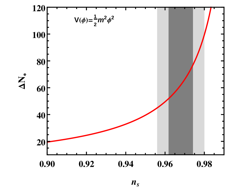
(a)

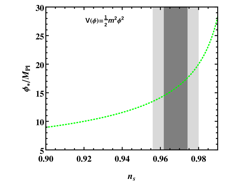
(b)

Figure 1: The variation of (a) $\Delta N_{*}$ and (b) $\frac{\phi_{*}}{M_{\text{Pl}}}$ as a function of scalar spectral index $n_{s}$ within the large field model $V(\phi)=\frac{1}{2}m^{2}\phi^{2}$. The dark gray and light gray shaded regions correspond to the 1$\sigma$ and 2$\sigma$ bounds respectively on $n_{s}$ from Planck 2015 data (TT+Low P + Lensing) [23, 24].

Further, in this model one obtains the relation

$$H_{*}=\pi M_{\text{Pl}}\sqrt{2A_{s}(1-n_{s})}.$$ (3.5)

where $n_{s}$ although strictly $k$ dependent has been replaced by it’s almost constant value. This, along with the relation of $H$ and field $\phi$ in this model, and the criterion for the end of inflation as used in (3.2), gives the value of $V$ at the end of the inflation, $V_{\text{end}}$, as a function of $A_{s}$ and $n_{s}$,

$$V_{\text{end}}=\frac{1}{2}m^{2}\phi_{\text{end}}^{2}\approx\frac{3}{2}\pi^{2}A_{s}M_{\text{Pl}}^{4}(1-n_{s})^{2}.$$ (3.6)

After substituting eq. (3.5) and (3.6) in eq. (2.23) and (2.24) we can write the temperature at the end of reheating, $T_{\text{reh}}$, and reheating e-folds, $N_{\text{reh}}$, in terms of $A_{s}$ and $n_{s}$ for the pivot scale as given below

$$\ln\left(T_{\text{reh}}\right) =\frac{3(1+\bar{w}_{\text{reh}})}{3\bar{w}_{\text{reh}}-1}\Bigg{\{}\ln\left(\pi M_{\text{Pl}}\sqrt{2A_{s}(1-n_{s})}\right)-\ln\left(\frac{k_{*}}{a_{0}}\right)-\ln\left((1+z_{\text{eq}}\right)-\left(\frac{2}{1-n_{s}}-\frac{1}{2}\right)$$ (3.7)

$$+\ln\left(\rho_{\text{eq}}^{\frac{1}{4}}\right)\Bigg{\}}-\frac{1}{3\bar{w}_{\text{reh}}-1}\ln\left(\frac{9}{4}M_{\text{Pl}}^{4}\pi^{2}A_{s}(1-n_{s})^{2}\right)-\frac{1}{4}\ln\left(\frac{\pi^{2}}{30}g_{\text{reh}}\right).$$

$$N_{\text{reh}}= \frac{1}{3\bar{w}_{\text{reh}}-1}\ln\left(\frac{9}{4}M_{\text{Pl}}^{4}\pi^{2}A_{s}(1-n_{s})^{2}\right)+\frac{4}{3\bar{w}_{\text{reh}}-1}\Bigg{\{}\ln\left(\frac{k_{*}}{a_{0}}\right)+\ln\left(1+z_{\text{eq}}\right)$$ (3.8)

$$+\left(\frac{2}{1-n_{s}}-\frac{1}{2}\right)-\ln\left(\pi M_{\text{Pl}}\sqrt{2A_{s}(1-n_{s})}\right)-\ln\left(\rho_{\text{eq}}^{\frac{1}{4}}\right)\Bigg{\}}.$$

Now, we need information about the mass scale “$m$” which can obtained by combining eqs. (3.1) and (3.5). Using Planck’s central value of $A_{s}=2.139\times 10^{-9}~{}\text{and}~{}n_{s}=0.968$ [23, 24] we obtain $m=1.38\times 10^{13}$ GeV and thus $V_{\text{end}}=(5.8\times 10^{15}\text{GeV})^{4}$. After substituting the values of $V_{\text{end}}$ and $g_{\text{reh}}\approx 100$ in eq. (2.15), one obtains the relation among $T_{\text{reh}}$, $N_{\text{reh}}$ and $\bar{w}_{\text{reh}}$ for this quadratic large field model as given below

$$N_{\text{reh}}\approx\frac{142.12}{3(1+\bar{w}_{\text{reh}})}-\frac{4}{3(1+\bar{w}_{\text{reh}})}\ln{T_{\text{reh}}}$$ (3.9)

We represent the results graphically as parametric plots of $T_{\text{reh}}$ and $N_{\text{reh}}$ in figure 2 using eq. (3.9), and figure 3 by using eq. (3.7) and eq. (3.8). The figure 2(a) represents the variation of the reheat temperature at the end of reheating, $T_{\text{reh}}$, with reheating e-folds, $N_{\text{reh}}$, for six different values of the average equation of state parameter $\bar{w}_{\text{reh}}$. In figure 2(b), the reheating e-folds $N_{\text{reh}}$ as a function of the average equation of state parameter $\bar{w}_{\text{reh}}$ is shown for six different values of $T_{\text{reh}}$. From figure 2, we see that for instantaneous reheating, $N_{\text{reh}}\rightarrow 0$, the temperature at the end of reheating is maximum and it is same for all values of $\bar{w}_{\text{reh}}$, which is the point where all curves converge in figure 2(a).

The relations of $T_{\text{reh}}$ and $N_{\text{reh}}$ to $n_{s}$, using eq. (3.7) and eq. (3.8) are shown in figure 3. Planck’s central value of $A_{s}=2.139\times 10^{-9}$ and $z_{\text{eq}}=3365$ are used and the parameter $\rho_{\text{eq}}$ is computed to be $10^{-9}$ GeV [23, 24] to obtain the figure 3. Within Planck’s 1$\sigma$ bound on $n_{s}(0.968\pm 0.006)$ [23] in figure 3(a), curves for $-\frac{1}{3}\leq\bar{w}_{\text{reh}}\leq 0$ predict $T_{\text{reh}}>10^{7}$ GeV, while the other curves ( $\frac{1}{6}\leq\bar{w}_{\text{reh}}\leq 1$) give all possible allowed values of reheat temperature ($10^{-2}$ GeV to $10^{16}$ GeV). The $1\sigma$ and $2\sigma$ bounds on $n_{s}$ yield $0.104\leq r\leq 0.152$ and $0.080\leq r\leq 0.176$ respectively for $\frac{1}{2}m^{2}\phi^{2}$ potential. From figure 3(a), the corresponding $n_{s}$ range for $\frac{1}{6}\leq\bar{w}_{\text{reh}}\leq 1$ is $0.962\lesssim n_{s}\lesssim 0.972$ which gives the upper and lower bounds on tensor to scalar ratio is $0.112\lesssim r\lesssim 0.152$. However, the upper bounds on the tensor to scalar ratio from recent observation is $r<0.09$ [23, 24]. Hence, it is very difficult to find a feasible reheating scenario for $\frac{1}{2}m^{2}\phi^{2}$ inflaton potential if the primordial gravitational waves are not detected.

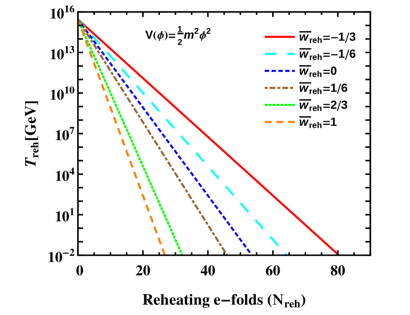
(a)

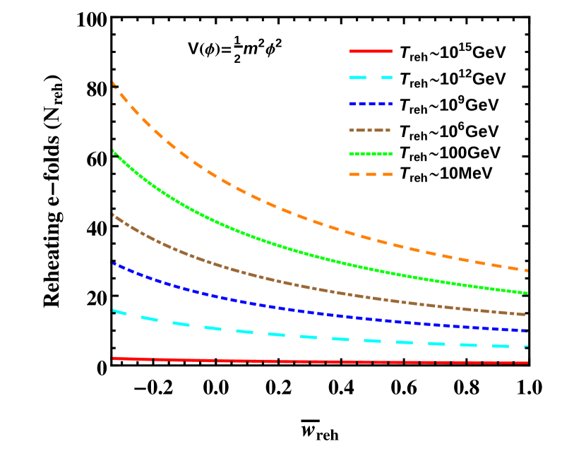
(b)

Figure 2: Plots for Large field model ($V(\phi)=\frac{1}{2}m^{2}\phi^{2}$). Plot (a) shows the variation of $T_{\text{reh}}$ with $N_{\text{reh}}$ for different values of $\bar{w}_{\text{reh}}$: $\bar{w}_{\text{reh}}=-\frac{1}{3}$ (solid red), $\bar{w}_{\text{reh}}=-\frac{1}{6}$ (large dashed cyan), $\bar{w}_{\text{reh}}=0$ (small dashed blue), $\bar{w}_{\text{reh}}=\frac{1}{6}$ (dot-dashed brown), $\bar{w}_{\text{reh}}=\frac{2}{3}$ (tiny dashed green), $\bar{w}_{\text{reh}}=1$ (medium dashed orange). Plot (b) shows $N_{\text{reh}}$ as a function of $\bar{w}_{\text{reh}}$ for different values of $T_{\text{reh}}$: $T_{\text{reh}}\sim 10^{15}\text{GeV}$ (solid red), $T_{\text{reh}}\sim 10^{12}\text{GeV}$ (large dashed cyan),$T_{\text{reh}}\sim 10^{9}\text{GeV}$ (small dashed blue), $T_{\text{reh}}\sim 10^{6}\text{GeV}$ (dot-dashed brown), $T_{\text{reh}}\sim 100\text{GeV}$ (tiny dashed green), $T_{\text{reh}}\sim 10\text{MeV}$ (medium dashed orange).

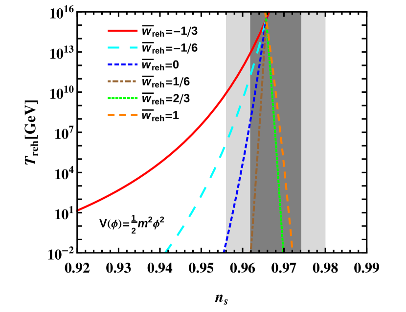
(a)

(b)

Figure 3: Plots for Large field model ($V(\phi)=\frac{1}{2}m^{2}\phi^{2}$). (a) $T_{\text{reh}}$ and (b) $N_{\text{reh}}$ as a function of $n_{s}$ for different values of $\bar{w}_{\text{reh}}$: $\bar{w}_{\text{reh}}=-\frac{1}{3}$ (solid red), $\bar{w}_{\text{reh}}=-\frac{1}{6}$ (large dashed cyan), $\bar{w}_{\text{reh}}=0$ (small dashed blue), $\bar{w}_{\text{reh}}=\frac{1}{6}$ (dot-dashed brown), $\bar{w}_{\text{reh}}=\frac{2}{3}$ (tiny dashed green), $\bar{w}_{\text{reh}}=1$ (medium dashed orange). The dark gray and light gray shaded region corresponds to the 1$\sigma$ and 2$\sigma$ bounds on $n_{s}$ from Planck 2015 data (TT+Low P + Lensing) [23, 24].

3.2 Small field /Hilltop inflation:

In this model, inflation occurs at very small value of the field and at the top of the flat potential. The potential for this kind of inflation is described by [3, 73, 7].

$$V(\phi)=V_{0}\left[1-\left(\frac{\phi}{\mu}\right)^{p}\right].$$ (3.10)

The field value at the end of inflation is calculated by setting $\epsilon=1$ and $\phi_{\text{end}}<\mu$ which leads to the following equation

$$\left(\frac{\phi_{\text{end}}}{\mu}\right)^{p}+\frac{p}{\sqrt{2}}\frac{M_{\text{Pl}}}{\mu}\left(\frac{\phi_{\text{end}}}{\mu}\right)^{p-1}=1.$$ (3.11)

As per ref. [51], we have considered $p=4$ and $\mu=15M_{\text{Pl}}$ and obtained $\frac{\phi_{\text{end}}}{M_{\text{Pl}}}=14.34$. For this quartic hilltop potential the Hubble parameter, defined in eq. (2.20), at the time of Hubble crossing of the scale $k$ takes the form

$$H_{k}^{2}=\frac{1}{M_{\text{Pl}}^{2}}\left(\frac{V_{k}}{3-\epsilon_{k}}\right)=\frac{V_{0}}{M_{\text{Pl}}^{2}}\left(\frac{1-\left(\frac{\phi_{k}}{15M_{\text{Pl}}}\right)^{4}}{3-\frac{1}{2}\left(\frac{-4\left(\frac{\phi_{k}}{M_{\text{Pl}}}\right)^{3}}{15^{4}-\left(\frac{\phi_{k}}{M_{\text{Pl}}}\right)^{4}}\right)^{2}}\right).$$ (3.12)

As in the case of the large field quadratic model, we have to write the expressions for $T_{\text{reh}}$ and $N_{\text{reh}}$ as a function of $n_{s}$ and $A_{s}$. From eq. (2.5) the expression for the number of e-folds between the horizon exit of the pivot scale and the end of inflation is given by

$$\begin{aligned} \Delta N_{*}&=\frac{1}{M_{\text{Pl}}^{2}}\int_{\phi_{\text{end}}}^{\phi_{*}}{-\frac{\mu^{p}-\phi^{p}}{p\phi^{p-1}}d\phi}\\ &=\frac{1}{M_{\text{Pl}}^{2}}\left[\frac{\mu^{p}}{p}\left(\frac{\phi_{\text{end}}^{2-p}}{2-p}-\frac{\phi_{*}^{2-p}}{2-p}\right)-\frac{1}{p}\left(\frac{\phi_{\text{end}}^{2}}{2}-\frac{\phi_{*}^{2}}{2}\right)\right].\end{aligned}$$ (3.13)

For $p=4$ and $\mu=15M_{\text{Pl}}$ the eq. (3.13) becomes

$$\Delta N_{*}=6.328\times 10^{3}\left[\left(\frac{M_{\text{Pl}}}{\phi_{*}}\right)^{2}-\left(\frac{1}{14.34}\right)^{2}\right]+\frac{1}{8}\left[\left(\frac{\phi_{*}}{M_{\text{Pl}}}\right)^{2}-(14.34)^{2}\right].$$ (3.14)

We can write the field value at the time of horizon crossing of the pivot scale as a function of $n_{s}$ as given below

$$\begin{aligned} n_{s}&=1-6\epsilon_{*}+2\eta_{*}\\ &=1-3M_{\mathrm{Pl}}^{2}\left(-\frac{4\phi_{*}^{3}}{(15M_{\mathrm{Pl}})^{4}-\phi_{*}^{4}}\right)^{2}-\frac{24\phi_{*}^{2}}{(15M_{\mathrm{Pl}})^{4}-\phi_{*}^{4}}M_{\mathrm{Pl}}^{2}\end{aligned}$$ (3.15)

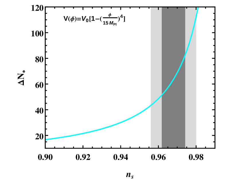
(a)

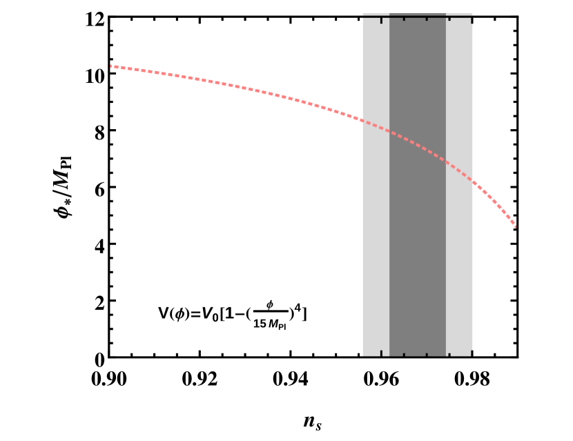
(b)

Figure 4: (a) The number of e-folds remains ($\Delta N_{*}$) after the Hubble crossing of the pivot scale ($k_{*}$) and (b) $\frac{\phi_{*}}{M_{\text{Pl}}}$ as a function of $n_{s}$ for small field/hilltop inflation with $p=4$ and $\mu=15M_{\text{Pl}}$. Shading is same as figure 1.

We can write $H_{*}$ and $V_{\text{end}}$ in terms of the scalar spectral amplitude $A_{s}$ and scalar spectral index $n_{s}$ as

$$H_{*}^{2} = A_{s}8\pi^{2}M_{\text{Pl}}^{2}\epsilon_{*}=A_{s}4\pi^{2}M_{\text{Pl}}^{4}\left[\frac{-4\phi_{*}^{3}}{(15M_{\text{Pl}}^{4})-\phi_{*}^{4}}\right]^{2},$$ (3.16)

$$H_{*} = 8\pi M_{\text{Pl}}\left(\frac{\chi^{3}(n_{s})}{15^{4}-\chi^{4}(n_{s})}\right)\sqrt{A_{s}}=8\pi M_{\text{Pl}}\beta(n_{s})\sqrt{A_{s}},$$ (3.17)

$$V_{\text{end}} = \gamma A_{s}M_{\text{Pl}}^{4}\frac{\beta^{3}(n_{s})\left(3-8\beta^{2}(n_{s})\right)}{\chi^{3}(n_{s})},$$ (3.18)

where, $\chi\tiny{(n_{s})}=\frac{\phi_{*}}{M_{\text{Pl}}}(n_{s})$ is the solution of eq. (3.15) and is shown in figure 4(b). Here we define $\beta(n_{s})=\frac{\chi^{3}(n_{s})}{15^{4}-\chi^{4}(n_{s})}$ and $\gamma=5.28\times 10^{6}$. Using above expressions for $H_{*}$ and $V_{\text{end}}$ we can write out $T_{\text{reh}}$ and $N_{\text{reh}}$ as a function of $n_{s}$ for the pivot scale but we shall not display the expressions here. Finally the parameter $V_{0}$ entering in eq. (3.10) can be determined by using eqs. (3.12) and (3.17). For hilltop potential with $p=4$ and $\mu=15M_{\text{Pl}}$ using Planck’s central value of $n_{s}=0.968$ we get $V_{0}=(1.04\times 10^{16}\text{GeV})^{4}$ and $V_{\text{end}}=(6.64\times 10^{15}\text{GeV})^{4}$ which strongly places inflation in the Grand Unification epoch. After substituting the values of $V_{\text{end}}$ and $g_{\text{reh}}\approx 100$ in eq. (2.15) we obtain the relation

$$N_{\text{reh}}\approx\frac{142.64}{3(1+\bar{w}_{\text{reh}})}-\frac{4}{3(1+\bar{w}_{\text{reh}})}\ln T_{\text{reh}}.$$ (3.19)

.

The above results are represented graphically in figure 5 and figure 6. The figure 5(a) represents the variation of $T_{\text{reh}}$ with $N_{\text{reh}}$ for different values of $\bar{w}_{\text{reh}}$ for quartic hilltop model. The length of reheating $N_{\text{reh}}$ as a function of $\bar{w}_{\text{reh}}$ is shown in figure 5(b). The variation of $T_{\text{reh}}$ and $N_{\text{reh}}$ as a function of $n_{s}$ are shown in figure 6 for different values of $\bar{w}_{\text{reh}}$. Within Planck’s 1$\sigma$ bounds on $n_{s}$, curves with $\bar{w}_{\text{reh}}<0$ ( $\bar{w}_{\text{reh}}=-\frac{1}{3}$ and $-\frac{1}{6}$ ) estimate $T_{\text{reh}}\gtrsim 10^{12}$ GeV as shown in figure 6. The curves with $\bar{w}_{\text{reh}}\geq\frac{1}{6}$ span the entire range of reheating temperature i.e., $10^{-2}$ GeV to $10^{16}$ GeV within Planck’s $1\sigma$ bounds on $n_{s}$. For this quartic hilltop model the tensor to scalar ratio r and the tensor tilt $n_{T}$ can be written as a function of $n_{s}$ and are given below

$$r=16\epsilon=128\beta^{2}(n_{s})~{}~{}~{}~{}~{}\text{and}~{}~{}~{}~{}~{}n_{T}=-16\beta^{2}(n_{s})$$ (3.20)

For the hilltop potential with $p=4$ and $\mu=15M_{\text{Pl}}$, using eq. (3.20) the $1\sigma$ and $2\sigma$ bounds on $n_{s}$ yield $0.006\leq r\leq 0.015$ and $0.003\leq r\leq 0.020$ respectively. The constraint on the tensor to scalar ratio $r\leq 0.02$ is obtained from figure 6(a) for $\bar{w}_{\text{reh}}\geq\frac{1}{6}$ and $10^{-2}$ GeV $\leq T_{\text{reh}}\leq 10^{16}$ GeV within Planck’s $1\sigma$ bounds on $n_{s}$. From figure 6(a), the upper bound $r\leq 0.015$ is estimated for $\bar{w}_{\text{reh}}\geq 0$ and $10^{-2}$ GeV $\leq T_{\text{reh}}\leq 10^{16}$ GeV within Planck’s $2\sigma$ bounds on $n_{s}$.

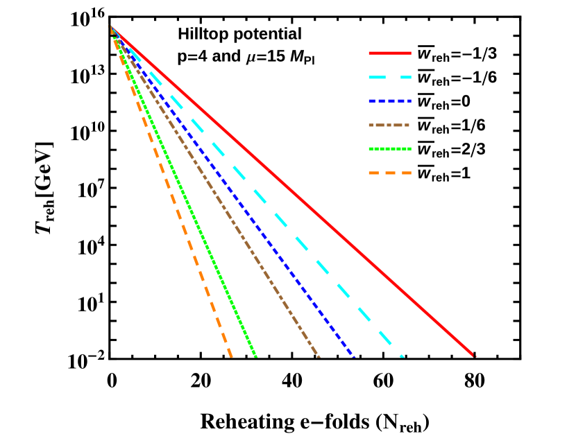
(a)

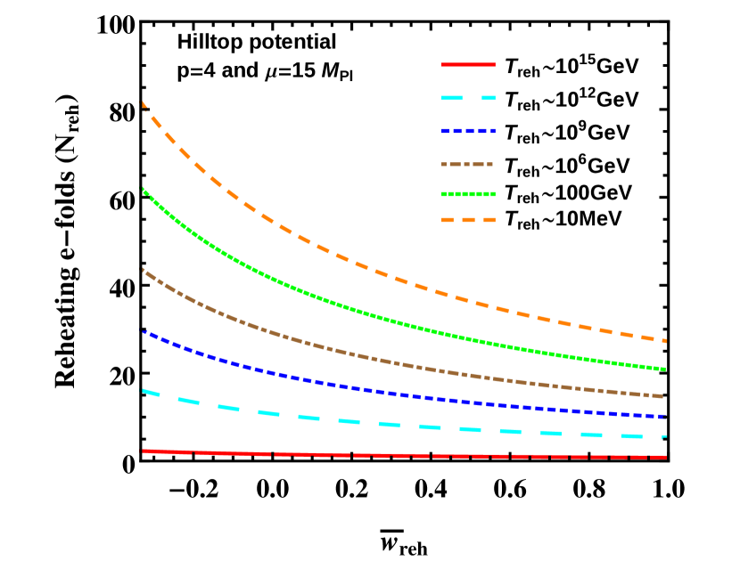
(b)

Figure 5: Plots of (a) $T_{\text{reh}}$ with $N_{\text{reh}}$ and (b) $N_{\text{reh}}$ as a function of $\bar{w}_{\text{reh}}$ for small field model with the same color coding as figure 2.

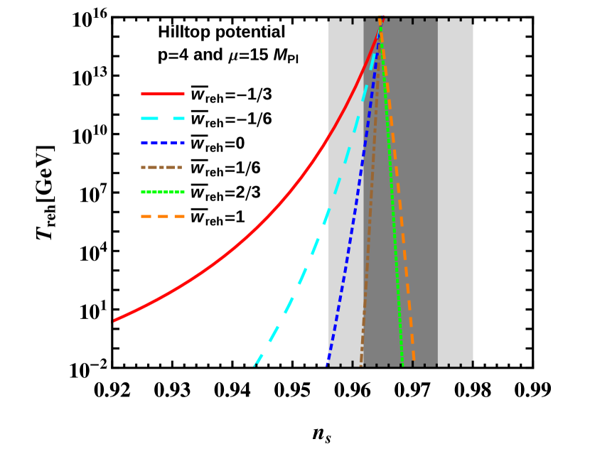
(a)

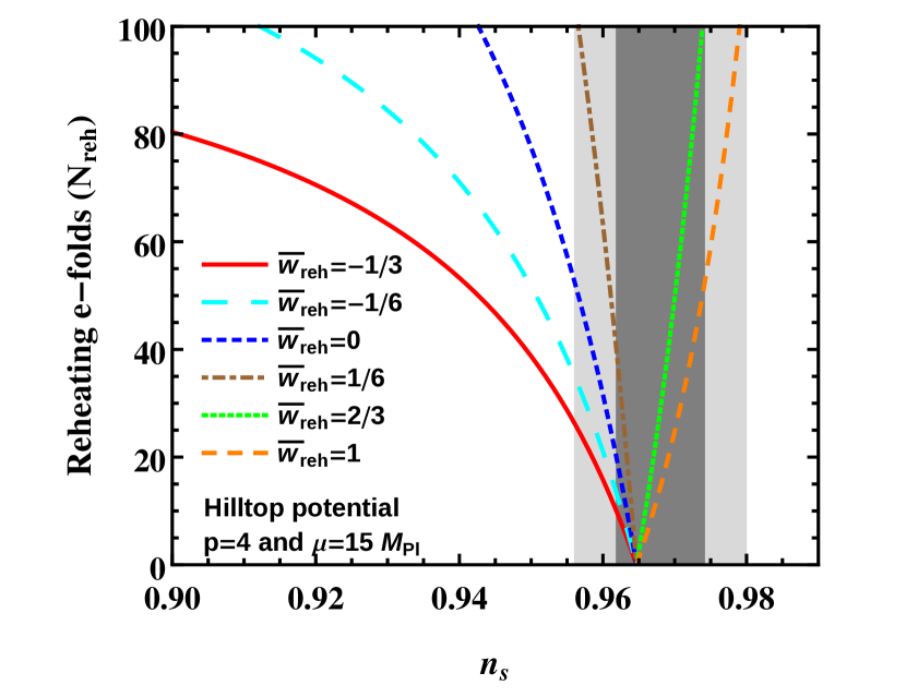
(b)

Figure 6: Plots of $T_{\text{reh}}$ and $N_{\text{reh}}$ as a function of $n_{s}$, for small field model . All curves and shaded regions are as for figure 3.

3.3 Starobinsky Model:

The action for the Starobinsky model is

$$S=\frac{1}{2}\int{d^{4}x\sqrt{-g}\left(M_{\text{Pl}}^{2}R+\frac{1}{6M^{2}}R^{2}+\mathcal{L}_{\text{matter}}\right)},$$ (3.21)

where $R$ is the Ricci scalar and $\mathcal{L}_{\text{matter}}$ is the Lagrangian for the matter content of the Universe. After performing the conformal transformation [74] to Einstein frame we get the action for the Starobinsky model which is equivalent to the scalar field version [75, 41], and is given below

$$S=\int{d^{4}x\Bigg{[}\frac{M_{\text{Pl}}^{2}}{2}R-\frac{1}{2}}\partial_{\mu}\phi\partial^{\mu}\phi-\frac{3}{4}M_{\text{Pl}}^{2}M^{2}\left(1-e^{-\sqrt{\frac{2}{3}}\phi/M_{\text{Pl}}}\right)^{2}\Bigg{]}.$$ (3.22)

Hence, in Einstein frame the Lagrangian becomes normal gravity plus a scalar field $\phi$ with the potential [75]

$$V(\phi) =\frac{3}{4}M_{\text{Pl}}^{2}M^{2}\left(1-e^{-\sqrt{\frac{2}{3}}\phi/M_{\text{Pl}}}\right)^{2}$$ (3.23)

$$=\Lambda^{4}\left(1-e^{-\sqrt{\frac{2}{3}}\phi/M_{\text{Pl}}}\right)^{2}.$$

For the above potential given in eq. (3.23), the slow-roll parameters take the form

$$\epsilon=\frac{4}{3}\frac{1}{\left(1-e^{\sqrt{\frac{2}{3}}\phi/M_{\text{Pl}}}\right)^{2}}\hskip 28.45274pt\text{and}\hskip 28.45274pt\eta=\frac{4}{3}\frac{\left(2e^{-\sqrt{\frac{2}{3}}\phi/M_{\text{Pl}}}-1\right)e^{-\sqrt{\frac{2}{3}}\phi/M_{Pl}}}{\left(1-e^{-\sqrt{\frac{2}{3}}\phi/M_{\text{Pl}}}\right)^{2}}.$$ (3.24)

The Hubble parameter as defined in eq. (2.20) at the time of Hubble crossing of the scale $k$ is given by

$$H_{k}^{2}=\frac{\Lambda^{4}}{M_{\text{Pl}}^{2}}\left(\frac{\left(1-e^{-\sqrt{\frac{2}{3}}\phi_{k}/M_{\text{ Pl }}}\right)^{2}}{3-\frac{4}{3}\left(\frac{1}{1-e^{\sqrt{\frac{2}{3}}\phi_{k}/M_{\text{Pl}}}}\right)^{2}}\right).$$ (3.25)

The number of e-folds remaining after the scale $k$ crosses the Hubble radius is obtained by using eq. (2.5), and is written below

$$\Delta N_{k}=\frac{3}{4}\left[e^{\sqrt{\frac{2}{3}}\phi_{k}/M_{Pl}}-\left(1+\frac{2}{\sqrt{3}}\right)+\ln\left(1+\frac{2}{\sqrt{3}}\right)\right]-\sqrt{\frac{3}{8}}\frac{\phi_{k}}{M_{Pl}}.$$ (3.26)

Now, similar to the large field and hilltop model we have to express $T_{\text{reh}}$ and $N_{\text{reh}}$ as a function of the experimentally estimated parameters $A_{s}$ and $n_{s}$. The scalar spectral index $n_{s}$ as defined in eq. (2.2) for this model becomes

$$n_{s}=1-\frac{8}{3}\frac{\left(1+e^{\sqrt{\frac{2}{3}}\phi_{*}/M_{\text{Pl}}}\right)}{\left(1-e^{\sqrt{\frac{2}{3}}\phi_{*}/M_{\text{Pl}}}\right)^{2}}.$$ (3.27)

From the above expression, eq. (3.27), we can write the field value at the time of Hubble crossing of the pivot scale $k_{*}$ as a function of $n_{s}$ as

$$\frac{\phi_{*}}{M_{\text{Pl}}}=\sqrt{\frac{3}{2}}\ln\left(\frac{8}{3(1-n_{s})}\right).$$ (3.28)

Now, we can write $\Delta N_{*}$, $H_{*}$ and $V_{\text{end}}$ as a function of the scalar spectral index $n_{s}$ as following

$$\Delta N_{*}=\frac{3}{4}\left[\frac{8}{3(1-n_{s})}-\left(1+\frac{2}{\sqrt{3}}\right)-\ln\left(\frac{8}{(1-n_{s})(3+2\sqrt{3})}\right)\right],$$ (3.29)

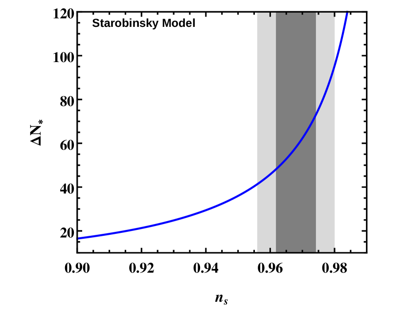
(a)

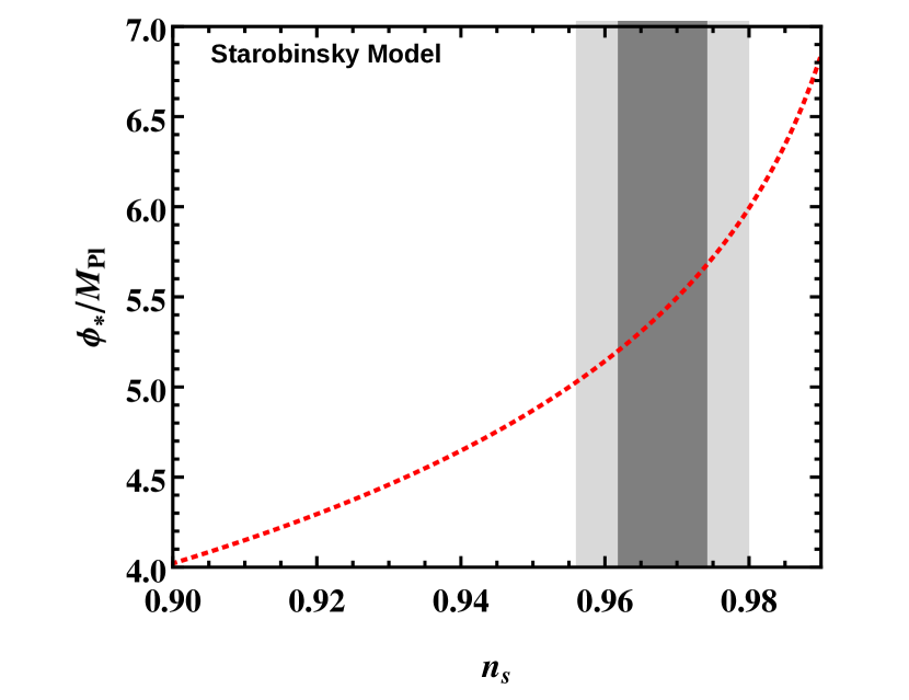
(b)

Figure 7: The variation of (a) $\Delta N_{*}$ and (b) $\frac{\phi_{*}}{M_{\text{Pl}}}$ as a function of scalar spectral index $n_{s}$ for Starobinsky model. Shading is same as figure 1

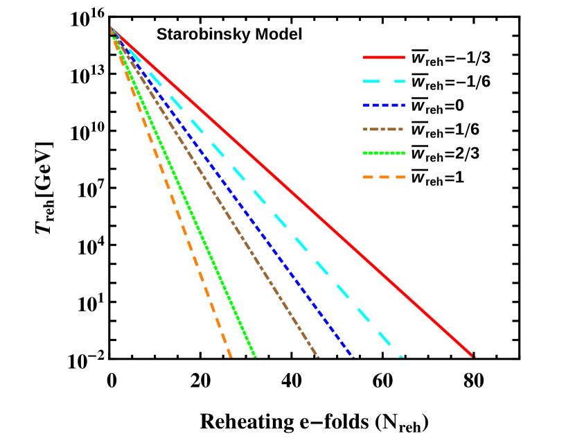
(a)

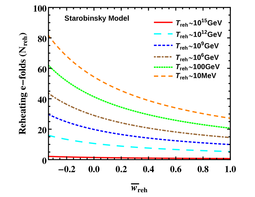
(b)

Figure 8: Plots of (a) $T_{\text{reh}}$ with $N_{\text{reh}}$ and (b) $N_{\text{reh}}$ as a function of $\bar{w}_{\text{reh}}$ for Starobinsky model with the same color coding as figure 2.

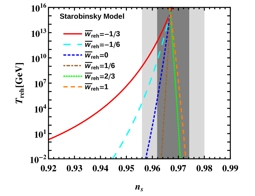
(a)

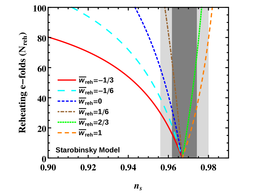
(b)

Figure 9: Plots of $T_{\text{reh}}$ and $N_{\text{reh}}$ as a function of $n_{s}$, for Starobinsky model . All curves and shaded regions are as for figure 3.

$$H_{*}\approx\pi M_{\text{Pl}}\left(1-n_{s}\right)\sqrt{\frac{3}{2}A_{s}}$$ (3.30)

and

$$V_{\text{end}}\approx\frac{9}{2}\pi^{2}A_{s}M_{\text{Pl}}^{4}(1-n_{s})^{2}\frac{1}{\left(1+\frac{\sqrt{3}}{2}\right)^{2}}.$$ (3.31)

Since $n_{s}\approx 1$, we have set $[1-x(1-n_{s})]\approx 1$ in eqs. (3.30) and (3.31) where $x$ also remains less than unity in magnitude. After substituting the above expressions for $H_{*},~{}\Delta N_{*}~{}\text{and}~{}V_{\text{end}}$ in eqs. (2.23) and (2.24) we can write the expressions of $T_{\text{reh}}$ and $N_{\text{reh}}$ as a function of $n_{s}$ for the pivot scale. The variation of $\Delta N_{*}$ and $\frac{\phi_{*}}{M_{\text{Pl}}}$ as a function of $n_{s}$ for this model are shown in figure 7 By using Planck’s central value of $A_{s}=2.139\times 10^{-9}$ and $n_{s}=0.968$ we get $\Lambda=(1.04\times 10^{16}\text{GeV})^{4}$ and $V_{\text{end}}=(6.26\times 10^{15}\text{GeV})^{4}$ for the Starobinsky model, where eqs. (3.25) and (3.30) are employed. After substituting the values of $V_{\text{end}}$ and $g_{\text{reh}}$ in (2.15), we obtain the relation

$$N_{\text{reh}}=\frac{142.42}{3(1+\bar{w}_{\text{reh}})}-\frac{4}{3(1+\bar{w}_{\text{reh}})}\ln T_{\text{reh}}~{}.$$ (3.32)

The above results are represented graphically in figure 8 and figure 9. From figure 9 we see that for $\frac{1}{6}\leq\bar{w}_{\text{reh}}\leq 1$ the entire range of reheating temperature $10^{-2}\text{GeV}\lesssim T_{\text{reh}}\lesssim 10^{16}\text{GeV}$ compatible with BBN and inflation energy scales is allowed for Planck’s $1\sigma$ limits on $n_{s}$. However, for $-\frac{1}{3}\leq\bar{w}_{\text{reh}}<\frac{1}{6}$ there is a lower bound on $T_{reh}$. For example, with $\bar{w}=-\frac{1}{3}$, $T_{\text{reh}}\gtrsim 10^{12}\text{GeV}$. For Starobinsky model the tensor to scalar ratio $r$ can be written in terms of the scalar spectral index $n_{s}$ as $r\approx 3(1-n_{s})^{2}$. These ranges of $r$ are well inside the upper bound of $r$ from recent observations [23].

4 Constraints on the reheating parameters from a step in the inflaton potential

In the previous section the expressions for $T_{\text{reh}}$ and $N_{\text{reh}}$ are written as a function of $\bar{w}_{\text{reh}}$, $n_{s}$ and $A_{s}$, see eqs. (3.7) and (3.8). However, we can also write $T_{\text{reh}}$ and $N_{\text{reh}}$ in terms of the inflaton field location $\phi_{k}$ and the number of e-folds remaining, $\Delta N_{k}$, after a given scale $k$ crosses the Hubble radius. Consider the case of the quadratic large field model in which after substituting $V_{\text{end}}=\frac{1}{2}m^{2}\phi_{\text{end}}^{2}$ and eq. (3.1) in eqs. (2.23) and (2.24) the expressions for $T_{\text{reh}}$ and $N_{\text{reh}}$ take the form

$$\ln\left(T_{\text{reh}}\right)=\frac{3(1+\bar{w}_{\text{reh}})}{3\bar{w}_{\text{reh}}-1} \Bigg{\{}\ln\left(m\sqrt{\frac{\frac{1}{2}\left(\frac{\phi_{k}}{M_{\text{Pl}}}\right)^{2}}{3-2\left(\frac{M_{\text{Pl}}}{\phi_{k}}\right)^{2}}}\right)-\ln\left(\frac{k}{a_{0}}\right)-\ln\left(1+z_{\text{eq}}\right)-\Delta N_{k}$$ (4.1)

$$+\ln\left(\rho_{\text{eq}}^{\frac{1}{4}}\right)\Bigg{\}}-\frac{1}{3\bar{w}_{\text{reh}}-1)}\ln\left(\frac{3}{4}m^{2}\phi_{\text{end}}^{2}\right)-\frac{1}{4}\ln\left(\frac{\pi^{2}}{30}g_{\text{reh}}\right).$$

$$N_{\text{reh}}=\frac{1}{3\bar{w}_{\text{reh}}-1}\ln\left(\frac{3}{4}m^{2}\phi_{\text{end}}^{2}\right)+\frac{4}{3\bar{w}_{\text{reh}}-1}\Bigg{\{} \ln\left(\frac{k}{a_{0}}\right)+\ln\left(1+z_{\text{eq}}\right)+\Delta N_{k}-\ln\left(\rho_{\text{eq}}^{\frac{1}{4}}\right)$$ (4.2)

$$-\ln\left(m\sqrt{\frac{\frac{1}{2}\left(\frac{\phi_{k}}{M_{\text{Pl}}}\right)^{2}}{3-2\left(\frac{M_{\text{Pl}}}{\phi_{k}}\right)^{2}}}\right)\Bigg{\}}$$

Similarly, we can write out the expressions of $T_{\text{reh}}$ and $N_{\text{reh}}$ for quartic hilltop and Starobinsky model but these are not displayed here. If we know the field location $\phi_{k}$ for the mode with wavenumber $k$ then the $\Delta N_{k}$ can be computed by using eq. (2.5), which leads to express $T_{\text{reh}}$ and $N_{\text{reh}}$ as a function of $\bar{w}_{\text{reh}}$ only. Using this method we proceed to strengthen our previous section’s results (i.e. the allowed ranges of $T_{\text{reh}}$, $N_{\text{reh}}$ and $\bar{w}_{\text{reh}}$) by considering an observable scale $k$ at current epoch where local anomalies have been observed in the CMB angular power spectrum.

The WMAP collaboration [17, 14, 15, 16] reported a dip and a bump near the multipoles $\ell=22$ and $\ell=40$ in the CMB angular power spectrum. The large scale power suppression, namely the dip near $\ell=22$, is also found in Planck 2013 and 2015 data [21, 22, 23, 24]. There are studies [17, 57, 58, 59, 51, 76] which relate such anomalies to a feature in the otherwise monotonic inflaton potential. Such feature is shown to generate oscillations in the primordial power spectrum, and provide better fit to the CMB data near these multipole moments. The step is introduced by multiplying the inflaton potential by a function

$$V_{\text{step}}(\phi)=\left[1+y~{}\text{tanh}\left(\frac{\phi-\phi_{k}}{\Delta\phi}\right)\right],$$ (4.3)

where $y$, $\phi_{k}$ and $\Delta\phi$ are respectively the height, location and width of the step. The scales affected by the step are those which are crossing the horizon at the time the inflaton field reaches the step location. The details of this mechanism can be found in refs. [56, 77, 17, 57, 58, 76, 59]. The locations of the step obtained in ref. [51] are $\frac{\phi_{k}}{M_{\text{Pl}}}=14.67$ for $V(\phi)=\frac{1}{2}m^{2}\phi^{2}$ model and $\frac{\phi_{k}}{M_{\text{Pl}}}=7.888$ for $V(\phi)=V_{0}\left[1-\left(\frac{\phi}{\mu}\right)^{p}\right]$ model with $p=4$ and $\mu=15M_{\text{Pl}}$. The initial condition is considered such that the pivot scale ($\frac{k_{*}}{a_{0}}=0.05\text{Mpc}^{-1}$) leaves the Hubble radius at 50 e-folds before the end of inflation. This gives us a handle on the time scale at which that particular mode left the horizon. Using eq. (2.4) we can thus determine the number of e-folds remaining after the Hubble crossing of the mode corresponding to $\ell=22$ to be $\Delta N_{k}\approx 53$. As discussed in sec. 2, $\Delta N_{k}$ receives a small correction from the brief event of getting past the step in the potential. However, this correction remains small so long as the step itself is small, i.e. $y\ll 1$. This is demonstrated for quadratic large field and quartic hilltop potential in appendix A.

For the Starobinsky model, considering $\Delta N_{k}\approx 53$ and using eq. (3.26) we obtain the field location $\frac{\phi_{k}}{M_{\text{Pl}}}\approx 5.33$. Now, using the step location, $\frac{\phi_{k}}{M_{\text{Pl}}}$, the Hubble parameter value $H_{k}$ at the time of Hubble crossing of the scale $k$ can be found to be $H_{k}=8.27\times 10^{13}$ GeV, $2.46\times 10^{13}$ GeV and $1.37\times 10^{13}$ GeV for $V(\phi)=\frac{1}{2}m^{2}\phi^{2}$ and $V_{0}\left[1-\left(\frac{\phi}{15M_{\text{Pl}}}\right)^{4}\right]$ and Starobinsky model respectively, where eqs. (3.1), (3.12) and (3.25) are employed.

In order to use this result we need to relate the values of $\ell$ of the CMB power spectrum with the wave number of the fluctuation. A comoving scale $\lambda_{co}$ is projected on the last scattering surface on an angular scale $\theta$ is given by [12]

$$\theta=\frac{\lambda_{co}}{\int{{}_{t_{ls}}^{t_{0}}\frac{dt}{a(t)}}}=\frac{\lambda_{co}}{\int_{t_{ls}}^{t_{0}}{\frac{dt}{a_{ls}[\frac{3}{2}H_{ls}(t-t_{ls})+1]^{2/3}}}},$$ (4.4)

where, $t_{ls}$ and $t_{0}$ are last scattering and present time respectively, and with $a_{ls}$ and $H_{ls}$ the scale factor and Hubble parameter at the time of last scattering. Here we have considered the Universe is matter dominated $\left(a(t)\propto t^{2/3}\right)$ from the time of last scattering till today. This in turn allows expressing the multipole moment value $\ell$ as

$$\frac{2\pi}{\ell}\approx\theta=\frac{\lambda_{\text{ph}}H_{0}}{2}\frac{\sqrt{1+z_{ls}}}{\sqrt{1+z_{ls}}-1},$$ (4.5)

where $\lambda_{\text{ph}}$ is the physical wavelength and $z_{ls}$ is the redshift of the last scattering which is defined as $1+z_{ls}=\frac{a_{0}}{a_{ls}}$. Using eq. (4.5) we can calculate the physical wavelength ($\lambda_{\text{ph}}$) and wave-number ($k_{\text{ph}}=\frac{2\pi}{\lambda_{\text{ph}}}$) corresponding to the multipole moments $\ell$. The present values of $\lambda_{\text{ph}}$ and $k_{\text{ph}}$ corresponding to $\ell=2,22$ and $40$ are shown in table 1.

Multipole moment	Physical wavelength (Mpc)	Physical wavelength ($\text{GeV}^{-1}$)	Physical wavenumber ($\text{Mpc}^{-1}$)	Physical wavenumber (GeV)
$\ell=2$	$2.69\times 10^{4}$	$4.20\times 10^{42}$	$2.34\times 10^{-4}$	$1.50\times 10^{-42}$
$\ell=22$	$2.45\times 10^{3}$	$3.82\times 10^{41}$	$2.57\times 10^{-3}$	$1.65\times 10^{-41}$
$\ell=40$	$1.35\times 10^{3}$	$2.11\times 10^{41}$	$4.68\times 10^{-3}$	$3.00\times 10^{-41}$

Table 1: Present value of the wavelengths and wavenumbers corresponding to multipole moments $\ell=2,22$ and $40$.

Using the value $\frac{k_{(\ell=22)}}{a_{0}}\sim 2.57\times 10^{-3}\text{Mpc}^{-1}$ and $\Delta N_{k}\sim 53$ for the field location $\phi_{k}$ thus allows us to obtain relations between $T_{\text{reh}}$ and $\bar{w}_{\text{reh}}$ and $N_{\text{reh}}$ and $\bar{w}_{\text{reh}}$ directly. The mass term $m$ and the energy scales $V_{0}$ and $\Lambda$ appearing in these expressions are determined by using Planck’s central value of $n_{s}=0.968$ and $A_{s}=2.139\times 10^{-9}$ [23, 24].

The resulting plots for $T_{\text{reh}}$ and $N_{\text{reh}}$ for different inflationary models are shown in figure 10. For $V(\phi)=\frac{1}{2}m^{2}\phi^{2}$, tiny dashed red curves are plotted in figure 10(a) and figure 10(b) by using eqs. (4.1) and (4.2). The solid cyan curves in figure 10(a) and figure 10(b) represent $V(\phi)=V_{0}\left[1-\left(\frac{\phi}{15M_{\text{Pl}}}\right)^{4}\right]$. Dotdashed black curves are for the Starobinsky model. From figure 10, it can be seen that in order to get the $T_{\text{reh}}$ within the reasonable range i.e., $10^{-2}$ GeV to $10^{16}$ GeV, the $\bar{w}_{\text{reh}}$ should be less than $0.2$ for all the models which are considered here. The allowed ranges of the reheating parameters for different inflationary models from Planck data and for successful explanation of the CMB low multipole anomalies are shown in table 2.

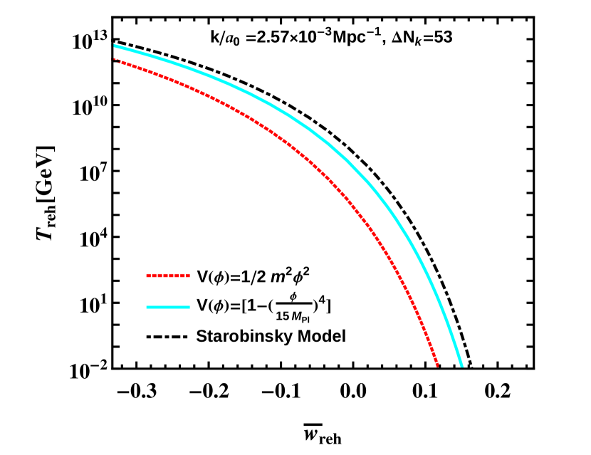
(a)

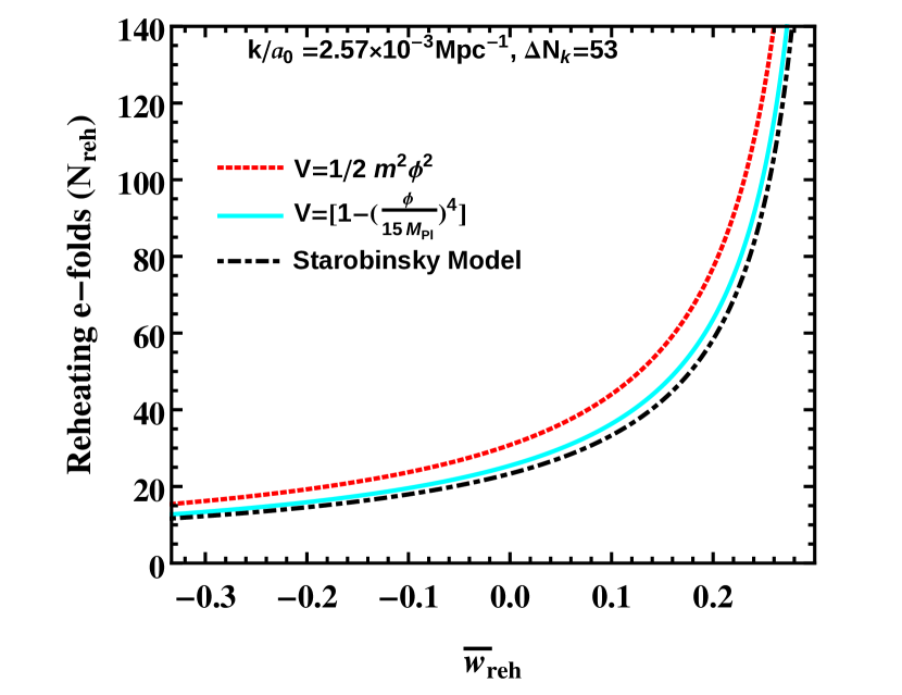
(b)

Figure 10: Plots for $T_{\text{reh}}$ and $N_{\text{reh}}$ as a function of $\bar{w}_{\text{reh}}$ for different inflationary models. Tiny dashed red curve corresponds to $V=\frac{1}{2}m^{2}\phi^{2}$ model, dotdashed black curve represents the Starobinsky model and solid cyan curve is for hilltop potential with $p=4$ and $\mu=15M_{\text{Pl}}$.

Inflationary model	Reheating parameter	Allowed range from the Planck 2015 data	Allowed range for successful explanation of CMB low multipole anomalies
Quadratic large field model	$\bar{w}_{\text{reh}}$	$-\frac{1}{3}\leq\bar{w}_{\text{reh}}\leq 1$	$-\frac{1}{3}\leq\bar{w}_{\text{reh}}\leq 0.118$
	$T_{\text{reh}}(\text{GeV})$	$10^{-2}\leq T_{\text{reh}}\leq 10^{16}$	$10^{-2}\leq T_{\text{reh}}\leq 1.21\times 10^{12}$
	$N_{\text{reh}}$	$0\leq N_{\text{reh}}\leq 74.42$	$15.41\leq N_{\text{reh}}\leq 47.65$
Hilltop model with $p=4$ and $\mu=15\text{Pl}$	$\bar{w}_{\text{reh}}$	$-\frac{1}{3}\leq\bar{w}_{\text{reh}}\leq 1$	$-\frac{1}{3}\leq\bar{w}_{\text{reh}}\leq 0.142$
	$T_{\text{reh}}(\text{GeV})$	$10^{-2}\leq T_{\text{reh}}\leq 10^{16}$	$10^{-2}\leq T_{\text{reh}}\leq 5.32\times 10^{12}$
	$N_{\text{reh}}$	$0\leq N_{\text{reh}}\leq 102.01$	$12.72\leq N_{\text{reh}}\leq 44.25$
Starobinsky model	$\bar{w}_{\text{reh}}$	$-\frac{1}{3}\leq\bar{w}_{\text{reh}}\leq 1$	$-\frac{1}{3}\leq\bar{w}_{\text{reh}}\leq 0.165$
	$T_{\text{reh}}(\text{GeV})$	$10^{-2}\leq T_{\text{reh}}\leq 10^{16}$	$10^{-2}\leq T_{\text{reh}}\leq 8.48\times 10^{12}$
	$N_{\text{reh}}$	$0\leq N_{\text{reh}}\leq 102.01$	$11.67\leq N_{\text{reh}}\leq 46.12$

Table 2: The allowed ranges of the reheating parameters from Planck data and for successful explanation of the CMB low multipole anomalies due to the features in the inflaton potential [17, 57, 58, 59, 51, 76] .

5 Discussion and Conclusions

We have traced the evolution of the observable CMB scales from the time of Hubble crossing during inflation to present time. This is done by considering an intervening epoch of reheating whose duration is parametrized by $N_{\text{reh}}$ and which is characterized by an effective equation of state parameter $\bar{w}_{\text{reh}}$. It is possible to obtain the variation of $T_{\text{reh}}$ and $N_{\text{reh}}$ as a function of the scalar spectral index $n_{s}$ for single field inflationary models and allowing a wide range of values of the average equation of state parameter $\bar{w}_{\text{reh}}$. When this is done we find that for the quadratic large field and quartic hilltop models with $\bar{w}_{\text{reh}}\in\left[{-\frac{1}{3},0}\right]$, the obtained reheat temperature range is approximately $T_{\text{reh}}\in\left[10^{6},10^{16}\right]$ GeV. If the reheat temperature is allowed to vary over the whole range $T_{\text{reh}}\in\left[10^{-2},10^{16}\right]$ GeV compatible with BBN the $\bar{w}_{\text{reh}}$ is restricted to fall within $\left[{\frac{1}{6},1}\right]$ compatible with the $1\sigma$ bounds on $n_{s}$. The same $T_{\text{reh}}$ range remains allowed to the Starobinsky model, while the range of the $\bar{w}_{\text{reh}}$ is a little wider i.e., $\bar{w}_{\text{reh}}\in\left[\approx{\frac{1}{12},1}\right]$.

However, modeling the CMB low multipole anomalies through feature in the inflaton potential gives a further handle on the reheat parameters. The obtained upper bounds on the reheating parameters for the large field, hilltop and Starobinsky model are $(\bar{w}_{\text{reh}}<0.118$, $T_{\text{reh}}<1.21\times 10^{12}\text{GeV})$, $(\bar{w}_{\text{reh}}<0.142$, $T_{\text{reh}}<5.32\times 10^{12}\text{GeV})$ and $(\bar{w}_{\text{reh}}<0.165$, $T_{\text{reh}}<8.48\times 10^{12}\text{GeV})$ respectively. However, in quadratic large field model for $\bar{w}_{\text{reh}}\leq 1$ implies $r\geq 0.112$ which is found to be greater than the recently observed upper bound on $r$ (i.e., $r<0.09$). This further strains the validity of the quadratic large field model. On the other hand, for the hilltop and Starobinsky models in the allowed $\bar{w}_{\text{reh}}$ range, the tensor to scalar ratio $r$ is always well inside the upper bounds on $r$. Hence, these models are strongly preferred for the purpose of inflationary model building. In conclusion, if the low multipole anomalies are to be successfully explained by considering a step in the inflaton potential it is possible to put stronger constraints on the reheating parameters.

Appendix A Computation of $\Delta N_{k}$ for quadratic large field and quartic hilltop potential with a step.

For the quadratic large field model the potential with the step is given by

$$V(\phi)=\frac{1}{2}m^{2}\phi^{2}\left[1+y\tanh\left(\frac{\phi-\phi_{k}}{\Delta\phi}\right)\right],$$ (A.1)

where $y,\phi_{k}~{}\text{and}~{}\Delta\phi$ are respectively the height, location and width of the step. The derivative of the potential with respect to the field $\phi$ becomes

$$V^{\prime}(\phi)=m^{2}\phi\left[1+y\tanh\left(\frac{\phi-\phi_{k}}{\Delta\phi}\right)\right]+\frac{1}{2}m^{2}\phi^{2}\frac{y}{\Delta\phi}\text{sech}^{2}\left(\frac{\phi-\phi_{k}}{\Delta\phi}\right).$$ (A.2)

The change in the potential energy due to the step, $\Delta V=2yV(\phi_{k})$, gives an additional slope

$$\frac{\Delta V}{\Delta\phi}=\frac{2yV(\phi_{k})}{\Delta\phi}.$$ (A.3)

Which should be smaller than the actual slope, i.e., $\left|\frac{\Delta V}{\Delta\phi}\right|<|V^{\prime}|$, hence

$$\left|\frac{m^{2}\phi_{k}^{2}y}{\Delta\phi}\right|<\left|m^{2}\phi_{k}\right|\Rightarrow\left|\frac{y}{\Delta\phi}\right|<\left|\frac{1}{\phi_{k}}\right|.$$ (A.4)

For the quadratic large field model with $y=16.06\times 10^{-4},~{}\phi_{k}=14.67~{}M_{\text{Pl}}~{}\text{and}~{}\Delta\phi=0.0311~{}M_{\text{Pl}}$ [51] the above condition (A.4) is satisfied. Hence we can treat the step as a small perturbation on the potential.
The equation of motion of the inflaton field is

$$\ddot{\phi}+3H\dot{\phi}+V^{\prime}(\phi)=0.$$ (A.5)

After substituting eq. (A.2) in eq. (A.5) we can write the acceleration of the inflaton field as

$$\ddot{\phi}=-3H\dot{\phi}-m^{2}\phi\left[1+y\tanh\left(\frac{\phi-\phi_{k}}{\Delta\phi}\right)\right]-\frac{1}{2}m^{2}\phi^{2}\frac{y}{\Delta\phi}\text{sech}^{2}\left(\frac{\phi-\phi_{k}}{\Delta\phi}\right).$$ (A.6)

Now, let $\dot{\phi}_{bs}$ is the velocity of the inflaton before the step. If $\dot{\phi}$ is the velocity of the field when it crossing the step at a distance $\delta\phi$ from $\phi_{bs}$ then we can write

$$\dot{\phi}^{2}-\dot{\phi}_{bs}^{2} = 2\ddot{\phi}\delta\phi$$ (A.7)

$$= -6H\dot{\phi}\delta\phi-2m^{2}\phi\left[1+y\tanh\left(\frac{\phi-\phi_{k}}{\Delta\phi}\right)\right]\delta\phi$$

$$-m^{2}\phi^{2}\frac{y\delta\phi}{\Delta\phi}\text{sech}^{2}\left(\frac{\phi-\phi_{k}}{\Delta\phi}\right).$$

However, The kinetic energy of the field can be written in terms of the slow-roll parameter even in the absence of slow roll as ( recalling eq. (2.18) which is an exact equation)

$$\frac{\dot{\phi}^{2}}{2}=\frac{\epsilon V(\phi)}{3-\epsilon}.$$ (A.8)

Thus we can approximate the change in kinetic energy as

$$\frac{1}{2}\left(\dot{\phi}^{2}-\dot{\phi}_{bs}^{2}\right)=\left(\frac{\epsilon V(\phi)}{3-\epsilon}-\frac{\epsilon_{bs}V(\phi_{bs})}{3-\epsilon_{bs}}\right)\approx\frac{\Delta\epsilon V(\phi)}{3-\epsilon}.$$ (A.9)

where we ignore corrections proportional to the parameter $y$, Substituting eq. (A.9) in eq. (A.7) we obtain

$$\frac{2\Delta\epsilon V(\phi)}{3-\epsilon} = -6H\dot{\phi}\delta\phi-2m^{2}\phi\left[1+y\tanh\left(\frac{\phi-\phi_{k}}{\Delta\phi}\right)\right]\delta\phi$$ (A.10)

$$-m^{2}\phi^{2}\frac{y\delta\phi}{\Delta\phi}\text{sech}^{2}\left(\frac{\phi-\phi_{k}}{\Delta\phi}\right).$$

Which gives

$$\dot{\phi} = -\frac{1}{3H\delta\phi}\Bigg{\{}\frac{\Delta\epsilon V(\phi)}{3-\epsilon}+m^{2}\phi\left[1+y\tanh\left(\frac{\phi-\phi_{k}}{\Delta\phi}\right)\right]\delta\phi$$ (A.11)

$$+\frac{1}{2}m^{2}\phi^{2}\frac{y\delta\phi}{\Delta\phi}\text{sech}^{2}\left(\frac{\phi-\phi_{k}}{\Delta\phi}\right)\Bigg{\}}.$$

The number of e-folds remaining after the field reaches the position $\phi_{k}$ is

$$\Delta N_{k} = \int_{\phi_{k}}^{\phi_{e}}\frac{H}{\dot{\phi}}d\phi=\int_{\phi_{k}}^{\phi_{k}-\Delta\phi}\frac{H}{\dot{\phi}}d\phi+\int_{\phi_{k}-\Delta\phi}^{\phi_{e}}\frac{H}{\dot{\phi}}d\phi$$ (A.12)

$$\approx \frac{1}{M_{\text{Pl}}^{2}}\int_{\phi_{e}}^{\phi_{k}-\Delta\phi}\frac{V}{V^{\prime}}d\phi+\int_{\phi_{k}-\Delta\phi}^{\phi_{k}}\left(-\frac{H}{\dot{\phi}}\right)d\phi$$

$$= \Delta N_{\text{SR}}+\Delta N_{\text{step}}.$$

Here the subscript ‘SR’ denotes evaluation of the quantity by considering the slow-roll approximation. For this quadratic large field potential, $\phi_{e}=\sqrt{2}M_{\text{Pl}},\phi_{k}=14.67M_{\text{Pl}}~{}\text{and}~{}\Delta\phi=0.0311M_{\text{Pl}}$ [51]. As a result we obtain

$$\Delta N_{\text{SR}}\approx\int_{\sqrt{2}}^{14.67-0.0311}\frac{V}{V^{\prime}}d\phi\approx 53.07~{}.$$ (A.13)

Now we compute $\Delta N_{\text{step}}$ as presented below

$$\Delta N_{\text{step}}=\int_{\phi_{k}-\Delta\phi}^{\phi_{k}}\left(-\frac{H}{\dot{\phi}}\right)d\phi.$$ (A.14)

After substituting the expression of $\dot{\phi}$, eq. (A.11) in eq. (A.14)

$$\Delta N_{\text{step}}=\int_{\phi_{k}-\Delta\phi}^{\phi_{k}}{\frac{3H^{2}\delta\phi}{\frac{\Delta\epsilon V(\phi)}{3-\epsilon}+m^{2}\phi\left[1+y\tanh\left(\frac{\phi-\phi_{k}}{\Delta\phi}\right)\right]\delta\phi+\frac{1}{2}m^{2}\phi^{2}\frac{y\delta\phi}{\Delta\phi}\text{sech}^{2}\left(\frac{\phi-\phi_{k}}{\Delta\phi}\right)}}d\phi.$$

$$\approx\frac{3H_{k}^{2}\Delta\phi^{2}}{\frac{\Delta\epsilon V(\phi_{k})}{3-\epsilon_{k}}+m^{2}\phi_{k}\Delta\phi+\frac{1}{2}m^{2}\phi_{k}^{2}y}$$ (A.16)

where we have estimated the integration over this short interval by the value of the integrand at $\phi_{k}$ times the width of the interval. The numerical value of $\Delta N_{\text{step}}$ is obtained by substituting the values of $\epsilon_{k}\approx 10^{-4},~{}\Delta\epsilon\approx 10^{-4},~{}y=16.06\times 10^{-4},~{}\phi_{k}=14.67~{}M_{\text{Pl}}~{}\text{and}~{}\Delta\phi_{k}=0.0031~{}M_{\text{Pl}}$ [51] and, is given by

$$\Delta N_{\text{step}}\approx 0.16~{}.$$ (A.17)

Finally, for the large field model we obtain

$$\Delta N_{k}=\Delta N_{\text{SR}}+\Delta N_{\text{step}}\approx 53.07+0.16=53.23~{}.$$ (A.18)

Now, in the case of quartic hilltop model the field is rolling from lower value to it’s higher value in the potential, hence we can write

$$\Delta N_{k} = \int_{\phi_{k}}^{\phi_{e}}\frac{H}{\dot{\phi}}d\phi=\int_{\phi_{k}}^{\phi_{k}+\Delta\phi}\frac{H}{\dot{\phi}}d\phi+\int_{\phi_{k}+\Delta\phi}^{\phi_{e}}\frac{H}{\dot{\phi}}d\phi$$ (A.19)

$$\approx \frac{1}{M_{\text{Pl}}^{2}}\int_{\phi_{e}}^{\phi_{k}+\Delta\phi}\frac{V}{V^{\prime}}d\phi+\int_{\phi_{k}+\Delta\phi}^{\phi_{k}}\left(-\frac{H}{\dot{\phi}}\right)d\phi$$

$$= \Delta N_{\text{SR}}+\Delta N_{\text{step}}.$$

For this quartic hilltop model we have $\phi_{e}=14.34M_{\text{Pl}}$, $\phi_{k}=7.888$ and $\Delta\phi=0.0090M_{\text{Pl}}$ which gives

$$\Delta N_{\text{SR}}\approx\int_{14.34}^{7.888+0.0090}\frac{V}{V^{\prime}}d\phi\approx 52.79~{}.$$ (A.20)

Now, Similar to the large field model we can write the expression of $\Delta N_{\text{step}}$ for this hilltop model, and is

$$\Delta N_{\text{step}}=\int_{\phi_{k}+\Delta\phi}^{\phi_{k}}\frac{3H^{2}\delta\phi}{\frac{\Delta\epsilon V(\phi)}{3-\epsilon}+\frac{V_{0}\phi^{3}\delta\phi}{\mu^{4}}\left[1+y\tanh\left(\frac{\phi-\phi_{k}}{\Delta\phi}\right)\right]-V_{0}\left[1-\left(\frac{\phi}{\mu}\right)^{4}\right]\frac{y\delta\phi}{\Delta\phi}\text{ sech}^{2}\left(\frac{\phi-\phi_{k}}{\Delta\phi}\right)}d\phi$$

$$\approx\frac{3H_{k}^{2}{\Delta\phi}^{2}}{\frac{\Delta\epsilon V(\phi_{k})}{3-\epsilon_{k}}+\frac{V_{0}\phi_{k}^{3}\Delta\phi}{\mu^{4}}-V_{0}y\left[1-\left(\frac{\phi_{k}}{\mu}\right)^{4}\right]}~{}.$$ (A.22)

Substituting $\epsilon_{k}\approx 10^{-4},\Delta\epsilon\approx 10^{-4},\phi_{k}=7.888M_{\text{Pl}},\Delta\phi=0.0090M_{\text{Pl}}$ and $y=-0.1569\times 10^{-3}$ [51] in eq. (A.22) we obtain

$$\Delta N_{\text{step}}\approx 0.28~{}.$$ (A.23)

Adding eqs. (A.20) and (A.23) we get

$$\Delta N_{k}=\Delta N_{\text{SR}}+\Delta N_{\text{step}}\approx 52.79+0.28=53.07~{}.$$ (A.24)

Hence from the above results, i.e., (A.18) and (A.24) we can consider that $\Delta N_{k}\approx 53$.

References

- [1] A. A. Starobinsky, A New Type of Isotropic Cosmological Models Without Singularity, Phys. Lett. 91B (1980) 99.
- [2] A. H. Guth, The Inflationary Universe: A Possible Solution to the Horizon and Flatness Problems, Phys. Rev. D23 (1981) 347.
- [3] A. D. Linde, A New Inflationary Universe Scenario: A Possible Solution of the Horizon, Flatness, Homogeneity, Isotropy and Primordial Monopole Problems, Phys. Lett. B108 (1982) 389.
- [4] S. W. Hawking, The Development of Irregularities in a Single Bubble Inflationary Universe, Phys. Lett. 115B (1982) 295.
- [5] A. D. Linde, Chaotic Inflation, Phys. Lett. B129 (1983) 177.
- [6] A. D. Linde, Inflationary Cosmology, Lect. Notes Phys. 738 (2008) 1 [0705.0164].
- [7] J. Martin, C. Ringeval and V. Vennin, Encyclopædia Inflationaris, Phys. Dark Univ. 5-6 (2014) 75 [1303.3787].
- [8] A. H. Guth and S. Y. Pi, Fluctuations in the New Inflationary Universe, Phys. Rev. Lett. 49 (1982) 1110.
- [9] A. A. Starobinsky, Dynamics of Phase Transition in the New Inflationary Universe Scenario and Generation of Perturbations, Phys. Lett. B117 (1982) 175.
- [10] V. F. Mukhanov, H. A. Feldman and R. H. Brandenberger, Theory of cosmological perturbations. Part 1. Classical perturbations. Part 2. Quantum theory of perturbations. Part 3. Extensions, Phys. Rept. 215 (1992) 203.
- [11] J. M. Bardeen, P. J. Steinhardt and M. S. Turner, Spontaneous Creation of Almost Scale - Free Density Perturbations in an Inflationary Universe, Phys. Rev. D28 (1983) 679.
- [12] A. Riotto, Inflation and the theory of cosmological perturbations, in Astroparticle physics and cosmology. Proceedings: Summer School, Trieste, Italy, Jun 17-Jul 5 2002, pp. 317–413, 2002, hep-ph/0210162.
- [13] WMAP collaboration, J. Dunkley et al., Five-Year Wilkinson Microwave Anisotropy Probe (WMAP) Observations: Likelihoods and Parameters from the WMAP data, Astrophys. J. Suppl. 180 (2009) 306 [0803.0586].
- [14] WMAP collaboration, E. Komatsu et al., Five-Year Wilkinson Microwave Anisotropy Probe (WMAP) Observations: Cosmological Interpretation, Astrophys. J. Suppl. 180 (2009) 330 [0803.0547].
- [15] E. Komatsu, K. M. Smith, J. Dunkley, C. L. Bennett, B. Gold, G. Hinshaw et al., Seven-year wilkinson microwave anisotropy probe (wmap) observations: Cosmological interpretation, The Astrophysical Journal Supplement Series 192 (2011) 18.
- [16] G. Hinshaw, D. Larson, E. Komatsu, D. N. Spergel, C. L. Bennett, J. Dunkley et al., Nine-year wilkinson microwave anisotropy probe (wmap) observations: Cosmological parameter results, The Astrophysical Journal Supplement Series 208 (2013) 19.
- [17] WMAP collaboration, H. V. Peiris et al., First year Wilkinson Microwave Anisotropy Probe (WMAP) observations: Implications for inflation, Astrophys. J. Suppl. 148 (2003) 213 [astro-ph/0302225].
- [18] D. Larson, J. Dunkley, G. Hinshaw, E. Komatsu, M. R. Nolta, C. L. Bennett et al., Seven-year wilkinson microwave anisotropy probe (wmap) observations: Power spectra and wmap-derived parameters, The Astrophysical Journal Supplement Series 192 (2011) 16.
- [19] M. L. Brown, P. Ade, J. Bock, M. Bowden, G. Cahill, P. G. Castro et al., Improved measurements of the temperature and polarization of the cosmic microwave background from quad, The Astrophysical Journal 705 (2009) 978.
- [20] C. L. Reichardt et al., High resolution CMB power spectrum from the complete ACBAR data set, Astrophys. J. 694 (2009) 1200 [0801.1491].
- [21] Planck collaboration, P. A. R. Ade et al., Planck 2013 results. XVI. Cosmological parameters, Astron. Astrophys. 571 (2014) A16 [1303.5076].
- [22] Planck collaboration, P. A. R. Ade et al., Planck 2013 results. XXII. Constraints on inflation, Astron. Astrophys. 571 (2014) A22 [1303.5082].
- [23] Planck collaboration, P. A. R. Ade et al., Planck 2015 results. XIII. Cosmological parameters, Astron. Astrophys. 594 (2016) A13 [1502.01589].
- [24] Planck collaboration, P. A. R. Ade et al., Planck 2015 results. XX. Constraints on inflation, Astron. Astrophys. 594 (2016) A20 [1502.02114].
- [25] M. S. Turner, Coherent Scalar Field Oscillations in an Expanding Universe, Phys. Rev. D28 (1983) 1243.
- [26] J. H. Traschen and R. H. Brandenberger, Particle Production During Out-of-equilibrium Phase Transitions, Phys. Rev. D42 (1990) 2491.
- [27] A. Albrecht, P. J. Steinhardt, M. S. Turner and F. Wilczek, Reheating an Inflationary Universe, Phys. Rev. Lett. 48 (1982) 1437.
- [28] L. Kofman, A. D. Linde and A. A. Starobinsky, Reheating after inflation, Phys. Rev. Lett. 73 (1994) 3195 [hep-th/9405187].
- [29] L. Kofman, A. D. Linde and A. A. Starobinsky, Towards the theory of reheating after inflation, Phys. Rev. D56 (1997) 3258 [hep-ph/9704452].
- [30] M. Drewes and J. U. Kang, The Kinematics of Cosmic Reheating, Nucl. Phys. B875 (2013) 315 [1305.0267].
- [31] R. Allahverdi, R. Brandenberger, F.-Y. Cyr-Racine and A. Mazumdar, Reheating in Inflationary Cosmology: Theory and Applications, Ann. Rev. Nucl. Part. Sci. 60 (2010) 27 [1001.2600].
- [32] J. Martin, C. Ringeval and V. Vennin, Observing Inflationary Reheating, Phys. Rev. Lett. 114 (2015) 081303 [1410.7958].
- [33] J. B. Munoz and M. Kamionkowski, Equation-of-State Parameter for Reheating, Phys. Rev. D91 (2015) 043521 [1412.0656].
- [34] G. Steigman, Primordial Nucleosynthesis in the Precision Cosmology Era, Ann. Rev. Nucl. Part. Sci. 57 (2007) 463 [0712.1100].
- [35] A. R. Liddle and S. M. Leach, How long before the end of inflation were observable perturbations produced?, Phys. Rev. D68 (2003) 103503 [astro-ph/0305263].
- [36] J. Martin and C. Ringeval, First CMB Constraints on the Inflationary Reheating Temperature, Phys. Rev. D82 (2010) 023511 [1004.5525].
- [37] L. Dai, M. Kamionkowski and J. Wang, Reheating constraints to inflationary models, Phys. Rev. Lett. 113 (2014) 041302 [1404.6704].
- [38] J. Martin and C. Ringeval, Inflation after WMAP3: Confronting the Slow-Roll and Exact Power Spectra to CMB Data, JCAP 0608 (2006) 009 [astro-ph/0605367].
- [39] P. Adshead, R. Easther, J. Pritchard and A. Loeb, Inflation and the Scale Dependent Spectral Index: Prospects and Strategies, JCAP 1102 (2011) 021 [1007.3748].
- [40] J. Mielczarek, Reheating temperature from the CMB, Phys. Rev. D83 (2011) 023502 [1009.2359].
- [41] J. L. Cook, E. Dimastrogiovanni, D. A. Easson and L. M. Krauss, Reheating predictions in single field inflation, JCAP 1504 (2015) 047 [1502.04673].
- [42] S. Hannestad, Reconstructing the inflationary power spectrum from CMBR data, Phys. Rev. D63 (2001) 043009 [astro-ph/0009296].
- [43] S. L. Bridle, A. M. Lewis, J. Weller and G. Efstathiou, Reconstructing the primordial power spectrum, Mon. Not. Roy. Astron. Soc. 342 (2003) L72 [astro-ph/0302306].
- [44] P. Mukherjee and Y. Wang, Model-independent reconstruction of the primordial power spectrum from WMAP data, Astrophys. J. 599 (2003) 1 [astro-ph/0303211].
- [45] S. Hannestad, Reconstructing the primordial power spectrum - A New algorithm, JCAP 0404 (2004) 002 [astro-ph/0311491].
- [46] A. Shafieloo and T. Souradeep, Primordial power spectrum from WMAP, Phys. Rev. D70 (2004) 043523 [astro-ph/0312174].
- [47] A. Shafieloo, T. Souradeep, P. Manimaran, P. K. Panigrahi and R. Rangarajan, Features in the Primordial Spectrum from WMAP: A Wavelet Analysis, Phys. Rev. D75 (2007) 123502 [astro-ph/0611352].
- [48] A. Shafieloo and T. Souradeep, Estimation of Primordial Spectrum with post-WMAP 3 year data, Phys. Rev. D78 (2008) 023511 [0709.1944].
- [49] R. Nagata and J. Yokoyama, Band-power reconstruction of the primordial fluctuation spectrum by the maximum likelihood reconstruction method, Phys. Rev. D79 (2009) 043010 [0812.4585].
- [50] G. Nicholson and C. R. Contaldi, Reconstruction of the primordial power spectrum using temperature and polarisation data from multiple experiments, Journal of Cosmology and Astroparticle Physics 2009 (2009) 011.
- [51] D. K. Hazra, M. Aich, R. K. Jain, L. Sriramkumar and T. Souradeep, Primordial features due to a step in the inflaton potential, JCAP 1010 (2010) 008 [1005.2175].
- [52] D. K. Hazra, A. Shafieloo, G. F. Smoot and A. A. Starobinsky, Primordial features and Planck polarization, JCAP 1609 (2016) 009 [1605.02106].
- [53] D. K. Hazra, D. Paoletti, M. Ballardini, F. Finelli, A. Shafieloo, G. F. Smoot et al., Probing features in inflaton potential and reionization history with future CMB space observations, 1710.01205.
- [54] A. A. Starobinsky, Spectrum of adiabatic perturbations in the universe when there are singularities in the inflation potential, JETP Lett. 55 (1992) 489.
- [55] C. Dvorkin and W. Hu, Generalized Slow Roll for Large Power Spectrum Features, Phys. Rev. D81 (2010) 023518 [0910.2237].
- [56] J. A. Adams, B. Cresswell and R. Easther, Inflationary perturbations from a potential with a step, Phys. Rev. D64 (2001) 123514 [astro-ph/0102236].
- [57] L. Covi, J. Hamann, A. Melchiorri, A. Slosar and I. Sorbera, Inflation and WMAP three year data: Features have a Future!, Phys. Rev. D74 (2006) 083509 [astro-ph/0606452].
- [58] J. Hamann, L. Covi, A. Melchiorri and A. Slosar, New Constraints on Oscillations in the Primordial Spectrum of Inflationary Perturbations, Phys. Rev. D76 (2007) 023503 [astro-ph/0701380].
- [59] M. J. Mortonson, C. Dvorkin, H. V. Peiris and W. Hu, CMB polarization features from inflation versus reionization, Phys. Rev. D79 (2009) 103519 [0903.4920].
- [60] M. Joy, V. Sahni and A. A. Starobinsky, A New Universal Local Feature in the Inflationary Perturbation Spectrum, Phys. Rev. D77 (2008) 023514 [0711.1585].
- [61] R. K. Jain, P. Chingangbam, J.-O. Gong, L. Sriramkumar and T. Souradeep, Punctuated inflation and the low CMB multipoles, JCAP 0901 (2009) 009 [0809.3915].
- [62] R. K. Jain, P. Chingangbam, L. Sriramkumar and T. Souradeep, The tensor-to-scalar ratio in punctuated inflation, Phys. Rev. D82 (2010) 023509 [0904.2518].
- [63] A. R. Liddle and D. H. Lyth, The Cold dark matter density perturbation, Phys. Rept. 231 (1993) 1 [astro-ph/9303019].
- [64] B. A. Bassett, S. Tsujikawa and D. Wands, Inflation dynamics and reheating, Rev. Mod. Phys. 78 (2006) 537 [astro-ph/0507632].
- [65] P. Adshead, C. Dvorkin, W. Hu and E. A. Lim, Non-Gaussianity from Step Features in the Inflationary Potential, Phys. Rev. D85 (2012) 023531 [1110.3050].
- [66] D. Boyanovsky, H. J. de Vega, R. Holman and J. F. J. Salgado, Preheating and reheating in inflationary cosmology: A Pedagogical survey, in String theory in curved space times. Proceedings, String Gravity Meeting, Paris, France, June 6-7, 1996, pp. 260–280, 1996, astro-ph/9609007.
- [67] L. Kofman, Reheating and preheating after inflation, in Particle cosmology. Proceedings, 3rd RESCEU International Symposium, Tokyo, Japan, November 10-13, 1997, pp. 1–8, 1997, hep-ph/9802285.
- [68] G. N. Felder, L. Kofman and A. D. Linde, Instant preheating, Phys. Rev. D59 (1999) 123523 [hep-ph/9812289].
- [69] G. F. Giudice, A. Riotto and I. I. Tkachev, The Cosmological moduli problem and preheating, JHEP 06 (2001) 020 [hep-ph/0103248].
- [70] M. Desroche, G. N. Felder, J. M. Kratochvil and A. D. Linde, Preheating in new inflation, Phys. Rev. D71 (2005) 103516 [hep-th/0501080].
- [71] J. Martin, Inflation and precision cosmology, Braz. J. Phys. 34 (2004) 1307 [astro-ph/0312492].
- [72] A. D. Linde, CHAOTIC INFLATING UNIVERSE, JETP Lett. 38 (1983) 176.
- [73] W. H. Kinney and K. T. Mahanthappa, Inflation from symmetry breaking below the Planck scale, Phys. Lett. B383 (1996) 24 [hep-ph/9511460].
- [74] S. Kalara, N. Kaloper and K. A. Olive, Theories of Inflation and Conformal Transformations, Nucl. Phys. B341 (1990) 252.
- [75] A. Kehagias, A. Moradinezhad Dizgah and A. Riotto, Remarks on the Starobinsky model of inflation and its descendants, Phys. Rev. D89 (2014) 043527 [1312.1155].
- [76] M. Benetti, S. Pandolfi, M. Lattanzi, M. Martinelli and A. Melchiorri, Featuring the primordial power spectrum: new constraints on interrupted slow-roll from CMB and LRG data, Phys. Rev. D87 (2013) 023519 [1210.3562].
- [77] S. M. Leach and A. R. Liddle, Inflationary perturbations near horizon crossing, Phys. Rev. D63 (2001) 043508 [astro-ph/0010082].