Surface term, corner term, and action growth in $F($Riemann$)$ gravity theory

Abstract

After reformulating $F($Riemann$)$ gravity theory as a second derivative theory by introducing two auxiliary fields to the bulk action, we derive the surface term as well as the corner term supplemented to the bulk action for a generic non-smooth boundary such that the variational principle is well posed. We also introduce the counter term to make the boundary term invariant under the reparametrization for the null segment. Then as a demonstration of the power of our formalism, not only do we apply our expression for the full action to evaluate the corresponding action growth rate of the Wheeler-DeWitt patch in the Schwarzchild anti-de Sitter black hole for the $F(R)$ gravity and critical gravity, where the corresponding late time behavior recovers the previous one derived by other approaches, but also in the asymptotically Anti-de Sitter black hole for the critical Einsteinian cubic gravity, where the late time growth rate vanishes but still saturates the Lloyd bound.

I Introduction

Generically, in order to make the variational principle well posed for gravity theories, one is required to add the surface term to the bulk action. In this way, the Gibbons-Hawking-York (GHY) surface term is introduced for the case of Einstein gravity, but is applicable only to a non-null boundaryGowdy ; York ; GH . For a null boundary, the surface term has also been investigated recentlyNeiman ; PCMP ; PCP ; LMPS ; HF . Moreover, if the boundary is non-smooth, $i.e.$, the boundary contains some corners intersected by the segments, the additional corner term has to be added to the actionHayward ; JSSS . On the other hand, although the non-null surface terms have been developed for other gravitational theories, such as $F(R)$ gravityCDM ; GCT , Gauss-Bonnet gravityBunch ; Myers , Lanczos-Lovelock theoryPK ; BCLR ; CPP ; Cano , and other higher derivative theoriesST ; TTEM ; BCR , the corresponding null surface term has not been fully explored.

However, for a generic higher order gravitational theory as usually formulated, due to higher-derivative terms, it is hard to find an appropriate surface term to make the variational principle well posedDKH . But at least for $F($Riemann$)$ gravity, this problem can be circumvented by introducing two auxiliary fields, because this allows us to recast the action as a second order gravitational theory, which is on-shell equivalent to the original actionDMY . Furthermore, if the auxiliary fields on the boundary can be shown by the Hamiltonian analysis to be independent of the extrinsic curvature, then for a smooth non-null boundary a generalized GHY term can be found to establish the well posed variational principle. In this paper, we shall focus exclusively on this situation and formulate the well posed variational principle for more general circumstances, where the boundary is not necessarily required to be non-null or smooth.

Another motivation to evaluate the full action with a non-smooth boundary including null segments comes from the “complexity equals action” (CA) conjectureBRSSZ1 ; BRSSZ2 . This conjecture states that the complexity of a particular state $|\psi(t_{L},t_{R})\rangle$ on the boundary is given by

$$\mathcal{C}\left(|\psi(t_{L},t_{R})\rangle\right)\equiv\frac{I}{\pi\hbar}\,,$$ (1)

where $I$ is the on-shell action in the corresponding Wheeler-DeWitt (WDW) patch, enclosed by the past and future light sheets sent into the bulk spacetime from the boundary time slices $t_{L}$ and $t_{R}$. As an application of our formulation of the full action for $F($Riemann$)$ gravity, we shall evaluate the action growth rate of the WDW patch in the Schwarzschild anti-de Sitter (SAdS) black hole for both the $F(R)$ gravity and critical gravity. This thus makes up the deficiency of the approaches developed in BRSSZ1 ; BRSSZ2 , which can only give rise to the late time behavior of the action growth rateAFNV ; GWLL . To further demonstrate the power of our formalism, we also evaluate the action growth rate of the WDW patch in the asymptotically AdS black hole for the critical Einsteinian cubic gravity. The resulting late time growth rate still saturates the Lloyd bound although vanishes.

This paper is structured as follows. In Sec.II, we follow the strategy developed in DMY to introduce the two auxiliary fields to reformulate the original action and evaluate its variation. After this, we derive the required boundary term to make the variational principle well posed for both non-null segments and null segments of a non-smooth boundary in Sec.III and Sec.IV, respectively. As an application of the resulting full action, Section V devotes an explicit calculation of the action growth rate for the WDW patch in the SAdS black hole for both $F(R)$ gravity and critical gravity, as well as in the asymptotically AdS black hole for the critical Einsteinian cubic gravity. We conclude our paper in Sec. VI.

II Reformulation of $F($Riemann$)$ gravity theory

The conventional bulk action for $F($Riemann$)$ gravity is given by

$$I_{\text{bulk}}=\int_{\mathcal{M}}d^{d+2}x\sqrt{-g}F(R_{abcd},g_{ab})\,$$ (2)

with $F$ an arbitrary function of $R_{abcd}$ and $g_{ab}$. Its variation can be obtained as

$$\delta I_{\text{bulk}}=\int_{\mathcal{M}}d^{d+2}x\sqrt{-g}E_{ab}\delta g^{ab}+\int_{\partial\mathcal{M}}{\mathchar 22\relax\mkern-10.0mu\delta}v^{a}d\Sigma_{a}\,.$$ (3)

Here $d\Sigma_{a}$ is the outward-directed surface element on $\partial\mathcal{M}$, and

$${\mathchar 22\relax\mkern-10.0mu\delta}v^{c} = 2P_{a}{}^{bcd}\delta{\Gamma^{a}}_{bd}+2\delta g_{bd}\nabla_{a}P^{abcd}\,$$ (4)

with $P^{abcd}=\frac{\partial F}{\partial R_{abcd}}$. In addition, the symbol ${\mathchar 22\relax\mkern-10.0mu\delta}$ indicates an infinitesimal quantity which can not be written as the variation of any quantity. Obviously, $E_{ab}=0$ is simply the equation of motion. But in order to give rise to a well posed variational principle, we must supplement a boundary term $I_{\text{bdry}}$ such that

$$\delta I_{\text{bdry}}=-\int_{\partial\mathcal{M}}{\mathchar 22\relax\mkern-10.0mu\delta}v^{a}d\Sigma_{a}+\int_{\partial\mathcal{M}}p_{N}\delta q^{N}d\Sigma\,$$ (5)

with $q^{N}$ the intrinsic geometric quantity as well as its derivatives to the boundary. If the boundary is smooth, the boundary term involves only the surface term $I_{\text{surf}}$. On the other hand, if the boundary is non-smooth, not only does the boundary term include the surface term, but also the corner term $I_{\text{corner}}$.

However, it is generically difficult to find the corresponding boundary term, if any, for the bulk action (2). Gratefully this problem can be circumvented by introducing two auxiliary fields $\psi_{abcd}$ and $\phi_{abcd}$, which allows us to recast the original bulk action (2) into the following formDMY

$$\begin{aligned} I_{\text{bulk}}=&\int_{\mathcal{M}}d^{d+2}x\sqrt{-g}\times\\ &\left[F(\phi_{abcd},g_{ab})-\psi^{abcd}\left(\phi_{abcd}-R_{abcd}\right)\right]\,,\end{aligned}$$ (6)

where we demand these two auxiliary fields have the same symmetries as $R_{abcd}$. The variation of this new action can be expressed as

$$\begin{aligned} \delta I_{\text{bulk}}=&\int_{\mathcal{M}}d^{d+2}x\sqrt{-g}\times\\ &\left(E_{ab}\delta g^{ab}+E_{\phi}^{abcd}\delta\phi_{abcd}+E_{\psi}^{abcd}\delta\psi_{abcd}\right)\\ &+\int_{\partial\mathcal{M}}{\mathchar 22\relax\mkern-10.0mu\delta}v^{a}d\Sigma_{a}\,\end{aligned}$$ (7)

with

$$\begin{aligned} E_{\phi}^{abcd}&=\frac{\partial F(\phi_{abcd},g_{ab})}{\partial\phi_{abcd}}-\psi^{abcd}\,,\\ E_{\psi}^{abcd}&=R^{abcd}-\phi^{abcd}\,,\end{aligned}$$ (8)

and

$${\mathchar 22\relax\mkern-10.0mu\delta}v^{c}=2{{\psi}_{a}}{}^{bcd}\delta{\Gamma^{a}}_{bd}+2\delta g_{bd}\nabla_{a}{\psi}^{abcd}\,.$$ (9)

With the equations of motion ${E}_{\psi}^{abcd}=0$ and $E_{\phi}^{abcd}=0$ satisfied, this new action is equivalent to the original one. In particular, the corresponding boundary term is identified by the Hamiltonian analysis in DMY for the smooth non-null boundary.

In what follows, we shall derive the boundary term for a more general boundary by requiring this new action have a well posed variational principle.

III Non-null segments

III.1 Variation of geometric quantities

We first present the variation of geometric quantities associated with the segment of the boundary, which is either spacelike or timelike. To achieve this, we choose the gauge in which the segment under consideration is fixed when we perform the variation. With this in mind, we have the variation of the outward-directed normal vector

$$\delta n_{a}=\delta a\,n_{a}\,$$ (10)

with $\delta a=-\frac{\varepsilon}{2}\delta g^{ab}n_{a}n_{b}$, where $\varepsilon=n_{a}n^{a}$. Whence we further have

$$\delta n^{a}=-\delta a\,n^{a}-\varepsilon{\mathchar 22\relax\mkern-10.0mu\delta}A^{a}\,$$ (11)

with ${\mathchar 22\relax\mkern-10.0mu\delta}A^{a}=-\varepsilon h^{a}{}_{b}\delta g^{bc}n_{c}$, where the induced metric is given by

$$h^{ab}=g^{ab}-\varepsilon\,n^{a}n^{b}\,,$$ (12)

which is tangent to the segment. The variation of the metric can be further expressed as

$$\delta g^{ab}=-2\varepsilon\delta a\,n^{a}n^{b}-{\mathchar 22\relax\mkern-10.0mu\delta}A^{a}n^{b}-{\mathchar 22\relax\mkern-10.0mu\delta}A^{b}n^{a}+\delta h^{ab}\,,$$ (13)

whereby it is not hard to show

$$h^{a}{}^{d}h^{b}{}_{e}h^{c}{}_{f}\nabla_{d}\delta g^{ef}=D^{a}\delta h^{bc}-K^{ac}{\mathchar 22\relax\mkern-10.0mu\delta}A^{b}-K^{ab}{\mathchar 22\relax\mkern-10.0mu\delta}A^{c}$$ (14)

with $K^{ab}=h^{ac}h^{bd}\nabla_{c}n_{d}$ the extrinsic curvature.

Finally, for the later calculations, we would like to present two expressions for the variation of the extrinsic curvature. The first one is given by

$$\begin{aligned} \delta K^{ab}=&\delta\left(h^{ac}h^{bd}\nabla_{c}n_{d}\right)\\ =&\delta h^{ac}h^{bd}\nabla_{c}n_{d}+h^{ac}\delta h^{bd}\nabla_{c}n_{d}\\ &-h^{ac}h^{bd}n_{e}{\delta\Gamma^{e}}_{cd}+h^{ac}h^{bd}\nabla_{c}\delta n_{d}\\ =&\delta h^{ac}{K^{b}}_{c}+\delta h^{bc}{K^{a}}_{c}+\delta a\,K^{ab}-h^{ac}h^{bd}n_{e}{\delta\Gamma^{e}}_{cd}\,,\end{aligned}$$ (15)

and the second one is given by

$$\begin{aligned} \delta K^{ab}=&\delta\left(h^{ac}{h^{b}}_{d}\nabla_{c}n^{d}\right)\\ =&\delta h^{ac}{h^{b}}_{d}\nabla_{c}n^{d}+h^{ac}\delta{h^{b}}_{d}\nabla_{c}n^{d}\\ &+h^{ac}{h^{b}}_{d}{\delta\Gamma^{d}}_{ce}n^{e}+h^{ac}{h^{b}}_{d}\nabla_{c}\delta n^{d}\\ =&\delta h^{ac}{K^{b}}_{c}-\delta a\,K^{ab}-\varepsilon D^{a}{\mathchar 22\relax\mkern-10.0mu\delta}A^{b}+h^{ac}{h^{b}}_{d}{\delta\Gamma^{d}}_{ce}n^{e}\,,\end{aligned}$$ (16)

where we have used $\delta{h^{b}}_{d}=\delta\left({\delta^{b}}_{d}-\varepsilon n^{b}n_{d}\right)=-{\mathchar 22\relax\mkern-10.0mu\delta}A^{b}n_{d}$ and $D_{a}$ as the covariant derivative operator of the induced metric.

III.2 Surface term on the boundary

As to the spacelike/timelike segment of the boundary, the boundary term in the variation of the bulk action (13) can be written as

$$\begin{aligned} &\int_{\Sigma}{\mathchar 22\relax\mkern-10.0mu\delta}v^{a}d\Sigma_{a}=\varepsilon\int_{\Sigma}n_{a}{\mathchar 22\relax\mkern-10.0mu\delta}v^{a}d\Sigma\\ &=\varepsilon\int_{\Sigma}\left[2n_{c}{{\psi}_{a}}{}^{bcd}\delta{\Gamma^{a}}_{bd}+2n_{c}\delta g_{bd}\nabla_{a}{\psi}^{abcd}\right]d\Sigma.\end{aligned}$$ (17)

The first term in (17) can be further evaluated as

$$\begin{aligned} &2n_{c}{{\psi}_{a}}{}^{bcd}\delta{\Gamma^{a}}_{bd}=2n_{c}{{\psi}_{a}}{}^{bcd}\delta^{a}{}_{a_{1}}\delta^{b_{1}}{}_{b}\delta^{d_{1}}{}_{d}\delta{\Gamma^{a_{1}}}_{b_{1}d_{1}}\\ &=2n_{c}{{\psi}_{a}}{}^{bcd}\left(\varepsilon n^{a}n_{a_{1}}+h^{a}{}_{a_{1}}\right)\left(\varepsilon n^{b_{1}}n_{b}+h^{b_{1}}{}_{b}\right)\\ &\times\left(\varepsilon n^{d_{1}}n_{d}+h^{d_{1}}{}_{d}\right)\delta{\Gamma^{a_{1}}}_{b_{1}d_{1}}\\ &=-2\varepsilon\Psi_{ab}\left(h^{\text{be}}h^{a}{}_{d}\delta\Gamma^{d}{}_{{ce}}n^{c}-h^{{ad}}h^{{be}}\delta\Gamma^{c}{}_{{de}}n_{c}\right)\\ &+2n^{d}h^{g}{}_{c}h^{ea}h^{fb}\psi_{{gedf}}\delta\Gamma^{c}{}_{ab}\,,\end{aligned}$$ (18)

where we have used the symmetries of the auxiliary field $\psi_{abcd}$ and the definition

$$\Psi_{ab}\equiv\psi_{acbd}n^{c}n^{d}\,.$$ (19)

Substituting (15) and (16) into the first two terms in (18), we end up with

$$\begin{aligned} &-2\varepsilon\Psi_{ab}\left(h^{be}h^{a}{}_{d}\delta\Gamma^{d}{}_{{ce}}n^{c}-h^{{ad}}h^{{be}}\delta\Gamma^{c}{}_{{de}}n_{c}\right)\\ &=-2\varepsilon\Psi_{ab}\left(2\delta K^{ab}-3K^{a}{}_{c}\delta h^{cb}+\varepsilon D^{a}{\mathchar 22\relax\mkern-10.0mu\delta}A^{b}\right)\,,\end{aligned}$$ (20)

where the property $\Psi_{ab}=\Psi_{ba}$ has been used. For the third term in (18), we have

$$\begin{aligned} &2n^{d}h^{g}{}_{c}h^{ea}h^{fb}\psi_{{gedf}}\delta\Gamma^{c}{}_{ab}\\ &=n^{d}h^{ea}h^{fb}\psi_{{gedf}}h^{gc}\left(\nabla_{a}\delta g_{cb}+\nabla_{b}\delta g_{ca}-\nabla_{c}\delta g_{ab}\right)\\ &=2n^{d}\psi_{gedf}h^{ea}h^{fb}h^{gc}\nabla_{a}\delta g_{cb}\\ &=2n^{d}\psi_{gedf}\left(K^{eg}{\mathchar 22\relax\mkern-10.0mu\delta}A^{f}+K^{ef}{\mathchar 22\relax\mkern-10.0mu\delta}A^{g}-D^{e}\delta h^{fg}\right)\\ &=2n^{d}\psi_{cadb}\left(K^{ab}{\mathchar 22\relax\mkern-10.0mu\delta}A^{c}-D^{a}\delta h^{bc}\right)\,,\\ \end{aligned}$$ (21)

where (14) as well as $\delta g_{cb}=-g_{ca}g_{bd}\delta g^{ab}$ has been used in the second step. Then (18) reduces to

$$2n_{c}{{\psi}_{a}}{}^{bcd} \delta{\Gamma^{a}}_{bd}=-2\varepsilon\Psi_{ab}\left(2\delta K^{ab}-3K^{a}{}_{c}\delta h^{cb}+\varepsilon D^{a}{\mathchar 22\relax\mkern-10.0mu\delta}A^{b}\right)$$ (22)

$$+2n^{d}\psi_{cadb}\left(K^{ab}{\mathchar 22\relax\mkern-10.0mu\delta}A^{c}-D^{a}\delta h^{bc}\right)\,.$$

On the other hand, the second term in (17) can be expressed as

$$\begin{aligned} &2n_{c}\delta g_{bd}\nabla_{a}{\psi}^{abcd}\\ &=-2n^{a}n^{b}{\mathchar 22\relax\mkern-10.0mu\delta}A^{c}h^{ef}\nabla_{f}\psi_{beac}+2n^{a}\delta h^{bc}\nabla^{e}\psi_{beac}\\ &=-2{\mathchar 22\relax\mkern-10.0mu\delta}A^{a}D^{b}\Psi_{ab}+2{\mathchar 22\relax\mkern-10.0mu\delta}A^{a}\psi_{acbd}K^{bc}n^{d}+2n^{a}\delta h^{bc}\nabla^{e}\psi_{beac}\,.\end{aligned}$$ (23)

Plugging (22) and (23) into (17), we have

$$\begin{aligned} &n_{a}{\mathchar 22\relax\mkern-10.0mu\delta}v^{a}=-2\varepsilon\Psi_{ab}\left(2\delta K^{ab}-3K^{a}{}_{c}\delta h^{cb}+\varepsilon D^{a}{\mathchar 22\relax\mkern-10.0mu\delta}A^{b}\right)\\ &+2n^{d}\psi_{cadb}\left(K^{ab}{\mathchar 22\relax\mkern-10.0mu\delta}A^{c}-D^{a}\delta h^{bc}\right)-2{\mathchar 22\relax\mkern-10.0mu\delta}A^{a}D^{b}\Psi_{ab}\\ &+2{\mathchar 22\relax\mkern-10.0mu\delta}A^{a}\psi_{acbd}K^{bc}n^{d}+2n^{a}\delta h^{bc}\nabla^{e}\psi_{beac}\\ &=-4\varepsilon\Psi_{ab}\delta K^{ab}-2D^{a}\left({\mathchar 22\relax\mkern-10.0mu\delta}A^{b}\Psi_{ab}\right)\\ &+\left(2n^{a}\nabla^{e}\psi_{beac}+6\varepsilon\Psi_{ab}K^{a}{}_{c}\right)\delta h^{bc}-2n^{d}\psi_{cadb}D^{a}\delta h^{bc}\,.\end{aligned}$$ (24)

Now by requiring both $\delta h^{ab}$ and $\delta\Psi_{ab}$ vanish on the boundary, we have

$$\int_{\Sigma}{\mathchar 22\relax\mkern-10.0mu\delta}v^{a}d\Sigma_{a}=-4\delta\left(\int_{\Sigma}\Psi_{ab}K^{ab}d\Sigma\right)-2\varepsilon\int_{\partial\Sigma}{\mathchar 22\relax\mkern-10.0mu\delta}A^{b}\Psi_{ba}dS^{a}\,.$$

If the boundary is smooth, $\partial\Sigma=\partial^{2}\mathcal{M}=0$ implies that the second term vanishes. Accordingly, the bulk action can be supplemented with the surface term

$$I_{\text{surf}}=4\int_{\partial\mathcal{M}}\Psi_{ab}K^{ab}d\Sigma$$ (26)

to make the variational principle well posed. However, if the boundary is non-smooth, the second term does not vanish. In this case, to have a well posed variational principle, we need add the additional corner term such that

$$\begin{aligned} &\delta I_{\text{corner}}=2\sum_{s}\left(\varepsilon\int_{\partial\Sigma_{s}}{\mathchar 22\relax\mkern-10.0mu\delta}A^{b}\Psi_{ba}dS^{a}\right)\\ &=2\sum_{s,s^{\prime}}\int_{\mathcal{C}_{ss^{\prime}}}\left(\varepsilon_{s}{\mathchar 22\relax\mkern-10.0mu\delta}A_{s}^{a}\Psi_{sab}dS_{s}^{b}+\varepsilon_{s^{\prime}}{\mathchar 22\relax\mkern-10.0mu\delta}A_{s^{\prime}}^{a}\Psi_{{s^{\prime}}ab}dS_{s^{\prime}}^{b}\right)\,.\end{aligned}$$ (27)

where the subscripts $s,s^{\prime}$ denote the segments of the boundary and $\mathcal{C}_{ss^{\prime}}=\partial\Sigma_{s}\cap\partial\Sigma_{s^{\prime}}$ denotes the joint intersected by the segments $\Sigma_{s}$ and $\Sigma_{s^{\prime}}$. For simplicity, we would like to define the corner term $I_{\mathcal{C}_{ss^{\prime}}}$ contributed by the joint $\mathcal{C}_{ss^{\prime}}$, which satisfies

$$\delta I_{\mathcal{C}_{ss^{\prime}}}=2\int_{\mathcal{C}_{ss^{\prime}}}\left(\varepsilon_{s}{\mathchar 22\relax\mkern-10.0mu\delta}A_{s}^{a}\Psi_{sab}dS_{s}^{b}+\varepsilon_{s^{\prime}}{\mathchar 22\relax\mkern-10.0mu\delta}A_{s^{\prime}}^{a}\Psi_{{s^{\prime}}ab}dS_{s^{\prime}}^{b}\right)\,.$$

Next, we shall separately derive the explicit expression of the corner term for all kinds of joints intersected by the segments of the boundary.

III.3 Corner term on the boundary

III.3.1 Timelike joint

As depicted in Fig.1, we first consider the timelike joint $\mathcal{C}$ intersected by two timelike segments of the boundary $\mathcal{B}_{1}$ and $\mathcal{B}_{2}$, $i.e.$, $\mathcal{C}=\mathcal{B}_{1}\cap\mathcal{B}_{2}$. Note that the condition $\delta h_{s}^{ab}=0$, we have

$$\begin{aligned} \delta g^{ab}&=&-2\delta a_{1}\,n_{1}^{a}n_{1}^{b}-{\mathchar 22\relax\mkern-10.0mu\delta}A_{1}^{a}n_{1}^{b}-{\mathchar 22\relax\mkern-10.0mu\delta}A_{1}^{b}n_{1}^{a}\\ &=&-2\delta a_{2}\,n_{2}^{a}n_{2}^{b}-{\mathchar 22\relax\mkern-10.0mu\delta}A_{2}^{a}n_{2}^{b}-{\mathchar 22\relax\mkern-10.0mu\delta}A_{2}^{b}n_{2}^{a}\end{aligned}$$ (29)

at the joint $\mathcal{C}$. In addition, for each normal vector $n_{sa}$ at the joint $\mathcal{C}$, there exists another normal vector $r_{sa}$ to the joint, which points outwards from $\mathcal{B}_{s}$ and satisfies $r_{s}\cdot n_{s}=0$. $\{n_{s}^{a},r_{s}^{a}\}$ forms a pair of unit normals at the joint $\mathcal{C}$, and the two pairs can be related to each other by a rotation

$$\begin{aligned} n_{2}^{a}&=n_{1}^{a}\cos\theta+r_{1}^{a}\sin\theta,\\ r_{2}^{a}&=n_{1}^{a}\sin\theta-r_{1}^{a}\cos\theta\end{aligned}$$ (30)

for some rotation parameter $\theta$.

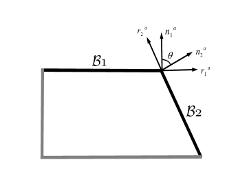
Figure 1: The timelike joint is intersected by two timelike segments $\mathcal{B}_{1}$ and $\mathcal{B}_{2}$.

Substitute (30) into (29) and make a decomposition ${\mathchar 22\relax\mkern-10.0mu\delta}A_{s}^{a}={\mathchar 22\relax\mkern-10.0mu\delta}A_{s}^{r}r_{s}^{a}+{\mathchar 22\relax\mkern-10.0mu\delta}\hat{A}_{s}^{a}$ with ${\mathchar 22\relax\mkern-10.0mu\delta}\hat{A}_{s}^{a}$ a tangent vector of the joint $\mathcal{C}$, then we have

$$\begin{aligned} &-2\delta a_{2}\,n_{2}^{a}n_{2}^{b}-{\mathchar 22\relax\mkern-10.0mu\delta}A_{2}^{r}r_{2}^{a}n_{2}^{b}-{\mathchar 22\relax\mkern-10.0mu\delta}A_{2}^{r}r_{2}^{b}n_{2}^{a}-{\mathchar 22\relax\mkern-10.0mu\delta}\hat{A}_{2}^{a}n_{2}^{b}-{\mathchar 22\relax\mkern-10.0mu\delta}\hat{A}_{2}^{b}n_{2}^{a}\\ &=-2\cos\theta\left(\sin\theta{\mathchar 22\relax\mkern-10.0mu\delta}A_{2}^{r}+\cos\theta\delta a_{2}\right)n_{1}^{a}n_{1}^{b}\\ &+\left(\cos 2\theta{\mathchar 22\relax\mkern-10.0mu\delta}A_{2}^{r}-\sin 2\theta\delta a_{2}\right)(n_{1}^{a}r_{1}^{b}+n_{1}^{b}r_{1}^{a})\\ &+2\sin\theta\left(\cos\theta{\mathchar 22\relax\mkern-10.0mu\delta}A_{2}^{r}-\sin\theta\delta a_{2}\right)r_{1}^{a}r_{1}^{b}\\ &-\sin\theta\left({\mathchar 22\relax\mkern-10.0mu\delta}\hat{A}_{2}^{a}r_{1}^{b}+{\mathchar 22\relax\mkern-10.0mu\delta}\hat{A}_{2}^{b}r_{1}^{a}\right)-\cos\theta\left({\mathchar 22\relax\mkern-10.0mu\delta}\hat{A}_{2}^{a}n_{1}^{b}+{\mathchar 22\relax\mkern-10.0mu\delta}\hat{A}_{2}^{b}n_{1}^{a}\right)\\ &=-2\delta a_{1}\,n_{1}^{a}n_{1}^{b}-\delta A_{1}^{r}r_{1}^{a}n_{1}^{b}-\delta A_{1}^{r}r_{1}^{b}n_{1}^{a}-\delta\hat{A}_{1}^{a}n_{1}^{b}-\delta\hat{A}_{1}^{b}n_{1}^{a}\,,\end{aligned}$$ (31)

which gives rise to

$$\delta a_{1} = \delta a_{2}\equiv\delta a\,,$$ (32)

$${\mathchar 22\relax\mkern-10.0mu\delta}A_{s}^{a} = \tan\theta\,\delta a\,r_{s}^{a}\,.$$ (33)

On the other hand, from the transformation (30), we can obtain

$$\cos\theta=n_{2}\cdot n_{1}\,,$$ (34)

the variation of which yields

$$\begin{aligned} -\sin\theta\,\delta\theta&=-\delta a\,n_{2}^{a}n_{1a}-{\mathchar 22\relax\mkern-10.0mu\delta}A_{2}^{a}n_{1a}+\delta an_{2}^{a}n_{1a}\\ &=-\tan\theta\,\delta a\,\sin\theta\,.\end{aligned}$$ (35)

Whence we have

$${\mathchar 22\relax\mkern-10.0mu\delta}A_{s}^{a} = \delta\theta r_{s}^{a}\,.$$ (36)

With the above preparation, the variation of the corner term can be written as

$$\begin{aligned} \delta I_{\mathcal{C}}&=2\int_{\mathcal{C}}\left({\mathchar 22\relax\mkern-10.0mu\delta}A_{1}^{a}\Psi_{1ab}dS_{1}^{b}+{\mathchar 22\relax\mkern-10.0mu\delta}A_{2}^{a}\Psi_{2ab}dS_{2}^{b}\right)\\ &=2\int_{\mathcal{C}}\left(\Psi_{1ab}{\mathchar 22\relax\mkern-10.0mu\delta}A_{1}^{a}r_{1}^{b}+\Psi_{2ab}{\mathchar 22\relax\mkern-10.0mu\delta}A_{2}^{a}r_{2}^{b}\right)dS\\ &=\int_{\mathcal{C}}\hat{\Psi}\delta\theta dS\,,\end{aligned}$$ (37)

where $\hat{\Psi}=4\Psi_{sab}r_{s}^{a}r_{s}^{b}=\psi^{abcd}\epsilon_{ab}\epsilon_{cd}$ is the Wald entropy density with the binomal defined as $\epsilon_{ab}=(n_{s}\wedge r_{s})_{ab}=2n_{[sa}r_{sb]}$, which does not depend on the choice of pairs, namely keeps invariant under the above Lorentz transformation.

The requirements $\delta\Psi_{ab}=0$ and $\delta r_{s}^{a}=0$ lead to $\delta\hat{\Psi}=0$. Accordingly, the corner term can be derived as the Wald entropy density multiplied by the rotation parameter, $i.e.$,

$$I_{\mathcal{C}}=\int_{\mathcal{C}}\hat{\Psi}\,\theta dS\,,$$ (38)

which vanishes when $\theta=0$ as it is expected to be the case.

III.3.2 Spacelike joint

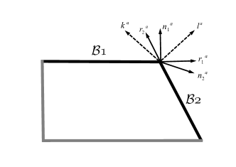
Figure 2: The spacelike joint is intersected by a spacelike segment $\mathcal{B}_{1}$ and a timelike segment $\mathcal{B}_{2}$.

As shown in Fig.2, now we consider a typical type of spacelike joint $\mathcal{C}$ intersected by a spacelike segment $\mathcal{B}_{1}$ and a timelike segment $\mathcal{B}_{2}$ . In this case, the two pairs of the normal vector $\{n_{s}^{a},r_{s}^{a}\}$ can be related to each other by the boost transformation

$$\begin{aligned} n_{2}^{a}&=r_{1}^{a}\cosh\eta-n_{1}^{a}\sinh\eta\,,\\ r_{2}^{a}&=n_{1}^{a}\cosh\eta-r_{1}^{a}\sinh\eta\,\end{aligned}$$ (39)

with $\eta$ the boost parameter. Substituting this transformation into the following equality

$$\delta g^{ab} = 2\delta a_{1}\,n_{1}^{a}n_{1}^{b}-{\mathchar 22\relax\mkern-10.0mu\delta}A_{1}^{a}n_{1}^{b}-{\mathchar 22\relax\mkern-10.0mu\delta}A_{1}^{b}n_{1}^{a}$$ (40)

$$= -2\delta a_{2}\,n_{2}^{a}n_{2}^{b}-{\mathchar 22\relax\mkern-10.0mu\delta}A_{2}^{a}n_{2}^{b}-{\mathchar 22\relax\mkern-10.0mu\delta}A_{2}^{b}n_{2}^{a}$$

at the joint $\mathcal{C}$, one can show

$$\delta a_{1} = \delta a_{2}\equiv\delta a\,,$$ (41)

$${\mathchar 22\relax\mkern-10.0mu\delta}A_{s}^{a} = \coth\eta\,\delta a\,r_{s}^{a}\,.$$ (42)

Furthermore, by virtue of the variation of $\sinh\eta=n_{1}\cdot n_{2}$, one can obtain

$${\mathchar 22\relax\mkern-10.0mu\delta}A_{s}^{a}=\delta\eta\,r_{s}^{a}\,.$$ (43)

Accordingly, the variation of the corresponding corner term can be expressed as

$$\begin{aligned} \delta I_{\mathcal{C}}&=-2\int_{\mathcal{C}}\left({\mathchar 22\relax\mkern-10.0mu\delta}A_{1}^{a}\Psi_{1ab}dS_{1}^{b}-{\mathchar 22\relax\mkern-10.0mu\delta}A_{2}^{a}\Psi_{2ab}dS_{2}^{b}\right)\\ &=-2\int_{\mathcal{C}}\left(\Psi_{1ab}{\mathchar 22\relax\mkern-10.0mu\delta}A_{1}^{a}r_{1}^{b}+\Psi_{2ab}{\mathchar 22\relax\mkern-10.0mu\delta}A_{2}^{a}r_{2}^{b}\right)dS\\ &=-\int_{\mathcal{C}}\hat{\Psi}\delta\eta dS\,,\\ \end{aligned}$$ (44)

where we have used $dS_{1}^{a}=r_{1}^{a}dS$ and $dS_{2}^{a}=-r_{2}^{a}dS$ due to the fact that $r_{1}^{a}$ is spacelike while $r_{2}^{a}$ is timelike. Whence one can obtain the corner term as

$$I_{\mathcal{C}}=-\int_{\mathcal{C}}\hat{\Psi}\eta dS\,,$$ (45)

where we have required the corner term satisfy the additivity rule, which will be documented in detail later on.

For the later convenience, we would like to re-express the boost parameter $\eta$. To this end, as shown in Fig.2, we define $l^{a}$ to be a null vector as

$$\begin{aligned} l^{a}&=A(n_{1}^{a}+r_{1}^{a})\\ &=B(n_{2}^{a}+r_{2}^{a})\,.\end{aligned}$$ (46)

Substitute the transformation (39) into it, then we have

$$B=A\left(\cosh\eta+\sinh\eta\right)=Ae^{\eta}\,,$$ (47)

which leads to a new expression for the boost parameter as

$$\eta=\ln B-\ln A=\ln\left(l\cdot n_{2}\right)-\ln\left(-l\cdot n_{1}\right)\,.$$ (48)

By the same token, in terms of another null vector

$$\begin{aligned} k^{a}&=C(n_{1}^{a}-r_{1}^{a})\\ &=D(-n_{2}^{a}+r_{2}^{a})\,,\end{aligned}$$ (49)

the boost parameter can also be written as

$$\eta=\ln\left(-k\cdot n_{1}\right)-\ln\left(-k\cdot n_{2}\right)\,.$$ (50)

III.3.3 Other joints

(a)

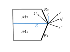
(b)

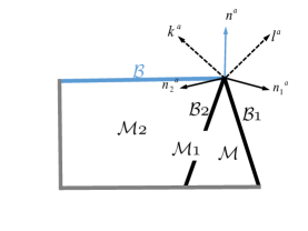
(c)

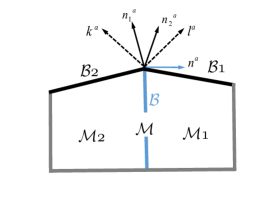
(d)

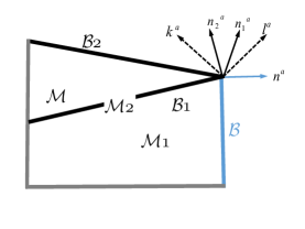
Figure 3: The corner intersected by $\mathcal{B}_{1}$ and $\mathcal{B}_{2}$ can be regarded as the addition or subtraction of two corners by introducing an auxiliary segment $\mathcal{B}$.

The additivity rule is supposed to be valid not only for the bulk term and surface term, but also for the corner term. With this in mind, one can derive the corner term for any other spacelike joint from the previous one. For instance, regarding the case (a) in Fig.3, the corresponding corner term can be obtained as a sum of two corner terms as

$$\begin{aligned} I_{\mathcal{C}_{a}}&=I_{\mathcal{B}\cap\mathcal{B}_{1}}+I_{\mathcal{B}\cap\mathcal{B}_{2}}\\ &=-\int_{\mathcal{B}\cap\mathcal{B}_{1}}\hat{\Psi}\eta_{1}dS-\int_{\mathcal{B}\cap\mathcal{B}_{2}}\hat{\Psi}\eta_{2}dS\\ &=-\int_{\mathcal{C}}\hat{\Psi}\left(\eta_{1}+\eta_{2}\right)dS\\ &=-\int_{\mathcal{C}}\hat{\Psi}\eta_{a}dS\,,\end{aligned}$$ (51)

where we have introduced an auxiliary segment $\mathcal{B}$. Note that it follows from (48) that

$$\eta_{1} = \ln\left(l\cdot n_{1}\right)-\ln\left(-l\cdot n\right)\,,$$ (52)

$$\eta_{2} = -\ln\left(l\cdot n_{2}\right)+\ln\left(-l\cdot n\right)\cdot$$ (53)

Thus we have

$$\eta_{a}=\ln\left(l\cdot n_{1}\right)-\ln\left(l\cdot n_{2}\right)\,.$$ (54)

Similarly, for the case (b), (c), and (d), the corner term can be readily expressed as minus the Wald entropy density multiplied by the boost parameter with

$$\eta_{b} = \ln\left(l\cdot n_{1}\right)-\ln\left(-l\cdot n_{2}\right)\,,$$ (55)

$$\eta_{c} = \ln\left(l\cdot n_{1}\right)-\ln\left(-l\cdot n_{2}\right)\,,$$ (56)

$$\eta_{d} = \ln\left(l\cdot n_{2}\right)-\ln\left(l\cdot n_{1}\right)\,.$$ (57)

IV Null segments

IV.1 Variation of geometric quantities

We now consider the null segment of the boundary $\mathcal{N}$, which is foliated by an outward-directed null geodesic $k^{a}=(\frac{\partial}{\partial\lambda})^{a}$ of a cross section $\mathcal{S}$. We further introduce a null vector field $l_{a}$ on $\mathcal{N}$, which is normal to $\mathcal{S}$ and satisfies $k^{a}l_{a}=-1$. With this, the metric can be decomposed as

$$g^{ab}=-k^{a}l^{b}-k^{b}l^{a}+\sigma^{ab}\,,$$ (58)

where $\sigma^{ab}$ is tangent to $\mathcal{S}$.

In what follows, we shall work with the gauge in which the location of such a null segment as well as its foliation structure keeps unchanged under the variation, $i.e.$,

$$\delta k_{a}=\delta\alpha k_{a}\,,\ \ \ \ \,\delta k^{a}=0\,,$$ (59)

which implies

$$\delta l_{a}={\mathchar 22\relax\mkern-10.0mu\delta}\beta k_{a}\,,$$ (60)

where $\delta\alpha=\delta g^{ab}k_{a}l_{b}$ and ${\mathchar 22\relax\mkern-10.0mu\delta}\beta=\frac{1}{2}\delta g^{ab}l_{a}l_{b}$. Furthermore, by $l_{a}l^{a}=0$ and $k_{a}l^{a}=-1$, one can obtain

$$\delta l^{a}=-{\mathchar 22\relax\mkern-10.0mu\delta}\beta\,k^{a}-\delta\alpha\,l^{a}+{\mathchar 22\relax\mkern-10.0mu\delta}l^{a}$$ (61)

with ${\mathchar 22\relax\mkern-10.0mu\delta}l^{a}$ tangent to $\mathcal{S}$. Whence the variation of the metric is given by

$$\begin{aligned} \delta g^{ab}&=2{\mathchar 22\relax\mkern-10.0mu\delta}\beta\,k^{a}k^{b}+\delta\alpha(k^{a}l^{b}+k^{b}l^{a})\\ &-k^{a}{\mathchar 22\relax\mkern-10.0mu\delta}l^{b}-k^{b}{\mathchar 22\relax\mkern-10.0mu\delta}l^{a}+\delta\sigma^{ab}\,.\end{aligned}$$ (62)

The geodesic equation reads

$$k^{a}\nabla_{a}k^{b}=\kappa\,k^{b}\,,$$ (63)

where $\kappa$ measures the failure of $\lambda$ to be an affine parameter. Whence we have the following two expressions for the variation of $\kappa$ as

$$\delta\kappa = -\delta\left(l^{a}k^{b}\nabla_{b}k_{a}\right)=k^{a}\nabla_{a}\delta\alpha+\delta\Gamma^{c}{}_{ab}l^{a}k^{b}k_{c}\,,$$ (64)

$$\delta\kappa = -\delta\left(l_{a}k^{b}\nabla_{b}k^{a}\right)=-\delta\Gamma^{a}{}_{bc}l_{a}k^{b}k^{c}\,,$$ (65)

which give rise to

$$\delta\Gamma^{c}{}_{ab}l^{a}k^{b}k_{c}-\delta\Gamma^{a}{}_{bc}l_{a}k^{b}k^{c}=2\delta\kappa-k^{a}\nabla_{a}\delta\alpha\,.$$ (66)

IV.2 Surface term on the boundary

For the null segment $\mathcal{N}$, the boundary term in the variation of the bulk action can be expressed as

$$\begin{aligned} &\int_{\mathcal{N}}{\mathchar 22\relax\mkern-10.0mu\delta}v^{a}d\Sigma_{a}=\int_{\mathcal{N}}k_{a}{\mathchar 22\relax\mkern-10.0mu\delta}v^{a}d\lambda dS\\ &=\int_{\mathcal{N}}\left[2k_{c}{{\psi}_{a}}{}^{bcd}\delta{\Gamma^{a}}_{bd}+2k_{c}\delta g_{bd}\nabla_{a}{\psi}^{abcd}\right]d\lambda dS\,.\end{aligned}$$ (67)

By insertion of (58), we have

$$\begin{aligned} &k_{c}{{\psi}_{a}}{}^{bcd}\delta{\Gamma^{a}}_{bd}=\frac{1}{4}\hat{\Psi}\left(\delta\Gamma^{a}{}_{bc}k_{a}k^{b}l^{c}-\delta\Gamma^{c}{}_{ab}k^{a}k^{b}l_{c}\right)\\ &+k^{a}\psi_{{acdf}}\sigma^{{bc}}\sigma^{{ed}}\sigma^{{hf}}\nabla_{h}\delta g_{{be}}-k^{a}k^{b}\psi_{{bcdf}}l^{c}\sigma^{{ed}}\sigma^{{hf}}\nabla_{h}{\delta g}_{{ae}}\\ &+k^{a}k^{b}k^{c}\psi_{{cedf}}l^{d}l^{e}\sigma^{{fh}}\left(\nabla_{h}{\delta g}_{{ab}}-\nabla_{b}{\delta g}_{{ah}}\right)\\ &+k^{a}k^{b}\psi_{{bdcf}}k^{c}l^{d}l^{e}\sigma^{{fh}}\left(\nabla_{a}{\delta g}_{{eh}}+\nabla_{h}{\delta g}_{{ae}}-2\nabla_{e}{\delta g}_{{ah}}\right)\\ &+k^{a}\psi_{{adbf}}k^{b}l^{c}\sigma^{{ed}}\sigma^{{hf}}\left(\nabla_{c}{\delta g}_{{eh}}-\nabla_{h}{\delta g}_{{ec}}\right)\\ &+k^{a}k^{b}\psi_{{bdcf}}l^{c}\sigma^{{ed}}\sigma^{{hf}}\left(\nabla_{a}{\delta g}_{{eh}}-\nabla_{h}{\delta g}_{{ea}}\right)\,,\end{aligned}$$ (68)

where $\hat{\Psi}=4\psi_{abcd}k^{a}l^{b}k^{c}l^{d}=\psi^{abcd}\epsilon_{ab}\epsilon_{cd}$ with the binormal given by $\epsilon_{ab}=(k\wedge l)_{ab}$. Substituting (66) and (62) into the above expression and make a straightforward but tedious calculation, one can obtain

$$\begin{aligned} &\int_{\mathcal{N}}{\mathchar 22\relax\mkern-10.0mu\delta}v^{a}d\Sigma_{a}=\int_{\mathcal{N}}\hat{\Psi}\delta\kappa d\lambda dS\\ &-\int_{\mathcal{N}}\frac{d}{d\lambda}\left[\left(\frac{1}{2}\hat{\Psi}\delta\alpha-2k^{a}k^{b}\psi_{acbd}l^{c}{\mathchar 22\relax\mkern-10.0mu\delta}l^{d}\right)dS\right]d\lambda\\ &-2\int_{\mathcal{N}}\left[\tilde{D}_{e}\left(k^{a}k^{b}l^{c}\sigma^{de}\psi_{acbd}\delta\alpha-k^{a}k^{b}\sigma^{ed}\psi_{acbd}{\mathchar 22\relax\mkern-10.0mu\delta}l^{c}\right)\right]d\lambda dS\,,\end{aligned}$$ (69)

where we have already used the condition $\delta\sigma^{ab}=0$ with $\tilde{D}_{a}$ the covariant derivative operator on $\mathcal{S}$. Below we shall focus on the case in which $\partial\mathcal{S}=0$. Then the last term in (69) vanishes, which leads to

$$\begin{aligned} &\int_{\mathcal{N}}{\mathchar 22\relax\mkern-10.0mu\delta}v^{a}d\Sigma_{a}=\delta\left[\int_{\mathcal{N}}\hat{\Psi}\kappa d\lambda dS\right]\\ &-\int_{\partial\mathcal{N}^{+}}\left(\frac{1}{2}\hat{\Psi}\delta\alpha-2k^{a}k^{b}\psi_{acbd}l^{c}{\mathchar 22\relax\mkern-10.0mu\delta}l^{d}\right)dS\\ &+\int_{\partial\mathcal{N}^{-}}\left(\frac{1}{2}\hat{\Psi}\delta\alpha-2k^{a}k^{b}\psi_{acbd}l^{c}{\mathchar 22\relax\mkern-10.0mu\delta}l^{d}\right)dS\end{aligned}$$ (70)

where we have used $\delta\hat{\Psi}=0$. Thus the surface term from the null segment $\mathcal{N}$ is given by

$$I_{\text{surf}}=-\int_{\mathcal{N}}\hat{\Psi}\kappa d\lambda dS\,.$$ (71)

On the other hand, if the joint on the boundary is intersected by one null and another non-null segment, the variation of the corner term can be obviously expressed as

$$\begin{aligned} \delta I_{\text{corner}}&=\pm\int_{\mathcal{C}_{s\pm}}\left(\frac{1}{2}\hat{\Psi}\delta\alpha-2k^{a}k^{b}\psi_{acbd}l^{c}{\mathchar 22\relax\mkern-10.0mu\delta}l^{d}\right)dS\\ &+2\int_{\mathcal{C}_{s\pm}}\left(\varepsilon_{s}{\mathchar 22\relax\mkern-10.0mu\delta}A_{s}^{a}\Psi_{sab}dS_{s}^{b}\right)\,.\end{aligned}$$ (72)

IV.3 Corner term on the boundary

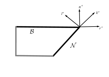
Figure 4: The spacelike joint is interjected by a null segment and a spacelike segment.

IV.3.1 Joint by a null and a spacelike segment

As illustrated in Fig.4, we first consider the joint which is intersected by a spacelike segment $\mathcal{B}$ and a null segment $\mathcal{N}$. In this case, there exists a transformation at the joint $\mathcal{C}$, from the pair of normals $\{n^{a},r^{a}\}$ to the double nulls $\{k^{a},l^{a}\}$

$$\begin{aligned} k^{a}&=e^{\chi}\left(n^{a}+r^{a}\right)\,,\\ l^{a}&=\frac{1}{2}e^{-\chi}\left(n^{a}-r^{a}\right)\,\end{aligned}$$ (73)

with $\chi$ a scaling factor. Substituting the inverse of this transformation into the following variational identity

$$\begin{aligned} &\delta g^{ab}=2\delta a\,n^{a}n^{b}-{\mathchar 22\relax\mkern-10.0mu\delta}A^{a}n^{b}-{\mathchar 22\relax\mkern-10.0mu\delta}A^{b}n^{a}\\ &=2{\mathchar 22\relax\mkern-10.0mu\delta}\beta\,k^{a}k^{b}+\delta\alpha(k^{a}l^{b}+k^{b}l^{a})-k^{a}{\mathchar 22\relax\mkern-10.0mu\delta}l^{b}-k^{b}{\mathchar 22\relax\mkern-10.0mu\delta}l^{a}\end{aligned}$$ (74)

at the joint with $h^{ab}$ and $\sigma^{ab}$ fixed, we can obtain

$$\begin{aligned} &\delta g^{ab}=2{\mathchar 22\relax\mkern-10.0mu\delta}\beta\,k^{a}k^{b}+\delta\alpha(k^{a}l^{b}+k^{b}l^{a})-k^{a}{\mathchar 22\relax\mkern-10.0mu\delta}l^{b}-k^{b}{\mathchar 22\relax\mkern-10.0mu\delta}l^{a}\\ &=\frac{e^{-2\chi}}{2}\left(\delta a-{\mathchar 22\relax\mkern-10.0mu\delta}A^{r}\right)k^{a}k^{b}+2e^{2\chi}(\delta a+{\mathchar 22\relax\mkern-10.0mu\delta}A^{r})l^{a}l^{b}\\ &+\delta a(k^{b}l^{a}+k^{a}l^{b})-\frac{e^{-\chi}}{2\sqrt{2}}\left(k^{a}{\mathchar 22\relax\mkern-10.0mu\delta}\hat{A}^{b}+k^{b}{\mathchar 22\relax\mkern-10.0mu\delta}\hat{A}^{a}\right)\\ &-\sqrt{2}e^{\chi}\left(l^{a}{\mathchar 22\relax\mkern-10.0mu\delta}\hat{A}^{b}+l^{b}{\mathchar 22\relax\mkern-10.0mu\delta}\hat{A}^{a}\right)\,,\end{aligned}$$ (75)

which gives

$$\begin{aligned} {\mathchar 22\relax\mkern-10.0mu\delta}A^{r}&=-\,\delta a\ \ \ \ ,\ \ \ {\mathchar 22\relax\mkern-10.0mu\delta}\hat{A}^{a}={\mathchar 22\relax\mkern-10.0mu\delta}l^{a}=0\,,\\ \delta\alpha&=\delta a\ \ \ \ \ \ ,\ \ \ \ {\mathchar 22\relax\mkern-10.0mu\delta}\beta=\frac{1}{2}e^{-2\chi}\delta a\,.\end{aligned}$$ (76)

Furthermore, by virtue of the variation of $e^{\chi}=-n_{a}k^{a}$, one can obtain

$$\delta a=\delta\chi=\delta\ln\left(-n\cdot k\right)\,.$$ (77)

With the above preparation, the variation of the corner term can be written as

$$\begin{aligned} \delta I_{\mathcal{C}}=\int_{\mathcal{C}}\hat{\Psi}\delta\chi dS\end{aligned}$$ (78)

which gives the corner term as

$$I_{\mathcal{C}}=\int_{\mathcal{C}}\hat{\Psi}\,\chi dS$$ (79)

with

$$\chi=\ln\left(-n\cdot k\right)\,.$$ (80)

IV.3.2 Joint intersected by double null segments

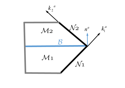
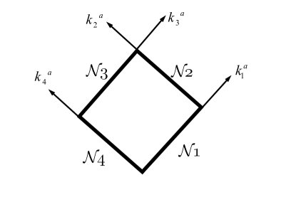
Figure 5: The joint is intersected by double null segments can be obtained by the additivity rule.

With the corner term obtained before, one can readily derive the corner term for any other type of joint by the additivity rule. As a demonstration and for the later calculations as well, we would like to derive the corner term for the joint intersected by double null segments. As illustrated in the left panel of Fig.5, we first add an auxiliary spacelike segment $\mathcal{B}$, which divides the corner into two parts. Then by the additivity rule, we have

$$\begin{aligned} I_{\mathcal{C}}&=\,\int_{\mathcal{C}}\hat{\Psi}\ln\left(-n\cdot k_{1}\right)dS+\,\int_{\mathcal{C}}\hat{\Psi}\ln\left(-n\cdot k_{2}\right)dS\\ &=\int_{\mathcal{C}}\hat{\Psi}\left[\ln\left(-n\cdot k_{1}\right)+\ln\left(-n\cdot k_{2}\right)\right]dS\,\\ &=\int_{\mathcal{C}}\hat{\Psi}\ln(-\frac{1}{2}k_{1}\cdot k_{2})dS\,.\end{aligned}$$ (81)

Whence one can readily write down the corner term for the four joints in the right panel of Fig.5 as

$$\begin{aligned} &I_{\text{corner}}=I_{\mathcal{C}_{12}}+I_{\mathcal{C}_{23}}+I_{\mathcal{C}_{34}}+I_{\mathcal{C}_{41}}\\ &=\int_{\mathcal{C}_{12}}\hat{\Psi}\,\ln(-\frac{1}{2}k_{1}\cdot k_{2})dS-\int_{\mathcal{C}_{23}}\hat{\Psi}\,\ln(-\frac{1}{2}k_{2}\cdot k_{3})dS\\ &+\int_{\mathcal{C}_{34}}\hat{\Psi}\,\ln(-\frac{1}{2}k_{3}\cdot k_{4})dS-\int_{\mathcal{C}_{41}}\hat{\Psi}\,\ln(-\frac{1}{2}k_{4}\cdot k_{1})dS\,.\end{aligned}$$ (82)

IV.4 Counter term on the boundary

Note that the surface term as well as the corner term from the null segment depends on the parametrization of the null generator. In order to eliminate this ambiguity, we can introduce a counter term

$$I_{\text{ct}}=-\int_{\mathcal{N}}\hat{\Theta}\ln\left(l_{\text{ct}}\Theta\right)d\lambda dS\,,$$ (83)

where $\hat{\Theta}=\nabla_{a}(k^{a}\hat{\Psi})=\frac{1}{\sqrt{\sigma}}\partial_{\lambda}(\hat{\Psi}\sqrt{\sigma})$ and $\Theta=\nabla_{a}k^{a}=\frac{1}{\sqrt{\sigma}}\partial_{\lambda}(\sqrt{\sigma})$ is the expansion scalar of the null generator with $l_{ct}$ an arbitrary length scale. To show this, let us consider the reparametrization $\frac{d\bar{\lambda}}{d\lambda}=e^{-\beta}$, which gives

$$\begin{aligned} &\bar{k}^{a}=e^{\beta}k^{a}\,,\ \ \ \ \bar{\kappa}=e^{\beta}\left(\kappa+\partial_{\lambda}\beta\right)\,,\\ &\bar{\Theta}=e^{\beta}\Theta\,,\ \ \ \ \ \bar{\hat{\Theta}}=e^{\beta}\hat{\Theta}\,.\end{aligned}$$ (84)

As a result, we have

$$\begin{aligned} &\bar{I}_{\text{surf}}+\bar{I}_{\text{corner}}=I_{\text{surf}}+I_{\text{corner}}\\ &-\int_{\mathcal{N}}\hat{\Psi}(\partial_{\lambda}\beta)d\lambda dS+\int_{\partial\mathcal{N}^{+}}\hat{\Psi}\beta dS-\int_{\partial\mathcal{N}^{-}}\hat{\Psi}\beta dS\\ &=I_{\text{surf}}+I_{\text{corner}}+\int_{\mathcal{N}}\frac{\beta}{\sqrt{\sigma}}\partial_{\lambda}(\hat{\Psi}\sqrt{\sigma})d\lambda dS\,,\\ \end{aligned}$$ (85)

and

$$\bar{I}_{\text{ct}}=I_{\text{ct}}-\int_{\mathcal{N}}\frac{\beta}{\sqrt{\sigma}}\partial_{\lambda}(\hat{\Psi}\sqrt{\sigma})d\lambda dS\,,$$ (86)

which implies

$$I_{\text{surf}}+I_{\text{corner}}+I_{\text{ct}}$$ (87)

is invariant under the above reparametrization.

V Application: Case studies for action growth rate

V.1 Case 1: SAdS spacetime

We shall apply our above result to calculate the action growth rate of the WDW patch in the SAdS spacetime for $F(R)$ gravity and critical gravity, respectively. The SAdS metric is obtained originally as a solution to Einstein equation with a negative cosmological constant, $i.e.$,

$$R_{ab}=-\frac{d+1}{L^{2}}g_{ab}$$ (88)

with $L$ the AdS curvature radius. Its $(d+2)$-dimensional expression is given by

$$ds^{2}=-f(r)dt^{2}+\frac{dr^{2}}{f(r)}+r^{2}d\Omega_{d,k}^{2}\,,$$ (89)

where $f(r)=\frac{r^{2}}{L^{2}}+k-\frac{\omega^{d-1}}{r^{d-1}}$ is the blackening factor, and $k=\{+1,0,-1\}$ denotes the $d$-dimensional spherical, planar, and hyperbolic geometry, individually. The horizon $r=r_{h}$ lies in the location where $f(r_{h})=0$.

As illustrated in the Penrose diagram of the SAdS spacetime Fig.6, $I(t_{L},t_{R})$, denoted as the action for the WDW patch determined by the time slices on the left and right AdS boundaries, is invariant under the time translation, i.e., $I(t_{L}+\delta t,t_{R}-\delta t)=I(t_{L},t_{R})$. Thus the action growth can be computed as $\delta I=I(t_{0}+\delta t,t_{1})-I(t_{0},t_{1})$, where the time on the right boundary has been fixed. To regulate the divergence near the AdS boundary, a cut-off surface $r=r_{\text{max}}$ is introduced. In addition, we also introduce a spacelike surface $r=r_{\text{min}}$ to avoid running into the spacelike singularity inside of the SAdS black hole. As such, we shall focus on the situation in which the boundary consists solely of null and spacelike segments only with spacelike joints. In addition, for simplicity we shall adopt the affine parameter for the null generator of null segments such that the surface term vanishes for null segments. With this in mind, we have

$$\begin{aligned} \delta I&=I_{\mathcal{M}_{1}}-I_{\mathcal{M}_{2}}+I_{\Sigma}+I_{\mathcal{C}_{1}}-I_{\mathcal{C}_{2}}+\delta I_{\text{ct}}\,.\\ \end{aligned}$$ (90)

Here $\mathcal{M}_{1}$ is bounded by $u=t_{0}$, $u=t_{0}+\delta t$,$v=t_{0}+\delta t$, and $r=r_{\text{min}}$. $\mathcal{M}_{2}$ is bounded by $u=t_{0}$, $v=t_{0}$, $v=v_{0}+\delta t$, and $u=t_{1}$. The null coordinates are defined as $u=t+r^{*}(r)$ and $v=t-r^{*}(r)$ with $r^{*}(r)=\int\frac{dr}{f}$.

V.1.1 $F(R)$ gravity

For a general $F(R)$ gravity, the equation of motion reads

$$F^{\prime}(R)R_{ab}-\frac{1}{2}F(R)g_{ab}-(\nabla_{a}\nabla_{b}-g_{ab}\nabla^{c}\nabla_{c})F^{\prime}(R)=0\,,$$

and the auxiliary field as well as its decedents can be expressed as

$$\begin{aligned} \psi^{abcd}&=\frac{1}{2}\left(g^{ac}g^{bd}-g^{ad}g^{bc}\right)F^{\prime}(R)\,,\\ \Psi_{ab}&=-\frac{1}{2}h_{ab}F^{\prime}(R)\,,\\ \hat{\Psi}&=-2F^{\prime}(R)\,.\end{aligned}$$ (92)

Whence the full on-shell action can be simplified as

$$\begin{aligned} &I=I_{\text{bulk}}+I_{\text{surf}}+I_{\text{corner}}+I_{\text{ct}}\\ &=\int_{\mathcal{M}}d^{d+2}x\sqrt{-g}F(R)-2\sum_{s}\left(\int_{\mathcal{B}_{s}}KF^{\prime}(R)d\Sigma\right)\\ &-2(-1)^{\lambda}\int_{\mathcal{C}_{\lambda}}\,c_{\lambda}F^{\prime}(R)dS-\int_{\mathcal{N}}\hat{\Theta}\ln\left(l_{\text{ct}}\Theta\right)d\lambda dS\,.\end{aligned}$$ (93)

In what follows, we shall consider the special case, in which there exists an $R_{0}$ such that

$$F(R_{0})=\frac{2R_{0}}{d+2}F^{\prime}(R_{0})\,,$$ (94)

where the prime denotes the derivative with respect to $R$. As such, (88) with $L^{2}=-\frac{(d+1)(d+2)}{R_{0}}$ satisfies the above equation of motion. Accordingly, the SAdS metric can be regarded as its solution.

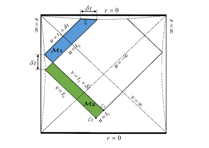
Figure 6: Wheeler-DeWitt patches of a Schwarzschild-AdS black hole.

With the above preparation, now let us use (90) to calculate the action growth rate in our $F(R)$ gravity. So we only need to keep the first order of $\delta t$ below for each term in (90). First, with the $(u,r)$ coordinates, we have

$$\begin{aligned} I_{\mathcal{M}_{1}}&=F(R_{0})\Omega_{d,k}\int_{t_{0}}^{t_{0}+\delta t}du\int_{r_{\text{min}}}^{\rho(u)}r^{d}dr\\ &=\frac{F(R_{0})\Omega_{d,k}}{d+1}r_{\text{max}}^{d+1}\delta t\,,\end{aligned}$$ (95)

where $r=\rho(u)$ is the solution to the equation $v(u,r)=t_{0}+\delta t$ and $r_{\text{min}}$ has been set to zero in the end. Similarly, with the $(v,r)$ coordinates, we have

$$\begin{aligned} I_{\mathcal{M}_{2}}&=F(R_{0})\Omega_{d,k}\int_{t_{0}}^{t_{0}+\delta t}dv\int_{\rho_{1}(v)}^{\rho_{0}(v)}r^{d}dr\\ &=\frac{F(R_{0})\Omega_{d,k}}{d+1}\left(r_{\text{max}}^{d+1}-r_{1}^{d+1}\right)\delta t\,,\end{aligned}$$ (96)

where $r=\rho_{0}(v)$ is the solution to the equation $u(v,r)=t_{0}$ and $r=\rho_{1}(v)$ is the solution to the equation $u(v,r)=t_{1}$ with $r_{1}$ the $r$ coordinate of $\mathcal{C}_{1}$. Thus the difference between $I_{\mathcal{M}_{1}}$ and $I_{\mathcal{M}_{2}}$

$$I_{\mathcal{M}_{1}}-I_{\mathcal{M}_{2}}=\frac{F(R_{0})\Omega_{d,k}}{d+1}r_{1}^{d+1}\delta t\,.$$ (97)

For the surface term, we have

$$\begin{aligned} I_{\Sigma}&=-2F^{\prime}(R_{0})\int_{\mathcal{S}}Kd\Sigma\\ &=(d+1)F^{\prime}(R_{0})\Omega_{d,k}\omega^{d-1}\delta t,\end{aligned}$$ (98)

where we have used the expression $K=-\frac{1}{r^{d}}\frac{d}{dr}\left(r^{d}\sqrt{-f}\right)$ for the spacelike surface $r=r_{\text{min}}$ and let $r_{\text{min}}\to 0$ in the end.

In order to write down the explicit expression for the difference between the two corner terms from $\mathcal{C}_{1}$ and $\mathcal{C}_{2}$, we shall choose $k_{1a}=\nabla_{a}u$ and $k_{2a}=-\nabla_{a}v$. Note that $k_{1}\cdot k_{2}=-\frac{2}{f}$. Then by (82), we can obtain

$$\begin{aligned} &I_{\mathcal{C}_{1}}-I_{\mathcal{C}_{2}}=F^{\prime}(R_{0})\Omega_{d,k}\\ &\times\left[r_{1}^{d}f^{\prime}(r_{1})+d\,r_{1}^{d-1}f(r_{1})\ln\left(-f(r_{1})\right)\right]\delta t\,,\end{aligned}$$ (99)

where we have used

$$\delta r=r_{1}-r_{2}=-\frac{1}{2}f(r_{1})\delta t\,$$ (100)

with $r_{2}$ the $r$ coordinate of $\mathcal{C}_{2}$.

In the SAdS spacetime, the counter term can be expressed as

$$I_{\text{ct}}=2F^{\prime}(R_{0})\int_{\mathcal{N}}\Theta\ln(l_{\text{ct}}\Theta)d\lambda dS\,.$$ (101)

By the translation symmetry, there are only two null segments contributing to the action growth. The first one comes from the null segment $u=t_{1}$ with $r$ as the affine parameter, $i.e.$, $k_{1}^{a}=\left(\frac{\partial}{\partial r}\right)^{a}$, which gives rise to the expansion $\Theta=\frac{d}{r}$. As a result, the corresponding counter term can be written as

$$\begin{aligned} &I_{\text{ct}}^{(1)}=2d\Omega_{d,k}F^{\prime}(R_{0})\int_{r_{2}}^{r_{\text{max}}}dr\,r^{d-1}\ln\left(\frac{dl_{\text{ct}}}{r}\right)\\ &=2\Omega_{d,k}F^{\prime}(R_{0})\times\\ &\left[r_{\text{max}}^{d}\ln\left(\frac{dl_{\text{ct}}}{r_{\text{max}}}\right)-r_{2}^{d}\ln\left(\frac{dl_{\text{ct}}}{r_{2}}\right)+\frac{1}{d}\left(r_{\text{max}}^{d}-r_{2}^{d}\right)\right]\,.\end{aligned}$$ (102)

Obviously, as to the counter term from the second null segment $v=t_{0}$, we have $I_{\text{ct}}^{(2)}=I_{\text{ct}}^{(1)}$. By (100), the growth of the counter term can be written as

$$\begin{aligned} \delta I_{\text{ct}}=2d\Omega_{d,k}F^{\prime}(R_{0})f(r_{1})r_{1}^{d-1}\ln\left(\frac{dl_{\text{ct}}}{r_{1}}\right)\delta t\,.\end{aligned}$$ (103)

Then summing all the previous terms, we end up with

$$\begin{aligned} \delta I&=\Omega_{d,k}F^{\prime}(R_{0})\left[-2\frac{r_{1}^{d+1}}{L^{2}}+(d+1)\omega^{d-1}\right.\\ &\left.+r_{1}^{d}f^{\prime}(r_{1})+d\,r_{1}^{d-1}f(r_{1})\ln\left(\frac{-f(r_{1})d^{2}l_{\text{ct}}^{2}}{r_{1}^{2}}\right)\right]\delta t\\ &=2d\,\Omega_{d,k}F^{\prime}(R_{0})\omega^{d-1}\\ &\times\left[1+\frac{1}{2}\left(\frac{r_{1}}{\omega}\right)^{d-1}f(r_{1})\ln\left(\frac{-f(r_{1})d^{2}l_{\text{ct}}^{2}}{r_{1}^{2}}\right)\right]\delta t\\ &=2M_{F}\left[1+\frac{1}{2}\left(\frac{r_{1}}{\omega}\right)^{d-1}f(r_{1})\ln\left(\frac{-f(r_{1})d^{2}l_{\text{ct}}^{2}}{r_{1}^{2}}\right)\right]\delta t\,,\end{aligned}$$ (104)

where

$$M_{F}=\Omega_{d,k}d\omega^{d-1}F^{\prime}(R_{0})\,$$ (105)

is the ADM massDKH . As a result, the action growth rate is given by

$$\dot{I}=2M_{F}\left[1+\frac{1}{2}\left(\frac{r_{1}}{\omega}\right)^{d-1}f(r_{1})\ln\left(\frac{-f(r_{1})d^{2}l_{\text{ct}}^{2}}{r_{1}^{2}}\right)\right]\,,$$

which reduces to

$$\dot{I}=2M_{F}\,,$$ (107)

in the late time limit with $r_{1}\to r_{h}$. It is noteworthy that this late time behavior is also obtained by different approaches in AFNV ; GWLL ; WYY .

V.1.2 Critical gravity

Now let us move onto the critical gravity. The original bulk action is given byAFNV ; LP ,

$$\begin{aligned} &I_{\text{bulk}}=\int_{\mathcal{M}}d^{d+2}x\sqrt{-g}\\ &\times\left[R-2\Lambda-\frac{1}{m^{2}}\left(R^{ab}R_{ab}-\frac{d+2}{4(d+1)}R^{2}\right)\right]\,,\end{aligned}$$ (108)

where $m$ is a dimensionful parameter. Whence the corresponding equation of motion can be obtained as

$$\left[8\Lambda m^{2}+8d\Lambda m^{2}+4(d+1)\left(R_{{cd}}R^{{cd}}-m^{2}R\right)\right.$$

$$\left.+(d+2)\left(4\nabla_{c}\nabla^{c}R-R^{2}\right)-8(d+1)\nabla_{c}\nabla_{d}R^{{cd}}\right]g_{{ab}}$$

$$+4\left[R_{{ab}}\left(2(d+1)m^{2}+(d+2)R\right)-4(d+1)R_{{bc}}R^{c}{}_{a}\right]$$

$$+4\left[-(d+2)\nabla_{a}\nabla_{b}R+2(d+1)\nabla_{a}\nabla_{c}R^{c}{}_{b}\right.$$

$$\left.+2(d+1)\nabla_{b}\nabla_{c}R^{c}{}_{a}{}-2(d+1)\nabla_{c}\nabla^{c}R_{{ab}}\right]=0\,,$$

and the auxiliary field as well as its decedents reads

$$\psi^{abcd}=\left(1+\frac{2+d}{2(1+d)m^{2}}R\right)g^{c[a}g^{b]d}$$

$$-\frac{1}{m^{2}}R^{a[c}g^{d]b}-\frac{1}{m^{2}}R^{c[b}g^{a]d}\,,$$

$$\Psi_{ab}=-\frac{1}{2}\left(1+\frac{2+d}{2(1+d)m^{2}}R\right)h_{ab}$$ (110)

$$-\frac{1}{2m^{2}}\left[R_{cd}n^{c}n^{d}g_{ab}-R_{ab}-n^{c}\left(n_{a}R_{bc}+n_{b}R_{ac}\right)\right]\,,$$

$$\hat{\Psi}=-2+\frac{1}{m^{2}}\left(2R_{ab}r^{a}r^{b}-2R_{ab}n^{a}n^{b}-\frac{d+2}{d+1}R\right)\,.$$

It is not hard to show that with

$$\Lambda=\frac{d(d+1)\left(d^{2}-2d-4L^{2}m^{2}\right)}{8L^{4}m^{2}}\,,$$ (111)

(88) satisfies the equation of motion. So in this case, the SAdS metric is also the solution to the critical gravity. With this solution, one can obtain

$$\begin{aligned} &I_{\text{bulk}}=-2\frac{d+1}{L^{2}}\left(1-\frac{d^{2}}{2L^{2}m^{2}}\right)\int_{\mathcal{M}}d^{d+2}x\sqrt{-g}\,,\\ &\Psi_{ab}=-\frac{1}{2}\left(1-\frac{d^{2}}{2L^{2}m^{2}}\right)h_{ab}\,,\\ &\hat{\Psi}=-2\left(1-\frac{d^{2}}{2L^{2}m^{2}}\right)\,.\end{aligned}$$ (112)

Following the same calculation as $F(R)$ gravity, one can easily obtain the action growth rate for the critical gravity as

$$\dot{I}=2M_{C}\left[1+\frac{1}{2}\left(\frac{r_{1}}{\omega}\right)^{d-1}f(r_{1})\ln\left(\frac{-f(r_{1})d^{2}l_{\text{ct}}^{2}}{r_{1}^{2}}\right)\right]\,,$$

where

$$\begin{aligned} M_{C}=d\,\Omega_{d,k}\omega^{d-1}\left(1-\frac{d^{2}}{2L^{2}m^{2}}\right)\,\end{aligned}$$ (114)

is the ADM mass for the critical gravityLP . The late time action growth rate is the same as that obtained in AFNV by using the approach developed in BRSSZ1 ; BRSSZ2 .

V.2 Case 2: The asymptotically AdS black hole for the critical Einsteinian cubic gravity

In this subsection, we consider the $4$-dimensional the critical Einsteinian cubic gravity. The corresponding bulk action is given byBC

$$\begin{aligned} I_{\text{bulk}}&=\int_{\mathcal{M}}d^{4}x\sqrt{-g}F\\ &=\int_{\mathcal{M}}d^{4}x\sqrt{-g}\left(R-2\Lambda+\lambda\mathcal{P}\right)\,,\end{aligned}$$ (115)

where the cubic invariant polynomial term $\mathcal{P}$ of the Riemann tensor reads

$$\begin{aligned} \mathcal{P}&=12R_{acbd}R^{cedf}R_{e}{}^{a}{}_{f}{}^{b}+R_{ab}{}^{cd}R_{cd}{}^{ef}R_{ef}{}^{ab}\\ &-12R_{abcd}R^{ac}R^{bd}+8R_{a}{}^{b}R_{b}{}^{c}R^{a}{}_{c}\end{aligned}$$ (116)

with $\lambda$ the coupling constant.

In terms of the auxiliary field

$$\begin{aligned} &\psi_{abcd}=\frac{1}{2}\left(g_{ac}g_{bd}-g_{ad}g_{bc}\right)+6\lambda\left(R_{ad}R_{bc}\right.\\ &-R_{ac}R_{bd}+g_{bd}R_{a}{}^{e}R_{ce}-g_{ad}R_{b}{}^{e}R_{ce}\\ &-g_{bc}R_{a}{}^{e}R_{de}+g_{ac}R_{b}{}^{e}R_{de}-g_{bd}R^{ef}R_{aecf}\\ &+g_{bc}R^{ef}R_{aedf}+g_{ad}R^{ef}R_{becf}-g_{ac}R^{ef}R_{bedf}\\ &-3R_{a}{}^{e}{}_{d}{}^{f}R_{becf}+3R_{a}{}^{e}{}_{c}{}^{f}R_{bedf}+\frac{1}{2}R_{ab}{}^{ef}R_{cdef})\,,\end{aligned}$$ (117)

the equation of motion can be expressed as

$$\begin{aligned} \psi_{acde}R_{b}{}^{cde}-\frac{1}{2}g_{ab}F-2\nabla^{c}\nabla^{d}\psi_{acdb}=0\,.\end{aligned}$$ (118)

As shown in FHML , when the parameters satisfies the following critical relation

$$\Lambda=-\frac{2}{L^{2}}\,,\ \ \ \ \lambda=-\frac{L^{4}}{24}\,,$$ (119)

the above equation of motion admits a static asymptotically AdS black hole solution, whose line element can be written as

$$ds^{2}=-f(r)dt^{2}+\frac{dr^{2}}{f(r)}+r^{2}d\Omega_{2,k}^{2}$$ (120)

with the blackening factor

$$f(r)=\frac{r^{2}}{L^{2}}+k-\mu\,.$$ (121)

Then following the exact same procedure, one can obtain

$$I_{\mathcal{M}_{1}} -I_{\mathcal{M}_{2}}=4\Omega_{2,k}r_{1}\left(\mu-\frac{r_{1}^{2}}{L^{2}}\right)\delta t\,.$$ (122)

By using (26), one can further find that the surface term of $\Sigma$ vanishes. In addition, the straightforward calculation gives rise to the following corner term

$$\begin{aligned} &I_{\mathcal{C}_{1}}-I_{\mathcal{C}_{2}}=4\Omega_{2,k}r_{1}\\ &\times\left[\left(\frac{r_{1}^{2}}{L^{2}}-\mu\right)+f(r_{1})\ln\left(-f(r_{1})\right)\right]\delta t\,.\end{aligned}$$ (123)

At last, the counter term contribution of the null segments can be obtained as

$$\delta I_{\text{ct}}=8\Omega_{2,k}r_{1}f(r_{1})\ln\left(\frac{2l_{\text{ct}}}{r_{1}}\right)\delta t\,,$$ (124)

where we have used $\hat{\Theta}=-\frac{8}{r}$. By summing all the previous terms, we end up with

$$\begin{aligned} \dot{I}=4\Omega_{2,k}r_{1}f(r_{1})\ln\left(-\frac{4f(r_{1})l_{\text{ct}}^{2}}{r_{1}^{2}}\right)\,.\end{aligned}$$ (125)

In the late time limit, the action growth rate apparently vanishes. However, this late time behavior still saturates the Lloyd bound because the mass of this black hole also vanishesFHML .

VI Conclusion

We have presented a complete discussion of the variational problem for $F($Riemann$)$ gravity with a non-smooth boundary. In order to give rise to a well posed variational principle, we must supplement the surface term and corner term to the bulk action. Following the method developed in LMPS , we obtain a general formula for the boundary term, where the corner term can be obtained by integrating the Wald entropy density weighted by a transformation parameter between the two intersected segments. When the involved segment is null, we are also required to add a counter term to make the full boundary term invariant under the reparametrization.

Then motivated by the CA conjecture, we apply the resulting full action to evaluate the full time action growth rate of the WDW patch in the SAdS spacetime for the $F(R)$ gravity and critical gravity, as well as in an asympotically AdS black hole for the critical Einsteinian cubic gravity. For the $F(R)$ and critical gravity, the late time action growth rate shares exactly the same behavior as those obtained by other approaches. For the critical Einsteinian cubic gravity, we find that the late time action growth rate vanishes but still saturates the Lloyd bound.

- (1) R. H. Gowdy, Phys. Rev. D 2, 2774(1970).
- (2) J. W. York, Phys. Rev. Lett. 28, 1082(1972).
- (3) G. W. Gibbons and S. W. Hawking, Phys. Rev. D 15, 2752(1977).
- (4) Y. Neiman, JHEP 1304, 071(2013).
- (5) K. Parattu, S. Chakraborty, B. R. Majhi, and T. Padmanabhan, Gen. Rel. Grav. 48, 94(2016).
- (6) K. Parattu, S. Chakraborty, and T. Padmanabhan, Eur. Phys. J. C 76, 129(2016).
- (7) L. Lehner, R. C. Myers, E. Poisson, and R. D. Sorkin, Phys. Rev. D 94, 084046(2016).
- (8) F. Hopfmuller and L. Freidel, Phys. Rev. D 95, 104006(2017).
- (9) G. Hayward, Phys. Rev. D 47, 3275(1993).
- (10) I. Jubb, J. Samuel, R. Sorkin, and S. Surya, Class. Quant. Grav. 34, 065006(2017).
- (11) A. de la Cruz-Dombriz, A. Dobado, and A. L. Maroto. Phys. Rev. D 80, 124011(2009).
- (12) A. Guarnizo, L. Castaneda, and J. M. Tejeiro, Gen. Rel. Grav. 42, 2713(2010).
- (13) T. S. Bunch, J. Phys. A 14, L139(1981).
- (14) R. C. Myers, Phys. Rev. D 36, 392(1987).
- (15) T. Padmanabhan and D. Kothawala, Phys. Rept. 531, 115(2013).
- (16) P. Bueno, P. A. Cano, A. O. Lasso, and P. F. Ramirez, JHEP 1604, 028(2016).
- (17) S. Chakraborty, K. Parattu, and T. Padmanabhan, Gen. Rel. Grav. 49, 121(2017).
- (18) P. A. Cano, Phys. Rev. D 97, 104048(2018).
- (19) J. Smolic and M. Taylor, JHEP 1306, 096(2013).
- (20) A. Teimouri, S. Talaganis, J. Edholm, and A. Mazumdar, JHEP 1608, 144(2016).
- (21) P. Bueno, P. A. Cano, and A. Ruiperez, JHEP 1803, 150(2018).
- (22) E. Dyer and K. Hinterbichler, Phys. Rev. D 79, 024028 (2009).
- (23) N. Deruelle, M. Sasaki, Y. Sendouda, and D. Yamauchi, Prog. Theor. Phys. 123, 169(2010).
- (24) S. Chakraborty and K. Parattu, arXiv:1806.08823 [gr-qc].
- (25) A. R. Brown, D. A. Roberts, L. Susskind, B. Swingle, and Y. Zhao, Phys. Rev. Lett. 116, 191301(2016).
- (26) A. R. Brown, D. A. Roberts, L. Susskind, B. Swingle, and Y. Zhao, Phys. Rev. D 93, 086006(2016).
- (27) M. Alishahiha, A. Faraji Astaneh, A. Naseh, and M. H. Vahidinia, JHEP 1705, 009(2017).
- (28) W. D. Guo, S. W. Wei, Y. Y. Li, and Y. X. Liu, Eur. Phys. J. C 77, 904(2017).
- (29) P. Wang, H. Yang, and S. Ying, Phys. Rev. D 96, 046007(2017).
- (30) H. Lu, and C. N. Pope, Phys. Rev. Lett. 106, 181302(2011).
- (31) P. Bueno and P.A. Cano, Phys. Rev. D 94, 104005(2016).
- (32) X. H. Feng, H. Huang, Z. F. Mai, and H. Lu, Phys. Rev. D 96, 104034(2017).