Decompose temporal variations of pulsar dispersion measures

Abstract

Pulsar dispersion measure (DM) accounts for the total electron content between a pulsar and us. High-precision observations for projects of pulsar timing arrays show temporal DM variations of millisecond pulsars. The aim of this paper is to decompose the DM variations of 30 millisecond pulsars by using Hilbert-Huang Transform (HHT) method, so that we can determine the general DM trends from interstellar clouds and the annual DM variation curves from solar wind, interplanetary medium and/or ionosphere. We find that the decomposed annual variation curves of 22 pulsars exhibit quasi-sinusoidal, one component and double components features of different origins. The amplitudes and phases of the curve peaks are related to ecliptic latitude and longitude of pulsars, respectively.

1 INTRODUCTION

Pulsar signals propagate through the ionized medium between a pulsar and us, and suffer from an extra dispersive delay from the medium as being

$$t_{\nu}=\frac{e^{2}}{4\pi m_{\rm e}c}\frac{\int_{\rm us}^{\rm psr}{n_{\rm e}(l){\rm d}l}}{\nu^{2}},$$ (1)

depending on the frequency of signals $\nu$. Here $c$ is the speed of light, $m_{\rm e}$ and $e$ are the mass and charge of electrons, $n_{\rm e}(l)$ represents the number density of electrons along the sight line, and ${\rm d}l$ is the element distance. In pulsar astronomy, dispersion measure (DM, in units of cm^-3pc) is defined to account for the total electron column density between a pulsar and us, as being

$${\rm DM}=\int_{\rm us}^{\rm psr}{n_{\rm e}(l)dl}.$$ (2)

The observed DM of a pulsar includes the contributions from the ionized interstellar medium, the inter-planetary medium in the Solar system and the ionosphere around the Earth. For DMs of most pulsars, the ionized interstellar medium is predominant, and the contributions from the ionosphere and the inter-planetary medium are often negligible but known to affect the DMs of a few pulsars located at low ecliptic latitudes in some seasons (e.g. You et al., 2007a).

Small amplitude DM variations have been observed for some pulsars (e.g. Lyne et al., 1988; Petroff et al., 2013), which may reflect the drifting of interstellar clouds into or away from our line of sight to a pulsar or the changes of electron density distribution in interplanetary medium or even in the ionosphere. Recent observations with wide-band receivers or quasi-simultaneous multiple-band observations can determine pulsar DMs accurately (e.g. Keith et al., 2013; Reardon et al., 2016), even up to an accuracy of $10^{-4}$ cm^-3pc depending on the steepness of pulse profiles and the frequency range of observations. Temporal DM variations, if they are not well discounted, would affect the high precision timing of millisecond pulsars (e.g. Keith et al., 2013; Lee et al., 2014; Arzoumanian et al., 2018), which is therefore one of the primary sources of low-frequency “noise” for measurements of pulse times of arrival. There have been lots of efforts to eliminate the “DM noise” in the pursuit of gravitational wave detection, as done for Parkes Pulsar Timing Array (Keith et al., 2013; Reardon et al., 2016), European Pulsar Timing Array (Caballero et al., 2016; Desvignes et al., 2016), North American Nanohertz Observatory for Gravitational Waves (Demorest et al., 2013; Arzoumanian et al., 2015, 2018), and their combination for the International Pulsar Timing Array (Lentati et al., 2016).

Through Bayesian methodology (e.g. Arzoumanian et al., 2015; Lentati et al., 2016), DM variations can be analyzed for yearly DM variations, non-stationary DM events and spherically symmetric solar wind term (e.g. Lentati et al., 2016), or simply be represented by a series of discrete DM values at each epoch (e.g. Arzoumanian et al., 2015, 2018). A number of methods have been developed to explore the temporal DM features and their power spectrum. For example, linear and periodic functions and their combinations have been fitted to the DM time series to get the temporal scales and the trends for DM variations (Jones et al., 2017). Power spectral analyses of DM time series have been conducted to search for periodic DM modulations (e.g. Keith et al., 2013). Structure functions were employed to estimate the power for the stochastic, white noise and periodic components of the DM time series, and to check the Kolmogorov feature of the interstellar turbulence (e.g. You et al., 2007a; Keith et al., 2013; Reardon et al., 2016; Lam et al., 2016; Jones et al., 2017). The trajectories of sight lines to pulsars sometimes were plotted to help to interpret the trends and annual variations (Keith et al., 2013; Jones et al., 2017). To understand the origins of DM variations, Lam et al. (2016) carried out a detailed modeling. They attributed the linear variations to the persistent gradient of interstellar medium transverse to the lines of sight and/or the parallel motion between the pulsar and observer. Periodic variations were attributed to the combined effects of Earth’s annual motion and DMs contributed by the solar wind (You et al., 2007b; Opher et al., 2015) and also heliosphere and plasma lens in the interstellar medium (Lam et al., 2016). These variations are generally have a period of one year, while the periodicity induced by ionosphere might be semi-annual (Huang & Roussel-Dupré, 2006). Stochastic DM variations are generally attributed to the interstellar turbulence, maybe in the form of Kolmogorov turbulence.

The long-term DM variations, often talked as the DM trends, have to be decomposed from the entire data series. Though the linear trends were often fitted to data, the real DM variations generally exhibit much more complicated structures rather than monotonic decreasing or increasing (e.g. Arzoumanian et al., 2015, 2018). When the DM trend cannot be well decomposed, the properties and relative contributions of the trend, periodic and stochastic DM variation components would remain unclear which would be a barrier to understand their origins. The trends of the complicated DM variations have been analyzed by cutting data into discrete pieces, and then fitting each section by the combined triangle function and linear term (e.g. Jones et al., 2017).

The DM variations caused by the inter-planetary medium should be correlated among the pulsars (Lam et al., 2016), depending on their ecliptic latitudes and longitudes, while DM variations resulting from the interstellar medium should be uncorrelated. Previous efforts have been focused on DMs of individual pulsar, and no joint analyses of DM variations of an ensemble of pulsars have ever been done as we do in this paper.

In this paper, we employ the Hilbert Huang Transform (HHT, Huang et al., 1998, 1999; Wu & Huang, 2009) method to decompose temporal DM variations of pulsars into components from different physical origins. This recently developed signal processing method provides a new tool to decompose different contributions of data series. Since this is the first time to have the HHT applied in pulsar astronomy, the algorithm of HHT is briefly introduced in Section 2. Its application to the DM time series of 30 pulsars to decompose the general trends, annual and stochastic components is then presented in Section 3. Discussions on the decomposed components and the conclusions are given in Section 4 and 5, respectively.

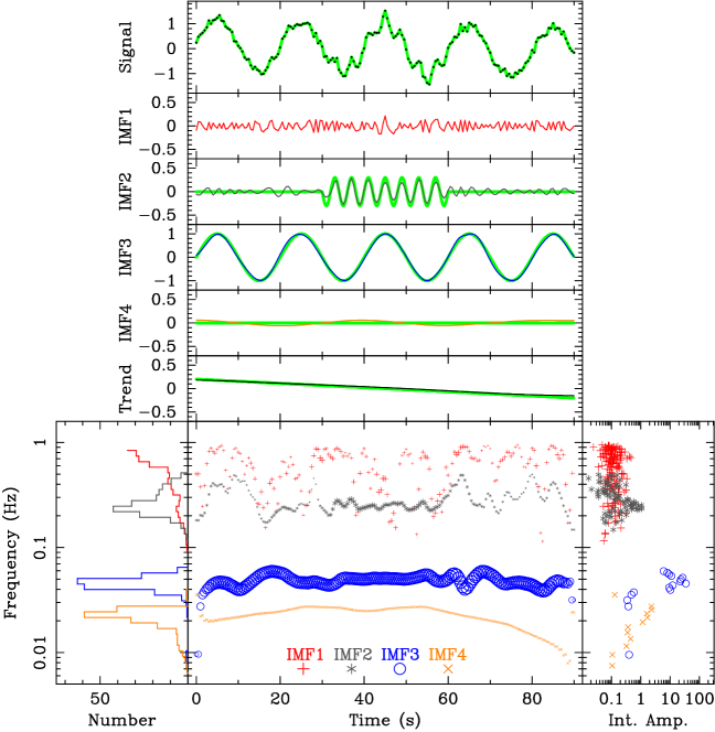
Figure 1: Demonstration of the HHT for a simulated time series. The upper panels show the simulated data and IMFs from the EEMD. The simulated time series are represented by the curve and 300 uniformly sampled data points in the top panel. The signal is originally comprised of four components: a linear term of $0.2-0.4~{}t/90.0$ (the same line in the trend panel), a low frequency oscillation of $1.0\sin(2\pi/20.0~{}t)$ (the curve in the panel for IMF3), a high frequency oscillation of $0.3\sin(2\pi/4.0~{}t)$ appearing between 30 s and 60 s (the curve in the panel for IMF2), and a normally distributed random noise with $\sigma=0.1$. The sampled signal is decomposed by the HHT into four IMFs and the trend, i.e., $\rm Signal=\sum_{i=1}^{4}{IMFi}+Trend$: here IMF1 is the noise, IMF2 the high frequency oscillation, IMF3 the low frequency oscillation, and IMF4 the residual of a small amplitude. The bottom panels are the instantaneous frequencies and amplitudes from the Hilbert transform of the four decomposed IMFs, i.e., each point in a given IMF has a corresponding pair of amplitude and frequency. The bottom middle panel is an amplitude-frequency-time plot. The time and frequency are represented by the horizontal and vertical axes. Each IMF has a dominating frequency interval, as shown by the histogram of instantaneous frequencies in the bottom left panel with the peak indicating the most probable frequency. By integrating the instantaneous amplitudes over time, we obtain the distribution of integrated amplitudes over frequency for each IMF, i.e. the marginal spectrum, as shown in the bottom right panel.

Table 1: Observational parameters for DM variations of 30 pulsars and derived parameters for the trend, noise and annual terms.

No.	PSR name	E-Long.	E-Lat.	Obs. No.	Span	$\sigma_{\rm DMX}$	${\rm dDM}/{\rm d}t$	IAnoise	IFnoise	$\rm\Delta DM_{\rm ann.}$	Phaseann.
(1)	(2)	(3)	(4)	(5)	(6)	(7)	(8)	(9)	(10)	(11)	(12)
1	J0023$+$0923	9.07	$6.31$	50	4.4	0.9	$0.37\pm$0.03	0.4$\pm$0.3	4.8$\pm$2.2	10.7$\pm$2.2	92.4$\pm$15.3
2	J0030$+$0451	8.91	$1.44$	102	10.9	0.9	$-0.06\pm$0.01	1.0$\pm$0.8	5.9$\pm$4.3	7.2$\pm$1.2	88.9$\pm$15.3
3	J0340$+$4130	62.61	$21.33$	56	3.8	1.5	$10.45\pm$0.16	1.3$\pm$0.6	5.1$\pm$2.0	-	-
4	J0613$-$0200	93.80	$-25.41$	121	10.8	0.8	$-1.61\pm$0.07	0.6$\pm$0.3	4.8$\pm$2.0	1.3$\pm$0.2	181.0$\pm$15.3
5	J0645$+$5158	98.06	$28.85$	61	4.5	1.1	$-0.29\pm$0.05	0.6$\pm$0.4	5.3$\pm$2.3	1.7$\pm$0.2	177.5$\pm$16.7
6	J1012$+$5307	133.36	$38.76$	123	11.4	1.5	$1.24\pm$0.01	1.4$\pm$0.9	4.6$\pm$2.5	1.4$\pm$0.5	215.2$\pm$15.4
7	J1024$-$0719	160.73	$-16.04$	82	6.2	1.0	$2.19\pm$0.13	1.3$\pm$0.8	4.8$\pm$2.1	1.5$\pm$0.3	237.3$\pm$15.4
8	J1455$-$3330	231.35	$-16.04$	108	11.4	3.0	$1.44\pm$0.04	3.8$\pm$2.3	4.5$\pm$2.5	4.9$\pm$1.7	317.0$\pm$16.3
9	J1600$-$3053	244.35	$-10.07$	106	8.1	1.0	$0.73\pm$0.32	1.2$\pm$0.6	5.8$\pm$4.3	2.9$\pm$0.4	320.4$\pm$15.3
10	J1614$-$2230	245.79	$-1.26$	91	7.2	1.5	$-0.32\pm$0.04	1.2$\pm$0.8	10.6$\pm$15.3	5.1$\pm$0.7	324.3$\pm$15.1
11	J1640$+$2224	243.99	$44.06$	110	11.1	0.5	$0.75\pm$0.02	0.6$\pm$0.7	6.2$\pm$4.9	-	-
12	J1643$-$1224	251.09	$9.78$	122	11.2	3.1	$-10.73\pm$0.15	4.6$\pm$2.5	6.1$\pm$6.7	5.7$\pm$1.7	232.9$\pm$16.8
13	J1713$+$0747	256.67	$30.70$	209	10.9	0.3	$-0.14\pm$0.01	0.3$\pm$0.2	11.2$\pm$6.6	1.3$\pm$0.1	327.7$\pm$15.2
14	J1738$+$0333	264.09	$26.88$	54	6.1	3.0	$-7.75\pm$0.17	2.6$\pm$1.3	5.1$\pm$2.8	-	-
15	J1741$+$1351	264.36	$37.21$	59	6.4	0.7	$-2.40\pm$0.05	1.1$\pm$0.9	5.0$\pm$2.9	0.6$\pm$0.5	0.6$\pm$17.4
16	J1744$-$1134	266.12	$11.81$	116	11.4	0.7	$-0.17\pm$0.07	1.1$\pm$0.8	4.8$\pm$3.6	1.8$\pm$0.3	349.8$\pm$15.1
17	J1747$-$4036	267.58	$-17.20$	54	3.8	6.0	$-23.37\pm$1.49	11.2$\pm$4.8	5.7$\pm$2.5	-	-
18	J1853$+$1303	286.26	$35.74$	53	4.5	1.0	$0.77\pm$0.05	0.7$\pm$0.4	5.0$\pm$2.7	2.1$\pm$0.4	343.9$\pm$15.4
19	J1857$+$0943	286.86	$32.32$	101	11.0	0.4	$3.01\pm$0.08	0.9$\pm$0.5	4.4$\pm$2.8	2.8$\pm$0.5	329.3$\pm$16.8
20	J1909$-$3744	284.22	$-15.16$	165	11.2	0.5	$-2.08\pm$0.01	0.2$\pm$0.2	3.6$\pm$4.4	1.6$\pm$0.2	8.5$\pm$15.1
21	J1918$-$0642	290.31	$15.35$	117	11.2	1.0	$-2.84\pm$0.11	0.9$\pm$0.5	4.7$\pm$2.5	2.1$\pm$0.4	16.4$\pm$15.4
22	J1923$+$2515	297.98	$46.70$	48	4.3	0.3	$1.13\pm$0.12	1.6$\pm$1.7	4.9$\pm$2.5	-	-
23	J1939$+$2134	301.97	$42.30$	165	11.3	1.0	$-0.10\pm$0.12	0.9$\pm$0.5	7.7$\pm$4.7	2.8$\pm$0.8	220.7$\pm$15.1
24	J1944$+$0907	300.00	$29.89$	53	4.4	1.0	$-8.46\pm$1.12	1.2$\pm$1.1	4.4$\pm$1.7	-	-
25	J2010$-$1323	301.92	$6.49$	88	6.2	0.9	$1.97\pm$0.15	1.7$\pm$1.1	6.7$\pm$10.1	5.4$\pm$0.9	10.3$\pm$15.1
26	J2043$+$1711	318.87	$33.96$	64	4.5	0.4	$0.61\pm$0.05	0.3$\pm$0.2	9.8$\pm$6.1	1.5$\pm$0.2	43.2$\pm$15.2
27	J2145$-$0750	326.02	$5.31$	107	11.3	1.5	$1.19\pm$0.04	2.3$\pm$1.7	7.0$\pm$11.2	3.0$\pm$0.8	58.7$\pm$17.0
28	J2214$+$3000	348.81	$37.71$	53	4.2	3.0	$0.29\pm$0.10	7.9$\pm$5.7	6.1$\pm$3.0	-	-
29	J2302$+$4442	9.78	$45.67$	58	3.8	2.5	$-4.77\pm$0.09	1.6$\pm$0.9	6.5$\pm$2.9	-	-
30	J2317$+$1439	356.13	$17.68$	111	11.0	0.5	$-5.00\pm$0.06	0.3$\pm$0.2	6.2$\pm$5.2	2.2$\pm$0.3	76.6$\pm$15.1
Notes for columns: column (1): index number; column (2): pulsar name; column (3) and (4): ecliptic longitude and latitude, in units of degree; column (5): number of observations for DM; column (6): span for DM data, in units of year; column (7): uncertainty median of DM measurements, in units of $\rm 10^{-4}cm^{-3}pc$; column (8): the average gradient for DM changes, obtained by a linear fitting to the trend curves, in units of $\rm 10^{-4}cm^{-3}pc$ per year; column (9): the median of instantaneous amplitudes for the noise term of DM changes, in units of $\rm 10^{-4}cm^{-3}pc$; column (10): the median of instantaneous frequencies for the noise term of DM changes, in units of $\rm 1/yr$; column (11): the amplitude of annual DM variations, in units of $\rm 10^{-4}cm^{-3}pc$; column (12): the peak phase of annual DM variations, referring to the beginning of a year, in units of degree (1 year = 360∘).

2 The Hilbert Huang Transform

The HHT has been developed to process nonlinear and non-stationary signals (Huang et al., 1998, 1999). It has been used in many research areas already, e.g. in the area of geophysics and meteorology for decomposing the ionospheric scintillation effects from the global navigation satellite system signals (e.g. Sivavaraprasad et al., 2017) or retrieving wind direction from rain-contaminated X-band nautical radar sea surface images (e.g. Liu et al., 2017), in the area of Solar physics for analyzing the Sunspot Numbers (e.g. Gao, 2016), and in the area of astrophysics for analyzing gravitational waves from the late inspiral, merger, and post-merger phases of binary neutron stars coalescence (e.g. Kaneyama et al., 2016). However, it has not heretofore been used for any analysis of real pulsar data.

The HHT consists of “empirical mode decomposition” (EMD) and the well-known Hilbert transform. The EMD can decompose any complicated data set into a finite and often small number of “intrinsic mode functions” (IMFs) without a priori basis unlike Fourier-based methods. These IMFs are generally in agreement with physical signal interpretations, and hence the method can give sharp identifications of embedded structures. These IMFs are then transformed to the Hilbert spectrum to demonstrate the energy-frequency-time distribution of the signal.

To calculate the EMD of a given signal, $x(t)$, its local maxima and minima are firstly identified, and then the envelops for both types of extremes are constructed. A mean curve is calculated by averaging both envelops, which is then subtracted from the signal. This procedure is called “sifting”, and iteratively done many times until the remaining signal meets the following criteria: 1) the number of extremes and the number of zero crossings are equal or differ by one; 2) the mean for the envelops is zero. After this iterative process, the finest component of the signal, i.e. the first intrinsic mode function (IMF1), $c_{1}(t)$, is decomposed, which shows very fast variations depending on the sampling cadence.

After this, the first residual, $r_{1}(t)=x(t)-c_{1}(t)$, is computed, which now serves as the input signal for re-doing the iterative sifting processes to get IMF2, $c_{2}(t)$. Then, the second residual, $r_{2}(t)=r_{1}(t)-c_{2}(t)$, is obtained as the input signal for $c_{3}(t)$, etc. Such a decomposition procedure is iteratively done to get IMF1 to IMF$n$, until the residual, $r_{n}(t)$, becomes monotonic or has only one extremum, which is called the “trend” term. The original signal thus can be expressed as,

$$x(t)=\sum_{j=1}^{n}{c_{j}(t)}+r_{n}(t).$$ (3)

See the upper panels of Figure 1 for illustration of the EMD of a simulated signal.

The EMD has been proved to be very useful in geophysics, solar physics and other scientific fields, as mentioned above. However, it still has some drawbacks. The most serious problem is the mode mixing, i.e. a signal of similar scales and frequencies appears in different IMFs. The Ensemble Empirical Mode Decomposition (EEMD), a noise assisted data analysis method, was later developed by Wu & Huang (2009) to solve the problem, in which the independent white noise realizations are performed and added to the original data to get an ensemble of EMDs. The IMFs of an ensemble of EMDs are then averaged to eliminate the added white noise, by which the mixed modes can be separated.

For each of the decomposed IMFs, the Hilbert transform can be applied to obtain their instantaneous frequencies and amplitudes. The Hilbert transformation of a signal, $x(t)$, can be written as:

$$y(t)=\frac{P}{\pi}\int_{-\infty}^{-\infty}{\frac{x(\tau)}{t-\tau}d\tau}.$$ (4)

Here, $P$ is the Cauchy principal value of the signal integration. The complex signal then reads

$$z(t)=x(t)+iy(t)=a(t)\exp^{i\theta(t)},$$ (5)

and $a(t)$ and $\theta(t)$ represent the instantaneous amplitude and phase. The instantaneous frequency is defined as

$$\omega(t)=\frac{d\theta}{dt}.$$ (6)

Instantaneous frequencies and amplitudes of the IMFs demonstrate the energy-time-frequency distribution for the input signal $x(t)$, as shown in the bottom panels of Figure 1. The EMD or EEMD and Hilbert spectral analysis are combined together to form the Hilbert-Huang Transform (HHT). The open tools of the HHT are available at the web-page.

3 HHT analysis of pulsar DM variations

We apply the HHT method to the temporal variations of pulsar DMs. DM data of 30 pulsars, called “DMX” standing for the offsets from the formal DM values in the ephemerides, are taken from Arzoumanian et al. (2018). These pulsars have been observed for the North American Nanohertz Observatory for Gravitational Waves project, and more than 48 DM measurements over more than 3.8 years are available (see Table 1) for each one. We firstly decompose the DM time series directly by EEMD for the long term “general trend” (not just the trend from the HHT, see below) and the short term “random noise”, and then obtain the annual DM variations by folding the trend- and noise-subtracted data.

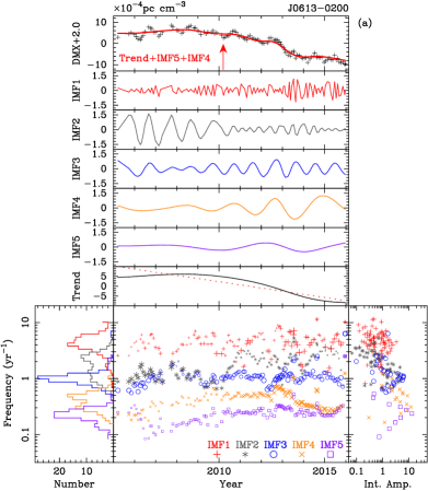
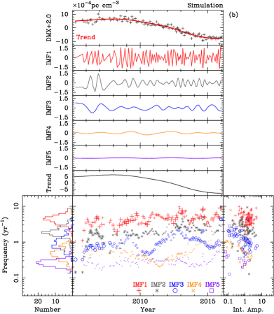
Figure 2: The HHT for DM variations of PSR J0613-0200. (a) The EEMD and Hilbert spectral analysis of observed DM variations are demonstrated in the upper and bottom panels, respectively. In the upper panels, the temporal DM variations (i.e. DMX, in units of $10^{-4}$ pc cm^-3) are represented by “+” in the top panel. The measurements after the epoch indicated by red arrow have a higher observation cadence and used for folding for the annual variation term. The EEMD results, i.e., IMF1 to IMF5 and the trend, are demonstrated in red, grey, blue, orange, purple and black in the panels downward. The trend is fitted by a dotted line to get an average gradient of DM variations as listed in Table 1. The general trend, not just the EEMD trend term, are composited by "Trend+IMF5+IMF4", representing variations with periodicity longer than one year. Instantaneous frequencies and amplitudes of the IMFs for the Hilbert spectrum are shown in the bottom panels. The amplitude-frequency-time plot, histogram for the instantaneous frequencies and the marginal spectrum for each IMF are shown in the middle, left and right panel, respectively, see the keys in Fig. 1. (b) The EEMD and Hilbert spectra of the simulated DM variations, which have the same cadence as real observations of this pulsar and do not show an annual variation term from EEMD.

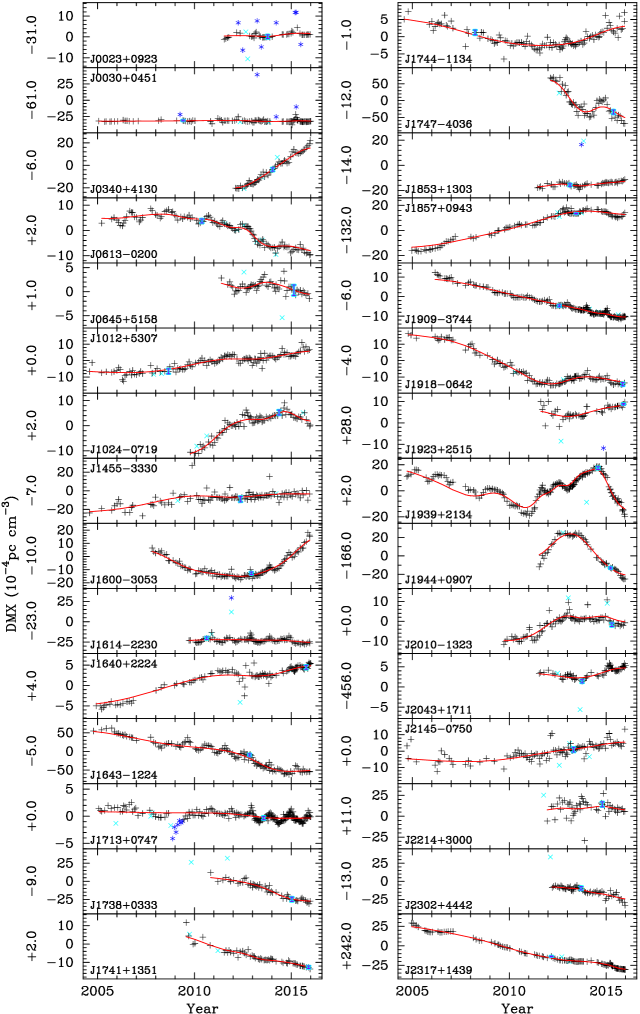
Figure 3: Temporal DM variations of 30 pulsars and the general trends represented by the curves. Normal data are indicated by plus, DM measurements with uncertainties three times larger than their median are indicated by "$\times$” and discarded in the analysis. The data deviating from their neighbors by more than ten times the median variation, as indicated by the asteroids, are also omitted in the HHT analysis, for example, the steep drop and recovery of DM variation for PSR J1713+0747 caused by scattering.

3.1 EEMD for the general trend and noise

DMXs are very small deviations from the formal DM values of pulsars and scaled to the units of $10^{-4}$ pc cm^-3. Through EEMD, DMX time series can be decomposed: DMX = $\sum_{i=1}^{N}$ IMFi + trend. Figure 2 shows an example of the EEMD for IMFs.

It is noticed that each DMX measurement has an uncertainty. The uncertainties for data obtained in early years are much larger than those in the recent years because of lower sensitivity of the old observing systems with limited observing bandwidth. Since the uncertainties are not concerned in EEMD, we have to “clean” the DMX data before the EEMD process. We first omit those data with a very large uncertainty (three times larger than the median uncertainty), which are often deviated from the general trend (see Arzoumanian et al., 2015). Some data are occasionally very (ten times larger than the median derivation) deviated from their adjacent measurements as caused by the very sharp annual DM variations (e.g. J0023+0923) or the extreme scattering event (e.g. PSR J1713+0747) (Arzoumanian et al., 2015; Coles et al., 2015; Lentati et al., 2016), which are also not the proper tracers for the trend. If these data points are otherwise included, the HHT analysis will introduce a number of oscillations with various amplitudes and frequencies to the IMFs at their instants.

HHT analysis of the “cleaned” DMX data gives IMF1 to IMF5 and the trend, as shown for the DM time series for PSR J0613$-$0200 in Figure 2. The “noise” term is IMF1 as seen in the upper panels of Figure 2(a), which represents the finest structure of DM variation with a time scale depending on the observational cadence. The Hilbert transform of IMF1 gives its instantaneous frequencies and amplitudes, as shown by red dots in the bottom middle panel of Figure 2(a). The median values of instantaneous amplitudes and frequencies as well as their standard deviations can be found for this random noise component of DM variations, as listed in columns (9) and (10) in Table 1. IMF3 and IMF2 are annual and semi-annual variations, which will be analyzed in the next section.

The EEMD trend term for DM variations of PSR J0613$-$0200 is not linear but can still be fitted approximately with a line to get the rough rate of DM changes, i.e. ${\rm d}{\rm DM}/{\rm d}t$, as also listed in column (8) of Table 1. The general trend term for DM variations of PSR J0613$-$0200, however, is not just the EEMD trend term, but is composited by "Trend+IMF5+IMF4" which shows long-term variations with time-scales longer than one year, as indicated the line in the top panel.

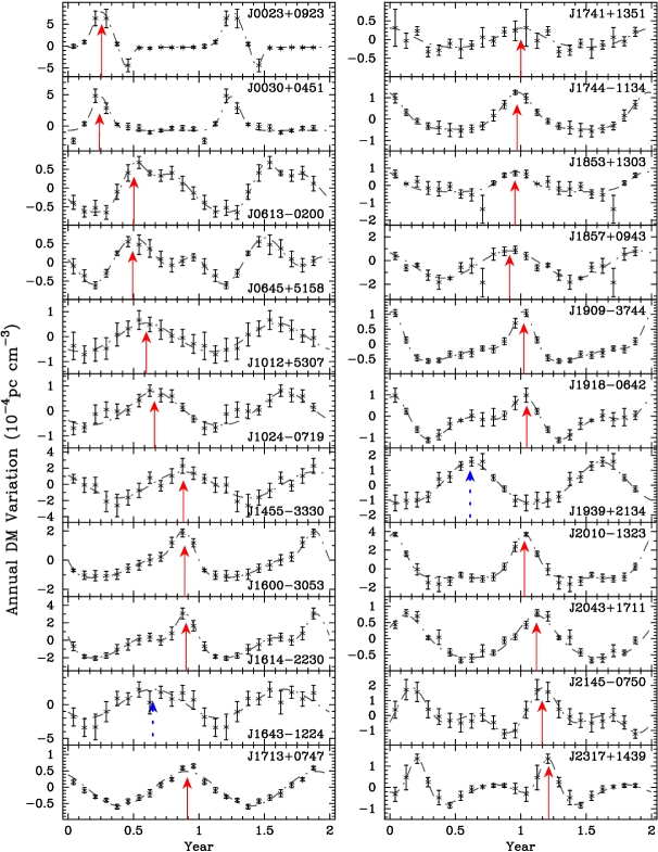
Figure 4: Annual DM variations of 22 pulsars, obtained by folding data obtained in recent years with one year period (referring to the beginning of a year) after the “general trend” and noise terms are subtracted (see plots for DM variations in Figure 6). Two cycles are plotted for clarity. The fitted von Mises (circular normal) curves are plotted by dash-dotted lines, and the peak phases of annual variations are indicated by arrows. Two pulsars, PSRs J1643$-$1224 and J1939+2134, have extraordinary peak phases as indicated by dashed arrows.

To demonstrate the effectiveness of the HHT in decomposing DM variations, we simulate a DM time series by using the trend term of Figure 2(a) plus the white noises. The simulated data in Figure 2(b) have the same cadence as the real observations for PSR J0613$-$0200. The HHT decomposes the simulated data into five IMFs and trend term. Though each IMF has a dominating frequency range, but is not sharply peaked at any given frequency (e.g. one year^-1). The marginal spectra have comparable power among these IMFs, rather than a significant power excess for a given IMF. It is also noticed that the phases for the peaks of a given IMF (e.g. IMF2 and IMF3) vary a lot, rather than being fixed at a given phase over years. In other words, these IMFs of simulated data do not show any significant periodic signal, which demonstrate that HHT does not artificially introduce any regular annual signals in the DM time series.

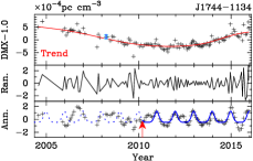
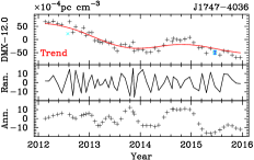
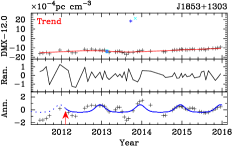
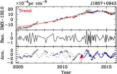
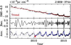
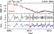
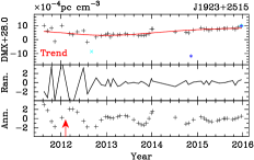
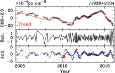
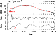
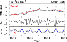
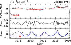
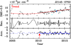
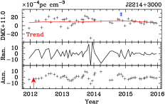
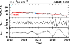
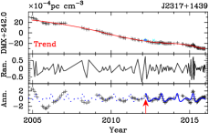
Figure 6: Continued–

As shown in Appendix A, we have also decomposed the noise terms and the general trends for 30 pulsars (see Figure 6). The general trends have also been plotted together with data in Figure 3.

3.2 Annual variations from folding DMX data

There is no doubt that annual variations exist for pulsar DMs, which have been shown by clear frequency peaks for IMF2 and IMF3 of PSR J0613$-$0200 in Figure 2 (a). Observations with higher cadence since the year of about 2010 (see Figure 6) exhibit clear semi-annual and annual variations.

Annual variations do not have to follow the sinusoidal curve (Lam et al., 2016). They can have frequencies of annual and semi-annual and other forms as shown by Figure 2 (a). Such an annual variation can be obtained by adding IMF2 and IMF3. The most effective approach to get the annual term is folding the DMX curves with an one-year period, after the general trend and noise terms are subtracted from the original data. Data of the recent observations after the epoches indicated by the arrows in Figure 2(a) and Figure 6 are folded into 12 bins, corresponding to 12 months a year. DMX data in each bin are weighting averaged according to the measurement uncertainty. Among the 30 pulsars, 7 pulsars show complicated structures in the trend- and noise-subtracted data, and no annual variations can be identified within short data spans. The other one, PSR J1640+2224, shows a complicated feature (see Figure 6). The resulting annual curves for the remaining 22 pulsars are displayed in Figure 6 and Figure 4.

As shown in Figure 3, data deviating from the adjacent measurements by more than ten times the median derivation were omitted for the trend analysis for 5 pulsars. Most of these “cleaned” data are around the peaks for annual variations (see Figure 6 for PSRs J0023+0923, J0030+0451 and J1614$-$2230). Outlying data indicated by asteroids near the curve peak are taken back to form the annual variation curves, if they do not significantly differ from data in other peaks. Though near each peak only one measurement is available, the repeatedly outlying data near the peak of annual variations for PSRs J0023+0923 and J0030+0451 indicate that the real peak should be much more sharp than we see from merely one measurement each. For PSRs J1614$-$2230, J1853+1303 and J1923+2515, only one data point is abnormal near the peak, which is not taken back because no recurrence has been observed for confirmation. The data points for extreme scattering event of PSR J1713+0747 are certainly not included to fold for the annual curve.

To quantitatively describe the annual variations, we fit the von Mises functions (i.e. the circular normal function) to the folded annual curves. For the curves for PSRs J0023+0923, J0613$-$0200, J0645+5158, J1600$-$3053, J1614$-$2230, J1909$-$3744, J1918$-$0642, J2145$-$0750, and J2317+1439, a single von Mises function is not enough and two von Mises functions are employed for the fitting. The peak phases are referenced to the beginning of a year, and can be so-obtained during the fitting as indicated by the arrows in Figure 4. The amplitudes of annual variations are simply taken as the difference between the maximum and minimum of the folded data. These values are listed in columns (11) and (10) in Table 1, respectively.

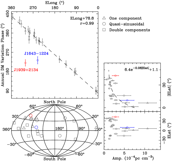
Figure 5: Distribution of 22 pulsars with respect to the ecliptic frame (bottom left panel). The phases and amplitudes of annual variations are related to the ecliptic longitude and latitude in the upper and right panels. Three kinds of annual variations, one component, quasi-sinusoidal and double components features, are represented by triangle, circle and rectangle points, respectively. Right panels: Amplitudes of annual variations are related to the ecliptic latitude or their absolute values (upper panel). Top panel: Phases of annual variations are well correlated to the ecliptic longitude, with a correlation factor of $r=0.99$. The best fittings for the dependencies are indicated by the dashed lines. Two exceptions (PSRs J1643$-$1224 and J1939+2134) are marked.

4 Discussions

We have decomposed the temporal DM variations of 30 pulsars into general trends and small-amplitude random fast DM changes by using the EEMD of the HHT, and then obtained the annual variation curves of 22 pulsars by folding the trend- and noise-subtracted DMX data.

4.1 The trend and noise

The general trends exhibit monotonic increasing, decreasing, or complicated variations (see Figure 3 for the 30 pulsars). Clear monotonic DM decreasement has been observed for PSRs J1614$-$2230, J1643$-$1224, J1713+0747, J1738+0333, J1741+1351, 1909$-$3744, J2302+4442 and J2317+1439, clear monotonic DM increasement for PSRs J0340+4130, J1012+5307 and J1455$-$3330, and quadratic variations for PSRs J1600$-$3053 and J1944+0907. The ${\rm dDM}/{\rm d}t$ values in Table 1 obtained by the simple linear fitting to the EEMD trend term can only roughly reflect the averaged DM gradient, and listed there for comparison with those in Jones et al. (2017) from the 9 year data-set of Arzoumanian et al. (2015). PSRs J0340+4130, J1643$-$1224, J1747$-$4036 and J1944+0907 have the largest gradients for DM variations, more than $8\times 10^{-4}{\rm cm}^{-3}{\rm pc}$ per year. As discussed in Lam et al. (2016), the relative line-of-sight motion between the Earth and pulsar can produce monotonically varying DM if density gradients of interstellar medium are not taken into account. Otherwise, plasma wedges can also cause linear trends (Backer et al., 1993). In most cases, the DM variations exhibit much complicated trends. For example, PSR J1939+2134 has a DM decreased before 2011 and increased afterwards to 2014, after which it decreases again. PSR J1747$-$4036 demonstrates similar variation features, but with much shorter time scale. They may be caused by the transverse motion of a large interstellar cloud into or out of the line of our sight. Moreover, ionized bow shocks and stochastic process of the interstellar medium with a red power spectrum may also cause non-monotonic trends for the DM variations (Lam et al., 2016).

By performing EEMD on the DM time series, we got the random terms of DM variations, as shown by IMF1 in Figure 2 (a) for PSR J0613$-$0200 and the middle panel in each plot of Figure 6 for other pulsars. The medians for the instantaneous frequencies of IMF1s range from 3.6 to 10.6 per year as listed in Table 1, which in fact reflect only the main cadence of observations. This “noise” part of the observed DMs comes from random contributions from interstellar medium, interplanetary medium and ionosphere, but it should have turbulence at different physical and hence time scales (Armstrong et al., 1995). The small-scale turbulence in interstellar medium can cause much faster DM variations, such as the extreme scattering-like variation of PSR J1713+0747 around 2009. For the Kolmogorov turbulence, it was predicted that the power spectrum of the DM variations has a spectral index of 8/3 (Lam et al., 2016). More frequent observations in future can reveal better the turbulence at different scales in the interstellar medium, interplanetary medium and ionosphere. In addition, EEMD also demonstrates low frequency variations with periodicity longer than one year, which may be mixed with the trend term. Though HHT can decompose DM variations into a number of components with different time scales, it is very premature to use them to interpret the detailed structures of interstellar medium.

4.2 Annual DM variations

Annual pulsar DM variation caused by the variable interplanetary medium and Solar wind has been known for a long time (e.g. You et al., 2007a). Keith et al. (2013) found an annual periodicity for PSRs J0613$-$0200, J1045$-$4509, J1643$-$1224 and J1939$+$2134 from spectral analysis of DM variations obtained by the Parkes Pulsar Timing Array project. Lam et al. (2016) obtained the annual variation of PSR J1909$-$3744 by subtracting a linear trend from the DM measurements. Jones et al. (2017) detected annual DM variations for an ensemble of pulsars from the 9-year data set of Arzoumanian et al. (2015) by decomposing the time series with annual triangle functions and Lomb-Scargle periodogram analysis.

We obtained the annual variation curves for 22 pulsars (see Figure 4 and Figure 6) especially by using the data of high quality recent observations from Arzoumanian et al. (2018). Compared with previous analyses, annual variation curves of 9 pulsars (PSRs J0023+0923, J1012+5307, J1024-0719, J1455$-$3330, J1600-3053, J1713+0747, J1741+1351, J1853+1303, and J2145-0750) are obtained here for the first time, and the curves for other pulsars are significantly improved.

As seen from Figure 4, annual variations exhibit three kinds of features. A simple quasi-sinusoidal variation has been obtained for PSRs J1012+5307, J1024$-$0719, J1455$-$3330, J1643$-$1224, J1741+1351, J1857+0943 and J1939+2134. These pulsars are generally away from the ecliptic plane (see Figure 5), and the quasi-sinusoidal variations can be understood by the trajectory of Earth in the interplanetary medium (Keith et al., 2013). One peak component of variations can be seen for PSRs J0023+0923, J0030+0451, J1713+0747, J1744$-$1134, J1853+1303, J2010$-$1323 and J2043+1711. These pulsars are located at low ecliptic latitudes and seriously affected by electron density contributed by the solar wind. The strange DM “absorption” after the peak for PSR J0023+0923 has been detected in three years (see Figure 6), and therefore it is confirmed but not explainable. The “absorption” before the peak of PSR J0030+0451 is still to be confirmed. Double peaks of variations can be seen for PSRs J0613$-$0200, J0645+5158, J1600$-$3053, J1614$-$2230, J1909$-$3744, J1918$-$0642, J2145$-$0750, and J2317$+$1439, which may result from the coupled effects of the ionosphere together with the interplanetary medium.

With the annual variations of a large sample of 22 pulsars, we can check the correlations of both the amplitudes and phases of annual variations with the ecliptic coordinates, as shown in Figure 5. In general the higher-density slow wind appears at lower ecliptic latitude and the lower-density fast wind at higher latitude. Because the electron density generally scales with distance $r$ from the Sun by following $r^{-2}$, the amplitudes of annual variations should also vary with ecliptic latitude. The correlation of annual variations with solar position angle has been analyzed for some individual pulsar previously, for example a strong correlation was found for PSRs J0030+0451 and J1614-2230 and a moderate correlation for PSR J2010-1323 (Jones et al., 2017). The DM variations of PSR J1909$-$3744 have been analyzed by Lam et al. (2016) with modeling the annual variations by the solar wind as well as ionosphere and heliosphere. We found from our new curves that pulsars closer to the ecliptic plane tend to have larger amplitudes for annual variations, which can be roughly described by an exponential function. The peak phases of annual variations are well correlated with the ecliptic longitude, with a correlation coefficient $r=0.99$, if two exceptions (PSRs J1643$-$1224 and J1939+2134) are not considered.

Apparent annual variations for PSRs J1643$-$1224 and J1939+2134 are very different. Their amplitudes are somehow larger than the expected values from the fitted exponential function curve. Their peak phases are very exceptional, which indicate that annual variations of both pulsars might not only result from the solar wind. It should be noted that the amplitude for annual variation of PSR J1643$-$1224 is very large (up to $5.7\times 10^{-4}{\rm cm}^{-3}{\rm pc~{}}$) and the trend curve for PSR J1939+2134 is the most complicated. These “annual” variations may be caused by quasi-periodically crossing of the interstellar cloud by sight lines, so that their phases can be arbitrary (Lam et al., 2016). By jointly investigating temporal variations in DM and scattering in the ionized interstellar medium through the Bayesian approach, Lentati et al. (2017) also suggested that the scattering variation of interstellar clouds is the most possible cause for the period apparent DM variation observed in PSR J1643$-$1224.

5 Conclusions

We decomposed the temporal DM variations of 30 pulsars into general trends, random components and annual variations by employing the HHT method. We found that HHT can extract the general trends from data, which represent the largest structures of DM variations resulting from the irregularly distributed interstellar medium. The random DM components heavily depend on the cadence of observations. Annual variations of 22 pulsars can be extracted from the trend- and noise-subtracted DM data, which exhibit quasi-sinusoidal, one component and double components features. The amplitudes and phases of annual variations are well related to ecliptic latitude and longitude, respectively, whose origins are attributed to the DM variations from solar wind and interplanetary medium. The exceptions are probably caused by the interstellar medium.

In future, observations with higher cadence can help us to understand the turbulent feature of the interstellar medium. Long-term observations can be used to reveal the long-term variations due to the interstellar refractive scattering or the annual variations caused by the solar wind and interplanetary medium. Therefore, sensitive wide-band observations of more pulsars with higher cadence in longer time spans are very important, which can not only show the high precision DM variations in great details, but also reveal the details of the interplanetary and interstellar medium. In addition, the HHT can also be implemented into the Bayesian pulsar timing algorithms to check if the timing noises have variations on different temporal scales.

Appendix A Plots for the trend, random, and annual variations for pulsar DMs

We present the temporal DM series and the general trends, random fast variations and annual variation components for all 30 pulsars.

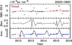
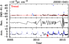
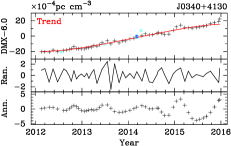
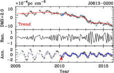
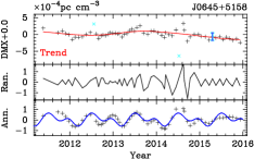
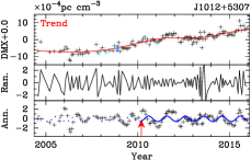
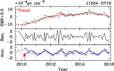
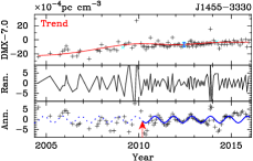
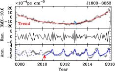
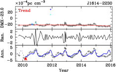
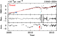
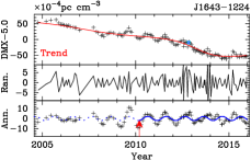
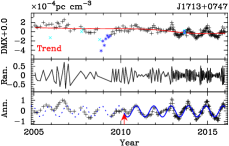
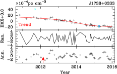
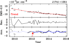
Figure 6: For each pulsar, the original DMX data are shown in the top panel together with the “general trend”. The data are plotted in different symbols as in Figure 3: normal data by “+”; measurements with uncertainties three times larger than the median uncertainty are indicated by “$\times$”; the data deviating from their neighbors by more than ten times the median deviation are indicated by the asteroids. The middle panel is plotted for the random fluctuations obtained as IMF1 by the EEMD, with simply connected lines. The data with “general trend” and noise subtracted are then plotted in the bottom panel, with the annual variation curves plotted in the solid line after the epoch indicated by the arrow after which data were used for folding for the annual curves. The curves are extended to early data by the dotted line. Outlying data indicated by asteroids near the curve peaks are taken back to form the annual variation curves, if they do not differ significantly from the data at other peaks.

References

- Armstrong et al. (1995) Armstrong J. W., Rickett B. J., Spangler S. R., 1995, ApJ, 443, 209
- Arzoumanian et al. (2015) Arzoumanian Z., Brazier A., Burke-Spolaor S., et. al. 2015, ApJ, 813, 65
- Arzoumanian et al. (2018) Arzoumanian Z., Brazier A., Burke-Spolaor S., et. al. 2018, ApJS, 235, 37
- Backer et al. (1993) Backer D. C., Hama S., van Hook S., Foster R. S., 1993, ApJ, 404, 636
- Caballero et al. (2016) Caballero R. N., et al., 2016, MNRAS, 457, 4421
- Coles et al. (2015) Coles W. A., Kerr M., Shannon R. M., et. al. 2015, ApJ, 808, 113
- Demorest et al. (2013) Demorest P. B., et al., 2013, ApJ, 762, 94
- Desvignes et al. (2016) Desvignes G., et al., 2016, MNRAS, 458, 3341
- Gao (2016) Gao P. X., 2016, ApJ, 830, 140
- Huang & Roussel-Dupré (2006) Huang Z., Roussel-Dupré R., 2006, Radio Science, 41, RS6004
- Huang et al. (1998) Huang N. E., et al., 1998, RSPSA, 454, 903
- Huang et al. (1999) Huang N. E., Shen Z., Long S. R., 1999, ARFM, 31, 417
- Jones et al. (2017) Jones M. L., McLaughlin M. A., Lam M. T., et. al. 2017, ApJ, 841, 125
- Kaneyama et al. (2016) Kaneyama M., Oohara K.-i., Takahashi H., Sekiguchi Y., Tagoshi H., Shibata M., 2016, Phys. Rev. D, 93, 123010
- Keith et al. (2013) Keith M. J., Coles W., Shannon R. M., et. al. 2013, MNRAS, 429, 2161
- Lam et al. (2016) Lam M. T., Cordes J. M., Chatterjee S., Jones M. L., McLaughlin M. A., Armstrong J. W., 2016, ApJ, 821, 66
- Lee et al. (2014) Lee K. J., et al., 2014, MNRAS, 441, 2831
- Lentati et al. (2016) Lentati L., Shannon R. M., Coles W. A., et. al. 2016, MNRAS, 458, 2161
- Lentati et al. (2017) Lentati L., Kerr M., Dai S., Shannon R. M., Hobbs G., Osłowski S., 2017, MNRAS, 468, 1474
- Liu et al. (2017) Liu X., Huang W., Gill E. W., 2017, IEEE Transactions on Geoscience and Remote Sensing, 55, 1833
- Lyne et al. (1988) Lyne A. G., Pritchard R. S., Smith F. G., 1988, MNRAS, 233, 667
- Opher et al. (2015) Opher M., Drake J. F., Zieger B., Gombosi T. I., 2015, ApJL, 800, L28
- Petroff et al. (2013) Petroff E., Keith M. J., Johnston S., van Straten W., Shannon R. M., 2013, MNRAS, 435, 1610
- Reardon et al. (2016) Reardon D. J., Hobbs G., Coles W., et. al. 2016, MNRAS, 455, 1751
- Sivavaraprasad et al. (2017) Sivavaraprasad G., Sree Padmaja R., Venkata Ratnam D., 2017, IEEE Geoscience and Remote Sensing Letters, 14, 389
- Wu & Huang (2009) Wu Z. H., Huang N. E., 2009, Adv. Adapt. Data Anal., 01, 1
- You et al. (2007a) You X. P., Hobbs G., Coles W. A., et. al. 2007a, MNRAS, 378, 493
- You et al. (2007b) You X. P., Hobbs G. B., Coles W. A., Manchester R. N., Han J. L., 2007b, ApJ, 671, 907