Molecular Clouds associated with the Type Ia SNR N103B in the Large Magellanic Cloud

Abstract

N103B is a Type Ia supernova remnant (SNR) in the Large Magellanic Cloud (LMC). We carried out new ¹²CO($J$ = 3–2) and ¹²CO($J$ = 1–0) observations using ASTE and ALMA. We have confirmed the existence of a giant molecular cloud (GMC) at $V_{\mathrm{LSR}}$ $\sim$245 km s^-1 towards the southeast of the SNR using ASTE ¹²CO($J$ = 3–2) data at an angular resolution of $\sim$25$\arcsec$ ($\sim$6 pc in the LMC). Using the ALMA ¹²CO($J$ = 1–0) data, we have spatially resolved CO clouds along the southeastern edge of the SNR with an angular resolution of $\sim$1.8$\arcsec$ ($\sim$0.4 pc in the LMC). The molecular clouds show an expanding gas motion in the position–velocity diagram with an expansion velocity of $\sim 5$ km s^-1. The spatial extent of the expanding shell is roughly similar to that of the SNR. We also find tiny molecular clumps in the directions of optical nebula knots. We present a possible scenario that N103B exploded in the wind-bubble formed by the accretion winds from the progenitor system, and is now interacting with the dense gas wall. This is consistent with a single-degenerate scenario.

1 Introduction

Identifying the progenitor system of Type Ia supernovae is a long-standing problem of modern astrophysics, especially in light of their use as standard candles in cosmology (e.g., Perlmutter et al., 1999). At present, two theoretical scenarios have been proposed: A single-degenerate (SD) scenario in which a white dwarf has accreted materials from a non-degenerate companion—a red giant, main-sequence star, or a helium star—until the white dwarf mass gets close to the Chandrasekhar limit $\sim$1.4 $M_{\sun}$ (Whelan & Iben, 1973; Nomoto, 1982; Iben & Tutukov, 1984; Paczynski, 1985), and a double-degenerate (DD) scenario represents the merger of two white dwarfs (Nomoto, 1982; Webbink, 1984).

To distinguish these scenarios, The identification of the companion star and the associated dense circumstellar medium (CSM) is thought to be essential. For the SD scenario, the non-degenerate companion can survive after the explosion of the primary white dwarf (e.g., Kasen, 2010), and binary interactions may produce the dense CSM whose chemical composition is modified by the mass loss from the progenitor system (Hachisu et al., 2008). For the DD scenario, no companion star or dense CSM are expected. Pioneering studies have succeeded in finding the ionized CSM in Kepler’s supernova remnant (SNR) (Douvion et al., 2001; Blair et al., 2007; Williams et al., 2012). The CSM in Kepler’s SNR shows N overabundance, which would be originated by CNO-processed medium from the progenitor system, providing a further support for the SD origin (Katsuda et al., 2015).

Investigating the interstellar neutral gas around Type Ia SNRs has received attention as an alternative approach to understand the nature of progenitor systems Zhou et al. (2016) discovered an expanding bubble surrounding Tycho’s SNR based on the CO data obtained with the IRAM 30 m telescope. The expanding velocity of the bubble was found to be $\sim$4.5 km s^-1 and has a mass of $\sim$220 $M_{\sun}$. Enhanced intensity ratio of ¹²CO $J$ = 2–1 / 1–0 and possible line broadening were also found at the northeastern rim of the SNR. The authors concluded that the bubble was driven by the accretion wind with the velocity of a few hundreds km s^-1, suggesting the SD scenario as the progenitor system of Tycho’s SNR. Subsequently, Chen et al. (2017) found double shell-like structures of CO clouds around Tycho’s SNR. The large CO cavity—a size of 13 pc $\times$ 27 pc—is partially connected with the small CO cavity with a size of $\sim$9 pc, both of which are expanding at a velocity of $\sim 3$–4 km s^-1. The total kinematic energy of CO cavities is consistent with the prediction of the accretion wind model (e.g., Hachisu et al., 1996, 1999a, 1999b). The authors therefore concluded that the large cavity cloud be also formed by the accretion winds from the SD progenitor system of the SNR. To better understand the SD scenario, we need more samples of the Type Ia SNRs associated with the interstellar neutral gas.

N103B (also known as SNR 0509$-$68.7) is one of the youngest Type Ia SNRs in the Large Magellanic Cloud (LMC). The light echo observations estimated the age to be 380–860 yr (Rest et al., 2005). The angular size of N103B is $27^{\prime\prime}\times 29^{\prime\prime}$ corresponding the diameter $\sim$6.8 pc at the LMC distance of 50 kpc (e.g., Maggi et al., 2016; Bozzetto et al., 2017). The Chandra X-ray image (Figure 1a) unveils the bright western-half comprising a series of dense knots and diffuse emission (Lewis et al., 2003). Studies of the X-ray spectroscopy show the large mass of Fe ($\sim$0.34 $M_{\sun}$) and the lack of a region of O-rich ejecta, indicating a Type Ia origin for the SNR (Hughes et al., 1995; Lewis et al., 2003). The presence of highly-ionized Fe suggests the strong interaction between the supernova ejecta and the dense CSM (Yamaguchi et al., 2014). In fact, recent optical and infrared photometric/spectroscopic observations identified the ionized CSM with a density of $\sim$500–5000 cm^-3 and a possible candidate for a surviving main-sequence companion near the center of the SNR, suggesting a likely candidate for the SD origin (Li et al., 2017; Ghavamian et al., 2017). The SD scenario is also supported by measurements of the Ca/S mass ratios by X-ray spectroscopic analysis (Martínez-Rodríguez et al., 2017).

In contrast, detailed studies of the interstellar neutral gas of N103B have not yet been reported. Sano et al. (2017a, 2018) revealed a giant molecular cloud (GMC) in the direction of the SNR N103B using the Mopra 22-m radio telescope. The authors estimated the total mass of GMC to be $\sim$$10^{6}$ $M_{\sun}$, which is significantly higher than the masses of GMCs associated with the LMC SNRs N132D and N49, and the LMC superbubble 30 Doradus C (Banas et al., 1997; Sano et al., 2015, 2017b; Yamane et al., 2018). Despite the promising candidate for the site of shock-cloud interaction, the authors could not resolve the spatial distribution of molecular clouds likely associated with the SNR N103B due to the limited angular resolution of Mopra ($\sim$45^′′ corresponding to $\sim$11 pc in the LMC).

In the present paper, we report new millimeter/submillimeter wavelength observations using ¹²CO($J$ = 1–0, 3–2) emission lines with the Atacama Large Millimeter/submillimeter Array (ALMA) and the Atacama Submillimeter Telescope Experiment (ASTE). Because of the high angular resolution of $\sim$1.8^′′ and $\sim$25^′′ ($\sim$0.4 pc and $\sim$6 pc in the LMC), we can spatially resolve the GMC into individual molecular clouds. Section 2 gives observations and data reductions of CO, Hi, and X-rays. Subsection 3.1 overviews the large-scale Distribution of the X-rays, CO, and Hi; subsections 3.2 and 3.3 present a detailed CO distribution with ALMA. Discussion and conclusions are given in Sections 4 and 5, respectively. In a subsequent paper (Alsaberi et al. 2018 in preparation), we will examine radio continuum component of the N103B with special emphasis on its expansion, polarization and spectral energy distribution.

Table 1: Summary of $Chandra$ archive data

Observation ID	$\alpha_{\mathrm{J2000}}$	$\delta_{\mathrm{J2000}}$	Start Date	Exposure	Roll Angle
	(h m s)	($\arcdeg$ $\arcmin$ $\arcsec$)	(yyyy-mm-dd hh:mm:ss)	(ks)	($\arcdeg$)
00125	05 08 59.00	$-68$ 43 30.00	1999-12-04 12:26:57	36.7	0$+71$
03810	05 08 44.00	$-68$ 45 36.00	2003-02-07 01:29:46	29.7	$-152$
18018	05 08 59.00	$-68$ 43 34.00	2017-03-20 18:12:45	39.5	0$+47$
20042	05 08 59.00	$-68$ 43 34.00	2017-03-24 18:59:37	19.8	0$+39$
19921	05 08 59.00	$-68$ 43 34.00	2017-04-10 22:26:08	16.8	0$+19$
20058	05 08 59.00	$-68$ 43 34.00	2017-04-14 13:57:32	43.8	0$+20$
18020	05 08 59.00	$-68$ 43 34.00	2017-04-17 21:23:32	27.2	0$+25$
19923	05 08 59.00	$-68$ 43 34.00	2017-04-26 19:06:00	58.3	0$+26$
20067	05 08 59.00	$-68$ 43 34.00	2017-05-04 18:49:53	29.7	0$-20$
20053	05 08 59.00	$-68$ 43 34.00	2017-05-22 11:42:30	11.2	0$-61$
18019	05 08 59.00	$-68$ 43 34.00	2017-05-23 19:08:22	59.3	0$-37$
19922	05 08 59.00	$-68$ 43 34.00	2017-05-30 01:23:59	41.4	0$-48$
20085	05 08 59.00	$-68$ 43 34.00	2017-05-31 04:07:23	14.9	0$-54$
20074	05 08 59.00	$-68$ 43 34.00	2017-06-01 19:08:17	31.2	0$-55$

Note. — All exposure times represent the net available times alter several filtering procedures are applied in the data reduction processes.

2 Observations and Data Reductions

2.1 CO

Observations of ¹²CO($J$ = 3–2) line emission at 0.87 mm wavelength were carried out in 16–24 November 2015 using ASTE (Ezawa et al., 2004). We used the on-the-fly (OTF) mapping mode with Nyquist sampling. The map size is $2^{\prime}\times 2^{\prime}$ rectangular region with a center position at ($\alpha_{\mathrm{J2000}}$, $\delta_{\mathrm{J2000}}$) $\sim$ ($05^{\mathrm{h}}08^{\mathrm{m}}59^{\mathrm{s}}$, $-68\arcdeg 43\arcmin 36\arcsec$). The side-band-separating mixer receiver “DASH 345” receiver was used for a front end. The back end was “MAC” digital FX spectrometer (Sorai et al., 2000) with 1024 channels with a bandwidth of 128 MHz, corresponding to the velocity coverage of $\sim$111 km s^-1 and the velocity resolution of $\sim$0.11 km s^-1. The typical system temperature was $\sim$300–600 K in the single-side-band (SSB), including the atmosphere. We smoothed the data with a two-dimensional Gaussian function of $11^{\prime\prime}$. The final beam size is $\sim$25^′′ (FWHM). The pointing accuracy was checked every half-hour to satisfy an offset within $2^{\prime\prime}$. We also observed N159W [($\alpha_{\mathrm{J2000}}$, $\delta_{\mathrm{J2000}}$) $\sim$ ($05^{\mathrm{h}}40^{\mathrm{m}}3\fs 7$, $-68\arcdeg 47\arcmin 00\arcsec$)] (Minamidani et al., 2011) for the absolute intensity calibration, and then we estimated the main beam efficiency of $\sim$0.55. The final data has a noise fluctuation of $\sim$0.11 K at the velocity resolution of $\sim$0.4 km s^-1.

Observations of ¹²CO($J$ = 1–0) line emission at 2.6 mm wavelength were conducted at 31th January and 27th August 2016 using ALMA Band 3 (84–119 GHz) as a Cycle 3 filler project $\#$2015.1.01130.S (PI: Kosuke Fujii). We used the mosaic mapping mode of a $100^{\prime\prime}\times 100^{\prime\prime}$ rectangular region with a center position at ($\alpha_{\mathrm{J2000}}$, $\delta_{\mathrm{J2000}}$) $\sim$ ($05^{\mathrm{h}}08^{\mathrm{m}}59^{\mathrm{s}}$, $-68\arcdeg 43\arcmin 36\arcsec$). The observations were carried out using 38 antennas for 12 m array. The baseline ranges are from 13.7 to 1551.1 m, corresponding to the u-v coverage form 4.6 to 596.0 $k\lambda$. The correlator was set to have a bandwidth of 58.59 MHz, representing the velocity coverage of 152.5 km s^-1. The calibration used three quasars: J0635$-$7516 for the complex gain calibrator, J0519$-$4546 for the flux calibrator, and J0529$-$7245 for the phase calibrator. These calibrations and data reduction were made by the Common Astronomy Software Application (CASA; McMullin et al., 2007) package version 5.1.0. We used the natural weighting and the multiscale CLEAN algorithm (Cornwell, 2008) implemented in the CASA package. The final beam size is $1.92^{\prime\prime}\times 1.73^{\prime\prime}$ with a position angle of $66\fdg 7$, corresponding to the spatial resolution of $\sim$0.44 pc at the LMC distance of 50 kpc. Typical noise fluctuation is $\sim$0.95 K at 0.4 km s^-1 velocity resolution. To estimate the missing flux, we compared the integrated intensity of the Mopra single-dish data (Wong et al., 2011, 2017; Sano et al., 2017a, 2018) with the ALMA CO data that smoothed to match the FWHM of the single-dish data ($\sim$45^′′). Since the total integrated intensity of ALMA data is $\sim$10$\%$ smaller than that of the single-dish data, the missing flux is considered to be negligible.

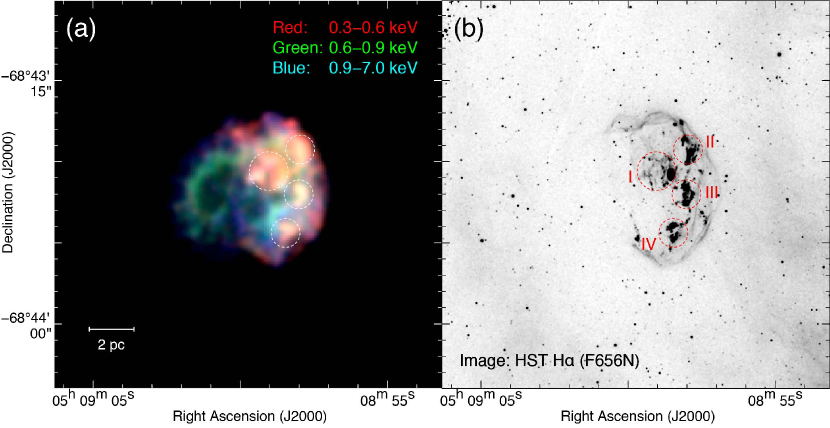
Figure 1: (a) RGB image of X-rays obtained with Chandra (Lewis et al., 2003). The red, green, and blue represent the energy bands, 0.3–0.6 keV, 0.6–0.9 keV, and 0.9–7.0 keV, respectively. (b) H$\alpha$ image using Hubble Space Telescope (HST) with the FW656N filter (Li et al., 2017). Dashed circles indicate the optical nebular knots (I), (II), (III), and (IV) as defined by (Li et al., 2017). We also annotate the dashed circles in Figure 1a.

2.2 Hi

We also used archival Hi 21 cm line data published by Kim et al. (2003). The data were obtained using the Australia Telescope Compact Array (ATCA) and combined with single-dish data from Parkes radio telescope operated by Australia Telescope National Facility. The angular resolution of the Hi data is $60^{\prime\prime}$, corresponding to the spatial resolution of $\sim$15 pc at the distance of the LMC. The sensitivity of brightness temperature is $\sim$2.4 K for the velocity resolution of 1.689 km s^-1.

2.3 X-rays

Fourteen Chandra pointed observation data with the Advanced CCD Imaging Spectrometer S-array (ACIS-S3) are available for N103B as summarized in Table 1. The data that the Obs IDs are 125 and 3810 have been published in Lewis et al. (2003). We used Chandra Interactive Analysis of Observations (CIAO; Fruscione et al., 2006) software version 4.10 and CALDB 4.7.8 for data reduction and imaging analysis. The datasets was reprocessed using the “chandra_repro” procedure. We created combined, energy-filtered, exposure-corrected images using the “merge_obs” procedure in the energy bands of 0.3–0.6, 0.6–0.9, 0.9–7.0 keV, and 0.3–7.0 keV. The total effective exposure time and pixel size are 459.5 ks and $0\farcs 49$, respectively.

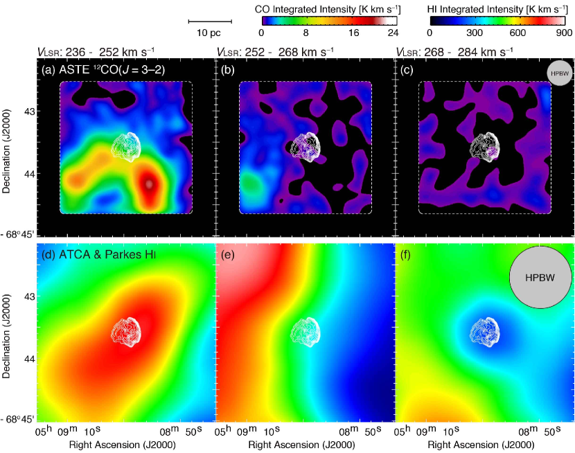
Figure 2: Velocity channel maps of (a–c) ASTE ¹²CO($J$ = 3–2) and (d–f) ATCA $\&$ Parkes Hi. The integration velocity range is $V_{\mathrm{LSR}}$ = 236–252 km s^-1 for Figures 2(a) and 2(d), $V_{\mathrm{LSR}}$ = 252–268 km s^-1 for Figures 2(b) and 2(e), and $V_{\mathrm{LSR}}$ = 268–284 km s^-1 for Figures 2(c) and 2(f). Superposed contours represent Chandra X-rays in the energy band from 0.3–7.0 keV. The contour levels are 1.0, 1.5, 2.1, 2.8, 3.6, 4.5, 5.5, 6.6, 7.8, and $9.0\times 10^{-6}$ photons s^-1 pixel^-1. The beam sizes of CO and Hi are shown in Figures 2(c) and 2(f), respectively. The dashed lines in Figures 2(a–c) indicate the observed area of CO.

3 Results

3.1 Large-Scale Distribution of the X-rays, CO, and Hi

Figure 1a shows a three-color X-ray image of the LMC SNR N103B as observed by Chandra (e.g., Lewis et al., 2003). The soft-band X-rays (red: 0.3–0.6 keV) are bright in the western shell, while the medium-band X-rays (green: 0.6–0.9 keV) and hard-band X-rays (blue: 0.9–7.0 keV) show a similar brightness in both the western and eastern half. The northwestern shell has a spherical edge in the soft-band X-rays, whereas the southeastern shell is strongly deformed especially toward the regions at ($\alpha_{\mathrm{J2000}}$, $\delta_{\mathrm{J2000}}$) $\sim$ ($05^{\mathrm{h}}09^{\mathrm{m}}00^{\mathrm{s}}$, $-68\arcdeg 43\arcmin 43\arcsec$) and at $\sim$ ($05^{\mathrm{h}}08^{\mathrm{m}}58^{\mathrm{s}}$, $-68\arcdeg 43\arcmin 46\arcsec$). The X-ray bright spots are also located not only in the shell interior around ($\alpha_{\mathrm{J2000}}$, $\delta_{\mathrm{J2000}}$) $\sim$ ($05^{\mathrm{h}}09^{\mathrm{m}}58\fs 0$, $-68\arcdeg 43\arcmin 33\arcsec$), but also in the western shell at ($\alpha_{\mathrm{J2000}}$, $\delta_{\mathrm{J2000}}$) $\sim$ ($05^{\mathrm{h}}08^{\mathrm{m}}58\fs 0$, $-68\arcdeg 43\arcmin 28\arcsec$), $\sim$ ($05^{\mathrm{h}}08^{\mathrm{m}}58\fs 0$, $-68\arcdeg 43\arcmin 35\arcsec$), and $\sim$ ($05^{\mathrm{h}}08^{\mathrm{m}}58\fs 3$, $-68\arcdeg 43\arcmin 33\arcsec$) (see dashed circles in Figure 1a). These X-ray spots are also bright in the H$\alpha$ emission. Figure 1b shows an H$\alpha$ image obtained using Hubble Space Telescope (HST) with WFC3. We see prominent optical nebular knots (I), (II), (III), and (IV) defined as (Li et al., 2017, dashed circles in Figure 1b). The diffuse H$\alpha$ emission is seen in only the western half of the SNR, similar to the soft-band X-ray distribution.

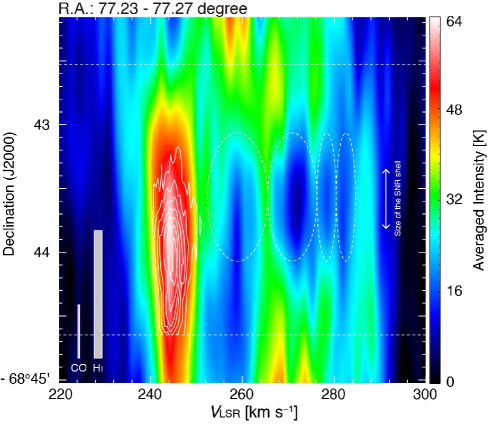
Figure 3: Position–velocity diagram of ATCA $\&$ Parkes Hi (color image) and ASTE ¹²CO($J$ = 3–2) (contours). The integration velocity range in Right Ascension is from 77.23 to 77.27 degrees, corresponding to the HPBW of Hi data ($\sim 60^{\prime\prime}$). The lowest contour level and contour intervals are 0.28 K ($\sim 7\sigma$). The beam size and velocity resolution are also shown. Horizontal lines represent observed boundaries of CO. Dashed circles indicate the Hi hole-like structures in the velocity space. The vertical arrow indicates the size of the SNR shell.

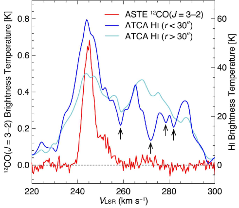
Figure 4: Averaged profiles of ¹²CO($J$ = 3–2) (red) and Hi (blue and cyan) toward the SNR N103B. The regions averaged the cyan and blue spectra are the outside and inside of the circle with a radius of $30^{\prime\prime}$ at the center position of ($\alpha_{\mathrm{J2000}}$, $\delta_{\mathrm{J2000}}$) $\sim$ ($05^{\mathrm{h}}08^{\mathrm{m}}59^{\mathrm{s}}$, $-68\arcdeg 43\arcmin 36\arcsec$). The boundaries averaged both the CO and Hi spectra are the map size of Figure 2.

Figure 2 shows the velocity channel maps of ¹²CO($J$ = 3–2) and Hi obtained using ASTE and ATCA & Parkes, respectively. We confirmed an existence of GMC in the south of the SNR, previously mentioned by Sano et al. (2017a, 2018). The size of GMC is $\sim$30 pc $\times$ 20 pc with an arc-like morphology. The southern edge of the SNR appears to be along the GMC in the velocity range of 236–252 km s^-1 (see Figure 2a). We newly find an HI cloud in the same velocity of the GMC (Figure 2d). To derive the mass of the Hi cloud, we use the following equation (Dickey & Lockman, 1990):

$$N_{\mathrm{p}}(\mathrm{H}{\textsc{i}})=1.823\times 10^{18}\;W(\mathrm{H}{\textsc{i}})\;(\mathrm{cm}^{-2}),$$ (1)

where $N_{p}$(Hi) is the proton column density of Hi and $W$(Hi) is the integrated intensity of Hi. We finally obtain the mass of the Hi cloud is $\sim$$2\times 10^{4}$ $M_{\sun}$, which is significantly smaller than that of the GMC ($\sim$$10^{6}$ $M_{\sun}$). We also note that the diffuse Hi gas is also seen in the velocity of $V_{\mathrm{LSR}}>250$ km s^-1. For the Hi map of the velocity of 268–284 km s^-1, the Hi integrated intensity is decreased toward the SNR (see Figure 2f). The size of intensity-decreased region coincides with the beam size of Hi data.

Figure 3 shows position-velocity diagrams of Hi and CO. The peak velocity of GMC is quite similar to that of Hi cloud ($V_{\mathrm{LSR}}\sim$244 km s^-1). We also find four cavity-like structures of Hi in the position-velocity diagram (see dashed circles in Figure 3). The cavity-like structures are centered at the position of the SNR in declination. The sizes of them are similar to the beam size of Hi. This indicates that the Hi gas at the velocity of $V_{\mathrm{LSR}}>250$ km s^-1 is observed as the Hi absorption line owing to the strong radio continuum emission from the SNR, and hence is located in front of the SNR. A similar case is also seen in the LMC SNRs N49 (Yamane et al., 2018). The Hi profiles also support this idea. Figure 4 shows the CO and Hi profiles toward the SNR N103B. We find significant differences between the ambient Hi gas (cyan, outside of the SNR) and the Hi gas in the direction of the SNR (blue, inside of the SNR). The velocities of absorption lines indicated by the four arrows roughly coincide with the central velocities of the Hi cavity-like structures as shown in Figure 3. We also find the line broadening of CO at the velocity range from $\sim$248 to $\sim$260 km s^-1, implying a possible evidence for the acceleration of part of the GMC. In the present paper, we therefore focus on the GMC and Hi cloud at the velocity around 250 km s^-1, which are likely associated with the SNR.

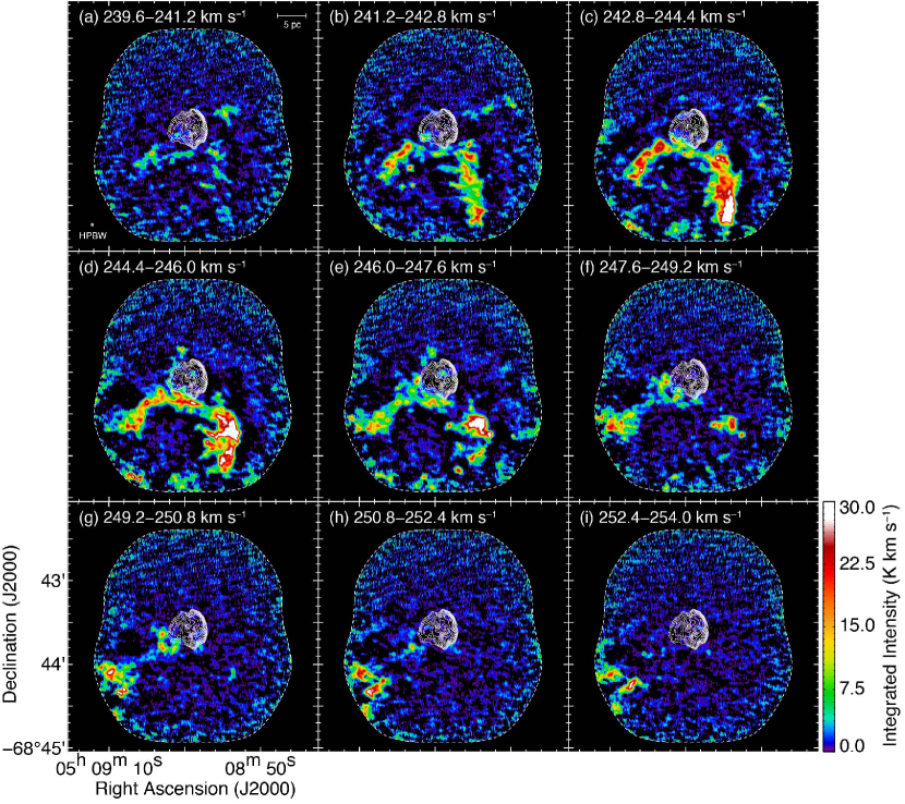
Figure 5: Velocity channel map of the ALMA ¹²CO($J$ = 1–0) superposed on the Chandra X-ray contours as in Figure 2. Each panel shows CO intensity distribution integrated every 1.6 km s^-1 in a velocity range from 239.6 to 254.0 km s^-1. The regions enclose by the dashed lines indicate the observed areas using ALMA.

3.2 Detailed CO Distribution with ALMA

Figure 5 shows velocity channel maps of ¹²CO($J$ = 1–0) line emission obtained with ALMA, where the Chandra X-ray contours are superposed. Each map taken every 1.6 km s^-1 from $V_{\mathrm{LSR}}$ = 239.6–254.0 km s^-1. The GMC in N103B is spatially resolved into many CO filaments and clouds, and only part of the GMC is associated with the SNR. For the velocity range of $V_{\mathrm{LSR}}$ = 244.4–246.0 km s^-1 (Figure 5d), CO filaments and the edge of the GMC completely delineate the outer boundary of the SNR from south to northeast in a clockwise direction. This trend is also seen at the velocity range of $V_{\mathrm{LSR}}$ = 246.0–252.4 km s^-1 (Figures 5e–5h). We note that tiny molecular clumps at ($\alpha_{\mathrm{J2000}}$, $\delta_{\mathrm{J2000}}$) $\sim$ ($05^{\mathrm{h}}08^{\mathrm{m}}58\fs 9$, $-68\arcdeg 43\arcmin 31\arcsec$) (hereafter referred to as “clump A”), and at ($\alpha_{\mathrm{J2000}}$, $\delta_{\mathrm{J2000}}$) $\sim$ ($05^{\mathrm{h}}08^{\mathrm{m}}58\fs 1$, $-68\arcdeg 43\arcmin 46\arcsec$) (hereafter referred to as “clump B”). The clump A appears to be embedded within the SNR, while the clump B is associated with the edge of the southwestern shell.

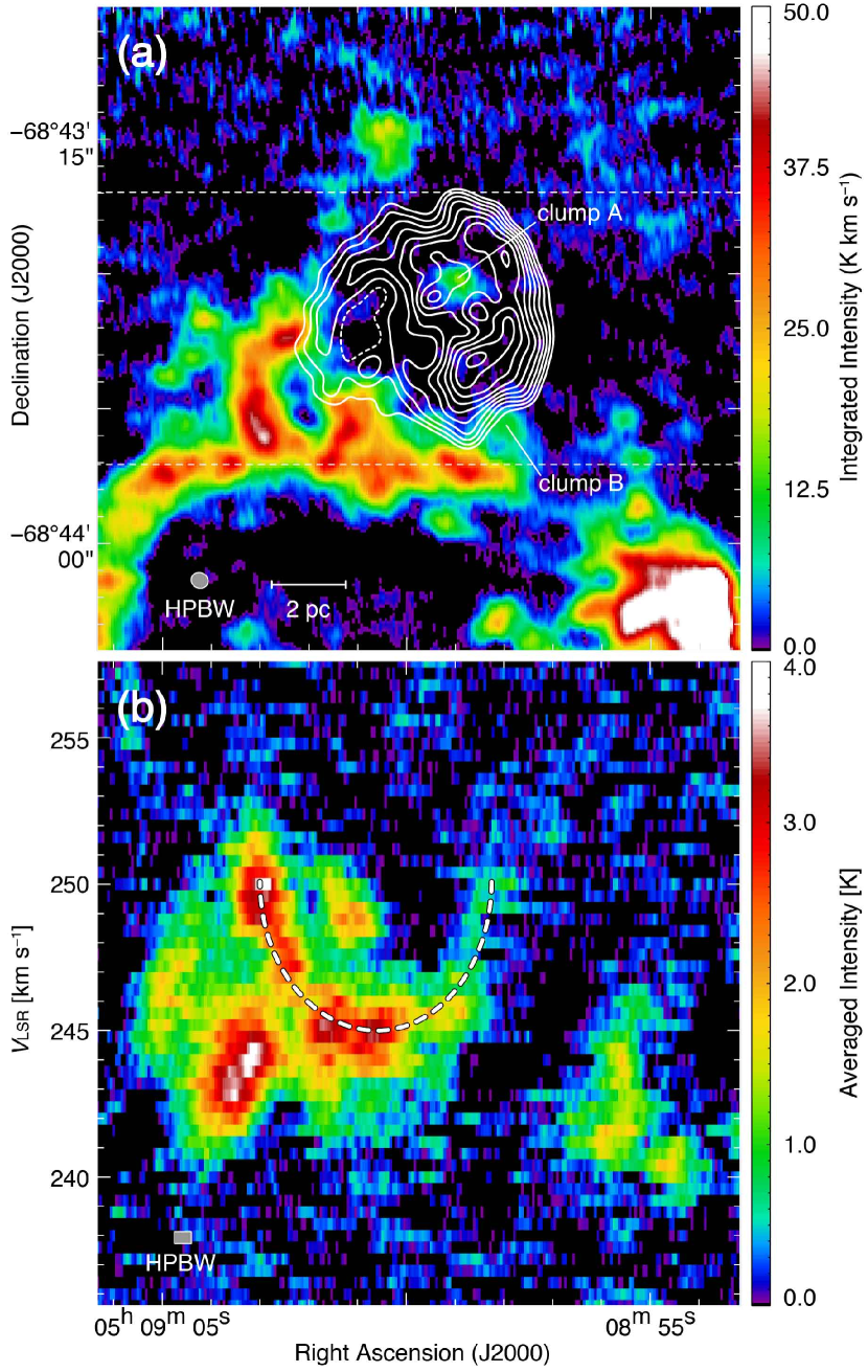
Figure 6: (a) Integrated intensity map of ALMA ¹²CO($J$ = 1–0) superposed on the Chandra X-ray contours. The integration velocity range is from 244.8 to 252.8 km s^-1. The contour levels are the same as in Figure 2. The tiny molecular clumps A and B are also shown. (b) Position–velocity diagram of the ALMA ¹²CO($J$ = 1–0). The integration range in Declination is from $-68\arcdeg 43\arcmin 51\arcsec$ to $-68\arcdeg 43\arcmin 21\arcsec$, corresponding to the dashed lines in Figure 6a. The dashed-curve represents an expanding gas motion.

Figure 6a shows an enlarged view of the ¹²CO($J$ = 1–0) distribution in a velocity range from $V_{\mathrm{LSR}}$ = 244.8–252.8 km s^-1. The molecular clouds show a remarkably good spatial correlation with the SNR shell from southwest to northeast in clockwise direction, indicating that the molecular clouds are likely associated with the SNR shockwaves. By contrast, no molecular clouds are detected in the northwestern shell except for the tiny molecular clump embedded within the shell. Figure 6b shows a position-velocity diagram of ¹²CO($J$ = 1–0) with the integration range from $-68\arcdeg 43\arcmin 51\arcsec$ to $-68\arcdeg 43\arcmin 21\arcsec$ in Declination (see dashed lines in Figure 6a). We find a cavity-like structure in the position-velocity diagram, indicating an evidence for the expanding gas motion with an expansion velocity of $\sim$5 km s^-1 (see the dashed-curve in Figure 6b). The spatial extent of cavity-like structure is roughly similar to the shell size of the SNR.

To estimate the mass of molecular clouds, we use the following equation:

$$M=\mu m_{\mathrm{p}}D^{2}\Omega\sum_{i}[N_{i}(\mathrm{H}_{2})],$$ (2)

where $\mu$ is the mean molecular weight relative to the atomic hydrogen, $m_{\mathrm{p}}$ is the mass of atomic hydrogen, $D$ is the distance to the molecular cloud, $\Omega$ is the solid angle of a pixel, and $N_{i}(\mathrm{H}_{2})$ is the molecular hydrogen column density for each pixel $i$. We use $\mu=2.38$ by taking into account the helium abundance $\sim$36% to the molecular hydrogen mass (c.f., Fukui et al., 2008). The molecular hydrogen column density $N(\mathrm{H}_{2})$ is given by using the relation:

$$N(\mathrm{H}_{2})=X\cdot W(^{12}\mathrm{CO}),$$ (3)

where $X$ is the conversion factor in the unit of cm^-2 (K km s${}^{-1})^{-1}$ and $W(^{12}\mathrm{CO})$ is the integrated intensity of the ¹²CO($J$ = 1–0) line emission in the unit of K km s^-1. We use the conversion factor $X=7.0\times 10^{20}$ cm^-2 (K km s^-1)^-1 (Fukui et al., 2008). The physical properties of molecular clouds are estimated for the regions that are significantly detected by CO line emission with a 3-sigma or higher. The size of molecular cloud is defined as $(A/\pi)^{0.5}\times 2$, where $A$ is the total surface area of the molecular cloud enclosed by the 3-sigma level. We finally derive the total mass of the molecular cloud of $\sim$$8\times 10^{5}$ $M_{\sun}$, which is roughly consistent with previous CO studies (Sano et al., 2017a, 2018).

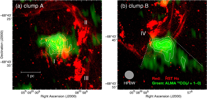
Figure 7: Maps of HST H$\alpha$ intensity (red color) and integrated intensity of the ALMA ¹²CO($J$ = 1–0) (green color) toward (a) clump A and (b) clump B. The integration velocity range is 244.8 to 248.0 km s^-1 for clump A and is 249.2 to 252.0 km s^-1 for clump B. Superposed contours indicate the CO intensity and are plotted from 4 K km s^-1 with 2 K km s^-1 steps. We also showed the optical nebular knots (I), (II), (III), and (IV) as defined by Li et al. (2017).

3.3 Tiny Molecular Clumps Associated with the Optical Nebula Knots

Figure 7 shows enlarged views toward tiny molecular clumps A and B. Red and green images represent the HST H$\alpha$ and ALMA ¹²CO($J$ = 1–0) integrated intensity, respectively. We find that the tiny molecular clumps A and B are located near the optical nebular knots (I) and (II), which are also bright in the soft-band X-rays, respectively (see Figure 1a). In contrast, there are no CO counterparts for other optical nebular knots (II) and (III) in Figure 7a. Since the tiny clumps have extended distributions compared with the beam size of ALMA, we assumed a beam-filling factor of $\sim$1. Using the equations (2) and (3), the size, mass, and density are therefore estimated to be $\sim$110 $M_{\sun}$, $\sim$1.2 pc, and $\sim$2000 cm^-3 for clump A; $\sim$90 $M_{\sun}$, $\sim$1.3 pc, and $\sim$1400 cm^-3 for clump B. We also note that the molecular clump B shows a V-shaped structure pointing toward the center of the SNR (see dashed lines in Figure 7b), which will be discussed later.

4 Discussion

4.1 Inhomogeneous Distribution of the Interstellar Gas

The dynamical interaction between the SNR shocks and the ISM affects the evolution of SNRs through a strong deformation of the shell morphology, if the ISM is dense enough (e.g., RX J1713.7$-$3946, Fukui et al. 2003; Kes 79, Kuriki et al. 2017). On the other hand, Type Ia SNRs usually evolve in the low-density ambient medium, and hence form a relatively symmetric morphology (Lopez et al., 2009). According to Roper et al. (2018), the LMC Type Ia SNR J0509$-$6731 shows a symmetry shell with an isotropic expansion velocity of $\sim$$7500\pm 1700$ km s^-1 derived by the proper motion studies in X-rays. No dense molecular cloud is detected toward the SNR and the column density of Hi is estimated to be $\sim$4–$6\times 10^{20}$ cm^-2, indicating a very low-density interstellar environment. In this section, we discuss the interstellar environment in the Type Ia SNR N103B and its relation with the shell morphology.

Based on the ALMA results, the CO clouds—a part of the GMC—are physically associated with the SNR N103B. The CO clouds delineate the outer boundary of the SNR from southwest to northeast in clockwise direction, while the northwestern shell has no CO clouds (see Figures 5 and 6a). Although the spatial resolution is limited of Hi data ($\sim$15 pc), we estimate the peak column density of Hi is $\sim$$2\times 10^{21}$ cm^-2. We argue that the inhomogeneous CO distribution and gas rich environment possibly affect the X-ray shell-morphology of the SNR. In fact, the northwestern edge of X-ray shell shows a spherical shape, whereas the southeastern shell appears to be strongly deformed (see Figure 1a). Moreover, a difference of shock velocity for each region has been observed. According to Ghavamian et al. (2017), the velocity for Balmer-dominant shocks is $\sim$2100 km s^-1 in the northern edge of the shell, in which no molecular clouds are seen. On the other hand, the slow shock velocity of $\sim$1200 km s^-1 is observed in the southwestern edge of the SNR where the tiny molecular clump B is embedded (see Figures 6a and 7b). Invoking ram pressure conservation ($\rho V_{\mathrm{sh}}^{2}$ = constant), we expect that the ISM density of the southeastern shell is at least three times higher than that of the northern shell. To verify the interpretation, further Hi observations with high spatial resolution with a few pc scales are needed. In addition, direct measurements of shock velocity using the proper motion technique is useful to compare the inhomogeneity of the ISM associated with the SNR.

Moreover, the origin of inhomogeneous gas distribution is possibly related with the stellar environment. In fact, the SNR is projected near the double star cluster NGC 1850, which contains a young ($50\pm 10$ Myr) globular-like star cluster and an even younger ($4.3\pm 0.9$ Myr) small cluster (e.g., Gilmozzi et al., 1994). Figure 8a shows the optical image around the SNR N103B obtained with the Very Large Telescope (VLT). The globular-like star cluster NGC 1850 is located toward the southwest of N103B with a projected separation between them of $\sim$30 pc, indicating that the molecular clouds surrounding N103B are affected by the stellar feedback from the star clusters. Someya et al. (2014) also suggested the physical association of N103B and NGC 1850 by X-ray spectroscopic analysis. On the other hand, Maggi et al. (2016) argued that the spatial coincidence between the H$\alpha$ nebula and the SNR is likely a projection effect. They concluded that the SNR is located on the far side of the LMC as suggested by its large fraction of $N_{\mathrm{p}}$(X-rays) / $N_{\mathrm{p}}$(Hi), where $N_{\mathrm{p}}$(X-rays) is the absorbing column density of N103B. However, the fraction is underestimated because they did not take into account the molecular hydrogen as the ISM component. We claim that the SNR N103B is located on the similar distance of the globular-like star cluster NGC 1850. Figure 8b shows the Spitzer IRAC 8 $\mu$m image toward N103B superposed on the CO contours. We find that the bright spots in 8 $\mu$m—yellow or red colors in Figure 8b—are located only the southwestern edges of molecular clouds except for the direction of the SNR. Since the Spitzer IRAC 8 $\mu$m image is dominated by polycyclic aromatic hydrocarbon (PAH) line emission, this trend may be understood with the UV excitation by the massive star clusters. Future ALMA and SOFIA observations with [Ci] and [Cii] will allow us to study physical properties of PDR under the strong feedback in addition to the origin of the inhomogeneous gas distribution.

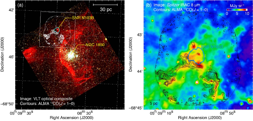
Figure 8: (a) Optical image of NGC 1850 taken with the Very Large Telescope (VLT). The red, green, and blue represent H$\alpha$, V-, and, B-bands respectively (credit: ESO). White contours indicate the ALMA ¹²CO($J$ = 1–0) integrated intensity ($V_{\mathrm{LSR}}$ = 244.8–252.8 km s^-1) and the lowest contour level and contour intervals are 10 K km s^-1. The dashed contour represents the Chandra X-ray boundary at the level of $0.2\times 10^{-5}$ photons s^-1 pixel^-1. The rectangle box indicates the region shown in Figure 8b. (b) SAGE Spitzer IRAC 8 $\mu$m image toward the SNR N103B (Meixner et al., 2006). The superposed contours are the same as in Figure 8a.

4.2 Implications for the progenitor system of N103B

SNR N103B is one of the most promising candidates for the SD hypothesis, that is, for having a progenitor system consisting of a white dwarf and a non-degenerate companion (e.g., Williams et al., 2014; Li et al., 2017; Ghavamian et al., 2017). The SD progenitor system may produce optically thick winds—named as accretion winds—from the white dwarf when the mass accretion rate is higher than the stable nuclear fusion rate (e.g., Hachisu et al., 1996, 1999a, 1999b). If this is true, the expanding gas motion of the ISM can be observed similarly to the other Type Ia SNRs: RCW 86 and Tycho (Sano et al., 2017c; Chen et al., 2017). We here discuss the progenitor system of N103B based on the ALMA CO results of the associated interstellar molecular gas.

First, we argue that the expanding shell of CO cloud (Figure 6b) is roughly consistent with the acceleration by only the accretion winds of the progenitor system of N103B. Based on the ALMA CO results and the equations (2) and (3), the mass of expanding shell is estimated to be $\sim$$5\times 10^{3}$ $M_{\sun}$. Since the expansion velocity of CO is $\sim$5 km s^-1, the momentum is calculated to be $\sim$$2.5\times 10^{4}$ $M_{\sun}$ km s^-1. According to Hachisu et al. (1999a, b), the accretion wind of Type Ia SD progenitor system has a wind mass of $\sim$ $10^{-4}$ $M_{\sun}$ yr^-1 and a wind velocity of $\sim$2000 km s^-1 as maximum values (see also Nomoto et al., 2005). Assuming the wind duration of $\sim$ $3\times 10^{5}$ yr, the momentum of total accretion wind is to be $\sim$$6\times 10^{4}$ $M_{\sun}$ km s^-1. It is therefore that $\sim$40% of the wind momentum had transferred to the expanding gas motion. The percentage of momentum transfer is slightly larger than a theoretical calculation in an ideal adiabatic wind shell (e.g., Weaver et al., 1977), but is not impossible. In addition to this, the CO cloud is possibly accelerated by the shock wave of N103B even though the young age of 380–860 yr (Rest et al., 2005). According to Zhou et al. (2016), a possible line broadening of CO emission is detected in the young SNR Tycho with an age of 446 yr. To test the gas acceleration and line broadening in N103B, we need more sensitive CO observations with fine spatial resolutions with ALMA.

We also note that the V-shaped structure of tiny molecular clump B is possibly evidence for a blown-off cloud that has overtaken the accretion winds from the progenitor system. According to Fukui et al. (2017), a similar V-shaped structure of Hi/CO clouds is observed in the Galactic core-collapse SNR Vela Jr. The authors conclude that a V-shaped Hi tail with a dense head of CO survived against the stellar wind from the massive progenitor. Since the accretion wind of N103B is weaker than the stellar wind of Vela Jr, the V-shaped structure of N103B was possibly formed by the accretion wind because of the high wind speed up to $\sim$2000 km s^-1 and the large wind duration.

In conclusion, we propose a possible scenario that N103B exploded in the wind-bubble formed by the accretion winds from the progenitor system, and is now interacting with the dense wind-cavity of the molecular clouds. This scenario is consistent with the SD origin of N103B. To confirm the scenario, a reliable identification of companion a star is needed.

5 Conclusions

We have carried out new ¹²CO($J$ = 1–0, 3–2) observations using ALMA and ASTE in order to spatially resolve molecular clouds associated with the Type Ia SNR N103B in the LMC. The primary conclusions of the present study are summarized as below.

1. We have confirmed the existence of GMC at $V_{\mathrm{LSR}}$ $\sim$245 km s^-1 toward the southeast of the SNR using the ¹²CO($J$ = 3–2) data at the spatial resolution of $\sim$6 pc. Using the ALMA ¹²CO($J$ = 1–0) data, we have spatially resolved CO clouds along the southeastern shell of the SNR with the spatial resolution of $\sim$0.4 pc. The CO clouds show the expanding gas motion in the position-velocity diagram with the expansion velocity of $\sim$5 km s^-1. The spatial extent of expanding shell is roughly similar to the size of the SNR. On the other hand, there are no molecular clouds toward the northwestern shell of the SNR. We also revealed tiny molecular clumps associated with the optical nebula knots, the size and mass of which are estimated to be $\sim$100 $M_{\sun}$ and $\sim$1 pc, respectively.

2. We have argued that the asymmetric morphology of the X-ray shell is possibly related to the inhomogeneous distribution of the ISM. For the northwestern region, the SNR has the spherical shell in X-rays because there are no dense molecular clouds. On the other hand, the southeastern shell is strongly deformed owing to the shock interaction with the dense molecular clouds. The shock-velocities derived by optical emission are also consistent with the inhomogeneous density distribution of the ISM. To verify the interpretation, both the further Hi observations with fine spatial resolution and the direct measurements of shock velocity—e.g., proper motion measurements—are needed.

3. We have presented a possible scenario that N103B exploded in the wind-bubble formed by the accretion winds from the progenitor system, and is now interacting with the wind-cavity of the molecular gas. Because the momentum of the expanding gas motion can be explained by the energy input of the accretion wind from the SD progenitor system. To confirm the scenario, a reliable identification of companion a star is needed.

References

- Banas et al. (1997) Banas, K. R., Hughes, J. P., Bronfman, L., & Nyman, L.-Å. 1997, ApJ, 480, 607
- Bozzetto et al. (2017) Bozzetto, L. M., Filipović, M. D., Vukotić, B., et al. 2017, ApJS, 230, 2
- Blair et al. (2007) Blair, W. P., Ghavamian, P., Long, K. S., et al. 2007, ApJ, 662, 998
- Chen et al. (2017) Chen, X., Xiong, F., & Yang, J. 2017, A&A, 604, A13
- Cornwell (2008) Cornwell, T. J. 2008, IEEE Journal of Selected Topics in Signal Processing, 2, 793
- Dickey & Lockman (1990) Dickey, J. M., & Lockman, F. J. 1990, ARA&A, 28, 215
- Douvion et al. (2001) Douvion, T., Lagage, P. O., Cesarsky, C. J., & Dwek, E. 2001, A&A, 373, 281
- Ezawa et al. (2004) Ezawa, H., Kawabe, R., Kohno, K., & Yamamoto, S. 2004, Proc. SPIE, 5489, 763
- Fukui et al. (2003) Fukui, Y., Moriguchi, Y., Tamura, K., et al. 2003, PASJ, 55, L61
- Fukui et al. (2008) Fukui, Y., Kawamura, A., Minamidani, T., et al. 2008, ApJS, 178, 56
- Fukui et al. (2017) Fukui, Y., Sano, H., Sato, J., et al. 2017, ApJ, 850, 71
- Fruscione et al. (2006) Fruscione, A., McDowell, J. C., Allen, G. E., et al. 2006, Proc. SPIE, 6270, 62701V
- Ghavamian et al. (2017) Ghavamian, P., Seitenzahl, I. R., Vogt, F. P. A., et al. 2017, ApJ, 847, 122
- Gilmozzi et al. (1994) Gilmozzi, R., Kinney, E. K., Ewald, S. P., Panagia, N., & Romaniello, M. 1994, ApJ, 435, L43
- Hachisu et al. (1996) Hachisu, I., Kato, M., & Nomoto, K. 1996, ApJ, 470, L97
- Hachisu et al. (1999a) Hachisu, I., Kato, M., & Nomoto, K. 1999a, ApJ, 522, 487
- Hachisu et al. (1999b) Hachisu, I., Kato, M., Nomoto, K., & Umeda, H. 1999b, ApJ, 519, 314
- Hachisu et al. (2008) Hachisu, I., Kato, M., & Nomoto, K. 2008, ApJ, 679, 1390
- Hughes et al. (1995) Hughes, J. P., Hayashi, I., Helfand, D., et al. 1995, ApJ, 444, L81
- Iben & Tutukov (1984) Iben, I., Jr., & Tutukov, A. V. 1984, ApJS, 54, 335
- Kasen (2010) Kasen, D. 2010, ApJ, 708, 1025
- Katsuda et al. (2015) Katsuda, S., Mori, K., Maeda, K., et al. 2015, ApJ, 808, 49
- Kim et al. (2003) Kim, S., Staveley-Smith, L., Dopita, M. A., et al. 2003, ApJS, 148, 473
- Kuriki et al. (2017) Kuriki, M., Sano, H., Kuno, N., et al. 2017, arXiv:1711.08165
- Lewis et al. (2003) Lewis, K. T., Burrows, D. N., Hughes, J. P., et al. 2003, ApJ, 582, 770
- Li et al. (2017) Li, C.-J., Chu, Y.-H., Gruendl, R. A., et al. 2017, ApJ, 836, 85
- Maggi et al. (2016) Maggi, P., Haberl, F., Kavanagh, P. J., et al. 2016, A&A, 585, A162
- Martínez-Rodríguez et al. (2017) Martínez-Rodríguez, H., Badenes, C., Yamaguchi, H., et al. 2017, ApJ, 843, 35
- McMullin et al. (2007) McMullin, J. P., Waters, B., Schiebel, D., Young, W., & Golap, K. 2007, Astronomical Data Analysis Software and Systems XVI, 376, 127
- Meixner et al. (2006) Meixner, M., Gordon, K. D., Indebetouw, R., et al. 2006, AJ, 132, 2268
- Minamidani et al. (2011) Minamidani, T., Tanaka, T., Mizuno, Y., et al. 2011, AJ, 141, 73
- Nomoto (1982) Nomoto, K. 1982, ApJ, 257, 780
- Nomoto et al. (2005) Nomoto, K., Suzuki, T., Deng, J., Uenishi, T., & Hachisu, I. 2005, 1604-2004: Supernovae as Cosmological Lighthouses, 342, 105
- Lopez et al. (2009) Lopez, L. A., Ramirez-Ruiz, E., Badenes, C., et al. 2009, ApJ, 706, L106
- Paczynski (1985) Paczynski, B. 1985, Cataclysmic Variables and Low-Mass X-ray Binaries, 113, 1
- Perlmutter et al. (1999) Perlmutter, S., Aldering, G., Goldhaber, G., et al. 1999, ApJ, 517, 565
- Rest et al. (2005) Rest, A., Suntzeff, N. B., Olsen, K., et al. 2005, Nature, 438, 1132
- Roper et al. (2018) Roper, Q., Filipovi, M., Allen, G. E., et al. 2018, MNRAS,
- Sano et al. (2015) Sano, H., Fukui, Y., Yoshiike, S., et al. 2015, Revolution in Astronomy with ALMA: The Third Year, 499, 257
- Sano et al. (2017a) Sano, H., Fujii, K., Yamane, Y., et al. 2017a, 6th International Symposium on High Energy Gamma-Ray Astronomy, 1792, 040038
- Sano et al. (2017b) Sano, H., Yamane, Y., Voisin, F., et al. 2017b, ApJ, 843, 61
- Sano et al. (2017c) Sano, H., Reynoso, E. M., Mitsuishi, I., et al. 2017c, Journal of High Energy Astrophysics, 15, 1
- Sano et al. (2018) Sano, H. et al. 2018, in preparation
- Someya et al. (2014) Someya, K., Bamba, A., & Ishida, M. 2014, PASJ, 66, 26
- Sorai et al. (2000) Sorai, K., Sunada, K., Okumura, S. K., et al. 2000, Proc. SPIE, 4015, 86
- Webbink (1984) Webbink, R. F. 1984, ApJ, 277, 355
- Weaver et al. (1977) Weaver, R., McCray, R., Castor, J., Shapiro, P., & Moore, R. 1977, ApJ, 218, 377
- Whelan & Iben (1973) Whelan, J., & Iben, I., Jr. 1973, ApJ, 186, 1007
- Williams et al. (2012) Williams, B. J., Borkowski, K. J., Reynolds, S. P., et al. 2012, ApJ, 755, 3
- Williams et al. (2014) Williams, B. J., Borkowski, K. J., Reynolds, S. P., et al. 2014, ApJ, 790, 139
- Wong et al. (2011) Wong, T., Hughes, A., Ott, J., et al. 2011, ApJS, 197, 16
- Wong et al. (2017) Wong, T., Hughes, A., Tokuda, K., et al. 2017, ApJ, 850, 139
- Yamaguchi et al. (2014) Yamaguchi, H., Badenes, C., Petre, R., et al. 2014, ApJ, 785, L27
- Yamane et al. (2018) Yamane, Y., Sano, H., van Loon, J. T., et al. 2018, ApJ, 863, 55
- Zhou et al. (2016) Zhou, P., Chen, Y., Zhang, Z.-Y., et al. 2016, ApJ, 826, 34