Calculation of higher-order moments by higher-order tensor renormalization group

Abstract

A calculation method for higher-order moments of physical quantities, including magnetization and energy, based on the higher-order tensor renormalization group is proposed. The physical observables are represented by impurity tensors. A systematic summation scheme provides coarse-grained tensors including multiple impurities. Our method is compared with the Monte Carlo method on the two-dimensional Potts model. While the nature of the transition of the $q$-state Potts model has been known for a long time owing to the analytical arguments, a clear numerical confirmation has been difficult due to extremely long correlation length in the weakly first-order transitions, e.g., for $q=5$. A jump of the Binder ratio precisely determines the transition temperature. The finite-size scaling analysis provides critical exponents and distinguishes the weakly first-order and the continuous transitions.

1 Introduction

Tensor networks (TN) are powerful tools for strongly correlated many-body physics [1, 2]. As a pioneering work, the density matrix renormalization group (DMRG) [3] achieves great success in one-dimensional quantum systems. This method can be viewed as a variational method based on the matrix product states formalism, i.e. the one-dimensional TN states. The projected entangled pair state (PEPS) [4] and the projected entangled simplex state (PESS) [5] provide its generalization to higher-dimensional systems.

The tensor renormalization group method (TRG) [6] provides an efficient contraction scheme avoiding exponential divergence of the bond dimension based on coarse-graining TNs. Many derivatives are proposed as a more efficient and accurate method [7, 8, 9, 10, 11]. The higher-order tensor renormalization group method (HOTRG) is a TN method applicable to a higher-dimensional system [9, 12]. The higher-order singular value decomposition (HOSVD) provides its truncation scheme. An isometry which merges two bonds into one bond plays a key role in information compression. It is another advantage of HOTRG than other TN renormalization methods because a local original tensor is not decomposed into two tensors.

The partition function of a classical system can be represented by a TN [13, 8]. Thus the free energy is quite accurately estimated by using real-space renormalization group methods mentioned above. There are two ways to calculate an expectation value of a physical quantity like magnetization $\langle m\rangle$. One method is numerical differentiation of the free energy with respect to a model parameter, for example, the external magnetic field. The other is introduction of an “impurity”; an expectation value is represented by a TN in which one of tensors is replaced with an impurity tensor that represents the local order parameter.

Higher moments of physical quantity are important for analysis of critical phenomena. Expectation value of the squared magnetization, $\langle m^{2}\rangle$, is regarded as an order parameter. The Binder ratio is typically used to determine the transition point in the Monte Carlo (MC) simulations [14]. Finite-size scaling analysis of these quantities provides critical exponents. However, calculation methods of higher moments are limited and not accurate in TN methods. In the numerical differentiation method, we need to calculate higher-order derivative to estimate a higher-order moment. Numerically it causes cancellation of significant digits. Especially near the phase transition point, the higher-order derivative shows a sharp change and it is difficult to assure its accuracy. An efficient scheme for the TN states was proposed based on the momentum generating functions [15]. However it also needs the numerical differentiation with respect to an indeterminate to extract a moment. On the other hand, the impurity method also has a problem. Let us assume that a system has a transitional symmetry and consider a physical quantity represented as a spacial average of local quantities, for example $m=(1/N)\sum_{i=1}^{N}\sigma_{i}$. Only one TN which contains one impurity tensor is sufficient to estimate its expectation value, $\langle m\rangle$. However, for the second-order moment, all spatial configurations of two impurities are necessary. Therefore, since the number of TNs corresponding to two-point correlation functions diverges, such an approach is unmanageable. An exception is a one-dimensional system, where matrix product operator representation for the high-order moments is known [16].

In this paper, we propose an alternative way of calculating the higher-order moments by introducing the impurity tensors into the HOTRG scheme. We define a coarse-grained tensor which represents summation of all configurations of multiple impurities. Thus its trace directly yields the higher-order moments. The systematic summation technique proposed for the infinite PEPS method [17] derives the real-space renormalization scheme of the impurity tensor. In contrast to the impurity method mentioned above, the summation over impurity configurations is taken during renormalization steps.

Using our proposed method, we investigate the ferromagnetic $q$-state Potts model [18, 19] on the square lattice. A phase transition between the ferromagnetic and paramagnetic phases is continuous for $q\leq 4$ and discontinuous otherwise. Especially a numerical confirmation of the weakly first-order phase transition in the $5$-state Potts model has attracted much attention [20, 21]. Since the correlation length becomes very large but finite at the transition point, it is difficult to make a distinction between the weakly first-order and second transitions. However, a TN renormalization method can easily treat the huge system size over the correlation length. The corner transfer matrix renormalization group method (CTMRG) [22, 23] can accurately estimate the latent heat of the two-dimensional $5$-state Potts model [24]. The HOTRG approach can confirm the first-order phase transition in the $3$-state Potts model on the simple cubic lattice [12]. In this paper, we present a more systematic method for characterizing the nature of the transition. We perform the HOTRG simulation up to the system size $N=2^{40}$ and show that the second moment of the magnetization clearly distinguishes between discontinuous and continuous phase transitions. Moreover, the finite-size scaling analysis of the Binder ratio accurately produces the critical exponents expected in the first-order phase transition for $q\geq 5$.

In the next section, we present the method for the higher-order moment with a brief introduction of HOTRG. In the third section, we perform numerical simulations in the $q$-state Potts model on a square lattice. We compare our method with a cluster MC method and estimate a transition temperature from a jump of the Binder ratio. In the fourth section, we consider the finite-size scaling ansatz. We estimate the critical exponent from a slope of the Binder ratio at criticality. The last section is devoted to discussions and conclusions.

2 Methods

In general, the partition function of a many-body system has a tensor network representation. For simplicity, let us consider a classical discrete spin system with nearest neighbor interactions on the isotropic square lattice. A generalization to a higher dimensional system is straightforward. If the degrees of freedom are continuous, we use the characterize representation. Then we have

$$Z=\sum_{\{\sigma_{i}\}}\prod_{\langle ij\rangle}W_{\sigma_{i}\sigma_{j}}\prod_{i=1}^{N}V_{\sigma_{i}}=\operatorname{tTr}\prod_{i=1}^{N}T_{x_{i}y_{i}x^{\prime}_{i}y^{\prime}_{i}},$$ (1)

where $W_{\sigma\sigma^{\prime}}$ and $V_{\sigma}$ is the local Boltzmann factor of the nearest neighbor interaction and the magnetic field respectively. A variable $\sigma_{i}$ represents the spin degree of freedom at a site $i$. The local tensor $T$ locates on each lattice site. Based on the eigenvalue decomposition $W=\tilde{U}\Lambda\tilde{U}^{\dagger}$, the local tensor always has the form

$$T_{xyx^{\prime}y^{\prime}}^{(0)}=\sum_{\sigma}X_{\sigma x}X_{\sigma y}X_{\sigma x^{\prime}}^{*}X_{\sigma y^{\prime}}^{*}V_{\sigma},$$ (2)

where $X\equiv\tilde{U}\sqrt{\Lambda}$. The superscript $(0)$ indicates a initial tensor before a renormalization.

Figure 1: Graphical representations of a renormalization step along $y$-axis in HOTRG.

In HOTRG algorithm, the square lattice is contracted along the $x$- and $y$-axes in sequence. The renormalization step with $y$-bond contraction is graphically shown in Fig.1. The renormalized local tensor at the $(t+1)$-th step is calculated as

$$T_{xyx^{\prime}y^{\prime}}^{(t+1)}=\sum_{\begin{subarray}{c}x_{1},x_{1}^{\prime}\\ x_{2},x_{2}^{\prime},y_{1}\end{subarray}}T_{x_{1}yx_{1}^{\prime}y_{1}}^{(t)}T_{x_{2}y_{1}y_{2}^{\prime}y^{\prime}}^{(t)}U_{x_{1}x_{2}x}^{(t)}U_{x_{1}^{\prime}x_{2}^{\prime}x^{\prime}}^{(t)*},$$ (3)

where $U^{(t)}$ is an isometric tensor obtained by the standard HOSVD. In this paper, we abbreviate this contraction as

$$T^{(t+1)}=\mathcal{R}(T^{(t)},T^{(t)};U^{(t)}),$$ (4)

or, when the meaning is clear, more shortly

$$T\leftarrow TT.$$ (5)

We note that a direction of the renormalization depends on a step $t$. The local tensor $T^{(t)}$ after the $t$-th renormalization step represents a system of size $N=2^{t}$. The trace of $T^{(t)}$,

$$Z\simeq\operatorname{Tr}T^{(t)}\equiv\sum_{x,y}T^{(t)}_{xyxy},$$ (6)

yields the partition function of the corresponding finite-size system under the periodic boundary condition.

Figure 2: Renormalization of the impurity tensors with (a) single impurity and (b) two impurities. The impurities are represented by a (orange) circle in the impurity tensors.

First, let us consider the magnetization defined by the average of local magnetization as

$$m\equiv\frac{1}{N}\sum_{i=1}^{N}m_{\sigma_{i}},$$ (7)

where $m_{\sigma_{i}}$ represents a local magnetization at a site $i$. With similar representation to Eq.(2), the corresponding impurity tensor is clearly obtained as

$$S_{1,xyx^{\prime}y^{\prime}}^{(0)}=\sum_{\sigma}X_{\sigma x}X_{\sigma y}X_{\sigma x^{\prime}}^{*}X_{\sigma y^{\prime}}^{*}V_{\sigma}m_{\sigma},$$ (8)

where the additional subscript “$1$” indicates that this impurity tensor contains one impurity in total. In HOTRG, this single impurity tensor is renormalized by using the same isometric tensor $U^{(t)}$ for renormalization of $T^{(t)}$ as

$$\tilde{S}_{1}^{(t+1)}=\mathcal{R}(S_{1}^{(t)},T^{(t)};U^{(t)}).$$ (9)

The trace of this impurity tensor represents a magnetization at a specific site but does not do the averaged magnetization defined in Eq.(7). In order to finally obtain the average over the whole lattice, we should take the local average at each level of the renormalization procedure. Therefore the symmetrized version

$$S_{1}^{(t+1)}=\frac{1}{2}\left\{\mathcal{R}(S_{1}^{(t)},T^{(t)};U^{(t)})+\mathcal{R}(T^{(t)},S_{1}^{(t)};U^{(t)})\right\},$$ (10)

is required, which we write shortly as

$$S_{1}\leftarrow\frac{1}{2}(S_{1}T+TS_{1}).$$ (11)

Its graphical representation is shown in Fig. 2(b). The expectation value of $m$ with the system size $N=2^{t}$ under the periodic boundary condition is estimated by

$$\left\langle m\right\rangle\simeq\frac{\operatorname{Tr}S_{1}^{(t)}}{\operatorname{Tr}T^{(t)}}.$$ (12)

A generalization of this scheme to higher-order moments of the magnetization $\left\langle m^{k}\right\rangle$ is clear. The initial tensors with multiple impurities are defined as

$$S_{k,xyx^{\prime}y^{\prime}}^{(0)}=\sum_{\sigma}X_{\sigma x}X_{\sigma y}X_{\sigma x^{\prime}}^{*}X_{\sigma y^{\prime}}^{*}V_{\sigma}m_{\sigma}^{k}.$$ (13)

The update rule for the two-impurity tensor ($k=2$) can be written as

$$S_{2}\leftarrow\frac{1}{4}\left(S_{2}T+2S_{1}S_{1}+TS_{2}\right),$$ (14)

and its diagram is shown in Fig. 2(b). Obviously $S_{2}$ contains all of the possible configurations of two impurities in a finite system corresponding to the renormalization step. The generalization to more impurities is straightforward as,

$$S_{3}\leftarrow\frac{1}{8}\left(S_{3}T+3S_{2}S_{1}+3S_{1}S_{2}+TS_{3}\right),$$ (15)

$$S_{4}\leftarrow\frac{1}{16}\left(S_{4}T+4S_{3}S_{1}+6S_{2}S_{2}+4S_{1}S_{3}+TS_{4}\right).$$ (16)

The higher-order moment of the magnetization, $\langle m^{k}\rangle$ is calculated by the ratio of $\operatorname{Tr}S_{k}$ to $\operatorname{Tr}T$ similarly to Eq. (12).

Note that we use the same isometric tensor $U^{(t)}$ as for the local tensor regardless of impurity tensors in order to fix the definition of bond indices at each level of renormalization. If we use different isometries for each impurity tensors, they cannot connect properly in the next renormalization step.

So far, we focus on the spacial average of a physical quantity defined at each site but our technique can be applied to a quantity defined on a small cluster, e.g., the interaction energy defined on each pair of spins,

$$e\equiv\frac{1}{N}\sum_{\langle ij\rangle}e_{\sigma_{i}\sigma_{j}}.$$ (17)

To define an impurity tensor for such a impurity located on a bond, it is useful that a change by impurities is absorbed into the local weight $W_{k,\sigma\sigma^{\prime}}\equiv W_{\sigma\sigma^{\prime}}\left(e_{\sigma\sigma^{\prime}}\right)^{k}$. We define $Y_{k}\equiv W_{k}\tilde{U}\Lambda^{-1/2}$ which satisfies $Y_{0}=X$ and $Y_{k}X^{\dagger}=W_{k}$. On these settings, the single and double impurity tensors with impurities on bonds $x$ or $y$ are written as

$$E_{1,xyx^{\prime}y^{\prime}}^{(0)}=\sum_{\sigma}(Y_{1,\sigma x}X_{\sigma y}+X_{\sigma x}Y_{1,\sigma y})X_{\sigma x^{\prime}}^{*}X_{\sigma y^{\prime}}^{*}V_{\sigma}.$$ (18)

$$E_{2,xyx^{\prime}y^{\prime}}^{(0)}=\sum_{\sigma}(Y_{2,\sigma x}X_{\sigma y}+2Y_{1,\sigma x}Y_{1,\sigma y}\\ +X_{\sigma x}Y_{2,\sigma y})X_{\sigma x^{\prime}}^{*}X_{\sigma y^{\prime}}^{*}V_{\sigma}.$$ (19)

Its update rule is the same as the magnetization, $S_{k}$. Although here we put no impurity on bonds $x^{\prime}$ and $y^{\prime}$, more symmetric definition is possible. However, additional treatments are necessary for higher-order moments if we put impurities on bonds $x^{\prime}$ and $y^{\prime}$, since $Y_{k}Y_{k^{\prime}}^{\dagger}\neq W_{k+k^{\prime}}$ in general.

The update rule of a tensor with multiple kinds of impurities is straightforward. For example, if $S_{k,k^{\prime}}$ represents a coarse-grained tensor with $k$ impurities and $k^{\prime}$ other impurities, we have

$$S_{1,1}\leftarrow\frac{1}{4}(S_{1,1}T+S_{1,0}S_{0,1}+S_{0,1}S_{1,0}+TS_{1,1}).$$ (20)

To obtain $S_{2,2}$, we need to calculate nine kinds of tensors, $\{T,S_{1,0},S_{0,1},S_{2,0},S_{1,1},S_{0,2},S_{2,1},S_{1,2},S_{2,2}\}$, whose computational cost is 36 times larger than the cost only for $T$.

3 Numerical results

The $q$-state Potts model [18, 19] on the square lattice is defined by the local Boltzmann factors

$$W_{\sigma,\sigma^{\prime}}=e^{K\delta_{\sigma,\sigma^{\prime}}},\quad V_{\sigma}=e^{K^{\prime}\delta_{\sigma,0}}.$$ (21)

The spin variable $\sigma$ takes an integral value from $0$ to $q-1$ and the Kronecker’s delta $\delta_{\sigma,\sigma^{\prime}}$ takes unity if $\sigma=\sigma^{\prime}$ and zero otherwise. The parameters $K$ and $K^{\prime}$ include the inverse of temperature. The $q$-state Potts model without the magnetic field ($K^{\prime}=0$) exhibits a phase transition at $K_{c}=\log(1+\sqrt{q})$. The phase transition is continuous for $q\leq 4$ and discontinuous otherwise. The eigenvalue decomposition of $W$ yields

$$X_{\sigma x}=\frac{e^{i2\pi\sigma x/q}}{\sqrt{q}}\sqrt{\lambda_{x}},$$ (22)

where $\lambda_{x}=e^{K}-1+q\delta_{x,0}$ is the eigenvalue of the local Boltzmann weight and a bond index $x$ also takes an integer value from $0$ to $q-1$.

The Potts model without the magnetic field has the global $Z_{q}$ symmetry, a subgroup of the symmetric group $S_{q}$. Therefore the local tensor $T$ is represented as a $Z_{q}$-symmetric tensor [25, 26]. After summation over spin degree of freedom, elements of the local tensor are written as

$$T_{xyx^{\prime}y^{\prime}}=\frac{\sqrt{\lambda_{x}\lambda_{y}\lambda_{x^{\prime}}\lambda_{y^{\prime}}}}{q}\Delta_{q}(x+y-x^{\prime}-y^{\prime}),$$ (23)

where $\Delta_{q}(x)$ takes one if $x\equiv 0$ modulo $q$ and zero otherwise. A shift of all spins $\sigma\rightarrow\sigma+\tau$ causes phase factors $e^{i2\pi\tau x/q}$ in Eq.(22). The local tensor $T$ is clearly invariant under such a phase shift owing to cancellation by $\Delta_{q}(x)$.

We consider a complex magnetization as a order parameter defined by

$$m_{\sigma}=e^{i2\pi\sigma/q},$$ (24)

which is suitable for the global $Z_{q}$ symmetry. Although the $S_{q}$ symmetry is spontaneously broken in the ferromagnetic phase of the Potts model, the above definition is sufficient to detect the phase transition. As we will show later, the corresponding impurity tensors are covariant or invariant under the $Z_{q}$ transformation. However, since the normal second momentum $\langle m^{2}\rangle$ vanishes except the Ising case ($q=2$), we consider the square of the norm of the magnetization, $\langle|m|^{2}\rangle=\langle mm^{*}\rangle$. Thus, we treat the complex conjugate of the local magnetization, $m_{\sigma}^{*}$, as another kind of impurities and use the extended systematic summation scheme as presented in the previous section.

The initial impurity tensor with $k$ impurities and $k^{\prime}$ complex-conjugate impurities is written as

$$S_{k,k^{\prime};xyx^{\prime}y^{\prime}}^{(0)}=\frac{\sqrt{\lambda_{x}\lambda_{y}\lambda_{x^{\prime}}\lambda_{y^{\prime}}}}{q}\Delta_{q}(x+y-x^{\prime}-y^{\prime}+k-k^{\prime}).$$ (25)

This real-valued tensor is invariant under the $Z_{q}$ transformation if $k\equiv k^{\prime}$ (mod $q$) and covariant otherwise, that is, the spin shift causes only a phase factor,

$$S_{k,k^{\prime}}^{(0)}\rightarrow e^{i2\pi\tau(k-k^{\prime})/q}S_{k,k^{\prime}}^{(0)}.$$ (26)

This property holds at any renormalization step if the isometric tensor $U^{(t)}$ is invariant or covariant under the $Z_{q}$ transformation. In this paper, we have imposed invariance on $U^{(t)}$ without loss of generality.

The Binder ratio for the complex magnetization is now defined as

$$U_{4}\equiv\frac{\langle|m|^{4}\rangle}{\langle|m|^{2}\rangle^{2}}=\frac{\operatorname{Tr}S_{2,2}\operatorname{Tr}T}{\left(\operatorname{Tr}S_{1,1}\right)^{2}}.$$ (27)

We have, in the high temperature limit ($K\rightarrow 0$), $U_{4}\rightarrow 3$ in the Ising model and $U_{4}\rightarrow 2$ otherwise, while its low temperature limit ($K\rightarrow\infty$) is $U_{4}\rightarrow 1$ regardless of the number of states. In the thermodynamic limit, the Binder ratio becomes the step function whose jump occurs at the transition temperature.

Figure 3: Temperature dependence of the second- and fourth-order moments of the magnetization of the $q$-state Potts model on a $2^{20}\times 2^{20}$ square lattice obtained by HOTRG with $\chi=48$. The vertical dashed lines indicate the exact transition point $K_{c}$. The solid line shows the exact results of the Ising model ($q=2$) in the thermodynamic limit [27].

Figure 4: Comparison between HOTRG with $\chi=48$ and the cluster Monte Carlo (MC) method on the Ising model. The filled circles indicate MC results, whose error bar is smaller than the size of a point. The solid line shows the exact results in the thermodynamic limit [27].

Figure 5: The $\chi$-dependence of the magnetization $\langle|m|^{2}\rangle$ and the Binder ratio $U_{4}$ after the $30$-th HOTRG step ($N=2^{30}$) on the Ising model. The solid line shows the exact behavior in the thermodynamic limit [27] and the horizontal dashed line indicates the critical Binder ratio, taken from Ref. [28].

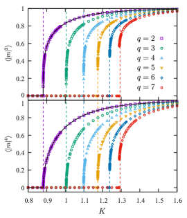
Temperature dependence of the magnetization on the $q$-state Potts model ($q=2,\dots,7$) without the external magnetic field is shown in Fig. 3. Here we perform $40$ steps of HOTRG calculation ($N=2^{40}$) with the bond dimension $\chi=48$. The HOTRG results in the Ising model ($q=2$) are on a curve of the exact result in the thermodynamic limit [27]. Properties of phase transitions will be discussed in the next section.

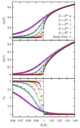
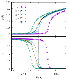
Next, we compare the proposed method with the Monte Carlo (MC) simulations in the Ising model ($q=2$) on small systems (Fig.4). We use the Swendsen-Wang algorithm for the MC simulations [29]. The magnetization, $\langle|m|^{2}\rangle$ and $\langle|m|^{4}\rangle$, agree well with the MC results. However, the Binder ratio shows slight deviation from the MC results because of truncation errors in the renormalization. As shown in Fig. 5, the Binder ratio with the finite bond dimension shows a sharp drop whose location fluctuates around the exact critical temperature and seems to converge to the exact solution in the limit $\chi\rightarrow\infty$. At criticality, the Binder ratio takes a universal value. For the Ising model, $U_{4}=1.167929(1)$ is reported in Ref. [28], while the HOTRG calculation with $\chi=48$ produces $U_{4}=1.1574$ after $30$ renormalization steps ($N=2^{30}$).

Figure 6: The relative error of the estimated transition point $K_{c}(\chi)$ from the exact solution $K_{c}$. The dashed line is proportional to $\chi^{-3.5}$.

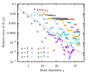
The transition temperature $K_{c}(\chi)$ estimated under the fixed bond dimension $\chi$ is determined by a location of a jump of the Binder ratio. We search a jump point by using the bisection algorithm. We observe that $K_{c}(\chi)$ oscillates around the exact transition temperature and converges to $K_{c}$ in the thermodynamic limit. Plateaus of $K_{c}(\chi)$ for large $q$ are due to degeneracy of the entanglement spectrum. The relative error $\Delta K_{c}\equiv(K_{c}(\chi)-K_{c})/K_{c}$ seems to decrease with $\chi^{-3.5}$ (Fig. 6), which will be discussed later.

4 Finite-size scaling analysis

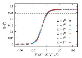
The finite-size scaling (FSS) analysis of the magnetization $\langle|m|^{2}\rangle$ makes clear distinction between discontinuous and continuous phase transitions. In the $5$-state Potts model, the phase transition is weekly first-order and its critical exponent is $1/\nu=d=2$ and $\beta=0$ [30, 31]. The HOTRG result falls on a single curve by using the standard scaling form

$$\langle|m|^{2}\rangle\sim L^{-2\beta/\nu}g(L^{1/\nu}\delta).$$ (28)

with the exact exponents (Fig. 7) where $L$ denotes the system length ($N=L^{2}$). The reduced temperature is defined as $\delta\equiv(K-K_{c}(\chi))/K_{c}$ and we use the estimated critical temperature $K_{c}(\chi)$ already obtained from a jump of the Binder ratio. The plateau of the scaling function in low-temperature region also implies discontinuity of the magnetization at the first-order phase transition point. The plateau height overestimates the magnetization discontinuity at the transition point, whose exact value is known as $\Delta m^{2}_{\text{exact}}=0.24220$ for the $5$-state Potts model [32]. Similar to the estimated transition temperature $K_{c}(\chi)$, we observed that the plateau height depends on the bond dimension and fluctuates around the exact value.

Figure 7: Finite-size scaling plots of the magnetization $\langle|m|^{2}\rangle$ on the 5-state Potts models by HOTRG with $\chi=48$. The critical exponents are fixed to the known values for the first-order transition, that is, $1/\nu=2$ and $\beta=0$. The horizontal dashed line indicates the exact value of spontaneous magnetization at the transition temperature [32].

Figure 8: Finite-size scaling plots of the magnetization $\langle|m|^{2}\rangle$ on the 4-state Potts models by HOTRG with $\chi=48$. We assumed the scaling form Eq. (28) without the logarithmic multiplicative corrections.

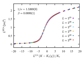
On the other hand, the phase transition of the $4$-state Potts model is continuous. The FSS analysis of the HOTRG result with $\chi=48$ is shown in Fig. 8. The critical exponents are estimated as $1/\nu=1.5369(9)$, $\beta=0.0899(1)$ using the kernel method proposed in Ref. [33]. These values are close to the known exact result $1/\nu=3/2$ and $\beta=1/12=0.0833\cdots$. During the FSS procedure, the critical temperature $K_{c}(\chi)$ is fixed to the value estimated from a jump of the Binder ratio as mentioned before. We need to comment on the fact that the $4$-state Potts model has a marginal operator which yields logarithmic multiplicative corrections [34, 35, 36]. However, since the system size we used for FSS is sufficiently large, significant effect for the logarithmic corrections is not observed. Assuming the scaling form with the logarithmic corrections

$$\langle|m|^{2}\rangle\sim L^{-2\beta/\nu}(\log L)^{1/8}g^{\prime}(L^{1/\nu}(\log L)^{-3/4}t),$$ (29)

we estimate critical exponents as $1/\nu=1.5992(8)$ and $\beta=0.0832(1)$.

A slope of physical quantities at the transition temperature also provides information about critical exponents. Especially the Binder ratio, a dimensionless quantity, satisfies

$$\log\left|\frac{\partial U_{4}}{\partial\delta}\right|_{\delta=0}=c+\frac{1}{\nu}\log L+O(L^{-\omega}),$$ (30)

where $\omega$ is an exponent for correction to scaling. Since we already precisely estimated the transition point with fixed bond dimension from a jump of the Binder ratio, we use a definition $\delta\equiv(K-K_{c}(\chi))/K_{c}$. It is different from the crossing point analysis for the Monte Carlo simulation [37]. The left-hand side of Eq. (30) fits well to a linear line for large system size (Fig. 9(a)). Here, we consider $\log(U_{4}-1)$ instead of $U_{4}$ since it is linear with respect to the inverse temperature around the first-order transition point. (Its phenomenological argument was shown in Ref. [21].) The system size where the data are on a line is smaller than the known correlation length. The correlation length at the transition point approaching from the disordered phase is 2512.2 and 48.1 for $q=5$ and $7$, respectively [38]. In the $5$-state Potts model, a point at $L=512$ is already on the fitting line. This behavior is consistent with the finite-size scaling analysis reported in Ref. [21].

Figure 9: (a) Derivative of $\log(U_{4}-1)$ at the estimated transition point with $\chi=48$. (b) The $\chi$-dependence of the estimated critical exponents $1/\nu$. The dashed horizontal lines indicate the exact values.

Table 1: The critical exponents $1/\nu$ estimated from a slope of the Binder ratio with $\chi=48$. An error indicates the standard error of the fit.

$q$	2	3	4	5	7
Exact	1	$6/5$	$3/2$	2	2
Slope	1.026(2)	1.305(10)	1.544(1)	2.006(2)	2.0001(5)

The estimated critical exponent $1/\nu$ seems to converge to the exact value in the limit $\chi\rightarrow\infty$ (Fig. 9(b)). Large correction to scaling may cause instability in $q=4$ in contrast to FSS of the squared magnetization. In Table 1, we list the critical exponent $1/\nu$ estimated by HOTRG calculations with $\chi=48$. An effect of the finite bond dimension is larger than the standard error of the fit. Our method provides less accurate critical exponent than the CTMRG method [23]. However we would like to emphasize that our analysis does not use any assumptions about the exact transition temperature and the exact energy at criticality, while the CTMRG result used them. Though using the exact values usually increases the accuracy of the estimates drastically, they are not available in general circumstances. The scaling dimensions can also be determined from the eigenvalue of the transfer matrix [39]. However, they are not stable in the HOTRG procedure because of residual short-range correlation as well as TRG [11].

5 Conclusions and Discussions

In this paper, we have proposed an algorithm for the higher-order moments of physical quantities based on the HOTRG method. The systematic summation technique provides the recursion formula for coarse-graining impurity tensors. We have shown that this method calculates the order parameter and the Binder ratio in the Potts model on the square lattice. The transition temperature is precisely determined from a jump of the Binder ratio. Our results are more accurate than the Monte Carlo results. For example, we have achieved $\Delta K_{c}=8.3\times 10^{-6}$ in the 5-state Potts model, while the nonequilibrium relaxation analysis did $2.5\times 10^{-5}$ [20]. The critical exponents are reproduced via FSS analysis. The weakly first-order transition in the $5$-state Potts model is clearly distinct from the continuous transition. This judgment has been made possible by the method proposed in this article. There are two essential points: (i) the advantage in the system size compared to the MC approaches, and (ii) the advantage of symmetry-respecting method over the numerical differentiation approaches.

Our method easily approaches a huge system size which the MC method cannot treat. In the case of no magnetic field, our scheme does not break the spin-rotational symmetry, in other words, each tensor is invariant or covariant under the spin rotation. This fact stabilizes calculations and is an advantage over the numerical differentiation approach because the latter needs to introduce a tiny magnetic field which breaks symmetry. Although we considered the two-dimensional square lattice in this paper, generalization to higher-dimensional systems is straightforward as well as the HOTRG method.

The accuracy of the HOTRG method depends on the bond dimension $\chi$. We observed that the shift of effective critical point roughly scaled as $\Delta K_{c}\sim\chi^{-3.5}$ (Fig. 6). This behavior would relate to the finite-$\chi$ scaling. The effective correlation length satisfies $\xi_{\text{eff}}\sim\chi^{\kappa}$ and the argument of the entanglement entropy based on the conformal invariance provides

$$\kappa=\frac{6}{c\left(\sqrt{12/c}+1\right)},$$ (31)

where $c$ is the central charge. For the Ising model ($c=1/2$), three-state ($c=4/5$) and four-state ($c=1$) Potts models, we have $\kappa=2.034$, $1.539$, and $1.334$, respectively. On the other hand, the scaling of the effective correlation length implies $\Delta K_{c}\sim\chi^{-\kappa/\nu}$. However, our observation is inconsistent with this behavior. It indicates that the naive scaling relation for $\Delta K_{c}$ needs to be correct, which remains as a future issue.

Lastly, we would like to mention possibilities of further improvements in the present method. One is an introduction of the environment tensor. The higher-order second renormalization group method successes to significantly improve the accuracy by globally optimizing the truncation scheme [9]. The other is entanglement filtering [39]. It is known that HOTRG does not remove short-range entanglement completely and eventually gets stuck into a fictitious fixed point [40]. Entanglement filtering techniques, such as a loop-TNR approach [11], a graph independent local truncation’s (GILT) [41], and a full environment truncation (FET) [42], can filter out internal entanglement. Recently entanglement branching was proposed as another approach to manage flow of entanglement [43]. Thus a combination of HOTRG with these techniques will catch the true critical phenomena, which will be considered in future works.

References

- [1] J. I. Cirac, F. Verstraete, Renormalization and tensor product states in spin chains and lattices, J. Phys. A: Math. Theor. 42 (50) (2009) 504004. doi:10.1088/1751-8113/42/50/504004.
- [2] R. Orús, A practical introduction to tensor networks: Matrix product states and projected entangled pair states, Ann. Phys. 349 (2014) 117–158. doi:10.1016/j.aop.2014.06.013.
- [3] S. R. White, Density matrix formulation for quantum renormalization groups, Phys. Rev. Lett. 69 (1992) 2863–2866. doi:10.1103/PhysRevLett.69.2863.
- [4] F. Verstraete, J. I. Cirac, Renormalization algorithms for quantum-many body systems in two and higher dimensions (2004). arXiv:cond-mat/0407066.
- [5] Z. Y. Xie, J. Chen, J. F. Yu, X. Kong, B. Normand, T. Xiang, Tensor renormalization of quantum many-body systems using projected entangled simplex states, Phys. Rev. X 4 (2014) 011025. doi:10.1103/PhysRevX.4.011025.
- [6] M. Levin, C. P. Nave, Tensor renormalization group approach to two-dimensional classical lattice models, Phys. Rev. Lett. 99 (2007) 120601. doi:10.1103/PhysRevLett.99.120601.
- [7] Z. Y. Xie, H. C. Jiang, Q. N. Chen, Z. Y. Weng, T. Xiang, Second renormalization of tensor-network states, Phys. Rev. Lett. 103 (2009) 160601. doi:10.1103/PhysRevLett.103.160601.
- [8] H. H. Zhao, Z. Y. Xie, Q. N. Chen, Z. C. Wei, J. W. Cai, T. Xiang, Renormalization of tensor-network states, Phys. Rev. B 81 (2010) 174411. doi:10.1103/PhysRevB.81.174411.
- [9] Z. Y. Xie, J. Chen, M. P. Qin, J. W. Zhu, L. P. Yang, T. Xiang, Coarse-graining renormalization by higher-order singular value decomposition, Phys. Rev. B 86 (2012) 045139. doi:10.1103/PhysRevB.86.045139.
- [10] G. Evenbly, G. Vidal, Tensor network renormalization, Phys. Rev. Lett. 115 (2015) 180405. doi:10.1103/PhysRevLett.115.180405.
- [11] S. Yang, Z.-C. Gu, X.-G. Wen, Loop optimization for tensor network renormalization, Phys. Rev. Lett. 118 (2017) 110504. doi:10.1103/PhysRevLett.118.110504.
- [12] W. Shun, X. Zhi-Yuan, C. Jing, B. Normand, X. Tao, Phase transitions of ferromagnetic potts models on the simple cubic lattice, Chin. Phys. Lett. 31 (7) (2014) 070503. doi:10.1088/0256-307X/31/7/070503.
- [13] R. J. Baxter, Exactly Solved Models in Statistical Mechanics, Academic Press, London, 1982.
- [14] K. Binder, Finite size scaling analysis of ising model block distribution functions, Z. Phys. B 43 (2) (1981) 119–140. doi:10.1007/BF01293604.
- [15] C. G. West, A. Garcia-Saez, T.-C. Wei, Efficient evaluation of high-order moments and cumulants in tensor network states, Phys. Rev. B 92 (2015) 115103. doi:10.1103/PhysRevB.92.115103.
- [16] Y.-P. Lin, Y.-J. Kao, P. Chen, Y.-C. Lin, Griffiths singularities in the random quantum ising antiferromagnet: A tree tensor network renormalization group study, Phys. Rev. B 96 (2017) 064427. doi:10.1103/PhysRevB.96.064427.
- [17] P. Corboz, Variational optimization with infinite projected entangled-pair states, Phys. Rev. B 94 (2016) 035133. doi:10.1103/PhysRevB.94.035133.
- [18] R. B. Potts, Some generalized order-disorder transformations, Math. Proc. Camb. Phil. Soc. 48 (1) (1952) 106–109. doi:10.1017/S0305004100027419.
- [19] F. Y. Wu, The potts model, Rev. Mod. Phys. 54 (1982) 235–268. doi:10.1103/RevModPhys.54.235.
- [20] Y. Ozeki, K. Kasono, N. Ito, S. Miyashita, Nonequilibrium relaxation analysis for first-order phase transitions, Physica A 321 (1) (2003) 271 – 279. doi:10.1016/S0378-4371(02)01788-0.
- [21] S. Iino, S. Morita, A. W. Sandvik, N. Kawashima, Detecting signals of weakly first-order phase transitions in two-dimensional potts models (2018). arXiv:1801.02786.
- [22] T. Nishino, K. Okunishi, Corner transfer matrix renormalization group method, J. Phys. Soc. Jpn. 65 (4) (1996) 891–894. doi:10.1143/JPSJ.65.891.
- [23] T. Nishino, K. Okunishi, Corner Transfer Matrix Algorithm for Classical Renormalization Group, J. Phys. Soc. Japan 66 (10) (1997) 3040–3047. doi:10.1143/JPSJ.66.3040.
- [24] T. Nishino, K. Okunishi, Numerical Latent Heat Observation of the Potts Model, J. Phys. Soc. Japan 67 (4) (1998) 1492–1493. doi:10.1143/JPSJ.67.1492.
- [25] S. Singh, R. N. C. Pfeifer, G. Vidal, Tensor network decompositions in the presence of a global symmetry, Phys. Rev. A 82 (2010) 050301. doi:10.1103/PhysRevA.82.050301.
- [26] S. Singh, R. N. C. Pfeifer, G. Vidal, Tensor network states and algorithms in the presence of a global u(1) symmetry, Phys. Rev. B 83 (2011) 115125. doi:10.1103/PhysRevB.83.115125.
- [27] C. N. Yang, The spontaneous magnetization of a two-dimensional ising model, Phys. Rev. 85 (1952) 808–816. doi:10.1103/PhysRev.85.808.
- [28] G. Kamieniarz, H. W. J. Blote, Universal ratio of magnetization moments in two-dimensional ising models, J. Phys. A: Math. Gen. 26 (2) (1993) 201. doi:10.1088/0305-4470/26/2/009.
- [29] R. H. Swendsen, J.-S. Wang, Nonuniversal critical dynamics in monte carlo simulations, Phys. Rev. Lett. 58 (2) (1987) 86–88. doi:10.1103/PhysRevLett.58.86.
- [30] B. Nienhuis, M. Nauenberg, First-Order Phase Transitions in Renormalization-Group Theory, Phys. Rev. Lett. 35 (8) (1975) 477–479. doi:10.1103/PhysRevLett.35.477.
- [31] M. E. Fisher, A. N. Berker, Scaling for first-order phase transitions in thermodynamic and finite systems, Phys. Rev. B 26 (5) (1982) 2507–2513. doi:10.1103/PhysRevB.26.2507.
- [32] R. J. Baxter, Magnetisation discontinuity of the two-dimensional potts model, J. Phys. A: Math. Gen. 15 (10) (1982) 3329. doi:10.1088/0305-4470/15/10/035.
- [33] K. Harada, Bayesian inference in the scaling analysis of critical phenomena, Phys. Rev. E 84 (2011) 056704. doi:10.1103/PhysRevE.84.056704.
- [34] M. Nauenberg, D. J. Scalapino, Singularities and scaling functions at the potts-model multicritical point, Phys. Rev. Lett. 44 (1980) 837–840. doi:10.1103/PhysRevLett.44.837.
- [35] J. L. Cardy, M. Nauenberg, D. J. Scalapino, Scaling theory of the potts-model multicritical point, Phys. Rev. B 22 (1980) 2560–2568. doi:10.1103/PhysRevB.22.2560.
- [36] J. Salas, A. D. Sokal, Logarithmic corrections and finite-size scaling in the two-dimensional 4-state potts model, J. Stat. Phys. 88 (3) (1997) 567–615. doi:10.1023/B:JOSS.0000015164.98296.85.
- [37] H. Shao, W. Guo, A. W. Sandvik, Quantum criticality with two length scales, Science 352 (6282) (2016) 213–216. doi:10.1126/science.aad5007.
- [38] E. Buddenoir, S. Wallon, The correlation length of the potts model at the first-order transition point, J. Phys. A: Math. Gen. 26 (13) (1993) 3045. doi:10.1088/0305-4470/26/13/009.
- [39] Z.-C. Gu, X.-G. Wen, Tensor-entanglement-filtering renormalization approach and symmetry-protected topological order, Phys. Rev. B 80 (2009) 155131. doi:10.1103/PhysRevB.80.155131.
- [40] H. Ueda, K. Okunishi, T. Nishino, Doubling of entanglement spectrum in tensor renormalization group, Phys. Rev. B 89 (2014) 075116. doi:10.1103/PhysRevB.89.075116.
- [41] M. Hauru, C. Delcamp, S. Mizera, Renormalization of tensor networks using graph-independent local truncations, Phys. Rev. B 97 (2018) 045111. doi:10.1103/PhysRevB.97.045111.
- [42] G. Evenbly, Gauge fixing, canonical forms, and optimal truncations in tensor networks with closed loops, Phys. Rev. B 98 (2018) 085155. doi:10.1103/PhysRevB.98.085155.
- [43] K. Harada, Entanglement branching operator, Phys. Rev. B 97 (2018) 045124. doi:10.1103/PhysRevB.97.045124.