Elastic Scattering in General Relativistic Ray Tracing for Neutrinos

Abstract

We present a covariant ray tracing algorithm for computing high-resolution neutrino distributions in general relativistic numerical spacetimes with hydrodynamical sources. Our formulation treats the very important effect of elastic scattering of neutrinos off of nuclei and nucleons (changing the neutrino’s direction but not energy) by incorporating estimates of the background neutrino fields. Background fields provide information about the spectra and intensities of the neutrinos scattered into each ray. These background fields may be taken from a low-order moment simulation or be ignored, in which case the method reduces to a standard state-of-the-art ray tracing formulation. The method handles radiation in regimes spanning optically thick to optically thin. We test the new code, highlight its strengths and weaknesses, and apply it to a simulation of a neutron star merger to compute neutrino fluxes and spectra, and to demonstrate a neutrino flavor oscillation calculation. In that environment, we find qualitatively different fluxes, spectra, and oscillation behaviors when elastic scattering is included.

I Introduction

Neutrinos are one of the dominant energy transport phenomena at play in neutron star mergers: heating, cooling, and pushing the disrupted nuclear matter. In addition, they change the composition of the matter via charged current interactions. Because neutrinos scatter over length scales both large and small with respect to fluid scales, accurate models require a neutrino treatment that respects the freedom of neutrino distribution functions to vary drastically from geometrically simple distributions in thermodynamic equilibrium.

This is a challenging task in the environment of a merger, which generally lacks any spatial symmetries, so that fully general solutions to the Boltzmann Equation are not feasible. Leakage approximations (Ruffert et al., 1996; Rosswog and Liebendörfer, 2003; Deaton et al., 2013; Galeazzi et al., 2013; Perego et al., 2016; Radice et al., 2016) capture some of the qualitative effects of neutrinos on the matter, but provide extremely limited information about the neutrino field itself. Monte Carlo methods like those used in supernova simulations Abdikamalov et al. (2012) and stationary models of accretion disks Richers et al. (2015) are an excellent tool but require large computational resources because of the need to use a large number of particles to fully and precisely sample the high dimensional parameter space (seven-dimensional in the general case).

The state of the art today for neutron star merger calculations couples radiation and matter using a truncated moment formalism (Foucart et al., 2015, 2016a), evolving the zeroth- and first-angular moments of the energy density, that is the total energy- and momentum-densities. This method, commonly called M1 transport, was formulated by Thorne (1981) and modernized by Shibata et al. (2011). M1 transport has recently become popular in the core-collapse supernova community as well Kuroda et al. (2012); Just et al. (2015); O’Connor (2015); Skinner et al. (2016); Roberts et al. (2016).

For merger simulations, Foucart et al. (2016b) have recently expanded their M1 transport code to also evolve the zeroth-angular moment of the number density, providing total energy densities and average energies throughout the simulated volume. Even so, with M1 transport codes only evolving two angular moments and one or two energy moments, they can extract only limited angular and spectral information from the neutrino fields.

But many interesting unsolved problems require an accurate model of the neutrino spectra and angular distributions. With a model of the neutrino emission from a merger we can 1) examine neutrino effects on the nucleosynthesis of the ejected material (Surman et al., 2011; Roberts et al., 2017), 2) explore the rich flavor oscillation physics likely to occur (Malkus et al., 2012, 2014, 2016; Zhu et al., 2016; Väänänen and McLaughlin, 2016), 3) improve closure relations used in M1 transport schemes (Rampp and Janka, 2002; Shibata et al., 2011; Cardall et al., 2013; Foucart et al., 2015; O’Connor, 2015), and 4) study possible jet formation due to neutrino annihilation (Ruffert and Janka, 1999; Asano and Fukuyama, 2000; Birkl et al., 2007; Harikae et al., 2010; Zalamea and Beloborodov, 2011; Leng and Giannios, 2014; Just et al., 2016).

Angular and spectral neutrino distributions in neutron star merger simulations have just recently become available with a coupled Monte-Carlo-M1 scheme (Foucart, 2018; Foucart et al., 2018). In this work, however, we present a ray tracing method to compute neutrino distribution functions from the more widely available state-of-the-art general relativistic M1 transport hydrodynamics simulations. We choose ray tracing because it is conceptually simple, numerically inexpensive, and extends to high resolution in energy and angle by simply increasing the number of rays sampled. Furthermore, the computational implementation parallellizes trivially.

With a ray tracing method we approach radiation transport from the perspective of a single observer at a spacetime event $x_{o}^{\alpha}$. Our goal is to compute the distribution function $f^{\nu_{\sigma}}(x_{o}^{\alpha};p_{\beta})$, or the amount of neutrino radiation of species $\nu_{\sigma}\in\{\nu_{e},\nu_{\mu},\nu_{\tau},\bar{\nu}_{e},\bar{\nu}_{\mu},\bar{\nu}_{\tau}\}$ with momentum $p_{\beta}$ impinging on $x_{o}^{\alpha}$. To do so we trace a geodesic trajectory from $x_{o}^{\alpha}$ in the backwards direction $-p_{\beta}$ to sample the incoming radiation along that line of sight. By tracing a family of rays intersecting $x_{o}^{\alpha}$ we build up a picture of the distribution function there. And by sampling many observation points we construct a global picture of $f^{\nu_{\sigma}}(x^{\alpha};p_{\beta})$.

The ray tracing framework is conceptually simple because it solves the equation of radiation transport (Eqn. 8) along characteristics, reducing it to a one-dimensional ordinary differential equation. It is numerically cheap because it confines computations of $f^{\nu_{\sigma}}(x_{o}^{\alpha};p_{\beta})$ to the past light-cone of $x_{o}^{\alpha}$, with the history of that light-cone truncated at large optical depth. It easily extends to high resolution in energy and angle by simply increasing the number of rays sampled. And it parallelizes trivially by ray, since each ray is computed independently.

Several ray tracing formulations for radiation transport already exist. Most formulations assume an analytic spacetime metric (Birkl et al., 2007; Caballero et al., 2009; Harikae et al., 2010; Kovács and Harko, 2011). And many make the simplifying assumption of blackbody emission from a neutrinosurface (Birkl et al., 2007; Caballero et al., 2009; Kovács and Harko, 2011), limiting them to equilibrium, optically-thick configurations. Current state-of-the-art ray tracing formulations avoid the assumption of blackbody spectra by integrating a local emissivity along each geodesic (e.g. Harikae et al. (2010) for neutrinos and Younsi et al. (2012) for photons). But no formulations to date account for the important scattering and pair processes outlined in Tab. 1. We build upon these existing ray tracing formulations by eschewing any assumptions about the spacetime geometry, integrating local emissivities, and including elastic scattering in the integration along each geodesic.

We formulate the ray tracing equations covariantly—free from assumptions about the spacetime geometry or coordinates. This is essential because we want to apply the method as a postprocessing step using time snapshots of data computed from time-dependent general relativistic evolutions. The spacetime represented in these snapshots is not analytic (i.e. Kerr). And even in configurations that are described well by the Kerr metric (e.g. a low-mass disk around a massive black hole), the evolution coordinates are unlikely to present the metric in a familiar analytic form. This is because integrating the Einstein Equations often requires complicated, time-dependent gauge conditions (Lindblom et al., 2006; Foucart et al., 2013).

Elastic scattering (see Tab. 1) can signicantly modify neutrino distributions in angle and dilute the emitted spectrum over a larger emitting surface (Perego et al., 2016). This is especially pronounced in the case of heavy-lepton neutrinos. Inelastic scattering and pair processes can introduce further modifications. Any phenomena that involve neutrino-neutrino interactions, for example neutrino oscillations Duan et al. (2010); Malkus et al. (2012); Vlasenko and McLaughlin (2018) and neutrino-antineutrino annihilation Asano and Fukuyama (2000), depend sensitively on the angular distribution. And spectral changes in neutrino distributions can strongly affect the nuclear processes occuring in the ejected and irradiated material Surman et al. (2006); Malkus et al. (2012); Caballero et al. (2012); Foucart et al. (2016b). The ray tracing method we present in this paper captures the dominant effects of elastic scattering, while leaving the physics of inelastic scattering and pair processes for later work.

Table 1: We analyze neutrino interaction processes in terms of these categories. $\nu$ without a label represents a neutrino or antineutrino of any flavor, $N$ represents a nucleon $n$ or $p$, ${}^{Z}A$ represents a nucleus with mass number $A$ and charge $Z$, and $\gamma$ represents a high-energy photon. A prime indicates a change in that particle’s energy.

absorption/emission	$\nu_{e}+n\leftrightarrow e^{-}+p$
	$\bar{\nu}_{e}+p\leftrightarrow e^{+}+n$
	$\nu_{e}+{}^{A}Z\leftrightarrow e^{-}+{}^{A}(Z+1)$
elastic scattering	$\nu+N\leftrightarrow\nu+N$
	$\nu+{}^{A}Z\leftrightarrow\nu+{}^{A}Z$
inelastic scattering	$\nu+e^{-}\leftrightarrow\nu^{\prime}+e^{-^{\prime}}$
	$\nu+e^{+}\leftrightarrow\nu^{\prime}+e^{+^{\prime}}$
thermal pair processes	$\nu+\bar{\nu}\leftrightarrow e^{-}+e^{+}$
	$\nu+\bar{\nu}+N+N\leftrightarrow N^{\prime}+N^{\prime}$
	$\nu+\bar{\nu}\leftrightarrow\gamma$

Ray tracing is ideally suited to problems requiring detailed knowledge of radiation distribution functions over small regions of spacetime: for example along a matter or radiation trajectory, or over a small volume outside a source. Furthermore, our method is time-dependent, allowing us to compute radiation fields in dynamical systems. But it is formulated as a post-processing step, with the ray tracing computated on volume data saved in several steps of the fluid evolution. Thus for dynamical systems the memory demands can be prohibitively large.

More fundamentally, though, ray tracing is limited by its naive treatment of the Boltzmann Equation (Eqn. 8), a treatment which essentially decouples different neutrino momenta and species. When solving for $f^{\nu_{\sigma}}(x^{\alpha};p_{\beta})$, we have no information about the distribution at different momenta $f^{\nu_{\sigma}}(x^{\alpha};p^{\prime}_{\beta})$, or about the distribution of the relevant antineutrino species $f^{\bar{\nu}_{\sigma}}(x^{\alpha};p^{\prime}_{\beta})$; these missing data are essential ingredients for the source terms of the Boltzmann Equation describing the creation and destruction of neutrinos due to the interaction processes described in Tab. 1.

In this paper we outwit this limitation by incorporating coupled source terms that depend on either previously-evolved or analytical estimates of the neutrino fields. To incorporate scattering processes in our method, we employ estimates of the lowest-order moment of the neutrino distribution function computed in an M1 transport simulation. If moments are not available either from an M1 transport evolution or a trustworthy analytical estimate, we may drop the coupling terms and our method reduces to the current state-of-the-art ray tracing methods neglecting scattering. Our method is not a standalone radiation transport scheme, but serves as the final component of a hybrid scheme, piggy-backing on a lower-order radiation transport method as a post-processing step.

In Sec. II we derive the ray tracing equations from the Boltzmann Equation and describe our numerical scheme. In Sec. III we present tests of the code. In Sec. IV we present neutrino fields in the dynamical environment following the merger of two neutron stars, and compute neutrino flavor oscillation along an outgoing ray, including the effects of coherent forward scattering with ambient neutrinos. In Sec. V we summarize our work and anticipate improvements.

Greek tensor indices ($\alpha,\beta,...$) range over all four coordinates, whereas Latin indices ($i,j,...$) range over the spatial coordinates 1–3, or over a more general set, e.g. the set of all elastic scattering interactions. We use naturalized units in which $\{\hbar,c,k_{\rm B}\}=1$. And for most of the remainder of this article we suppress neutrino species label $\nu_{\sigma}$ since the formulation is general to any species. Where we do reference particular species we use the three categories relevant to the energy scales of mergers, $\nu_{e}$, $\bar{\nu}_{e}$, and $\nu_{x}=\left\{\nu_{\mu},\bar{\nu}_{\mu},\nu_{\tau},\bar{\nu}_{\tau}\right\}$.

II Ray tracing formulation

The neutrino distribution function, $f(x^{\alpha};p_{\beta})$ is an invariant quantity counting the number of neutrinos in a given six-volume of phase space centered on $(x^{\alpha},p_{\beta})$. The phase space volume elements are defined with respect to a fiducial observer passing through event $x^{\alpha}$ with velocity $u^{\alpha}$:

$$dV \equiv\sqrt{-\psi}\,dx\,dy\,dz\,u^{t}$$ (1)

$$dP \equiv\frac{1}{\sqrt{-\psi}}\,dp_{x}\,dp_{y}\,dp_{z}\,\frac{\varepsilon}{p^{t}},$$ (2)

where $\psi$ represents the determinant of the spacetime metric, the index $t$ indicates the time-component of the given four-vector, and

$$\varepsilon\equiv-p_{\mu}u^{\mu}$$ (3)

is the neutrino energy measured by our observer. The number of particles in a given six-volume is

$$dN=\frac{g}{(2\pi)^{3}}\,f\,dV\,dP,$$ (4)

where $g$ counts the number of spin states accessible to the particles ($g=1$ for neutrinos), and $f$ is the distribution function. Each of $dV$, $dP$, $dN$, and $f$ are spacetime invariants (Debbasch and van Leeuwen, 2009a, b; Lindquist, 1966).

We may decompose the neutrino momentum like

$$p_{\beta}=\varepsilon(u_{\beta}+\ell_{\beta}),$$ (5)

with $\ell_{\beta}$ the direction normal subject to the constraints $u^{\alpha}\ell_{\alpha}=0$ and $\ell^{\alpha}\ell_{\alpha}=1$. With this decompositon we can write the arguments to the distribution function $f(x^{\alpha};\varepsilon,\ell_{\beta})$.

Because $\ell_{\beta}$ is subject to two constraints (normalization and orthogonality to the observer’s velocity) it has only two remaining degrees of freedom; we make this explicit by defining its spatial cartesian components with respect to spherical polar angles

$$\ell_{\alpha}\rightarrow q(s,\sin a\cos b,\sin a\sin b,\cos a),$$ (6)

with $q$ and $s$ functions of $a$ and $b$. Now our symbol for the distribution function, $f(x^{\alpha};\varepsilon,a,b)$, makes manifest its seven independent arguments.

We also define a rotated frame

$$\ell_{\alpha^{\prime}}=\frac{\partial x^{\alpha}}{\partial x^{\alpha^{\prime}}}\,\ell_{\alpha}$$

in which the cartesian components of the direction 1-form are defined

$$\ell_{\alpha^{\prime}}\rightarrow q(s,\sin A\cos B,\sin A\sin B,\cos A),$$ (7)

so that momenta with vanishing polar angle $A$ move outward along coordinate radial rays. This transformation is chosen so that for an observer far from the source, incoming radiation will be concentrated into a narrow beam around $\cos A\approx 1$, independent of that observer’s position in coordinate space. For explicit definitions see App. A.

In Minkowski spacetime, and for a stationary observer $u_{\beta}\rightarrow(-1,0,0,0)$, we would have $s=0$, $q=1$, and $\varepsilon=-p_{t}$. In that case $\cos A$ may be identified with the familiar forward direction cosine $\mu$ (Shu, 1991; Mihalas and Weibel-Mihalas, 1999).

II.1 Boltzmann Equation

In the limit of large oscillation lengths (see Sec. IV.2), neutrino radiation obeys the relativistic Boltzmann Equation, which, suppressing the arguments of $f$ for simplicity, is written,

$$\frac{d}{d\lambda}f=C[f],$$ (8)

where $d/d\lambda$ denotes a derivative with respect to the affine parameter defining the neutrino momentum (Eqn. 20 below) and $C[f]$ is the source term arising from interactions with the medium. As we will show below in Eqn. 23, the affine parameter has dimension ${\rm length}\,{\rm energy}^{-1}$, so the source term has dimension ${\rm energy}\,{\rm length}^{-1}$. The source term varies over phase space $(x^{\alpha},p_{\beta})$, and depends locally on the distribution function $f$ and nonlocally on the distribution function of this neutrino and its antiparticle at different momenta, $f^{\prime}$ and $\bar{f}^{\prime}$. For simplicity we symbolize all of these dependencies with the shorthand $C[f]$. The various neutrino interactions contributing to $C[f]$ are detailed in App. B.

We make the right hand side of Eqn. 8 explicit by writing the source term linear in $f$:

$$\frac{d}{d\lambda}f =\mathscr{E}-\mathscr{K}f$$ (9)

$$=\mathscr{K}(\mathscr{S}-f)$$ (10)

where we have introduced $\mathscr{E}$, the invariant total emissivity, and $\mathscr{K}$, the invariant total opacity. These describe respectively the energy gained and the energy lost per length traveled by the neutrino, true scalar quantities which take identical values for all observers. In the second form we have introduced the source function $\mathscr{S}\equiv\mathscr{E}/\mathscr{K}$, which makes manifest the behavior of the right hand side, driving $f$ toward $\mathscr{S}$ over a lengthscale $\mathscr{K}^{-1}$ in the affine parameter; or from Eqn. 23 below, over a proper lengthscale $\varepsilon/\mathscr{K}$ measured by the fiducial observer.

These coefficients are computed by considering their dependence on neutrino and antineutrino distribution functions at other momenta (i.e. Fermi-blocking). We consider the two dominant classes of interactions in this work: the absorption/emission (AE) and elastic scattering (SE) processes listed in Tab. 1; note that we also include the important thermal pair processes (PP) for heavy-lepton neutrinos by incorporating an approximate pair emissivity into their absorption/emission coefficients; see App. B for details. Thus we separate these coefficients:

$$\mathscr{E} =\mathscr{E}_{\rm AE}+\mathscr{E}_{\rm SE},$$ (11)

$$\mathscr{K} =\mathscr{K}_{\rm AE}+\mathscr{K}_{\rm SE}.$$ (12)

The absorption/emission coefficients are computed from sums over the relevant emissivities and opacities for the reactions

$$\nu_{e}+n \leftrightarrow e^{-}+p,$$

$$\bar{\nu}_{e}+p \leftrightarrow e^{+}+n,$$

$$\nu_{e}+{}^{A}Z \leftrightarrow e^{-}+{}^{A}(Z+1),$$

with ${}^{A}Z$ representing a nucleus of mass number $A$ and charge $Z$. In terms of the emissivity $j(\varepsilon)$ describing number of neutrinos of energy $\varepsilon$ emitted per length, and the absorption opacity $\chi_{a}(\varepsilon)$ describing the number absorbed per length, the coefficients are

$$\mathscr{E}_{\rm AE}(\varepsilon) =\varepsilon\sum_{i\,{\rm reactions}}j_{i}(\varepsilon),$$ (13)

$$\mathscr{K}_{\rm AE}(\varepsilon) =\frac{1}{1-f^{\rm eq}(\varepsilon)}\,\varepsilon\sum_{i\,{\rm reactions}}\chi_{{\rm a},i}(\varepsilon),$$ (14)

where $f^{\rm eq}$ is the distribution function of neutrinos in radiative equilibrium with the matter, i.e. the Fermi-Dirac distribution function

$$f^{\rm eq}(\varepsilon)\equiv\left(1+e^{\varepsilon/(k_{\rm B}T)-\eta_{\nu}}\right)^{-1},$$ (15)

with the neutrino chemical potentials dependent on the local density, temperature, and composition of the fluid via the neutron, proton, and electron chemical potentials: $\eta_{\nu_{e}}=-\eta_{\bar{\nu}_{e}}=\eta_{p}-\eta_{n}+\eta_{e^{-}}$ and $\eta_{\nu_{x}}=0$. The appearance of $f^{\rm eq}$ in Eqn. 14 is due to the Fermionic nature of the neutrinos, causing $\mathscr{K}_{\rm AE}$ to be different than the simple absorption opacity, a phenomenon called stimulated absorption Burrows et al. (2006). By detailed balance of the absorption/emission reactions, we may alternatively write the emissivity in terms of the equilibrium distribution function:

$$\mathscr{E}_{\rm AE}(\varepsilon)=\mathscr{K}_{\rm AE}(\varepsilon)f^{\rm eq}(\varepsilon).$$ (16)

Note that the stimulated absorption coefficient $\mathscr{K}_{\rm AE}$ is identical to the coefficient $\kappa^{*}$ defined in Harikae et al. (2010). See App. B.1 for details.

The elastic scattering coefficients are computed from a background field, and a sum over opacities for the reactions

$$\nu+N \leftrightarrow\nu+N,$$

$$\nu+{}^{A}Z \leftrightarrow\nu+{}^{A}Z,$$

with $N$ standing in for either $n$ or $p$. In terms of a background field $\Phi(\varepsilon)$ describing the number of neutrinos of energy $\varepsilon$ present at this event, and the scattering opacity $\chi(\varepsilon)$ describing the number scattered to other directions per length, the coefficients are

$$\mathscr{E}_{\rm SE}(\varepsilon) =\mathscr{K}_{\rm SE}(\varepsilon)\,\Phi(\varepsilon)\,$$ (17)

$$\mathscr{K}_{\rm SE}(\varepsilon) =\varepsilon\sum_{i\,{\rm reactions}}\chi_{{\rm s},i}(\varepsilon).$$ (18)

In the isotropic limit of trapped radiation, $\Phi$ is equivalent to $f^{\rm eq}$; in the free-streaming limit at a distance $r$ from a source, $\Phi$ attenuates as $r^{-2}$. See App. B.2 for details.

With these definitions we write a separated form of Eqn. 10:

$$\frac{d}{d\lambda}f=\mathscr{K}_{\rm AE}(f^{\rm eq}-f)+\mathscr{K}_{\rm SE}(\Phi-f)$$ (19)

From Eqn. 19 we see that absorption/emission interactions drive the distribution function toward $f^{\rm eq}$ over an affine lengthscale $\mathscr{K}_{\rm AE}^{-1}$, and elastic scattering interactions drive it toward $\Phi$ over an affine lengthscale $\mathscr{K}_{\rm SE}^{-1}$. (Eqn. 23 translates affine length to proper length for a given observer; in this case the proper length scale is $\varepsilon/\mathscr{K}$.)

This paper introduces the use of neutrino densities and fluxes evolved in an M1 transport simulation to estimate the background field, $\Phi$. App. B.2 details a method to calculate $\Phi(\varepsilon)$ in two different ways:

• the spectral method using densities and fluxes extracted from a simulation evolved over multiple energy groups to compute the background field with Eqn. 102,

• the gray method using energy-integrated densities and fluxes extracted from a gray simulation and approximating the energy distribution with Eqns. 110 and 111.

II.2 Trajectories

Each trajectory is uniquely labeled by a pair of vectors giving an event on the trajectory, $x^{\alpha}$, and the momentum at that event, $p_{\beta}$. To designate a family of intersecting trajectories, we keep constant either the emission event $x^{\alpha}_{e}$ or the observation event $x^{\alpha}_{o}$.

Neutrino trajectories obey the geodesic equation, which may be decomposed into the coupled first-order equations

$$\frac{dx^{\alpha}}{d\lambda}=p^{\alpha},$$ (20)

and

$$\frac{dp_{\beta}}{d\lambda}=-\Gamma^{\alpha}_{\beta\gamma}p^{\gamma}p_{\alpha},$$ (21)

where $p^{\alpha}=\psi^{\alpha\beta}p_{\beta}$, $\psi^{\alpha\beta}$ is the inverse of the spacetime metric $\psi_{\alpha\beta}$, and $\Gamma^{\alpha}_{\beta\gamma}$ are the standard connection coefficients,

$$\Gamma^{\alpha}_{\beta\gamma}=\frac{1}{2}\psi^{\alpha\mu}(\psi_{\mu\beta,\gamma}+\psi_{\mu\gamma,\beta}-\psi_{\beta\gamma,\mu}),$$ (22)

with the comma denoting a partial derivative $\psi_{\mu\beta,\gamma}=\partial_{\gamma}\,\psi_{\mu\beta}$.

Each trajectory is parameterized by affine parameter, $\lambda$, increasing in the direction of $\ell_{\beta}$. We label $\lambda=\lambda_{e}$ at $x^{\alpha}_{e}$, as in Fig. 1. If we multiply Eqn. 20 by $u_{\alpha}\equiv dx_{\alpha}/ds$, we find the element of proper distance traversed by the neutrino as measured by the fiducial observer $u^{\alpha}$ is

$$ds=\varepsilon\,d\lambda.$$ (23)

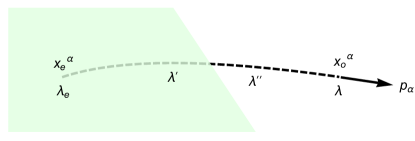
Figure 1: Affine parameterization of a neutrino trajectory of momentum $p_{\alpha}$. The fiducial observer with velocity $u^{\alpha}$ sits at $x^{\alpha}_{o}$, the neutrino emission event is at $x^{\alpha}_{e}$. The affine parameter increases from the emission event: $\lambda_{e}<\lambda^{\prime}<\lambda^{\prime\prime}$. The green slab represents dense matter.

II.3 The Formal Solution

We can integrate Eqn. 19 directly, with the solution split into a boundary, absorption/emission, and a scattering term, $f=f_{\rm bdry}+f_{\rm AE}+f_{\rm SE}$:

$$f_{\rm bdry}(\lambda,\lambda_{e}) =f(\lambda_{e})e^{-\tau(\lambda,\lambda_{e})},$$ (24)

$$f_{\rm AE}(\lambda,\lambda_{e}) =\int_{\lambda_{e}}^{\lambda}d\lambda^{\prime}\,e^{-\tau(\lambda,\lambda^{\prime})}\mathscr{K}_{\rm AE}(\lambda^{\prime})f^{\rm eq}(\lambda^{\prime}),$$ (25)

$$f_{\rm SE}(\lambda,\lambda_{e}) =\int_{\lambda_{e}}^{\lambda}d\lambda^{\prime}\,e^{-\tau(\lambda,\lambda^{\prime})}\mathscr{K}_{\rm SE}(\lambda^{\prime})\Phi(\lambda^{\prime}),$$ (26)

where the optical depth is defined,

$$\tau(\lambda,\lambda^{\prime})\equiv\int_{\lambda^{\prime}}^{\lambda}d\lambda^{\prime\prime}\,\mathscr{K}(\lambda^{\prime\prime}),$$ (27)

and the parameterization conventions are depicted in Fig. 1. Note that Eqn. 27 employs the total absorption plus scattering opacity, so that the optical depth attenuating the integrands of Eqns. 25 and 26 is the total optical depth.

II.4 Moments of the Distribution Function

We may take angular moments of the distribution function:

$$J(\varepsilon) =\frac{\varepsilon^{3}}{(2\pi)^{3}}\oint d\Omega^{\prime}f(\varepsilon,\ell^{\prime}_{\beta})$$ (28)

$$H^{\mu}(\varepsilon) =\frac{\varepsilon^{3}}{(2\pi)^{3}}\oint d\Omega^{\prime}f(\varepsilon,\ell^{\prime}_{\beta})\ell^{\prime\mu}$$ (29)

$$S^{\mu\gamma}(\varepsilon) =\frac{\varepsilon^{3}}{(2\pi)^{3}}\oint d\Omega^{\prime}f(\varepsilon,\ell^{\prime}_{\beta})\ell^{\prime\mu}\ell^{\prime\gamma},$$ (30)

defining the specific energy density, specific momentum density, and specific radiation pressure tensor, respectively. Here “specific” refers to the quantity being integrable over neutrino energy. Integrals 28–30 are performed over a solid angle in momentum space while holding $\varepsilon$ constant: $d\Omega\equiv d(\cos a)\,db$. We also make use of the specific number density and specific number flux defined

$$G(\varepsilon) =\frac{\varepsilon^{2}}{(2\pi)^{3}}\oint d\Omega^{\prime}f(\varepsilon,\ell^{\prime}_{\beta}),$$ (31)

$$K^{\mu}(\varepsilon) =\frac{\varepsilon^{2}}{(2\pi)^{3}}\oint d\Omega^{\prime}f(\varepsilon,\ell^{\prime}_{\beta})\ell^{\prime\mu}.$$ (32)

The energy-integrated moments take the form

$$X=\int_{0}^{\infty}d\varepsilon\,X(\varepsilon),$$ (33)

with $X$ standing in for any of $\{J,H^{\mu},S^{\mu\gamma}\}$ or $\{G,K^{\mu}\}$, the first having dimension ${\rm energy}\,{\rm length}^{-3}$, and the second ${\rm length}^{-3}$.

We compute moments for a particular observer by specifying the four-velocity in Eqn. 5. Two choices are particularly useful: an observer stationary in the coordinate frame (i.e. Eulerian), or one stationary in the fluid frame (i.e. comoving) Smarr et al. (1980). Explicit definitions are given in App. A. We distinguish moments computed for an Eulerian observer with a tilde, e.g. $\tilde{J}$, $\tilde{H}^{\mu}$, $\tilde{S}^{\mu\nu}$; note that these three Eulerian moments are identical to the lab-frame moments $E$, $F^{\mu}$, and $P^{\mu\nu}$ defined in Shibata et al. (2011); O’Connor (2015); Foucart et al. (2015).

II.5 Numerical Implementation

Much of our numerical implementation is borrowed from the geodesic evolution system described in Bohn et al. (2016). We integrate Eqns. 20 and 21 in the form given by (Hughes et al., 1994), and Eqns. 25, 26, and 27 in the form given below. By using the time-component of Eqn. 20 ($dt=d\lambda\,p^{t}$) we may transform the integrations to coordinate time. The coupled system of ordinary differential equations is

$$\frac{dx^{i}}{dt} =g^{ij}\frac{p_{j}}{p^{t}}-\beta^{i},$$ (34)

$$\frac{dp_{i}}{dt} =-\alpha\alpha_{,i}p^{t}+\beta^{k}_{,i}p_{k}-\frac{1}{2}g^{jk}_{,i}\frac{p_{j}p_{k}}{p^{t}},$$ (35)

$$\frac{d\tau}{dt} =-\frac{1}{p^{t}}\mathscr{K},$$ (36)

$$\frac{df_{\rm AE}}{dt} =\frac{1}{p^{t}}e^{-\tau}\mathscr{K_{\rm AE}}\,f^{\rm eq},$$ (37)

$$\frac{df_{\rm SE}}{dt} =\frac{1}{p^{t}}e^{-\tau}\mathscr{K_{\rm SE}}\,\Phi.$$ (38)

We integrate each ray until we reach a terminal optical depth of $\tau_{\rm term}$ at the earliest effective emission event $x_{e}^{\alpha}$. The concept of earliest emission event is a fictitious construct we use to allow us to truncate the integration at an event along the ray where any further additions to the field are negligible due to the large optical depth between $x_{e}^{\alpha}$ and $x_{o}^{\alpha}$. We choose $\tau_{\rm term}=14$ so that $e^{-\tau_{\rm term}}<10^{-6}$, and we then discard the contribution of $f_{\rm bdry}$ (Eqn. 24).

Since we don’t know the emission event a priori, we follow the integration backwards in time, from $t_{o}$ to $t_{e}$. We begin each integration by setting initial values for the variables at $t_{o}$: the observer specifies $x^{i}_{o}$ and $p_{i,o}$, and we set $f_{{\rm AE},o}=f_{{\rm SE},o}=0$ and $\tau_{o}=0$.

We integrate Eqns. 34–38 with adaptive step sizes, using the 3rd order Runge-Kutta algorithm which produces an error estimate by comparing the 3rd and 2nd order solutions. After each step is taken, the errors for each of the nine variables of Eqns. 34–38 are compared to an absolute and a relative threshold. If the error in any variable exceeds its threshold the step size is decreased and the step recomputed; if all errors are below threshold, the next step size is increased. In practice, the controlling errors come from the radiation variables $\tau$, $f_{\rm AE}$, and $f_{\rm SE}$, for which the relative tolerances are set to $6\times 10^{-4}$, and the absolute tolerances are set to $6\times 10^{-24}$.

We integrate these equations through the simulated spacetime over which the following volume data are known: the spacetime metric $\psi_{\alpha\beta}$, its derivatives $\psi_{\alpha\beta,\gamma}$, the fluid velocity $u_{i}$, Lorentz factor $W$, density $\varrho$, temperature $T$, and electron fraction $Y_{e}$, all defined in App. A. These fields are computed in a preprocessing step before ray tracing and stored in spectral representation. If they are computed from a hydrodynamical simulation, they may be saved to disk at either one or several specified coordinate times and interpolated with spectral interpolation in space, and 1st-order polynomial interpolation in time (as described in (Bohn et al., 2016, App. B)). If computed from a stationary solution to the general relativistic hydrodynamics equations no time interpolation is needed. In this paper for simplicity and to limit computational memory loads, we use only stationary analytical solutions or quasi-stationary configurations evolved in simulation, thus using one time slice and no time interpolation in every case.

III Code Tests

To test the algorithm, we integrate the ray tracing equations (Eqns. 34–38) for various observers in the following configurations. This suite of configurations defines a hierarchy of increasing physical realism: beginning with a homogeneous medium of effectively infinite extent (i.e. optically thick) and progressing to a model of a 1D pre-supernova, post-bounce collapse profile evolved using an M1 transport hydrodynamical simulation. In the pre-supernova model, we compare ray tracing distributions to those calculated in a Monte Carlo transport simulation.

In the following we present two forms of the integrated distribution functions, Eqns. 37 and 38:

• the scat form including elastic scattering, for which the solution is $f=f_{\rm AE,scat}+f_{\rm SE,scat}$,

• the noscat form treating only absorption/emission interactions by setting $\mathscr{K}_{\rm SE}=0$, for which the solution is $f=f_{\rm AE,noscat}$.

Note that $f_{\rm AE,scat}\neq f_{\rm AE,noscat}$ because $f_{\rm AE}$ is integrated using the absorption plus scattering optical depth in the first form and using only the absorption optical depth in the second form. So there is no simple algebraic relation between the scat and noscat distribution functions. The differences between the two methods is apparent in Fig. 3 below. Before this work, the noscat form of the equations was the standard for ray tracing, though many authors included the scattering optical depth in the integration of Eqn. 37 (see for example Harikae et al. (2010)).

III.1 Infinite Homogeneous Slab: Testing Thermodynamic Equilibrium

In an optically thick region the radiation field is in thermodynamic equilibrium with the matter. We set up a large slab of matter in a Minkowski spacetime representative of the fluid thermodynamic state at a radius of 50 km in the test presented in Sec. III.5—a massive collapsed star following core bounce—where $\varrho=10^{11}\,{\rm g}\,{\rm cm}^{-3}$, $T=3.7$ MeV, and $Y_{e}=0.12$. For comparision with that test we use the LS180 equation of state Lattimer and Swesty (1991); O’Connor and Ott (2010) in which the equilibrium $\nu_{e}$ neutrino chemical potential is $\eta_{\nu_{e}}=-0.1555$ (with $\eta_{\bar{\nu}_{e}}=-\eta_{\nu_{e}}$ and $\eta_{\nu_{x}}=0$).

The opacity table is computed using NuLib O’Connor (2015) and is identical to the LS180 opacity table used in the referenced paper. The scattering opacity is computed taking into account elastic scattering on nucleons, alpha particles, and heavy nuclei. The absorption opacities consist of electron neutrino absorption on neutrons and heavy nuclei as well as electron antineutrino absorption on protons. We use Kirchhoff’s law to compute emissivities based on these absorption opacities. For heavy lepton neutrinos we consider thermal emission processes including electron-positron annihilation and nucleon-nucleon Bremsstrahlung. The table is stored on a grid covering energy, density, temperature, and composition ranges spanning $\varepsilon_{i}\in[1,280.5]$ MeV logarithmically, $\varrho\in[10^{6},6.3\times 10^{15}]\,{\rm g}\,{\rm cm}^{-3}$ logarithmically, $T\in[0.05,200]$ MeV logarithmically, and $Y_{e}\in[0.035,0.55]$ linearly, with grid extents$\{18,82,65,51\}$ respectively. Interpolation is performed linearly.

We use the equilibrium distribution functions to define background fields for the scat case: in the spectral method we use $J(\varepsilon)=\varepsilon^{3}f^{\rm eq}(\eta_{\nu},T;\varepsilon)/(2\pi^{2})$, and in the gray method we use $J=CT^{4}\mathscr{F}_{3}(\eta_{\nu})/(2\pi^{2})$ and $G=CT^{3}\mathscr{F}_{2}(\eta_{\nu})/(2\pi^{2})$, using the Fermi integrals defined in Eqn. 109, and with $C$ the conversion constant from ${\rm energy}^{3}$ to ${\rm length}^{-3}$.

Fig. 2 presents the neutrino mean free paths at this thermodynamic point over two energy decades. For this test we choose a slab large enough for neutrinos of all energies to be trapped. We sample the distribution function with ray tracing over a uniform grid of 40 points in energy $\varepsilon\in(0,100)$ MeV. The domain extends to $\tau_{\rm term}\,L_{\rm mfp,max}\approx 10^{7}\,{\rm km}$, since our ray tracing algorithm integrates rays to terminal optical depths of $\tau_{\rm term}\geq 14$.

Figure 2: Mean free paths representative of the post-bounce collapse profile (presented in Sec. III.5) at 50 km, where $\varrho=10^{11}\,{\rm g}\,{\rm cm}^{-3}$, $T=3.7$ MeV, and $Y_{e}=0.12$; this thermodynamic state is used in the tests with homogeneous matter distributions (presented in Secs. III.1–III.3). In the fluid rest frame the mean free paths are given by the inverses of the opacities $\chi^{*}_{a}=\mathscr{K}_{\rm AE}/\varepsilon$ for absorption and $\chi_{s}=\mathscr{K}_{\rm SE}/\varepsilon$ for elastic scattering interactions (see App. B for definitions). Note that elastic scattering opacities are identical across species below energies at which weak magnetism plays a role Horowitz (2002). In these data they are exactly identical because we have turned off weak magnetism in our opacity calculations in order to compare our results with the historical literature. Computed using NuLib.

Fig. 3 displays the cumulative distribution function integrated along the ray, for each of the three species and using both methods, noscat and scat, at the single energy $\varepsilon=11.25$ MeV. We display Eqns. 37 and 38 in their integral form:

$$f(t)=-\int_{0}^{t}\frac{dt^{\prime}}{\varepsilon}e^{-\tau(0,t^{\prime})}\mathscr{K}(t^{\prime})f^{\rm eq}(t^{\prime}),$$ (39)

and the integration proceeds backwards in time, from $t=0$ to some terminal $t<0$. The figure shows this backwards-in-time integration proceeding left to right.

Figure 3: Cumulative distribution functions at $\varepsilon=11.25$ MeV in the homogeneous infinite slab test (presented in Sec. III.1). The integration proceeds from left to right, or backwards in time $t$. Each ray terminates when it achieves a total optical depth greater than $\tau_{\rm term}=14$. The points plotted correspond to the time steps chosen by the adaptive time-stepping algorithm described in Sec. II.5.

In Fig. 3 we see some expected features. The final distribution functions asymptote to their equilibrium Fermi-Dirac levels at this energy $f^{\rm eq}_{\{\nu_{e},\bar{\nu}_{e},\nu_{x}\}}=\{0.039,0.053,0.046\}$ within a few mean free paths; in the scat cases it is the sums $f_{\rm AE}+f_{\rm SE}$ that achieve these values. And the lengths of the rays are proportional to the mean free paths $L$, which obey the hierarchy $L_{\nu_{x}}>L_{\bar{\nu}_{e}}>L_{\nu_{e}}$; in the scat cases these lengths are less than in the noscat cases, since the total mean free paths are less than the absorption mean free paths (significantly so for $\nu_{x}$, negligibly so for $\nu_{e}$).

As Fig. 2 reveals, integrating the distribution functions over the energies $\varepsilon\in(0,100)$ MeV probes the numerical solution over length scales from 0.1 km to $10^{5}\,{\rm km}$. Fig. 4 shows the error in our results for the noscat case. In this simple case, the dominant source of error is the neglected boundary term with a relative scale of $e^{-\tau_{\rm term}}\approx 10^{-6}$. In the following inhomogeneous configurations, errors from the integration dominate over the boundary term. In this test and only this test, we used a higher-order integrator, a 5th order Dormand-Prince algorithm Press et al. (2007). This is because our default 3rd order Runge-Kutta algorithm estimates a vanishing error in this configuration.

Figure 4: Relative error in integrated equilibrium distribution functions in the infinite homogeneous slab (presented in Sec. III.1). Plotted here are the relative differences between the final $f_{\rm AE}$ in the noscat case (see Fig. 3) and the equilibrium distribution functions given by Eqn. 15. The source of this error is the discarded boundary term $f_{\rm bdry}\sim 10^{-6}$, described in Sec. II.5.

III.2 Infinite Homogeneous Moving Slab: Testing Doppler Shift

We reproduce the test above, again in Minkowski spacetime, but with the matter and observer in relative motion. We use a stationary observer and fluid moving in the positive $z$-direction: with $u^{\alpha}\rightarrow W(1,0,0,v)$ and $W=(1-v^{2})^{-1/2}$, where $W$ is the relativistic Lorentz factor. All other thermodynamic variables and background fields are unchanged since our ray integration uses these quantities in the fluid frame.

A stationary observer measures an energy of $\tilde{\varepsilon}$ for a neutrino with momentum $p_{\alpha}\rightarrow\tilde{\varepsilon}(-1,\Omega_{i})$ and direction $\Omega_{i}\rightarrow(\sin A,0,\cos A)$. In the fluid frame this neutrino has energy $\varepsilon=-u^{\alpha}p_{\alpha}$; therefore the average energy varies with observing angle like

$$\langle\tilde{\varepsilon}\rangle(\cos A)=\langle\varepsilon\rangle^{\rm eq}\frac{1}{W(1-v\cos A)},$$ (40)

where the symbol $\langle\tilde{\varepsilon}\rangle(\cos A)$ emphasizes the functional dependence on $\cos A$. The equilibrium average energy $\langle\varepsilon\rangle^{\rm eq}$ is given by $T\mathscr{F}_{3}(\eta_{\nu})/\mathscr{F}_{2}(\eta_{\nu})\approx 3T$, with the Fermi integrals given in Eqn. 109. Eqn. 40 describes the well-known Doppler effect.

We sample the distribution function $f(\tilde{\varepsilon},\cos A,B)$ with ray tracing over a uniform grid of 40 points in energy $\tilde{\varepsilon}\in(0,100)$ and 30 points in angle $\cos A\in(-1,1)$, holding fixed $B=\pi$. Results are shown in Fig. 5 for the velocities $v=\{0,0.1,0.8\}$. The ray tracing results are computed from total densities in each angular bin, that is

$$\langle\tilde{\varepsilon}\rangle(\cos A)=\frac{\tilde{J}(\cos A)}{\tilde{G}(\cos A)},$$ (41)

with the Eulerian densities per angular bin given by sums over the samples

$$\tilde{G}(\cos A) =\frac{\Delta}{(2\pi)^{3}}\sum\limits_{m=0}^{N_{\tilde{\varepsilon}}-1}\tilde{\varepsilon}_{m}^{2}f_{m}(\cos A),$$ (42)

$$\tilde{J}(\cos A) =\frac{\Delta}{(2\pi)^{3}}\sum\limits_{m=0}^{N_{\tilde{\varepsilon}}-1}\tilde{\varepsilon}_{m}^{3}f_{m}(\cos A),$$ (43)

with $\Delta\equiv 2\pi\Delta\tilde{\varepsilon}$, $N_{\tilde{\varepsilon}}$ the number of energy samples, $f_{m}(\cos A)\equiv f(\tilde{\varepsilon}_{m},\cos A,B)$, and $m$ labeling each energy bin. Results are identical for all scat and noscat methods. In Fig. 5 we see the common features of a red-shifted spectrum for receding fluid ($\cos A\sim-1$), a blue-shifted spectrum for approaching fluid ($\cos A\sim 1$), and a slightly red-shifted spectrum for fluid moving transverse to the observer ($\cos A=0$).

Figure 5: Average energy of $\bar{\nu}_{e}$ neutrino fields measured by a stationary observer, $\langle\tilde{\varepsilon}\rangle(\cos A)$, in the moving slab test (presented in Sec. III.2). The observer sees neutrinos with $\cos A>0$ to be moving primarily with the fluid. The points are computed from ray tracing spectra; the lines are the analytic formula Eqn. 40.

III.3 Idealized Star: Testing the Decoupling Regime

The homogeneous configurations of the previous sections may be extended to probe the solution outside the optically thick regime by setting up an idealized homogeneous star, with the thermodynamic variables constant inside radius $R$ and vanishing outside. We choose $R=50$ km and place the observer at $r=75$ km, at which position there is a radiation cone of half-opening angle $\cos A_{\rm max}\approx 0.75$.

The formal solutions of Eqns. 25 and 26 may be directly integrated in this scenario. Assuming Minkowski spacetime and stationary fluid we have

$$f_{\rm AE} =\frac{\chi_{a}^{*}}{\chi}f^{\rm eq}\left(1-e^{-\chi s}\right),$$ (44)

$$f_{\rm SE} =\frac{\chi_{s}}{\chi}\Phi\left(1-e^{-\chi s}\right),$$ (45)

where $s$ is the path length traversed by the ray through the star,

$$s=2R\left(1-\frac{r^{2}}{R^{2}}(1-\cos^{2}A)\right)^{1/2}.$$ (46)

The total opacity is $\chi=\chi_{a}^{*}+\chi_{s}$, and the stimulated absorption opacity $\chi_{a}^{*}$ and elastic scattering opacity $\chi_{s}$ are defined in App. B.

Since no analytic form is known for the background field $\Phi$ interior to the star, we examine only the noscat case, with $\chi_{s}=0$ and $\chi=\chi_{a}^{*}$. This scenario has been widely used in the literature as a test for radiation codes Smit et al. (1997); Abdikamalov et al. (2012); Foucart et al. (2015). We sample the distribution function over a uniform grid of 30 points in angle $\cos A\in(0.734,1)$ (holding fixed $B=\pi$) and 40 points in energy $\tilde{\varepsilon}\in(0,100)$ MeV. Because of the discontinuity in fluid variables at radius $R$, we limit the time step size to a maximum of $t_{\rm max}=1.25$ km, so that as the ray approaches the discontinuity in the homogeneous environment outside the star, the adaptive time-stepper avoids increasing the step size beyond the relevant fluid scales.

In Fig. 6 we display the samples at $\varepsilon=11.25$ MeV, along with the analytic functions specific to each species’ equilibrium distribution function and opacity. As expected only $\nu_{e}$ saturates at $f^{\rm eq}$, remaining almost constant across $\cos A$ until we get to rays that pass through a length of the star comparable to or less than the mean free path at this energy, 16 km. We also see that $\bar{\nu}_{e}$ comes close to saturating with a mean free path just over 100 km; and $\nu_{x}$ is well into the optically thin regime.

Figure 6: Distribution functions outside an idealized homogeneous star with radius $R=50$ km, and observer at $r=75$ km (presented in Sec. III.3). $A$ is the angle between the neutrino momentum and the $\hat{r}$ direction. In this plot we display only the samples at energy $\varepsilon=11.25\,{\rm MeV}$. The points are computed from ray tracing; the lines from the analytic solution, Eqn. 44.

We can explain these features quantitatively by examining the limits of Eqn. 44, expanding the exponential function in powers of $\chi s$; the distribution function takes the limiting values

$$f_{\rm AE}(\cos A)=f^{\rm eq}\begin{cases}\chi s(\cos A)&s\ll\chi^{-1}\,\textrm{(thin)}\\ 1&s\gg\chi^{-1}\,\textrm{(thick)}.\end{cases}$$ (47)

These limits are represented in Fig. 6: with $\nu_{x}$ in the optically thin limit at all viewing angles, and $\nu_{e}$ in the optically thick limit at viewing angles $\cos A\gtrsim 0.8$.

III.4 Idealized Compact Star: Testing Gravitational Redshift and Geodesic Curvature

To test the general relativistic terms in our formulation, which account for the gravitational redshift and geodesic curvature of the neutrinos, we sample distribution functions outside an idealized hot compact star, and compute a neutrino-antineutrino interaction integral describing the energy deposited per time per volume due to the process $\nu\bar{\nu}\rightarrow e^{-}e^{+}$. We describe this code test in detail in (Deaton, 2015, Sec. 4.3), and here give a brief summary.

The $\nu\bar{\nu}$-annihilation integral outside a compact star was computed semi-analytically in Asano and Fukuyama (2000). Since then many studies of $\nu\bar{\nu}$-annihilation in more realistic configurations have used the compact star as a standard code test Birkl et al. (2007); Harikae et al. (2010); Zalamea and Beloborodov (2011). We compute the power density (energy per time per volume) due to $\nu\bar{\nu}$-annihilation measured by a stationary observer above the star using:

$$q_{\nu\bar{\nu}}=A\int d^{3}p_{\nu}d^{3}p_{\bar{\nu}}f_{\nu}(p_{\nu j})f_{\bar{\nu}}(p_{\bar{\nu}k})\frac{p_{\nu t}+p_{\bar{\nu}t}}{p_{\nu}^{t}p_{\bar{\nu}}^{t}}(p_{\nu\alpha}p_{\bar{\nu}}^{\alpha})^{2}$$ (48)

where as in Asano and Fukuyama (2000) we account for the energy redshift to infinite separation by the energy weighting $p_{\nu t}+p_{\bar{\nu}t}$, $A=2c^{3}KG_{\rm F}^{2}$, the Fermi constant is $G_{\rm F}=5.29\times 10^{-44}\,{\rm cm}^{2}\,{\rm MeV}^{-2}$,

$$K\left\{{e\atop\mu\,\tau}\right\}=\frac{1}{6\pi}\left(1\,\left\{{+\atop-}\right\}\,4\sin^{2}\theta_{w}+8\sin^{4}\theta_{w}\right)$$ (49)

and the weak mixing angle is $\sin^{2}\theta_{w}=0.23$.

Because Eqn. 48 has such high dimension, a simple unigrid integral solution—sampling $f_{\nu}$ and $f_{\bar{\nu}}$ over fixed step sizes in momentum space—is impractical. We compute the integral using the adaptive Monte Carlo Vegas technique Press et al. (2007), which iteratively samples those regions of momentum space that contribute most to the integral. At each iterative stage the algorithm estimates the error, and terminates when some error threshold is achieved.

In order to stress-test the gravity-dependence of the code, we choose an unphysically compact star configuration with radius $R=4.43$ km, in a Schwarzschild metric with gravitational radius $R_{g}=2.95$ km. To compare to the calculation in Asano and Fukuyama (2000), instead of integrating the formal solution for $f_{\nu}$ and $f_{\bar{\nu}}$ using Eqns. 25 and 26, we compute only the boundary term using Eqn. 24, and neglect the attenuation due to the optical depth, This method is equivalent to transporting the neutrino distribution function in a state of radiative equilibrium with the matter in the star up to the observer assuming no interactions along the trajectory. To define the neutrino distribution function in the star, we make the star homogeneous, with temperature $T=5$ MeV and chemical potentials $\eta_{\nu_{e}}=-\eta_{\bar{\nu}_{e}}=0.1$, and we assume stationary fluid.

The power density deposited by this interaction at a coordinate radius $r=7.38$ km is computed from formulae in Asano and Fukuyama (2000) as

$$q_{\nu\bar{\nu}}=6.89\times 10^{27}\,{\rm erg}\,{\rm cm^{3}}\,{\rm s}^{-1}.$$ (50)

We computed the integral twelve times at an error threshold of 1% and measured a mean of

$$q_{\nu\bar{\nu}}=6.87\pm 0.07\times 10^{27}\,{\rm erg}\,{\rm cm^{3}}\,{\rm s}^{-1},$$ (51)

with the error bars expressing the standard deviation between the twelve calculations. Each run computed the integral using $N$ samples of the integrand (requiring $2N$ rays, one for each sample of $f_{\nu}$ and $f_{\bar{\nu}}$), with $N$ ranging from 56,000 to 72,000.

The success of this test gives us confidence in the code’s ability to handle a general spacetime metric, since errors in gravitational redshift would have affected samples of $f$ in the integrand (e.g. sampling the distribution function at the wrong local energy), and errors in geodesic integration would have affected the angular size of the star (e.g. causing the star to look larger or smaller).

III.5 Post-Bounce Collapse Profile: Testing Scattering

To test our scattering treatments we calculate neutrino fields outside a collapsed 15 ${\rm M}_{\odot}$ star, 100 ms after core bounce, comparing ray tracing fields to those from a Monte Carlo transport calculation. Elastic scattering interior to the shock at $r\approx 150$ km significantly modifies the neutrinos’ spectra, and the extended envelope outside the shock becomes a source of higher-than-average-energy neutrinos.

The 1D matter profile and M1 transport evolution are computed using the open source supernova evolution code GR1D O’Connor and Ott (2010); O’Connor (2015), using a progenitor profile from Woosley and Weaver (1995). The matter is described by the LS180 equation of state Lattimer and Swesty (1991), and the opacities are computed and stored in a table as described in Sec. III.1. This standard test is also presented for example in O’Connor (2015); Foucart et al. (2015); Abdikamalov et al. (2012).

The matter profile and background field are stored on a spherical pseudo-spectral grid composed of 11 spherical-shell subdomains Kidder et al. (2000); Szilagyi et al. (2009) comprising a total of 62 radial grid points spaced approximately logarithmically across $r\in(0,740)$ km. The background scattering field $\Phi(\varepsilon)$ is supplied by GR1D in the form of $J(\tilde{\varepsilon}_{i})$, with $\varepsilon_{i}$ representing 18 energy groups identical to those in the NuLib table described in Sec. III.1. For the spectral method we use $J(\tilde{\varepsilon}_{i})$ directly, using zeroth-order interpolation between energy groups; for the gray method we use $J=\sum J(\tilde{\varepsilon}_{i})\Delta\tilde{\varepsilon}_{i}$, and $G=\sum J(\tilde{\varepsilon}_{i})\Delta\tilde{\varepsilon}_{i}/\tilde{\varepsilon}_{i}$ instead, with $\Delta\tilde{\varepsilon}_{i}$ the bin-width of the $i$th energy group.

For fiducial neutrino distributions we use the matter profile as input into a Monte Carlo radiation transport calculation using open source neutrino transport code Sedonu Richers et al. (2015). To homogenize the physics modeled across these three treatments (M1 transport to provide the background fields, ray tracing to compute neutrino distributions, and Monte Carlo transport for a fiducial comparison) we turn off inelastic scattering where it is included (in the Monte Carlo code), and we turn off general relativistic effects where they are included (in the ray tracing and M1 codes).

We place a stationary observer at $r=500$ km. Taking advantage of the spherical symmetry, we sample the distribution function $f(\tilde{\varepsilon},\cos A,B)$ with ray tracing over a uniform grid of 40 points in energy $\tilde{\varepsilon}\in(0,100)$ and 80 points in angle $\cos A\in(0.9,1)$, holding fixed $B=\pi$. With these samples we compute energy luminosity from the radial momentum density $\tilde{H}^{r}$, using the midpoint rule to convert the integral in Eqn. 29 to a sum:

$$L=C\frac{\Delta}{(2\pi)^{3}}\sum\limits_{m=0}^{N-1}\varepsilon_{m}^{3}\cos A_{m}f_{m},$$ (52)

with $C=4\pi r^{2}$, $\Delta\equiv 2\pi\Delta\tilde{\varepsilon}\Delta(\cos A)$, $N\equiv N_{A}N_{\tilde{\varepsilon}}$, $N_{A}$ and $N_{\tilde{\varepsilon}}$ the number of samples in angle and energy, and $m$ labeling each ray. We also compute average energy as a function of incoming angle $\langle\tilde{\varepsilon}\rangle(\cos A)$ using Eqns. 41–43, and the average energy of all neutrinos measured by our observer using

$$\langle\tilde{\varepsilon}\rangle=\frac{1}{N_{A}}\sum\limits_{m=0}^{N_{A}-1}\langle\tilde{\varepsilon}\rangle(\cos A_{m}).$$ (53)

Fig. 7 shows the distribution of average $\nu_{x}$ energies across incoming angles to this observer. We show $\nu_{x}$ because they present the largest scattering effects: they scatter through a thicker atmosphere outside their deep emission surface, and their hotter spectrum experiences stronger modification due to the $\varepsilon^{2}$ dependence of the scattering cross-section. Against the fiducial Monte Carlo distribution, we show the noscat treatment, and the scat treatment using both the spectral method and the gray method.

Figure 7: Angular distribution of $\nu_{x}$ average energies $\langle\tilde{\varepsilon}\rangle(\cos A)$ in the collapse profile test (described in Sec. III.5). The observer is at 500 km, and the shock at 150 km, so that the half-opening angle of the shock is $\cos A\approx 0.954$. The four methods depicted are 1) a fiducial Monte Carlo calculation, ray tracing using the 2) spectral and 3) gray methods to estimate background fields for scattering, and 4) ray tracing neglecting scattering.

As expected the average energies from both the scattering envelope ($\cos A\lesssim 0.95$) and the bright core ($\cos A\gtrsim 0.995$) are well characterized by the scat treatments and badly characterized by the noscat treatment. In this case for $\nu_{x}$ the major effect of elastic scattering is to decrease the average energy of neutrinos coming from the core and increase the average energy of neutrinos coming from the envelope.

Although not shown here, the angular distribution contributing to the total number density is also strongly affected by elastic scattering. Without elastic scattering, the central regions emitting 60% of the neutrinos for the species $\{\nu_{e},\bar{\nu}_{e},\nu_{x}\}$ have length scales $r_{\nu}\approx\{40,35,20\}$ km; with elastic scattering the scales are $r_{\nu}\approx\{50,45,35\}$ km.

The total luminosities and average energies measured by the different treatments are presented in Tab. 2. As expected, $\nu_{e}$ is least affected by scattering, and $\nu_{x}$ most. In fact, without scattering, $\nu_{x}$ luminosities are overestimated by more than two orders of magnitude, due to the steep increase in temperature with depth in the inner core. Though contributing only a fraction of the total luminosity, the average energy of neutrinos scattered to the observer from the envelope outside the shock, $\langle\varepsilon\rangle^{\rm sc}$, is poorly characterized by the noscat treatment for all species. By contrast, both the gray and spectral scat treatments faithfully describe the high scattered energies from the envelope.

Table 2: From the post-bounce collapse profile test (Sec. III.5), a comparison of total luminosities and average energies between the following methods: ray tracing ignoring elastic scattering ‘noscat’, ray tracing with the gray scattering treatment ‘scat gray’, ray tracing with the spectral scattering treatment ‘scat spectral’, and a fiducial Monte Carlo transport evolution ‘MC’. We also show average energies of the scattering envelope $\langle\tilde{\varepsilon}\rangle^{\rm sc}$, which are estimated by eye from plots like Fig. 7 at $\cos A<0.95$. Luminosities have units $10^{52}\,{\rm erg}\,{\rm s}^{-1}$ and average energies have units MeV. The $\nu_{x}$ luminosities are per-species: multiply by four to get the total heavy-lepton neutrino luminosities.

	noscat	scat gray	scat spectral	MC
$L_{\nu_{e}}$	3.53	3.14	3.04	3.48
$L_{\bar{\nu}_{e}}$	5.19	3.05	3.03	3.01
$L_{\nu_{x}}$	222.0	1.88	1.76	1.70
$\langle\tilde{\varepsilon}_{\nu_{e}}\rangle$	10.6	10.6	10.9	11.0
$\langle\tilde{\varepsilon}_{\bar{\nu}_{e}}\rangle$	14.2	13.0	13.8	13.7
$\langle\tilde{\varepsilon}_{\nu_{x}}\rangle$	47.8	16.0	17.3	16.2
$\langle\tilde{\varepsilon}_{\nu_{e}}\rangle^{\rm sc}$	4	14	17	16
$\langle\tilde{\varepsilon}_{\bar{\nu}_{e}}\rangle^{\rm sc}$	4	24	20	18
$\langle\tilde{\varepsilon}_{\nu_{x}}\rangle^{\rm sc}$	2	28	31	27

We can make some quantitative sense of the scattered energies in Fig. 7 and Tab. 2 using the solutions explored in the simple configurations above. In particular, the average energy in the scattering envelope ($\cos A\lesssim 0.95$) is related to the spectrum in the direction of the interior ($\cos A\sim 1$). The relation may be derived by simplifying our realistic model to that of a homogeneous matter profile and background scattering field.

By expanding the exponential of Eqns. 45 and 44 as we did for Eqn. 47, and furthermore factoring out the dominant energy dependence from the cross-sections (i.e. $\chi\equiv\varepsilon^{2}\zeta$ with $\zeta$ approximately constant), we have

$$f_{\rm AE}(\varepsilon) =\varepsilon^{2}\zeta_{a}\,f^{\rm eq}(\varepsilon)\,s,$$ (54)

$$f_{\rm SE}(\varepsilon) =\varepsilon^{2}\zeta_{s}\,\Phi(\varepsilon)\,s,$$ (55)

where $s$ is the length of scattering envelope passed through by the ray. In the envelope the local temperature is low so $f^{\rm eq}/\Phi\ll 1$, and also $\zeta_{a}/\zeta_{s}\ll 1$, so $f_{\rm SE}$ strongly dominates over $f_{\rm AE}$. The average energy of the scattered field measured by our observer is therefore

$$\langle\tilde{\varepsilon}\rangle^{\rm sc}=\frac{\int d\varepsilon\,\varepsilon^{3}f}{\int d\varepsilon\,\varepsilon^{2}f}\approx\frac{\int d\varepsilon\,\varepsilon^{5}\Phi}{\int d\varepsilon\,\varepsilon^{4}\Phi}.$$ (56)

Note that we have taken the liberty here of identifying the fluid-frame energy $\varepsilon$ with the Eulerian energy $\tilde{\varepsilon}$, since infall velocities in the envelope are $\sim 0.1c$, and as Fig. 5 indicates, the Doppler shift will therefore introduce an error into our analysis of $\sim 10\%$.

The spectrum of the background field $\Phi(\varepsilon)$ is well-approximated as the scat solution for $\cos A\sim 1$, since that is the dominant source direction for neutrinos. And because the scattering envelope is optically thin at all energies, we can assume the neutrino spectrum is essentially unchanged in its passage through the envelope.

In order to estimate $\langle\tilde{\varepsilon}\rangle^{\rm sc}$ analytically, we must write the background field $\Phi(\varepsilon)$ analytically. Direct Fermi-Dirac fits using a temperature and chemical potential representative of a physical neutrinosurface fair poorly since neutrinos of different energies decouple from the matter at different radii, over which the thermodynamic state varies substantially. Phenomenological Fermi-Dirac fits work well; but so do pinched spectral fits which are much simpler Keil et al. (2003); Mirizzi et al. (2016):

$$\Phi^{\rm pi}(\varepsilon)\propto\varepsilon^{\alpha-2}\exp\left(-(\alpha+1)\frac{\varepsilon}{\langle\varepsilon\rangle}\right),$$ (57)

(where our definition differs from that of Keil et al. (2003) by a factor of $\varepsilon^{2}$, since we define our distribution function to be dimensionless in natural units $\{\hbar,c\}=1$).

Pinching parameters (calculated by eye from the spectral scat method) for the species $\{\nu_{e},\bar{\nu}_{e},\nu_{x}\}$ are $\alpha\approx\{3.6,5.1,2.3\}$. Energy moments of pinched spectra like those in Eqn. 56 have a simple analytic form so that Eqn. 56 becomes

$$\langle\tilde{\varepsilon}\rangle^{\rm sc} \approx\frac{\alpha+3}{\alpha+1}\langle\varepsilon\rangle,$$ (58)

$$\approx\{16,18,28\}\,~{}{\rm MeV},$$ (59)

again for $\{\nu_{e},\bar{\nu}_{e},\nu_{x}\}$ respectively. These analytic predictions agree with the average energies of the scattering envelope to approximately 10% of all of the treatments including elastic scattering presented in Tab. 2, except for $\bar{\nu}_{e}$ in the gray scat treatment, which deviates from our prediction by 30%. This agreement is excellent despite the drastic simplifications used in our model.

The $\langle\tilde{\varepsilon}_{\bar{\nu}_{e}}\rangle^{\rm sc}$ prediction in the gray scat treatment is approximately 30% larger than the the fiducial Monte Carlo estimate. This is due to the large negative local chemical potential $\eta_{\bar{\nu}_{e}}\sim-10$ in the scattering envelope. As described in Sec. B.2, we use $\eta_{\nu}$ in the gray treatment to construct our synthetic spectrum from total neutrino densities $J$ and $G$. This error and our successful analysis using pinched spectra above, points the way to future improvements to the gray method: making better assumptions about the spectra which are less sensitive to local fluid quantities.

IV Applications

In this section we use the ray tracing code to first calculate global measures of the neutrino fields outside of the hypermassive neutron star and disk formed in a binary neutron star merger simulated by Foucart et al. (2016a, b), and compare ray tracing results to those from the M1 transport simulation. Second, we examine neutrino oscillations in this environment, using results from ray tracing to include the effect of neutrino-neutrino interactions on flavor evolution.

IV.1 Neutrinos from a Hypermassive Neutron Star Remnant

The merger of two neutron stars by gravitational wave emission produces a postmerger configuration composed of a single neutron star surrounded by a disk. Because of strong differential rotation and shock heating, the remnant may temporarily avoid collapse to a black hole, even if its mass exceeds the threshold of dynamical instability for a rigidly rotating neutron star Duez (2010). These objects, called hypermassive neutron stars, may avoid collapse for thousands of seconds depending upon a number of physical factors including thermal pressure, magnetic fields, and the microphysics of the fluid Rezzolla and Kumar (2015); Ravi and Lasky (2014).

Such a configuration was modeled in Foucart et al. (2016a) by evolving fluid and spacetime through the final inspiral and merger of two identical neutron stars of isolated gravitational mass 1.2 $M_{\odot}$. The configuration was simulated using a gray M1 transport scheme for the neutrinos, evolving the energy density, number density, and energy flux in addition to the standard fluid and metric variables to $\sim 11\,{\rm ms}$ following merger Foucart et al. (2016b). The fluid was modeled using the LS220 equation of state Lattimer and Swesty (1991).

We use a single time snapshot from that configuration at $t=11\,{\rm ms}$ after merger. In this way we approximate the system as stationary over a light-crossing time of around 1 ms, which is far below the thermal timescale of the remnant. Figs. 8–11 show slices of density and temperature from the finite difference fluid and M1 radiation data. These data were evolved on a rectilinear grid spanning approximately 400 km in both the $x$ and $y$ directions, and 150 km in the $z$ direction in our evolution coordinates.

Figure 8: A meridional slice of density in the hypermassive neutron star and disk configuration (Sec. IV.1). The distorted rectangular boundaries are the boundaries of the grid used in the numerical simulation, which employs a coordinate mapping to concentrate points near the central object.

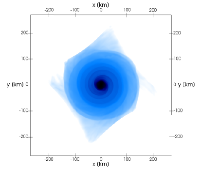
Figure 9: An equatorial slice of density in the hypermassive neutron star and disk configuration (Sec. IV.1).

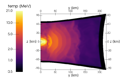
Figure 10: A meridional slice of temperature in the hypermassive neutron star and disk configuration (Sec. IV.1).

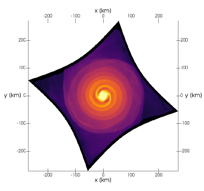
Figure 11: An equatorial slice of temperature in the hypermassive neutron star and disk configuration (Sec. IV.1).

We extrapolate the fluid and M1 radiation data from the domain shown in Figs. 8–11 to a larger ray tracing domain by setting all fluid and M1 radiation variables to their floor values outside the smaller domain. This simple extrapolation is adequate for ray tracing since the neutrinos are almost entirely free-streaming outside the smaller domain. Since the metric data were evolved on this larger domain no extrapolation is needed for them. The larger domain is represented as a pseudospectral grid composed of a sphere with concentric shells extending to $r\approx 1400$ km. Radial grid spacings are $\Delta r\approx 0.15$ km in the star and $\Delta r\approx 2.5$ km in the disk, with 12 cells spanning polar angles $\theta\in[0,\pi]$ and 24 cells spanning azimuthal angles $\phi\in[0,2\pi)$. Though a pseudospectral representation of non-smooth hydrodynamic data introduces some Gibbs-like oscillations in the variables, we choose to use this representation instead of the mesh-refined finite difference grid of the evolution because the pseudospectral representation uses much less memory: 95 MB in pseuspectral vs. 3 GB in finite difference representation. Obviously, memory loads of this order are not insurmountable; but they would require some modifications to our volume data interpolation infrastructure. For the purposes of this analysis the pseudospectral representation is adequate.

Opacities are computed from the LS220 equation of state using NuLib and are stored as a table covering energy, density, temperature, and composition ranges spanning $\varepsilon\in[1,280.5]$ MeV logarithmically, $\varrho\in[10^{6},3.2\times 10^{15}]\,{\rm g}\,{\rm cm}^{-3}$ logarithmically, $T\in[0.05,150]$ MeV logarithmically, and $Y_{e}\in[0.035,0.55]$ linearly, with grid extents $\{18,82,65,51\}$ respectively.

We place stationary (i.e. Eulerian) observers at fixed coordinate radius $r=250$ km in the $y$-$z$ plane along an arc at $N_{\theta}$ positions distributed linearly in $\cos\theta$ over the northern hemisphere using $\theta_{i}=\cos^{-1}\left(1-i/(N_{\theta}-1)\right)$ for $i=0,1,2,\ldots N_{\theta}-1$. We choose $N_{\theta}=30$.

Though the ray tracing sampling of $f$ is done in full general relativity, in our calculation of moments at the observer positions, we make the simplifying assumption of Minkowski spacetime. The errors in our moments introduced by this assumption may be estimated to be of order $GM/r=4\,{\rm km}/250\,{\rm km}$ (with $G$ the gravitational constant and $M$ the central mass), or $\sim 1\%$.

Each observer samples the distribution function over a uniform grid in energy, cosine of polar angle, and azimuthal angle with extents $\{N_{\tilde{\varepsilon}},N_{A},N_{B}\}$ spanning the ranges $\tilde{\varepsilon}\in(0,100)$ MeV, $\cos A\in\left((\cos A)_{\rm min},1\right)$, and $B\in[0,2\pi)$. The integrals for fluxes of number and energy (Eqns. 29, 32, and 33) become sums over all rays. Taking these fluxes in the radial direction, and using the midpoint rule to convert the integral to a sum, we have

$$\tilde{K}^{r}(\theta) =\frac{\Delta}{(2\pi)^{3}}\sum\limits_{m=0}^{N-1}\tilde{\varepsilon}_{m}^{2}\cos A_{m}f_{m}(\theta),$$ (60)

$$\tilde{H}^{r}(\theta) =\frac{\Delta}{(2\pi)^{3}}\sum\limits_{m=0}^{N-1}\tilde{\varepsilon}_{m}^{3}\cos A_{m}f_{m}(\theta),$$ (61)

with $f_{m}(\theta)\equiv f(\theta;\tilde{\varepsilon}_{m},\cos A_{m},B_{m})$, $\Delta\equiv\Delta\tilde{\varepsilon}\,\Delta(\cos A)\,\Delta B$, $N\equiv N_{\tilde{\varepsilon}}\,N_{A}\,N_{B}$, and $m$ the index labeling each ray. Average energies in the coordinate frame are given by $\langle\tilde{\varepsilon}\rangle(\theta)=\tilde{H}^{r}(\theta)/\tilde{K}^{r}(\theta)$. We choose $N_{\tilde{\varepsilon}}=30$, $N_{A}=150$, and $N_{B}=20$. To maintain high angular resolution, we only sample rays that pass within approximately 120 km of the star’s center by setting $(\cos A)_{\rm min}=0.88$.

We also combine measurements from all observers to estimate total luminosities and averages over the sky. Since we have chosen an arc of observers isolated to the northern hemisphere and the $y$-$z$ plane, we may extend these data to the full sky by assuming that emission is azimuthally symmetric and reflection symmetric across the equatorial plane. Figs. 8–11 indicate the approximate validity of these assumptions at 11 ms after merger. Total luminosities are then computed as integrals of the radial fluxes over $\cos\theta$. Using the trapezoid rule, the number and energy luminosities become sums:

$$R =C\left(\frac{1}{2}(\tilde{K}^{r}_{0}+\tilde{K}^{r}_{N_{\theta}-1})+\sum\limits_{n=1}^{N_{\theta}-2}\tilde{K}^{r}_{n}\right),$$ (62)

$$L =C\left(\frac{1}{2}(\tilde{H}^{r}_{0}+\tilde{H}^{r}_{N_{\theta}-1})+\sum\limits_{n=1}^{N_{\theta}-2}\tilde{H}^{r}_{n}\right),$$ (63)

with $C\equiv 2\pi r^{2}\,\Delta(\cos\theta)$, $\tilde{K}^{r}_{n}\equiv\tilde{K}^{r}(\theta_{n})$, $\tilde{H}^{r}_{n}\equiv\tilde{H}^{r}(\theta_{n})$, and $n$ labeling each observer’s position. Average energies over the whole sky are then $\langle\tilde{\varepsilon}\rangle=L/R$. Note, for simplicity we use the coordinate radius $r$ in this expression even though the earlier merger evolution did not necessarily produce areal coordinates. The effect of this choice is to artificially scale the ray tracing luminosities by some factor we believe to be very close to 1. In future work we can correct this error by computing the proper area over coordinate spheres at the observers’ locations.

Tab. 3 compares the all-sky luminosities and average energies from ray tracing and from the M1 transport simulation, which serves for qualitative comparison. Even if M1 and ray tracing methods both provide faithful measurements of all-sky luminosities, we expect some disagreement since the two treatments differ fundamentally. In addition to differences in transport methodologies, the M1 fluxes are integrated over the outer boundary of the finite-difference grid at radii ranging from 75 km to 200 km, whereas the ray tracing fluxes are integrated over a sphere at radius 250 km, introducing a time lag between some of the fluxes used in the measurements of order one millisecond. Additionally, uncertainties for the M1 simulation may be estimated from comparisons between M1 methods to be around 15% for energy luminosities and 10% for average energies (Foucart et al., 2016b, Sec. A.6).

Table 3: Comparison of total luminosities and average energies of the hypermassive neutron star configuration (presented in Sec. IV.1). The methods are ray tracing using the noscat method ‘noscat’, ray tracing using the gray scat method ‘scat’, and the M1 transport simulation ‘M1’. The ray tracing totals were computed from sums over observers placed in the $y$-$z$ plane. M1 values are taken from (Foucart et al., 2016b, Figs. 7, 9, 10). Energy luminosities have units $10^{52}\,{\rm erg}\,{\rm s}^{-1}$, number luminosities $10^{57}\,{\rm s}^{-1}$, and average energies MeV. The $\nu_{x}$ luminosities are per-species: multiply by four to get the total heavy-lepton neutrino luminosities.

	noscat	scat	M1
$L_{\nu_{e}}$	5.87	5.40	5
$L_{\bar{\nu}_{e}}$	9.70	10.7	12
$L_{\nu_{x}}$	23.6	12.5	12
$R_{\nu_{e}}-R_{\bar{\nu}_{e}}$	-0.91	-1.68	-2
$\langle\varepsilon_{\nu_{e}}\rangle$	12.7	12.0	12
$\langle\varepsilon_{\bar{\nu}_{e}}\rangle$	16.0	14.8	15
$\langle\varepsilon_{\nu_{x}}\rangle$	34.2	23.3	26

Because the model was evolved with a gray M1 transport scheme, the only scat method we can use in our ray tracing is the gray method. As in the post-bounce configuration in Sec. III.5, the scat treatment is more faithful than the noscat treatment, significantly so for the heavy-lepton neutrinos. For example, with scattering turned off the ray tracing and M1 measurements of $L_{\nu_{x}}$ disagree by 200%; but with scattering turned on agreement is within 10%. As the ray tracing and M1 measurements both show, $R_{\bar{\nu}_{e}}$ dominates over $R_{\nu_{e}}$ significantly, because the disrupted neutron star material is releptonizing.

The distributions of radial fluxes over observer position are shown in Figs. 12 and 13. With the noscat treatment the $\nu_{x}$ luminosities are relatively constant in $\theta$, because the disk is optically thin to $\nu_{x}$, and most of the heavy-lepton neutrinos come from the hypermassive neutron star, which is roughly spherical. The slight upward trend in $\nu_{x}$ luminosities with $\theta$ may be due to asymmetries in the fluid configuration, inhomogeneous coordinate maps used in the hydrodynamics evolution, or the fact that equatorial observers are closer to the disk’s hot spiral arms than are polar observers. It is not due to the Doppler shift or relativistic beaming from the rapid rotation of the star, a hypothesis we tested by setting $u_{i}=0$ and $W=1$ in the ray tracing equations. Because of their larger absorption cross section, the disk is not optically thin to $\nu_{e}$ and $\bar{\nu}_{e}$, and observers at small angles within view of the hot hypermassive neutron star measure the largest radial fluxes of these species. When we turn on scattering, the disk is no longer transparent to $\nu_{x}$, and $\nu_{x}$ luminosities present the same qualitative $\theta$-dependence as that of the other species.

Figure 12: Radial number fluxes, $\tilde{K}^{r}(\theta)$, as defined in Eqn. 60, in the hypermassive neutron star configuration (presented in Sec. IV.1). Sampled for observers at fixed coordinate distances from the center of the star, with $r=250\,{\rm km}$.

Figure 13: Same as Fig. 12 but radial energy fluxes $\tilde{H}^{r}(\theta)$ as defined in Eqn. 61.

From Figs. 12 and 13 we also see that for observers near the poles ($\theta\sim 0^{\circ}$) scattering generally increases fluxes of $\bar{\nu}_{e}$ and $\nu_{x}$ and decreases fluxes of $\nu_{e}$. When scattering is turned on, all three fluxes experience a similar loss of neutrinos from the central star. But the $\bar{\nu}_{e}$ and $\nu_{x}$ fluxes experience a more dominant gain of high energy neutrinos scattered by the disk back to the observer. The $\nu_{e}$ fluxes, however, experience only a minor gain of neutrinos from the disk, since $\nu_{e}$ presents a lower average energy, and the scattering cross-section depends strongly on energy. For observers in the equatorial plane ($\theta\sim 90^{\circ}$) the effect of scattering is a decrease in energy fluxes for all species. This is because more matter pollutes the equatorial regions than the polar regions, causing the losses from the star to dominate over the gains from the disk for all three species.

Fig. 14 shows the distribution of average energies of radial fluxes over observer positions. With and without scattering, the average energies are highest for observers near the polar axis, since polar observers get a direct view of the hot hypermassive neutron star. (This trend is unexpectedly reversed for $\nu_{x}$, and may be due to asymetries in the disk, as discussed above.) Scattering decreases average energies across all observer positions, as it did in the post-bounce configuration, or any configuration of a hot interior surrounded by a scattering envelope. The strength of the effect of scattering on the average energies of the different species is seen to follow the ranking $\nu_{x}>\bar{\nu}_{e}>\nu_{e}$ due to two factors: the average energies of the spectra obey the same ranking, and the thicknesses of the different species’ scattering envelopes also obey the same ranking. As we showed in the models with a homogeneous background scattering field, the scattering contribution $f_{\rm SE}$ is proportional to energy $\varepsilon^{2}$ and path length $s$ (Eqn. 55).

Figure 14: Same as Fig. 12 but average energies of radial fluxes $\langle\tilde{\varepsilon}\rangle(\theta)=\tilde{H}^{r}(\theta)/\tilde{K}^{r}(\theta)$, as defined in Eqns. 60 and 61.

In Figs. 15 and 16, we show the distributions of neutrino number density over incoming polar angle $\cos A$ for the observer on the polar axis $\theta=0^{\circ}$, and in the equatorial plane $\theta=90^{\circ}$. This number density is defined

$$\tilde{G}(\cos A) =\frac{\Delta}{(2\pi)^{3}}\sum\limits_{m=0}^{N-1}\tilde{\varepsilon}_{m}^{2}f_{m}(\cos A),$$ (64)

with $\Delta\equiv\Delta\tilde{\varepsilon}\Delta B$, $N\equiv N_{\tilde{\varepsilon}}N_{B}$, $f_{m}(\cos A)\equiv f(\tilde{\varepsilon}_{m},\cos A,B_{m})$, and $m$ the index labeling each ray at polar angle $\cos A$. The integral of this quantity over $d\cos A$ gives the total number density $\tilde{G}$, according to Eqn. 31. As in the case of the collapse profile in Sec. III.5, the dominant effect of elastic scattering on $\tilde{G}(\cos A)$ is to spread the distribution out to larger angles, by generally decreasing the number of neutrinos coming from the core while increasing the number of neutrinos coming from the disk.

For the observer in the equatorial plane, Fig. 16, the disk is so optically thick to $\nu_{e}$ that there is very little difference between scat and noscat treatments for incoming angles $\cos A\gtrsim 0.95$ corresponding to the volume inside of $r\lesssim 80$ km. Also the stepped temperature gradient in the disk’s spiral arms visible in Figs. 10 and 11 presents as a stepped heavy-lepton neutrino number density distribution in Fig. 16 in the noscat treatment, since the energy emission due to $e^{-}e^{+}$ annihilation, producing $\nu_{x}$, is especially sensitive to temperature, going as $T^{9}$ (Burrows et al., 2006, Sec. 7). This stepped distribution is not visible in $\nu_{e}$ and $\bar{\nu}_{e}$ emission, since we ignore pair processes for these species due to the dominance of absorption and emission processes, obeying a shallower temperature-dependence; nor is it visible in the scat treatment of $\nu_{x}$, since scattering tends to smear the incoming angle of the emission; nor is it visible for any species or treatment in Fig. 15, since the integration over the azimuthal angle $B$ averages out any spiral structure for the observer on the polar axis.

Figure 15: Distribution of number density $\tilde{G}(\cos A)$ over incoming angle, defined in Eqn. 64. The integral of this quantity over $d\cos A$ gives the total number density measured by this observer on the rotation axis. Volume data from the hypermassive neutron star configuration (presented in Sec. IV.1).

Figure 16: Distribution of number density $\tilde{G}(\cos A)$ over incoming angle, as in Fig. 15, but with the observer in the equatorial plane.

IV.2 Neutrino Oscillations at High Neutrino Densities

Here we examine the importance of elastic scattering in neutrino flavor oscillation above the hypermassive neutron star–disk configuration presented in Sec. IV.1. Our treatment of the flavor evolution equation assumes flat space and small fluid velocities. In consequence we treat some of the gauge-dependent quantities inconsistently, and we ignore potentially important features of relativistic flavor evolution near compact objects Yang and Kneller (2017). We believe our treatment is sufficient, however, for the following qualitative exploration.

The Boltzmann Equation (Eqn. 8) is one limiting form of the quantum kinetic equations for neutrinos Vlasenko et al. (2014), the limit where collisional mean free paths are much shorter than oscillation lengths, i.e. $\varepsilon/\mathscr{K}\ll|H|^{-1}$ with $H$ the Hamiltonian matrix describing coherent forward scattering interactions. In this limit the neutrino density matrix takes the form

$$\rho_{0}(\varepsilon,\ell_{\mu})=\sum\limits_{\alpha}f^{\nu_{\alpha}}(\varepsilon,\ell_{\mu})\ket{\nu_{\alpha}}\bra{\nu_{\alpha}},$$ (65)

with $\ket{\nu_{\alpha}}$ the neutrino flavor eigenstates. The neutrino state remains pure, or diagonal in the flavor basis.

But at the opposite limit, in the free-streaming regime, coherence effects become important, and the quantum kinetic equations take a Schrödinger-like form:

$$i\frac{d}{ds}S=HS,$$ (66)

where $ds$ is an interval of proper length traversed by the neutrino as measured by our observer, and $S$ is the neutrino flavor evolution matrix describing a mixed state

$$\rho=S\,\rho_{0}\,S^{\dagger}.$$ (67)

In this limit, we may decompose the Hamiltonian matrix into vacuum, matter, and neutrino contributions:

$$H=H_{\rm V}+H_{e}+H_{\nu\nu}.$$ (68)

Explicit formulas for these matrices may be found in the oscillation literature, e.g. Duan and Kneller (2009), but for clarity we only give their order-of-magnitude scales here:

$$|H_{\rm V}| \sim\frac{\Delta m^{2}}{\varepsilon},$$ (69)

$$|H_{e}| \sim G_{\rm F}\left|n_{e^{-}}-n_{e^{+}}\right|,$$ (70)

$$|H_{\nu\nu}| \sim G_{\rm F}\left|G_{\nu_{e}}-G_{\bar{\nu}_{e}}\right|,$$ (71)

where $\Delta m^{2}$ is the mass-squared differences between neutrino mass eigenstates, $G_{\rm F}$ is the Fermi coupling constant, $n_{e^{-}}$ and $n_{e^{+}}$ are the electron and positron number densities, and $G_{\nu_{e}}$ and $G_{\bar{\nu}_{e}}$ the electron neutrino and antineutrino number densities defined in Eqn. 31. In this statement of scale for $H_{\nu\nu}$ we only include the isotropic components of the neutrino fields; for our calculations below, however, we include the full angular distributions found via ray tracing.

In regimes in which $|H_{\nu\nu}|\ll|H_{\rm V},H_{e}|$, the flavor evolution is locally soluble in a ray-by-ray method, and reveals a rich and physically important phenonenology including vacuum, solar, atmospheric, and terrestrial oscillations, as well as oscillations in supernova envelopes. Where neutrino densities are relatively high, however, as in neutron star mergers, the problem must be solved globally. To date, no method has been devised to handle this problem in systems lacking spherical symmetry.

However, we can solve a similar but tractable problem along a single ray. We assume that all the neutrino rays intersecting an event along a given test ray have undergone the same flavor evolution history as that of the test ray: i.e. the evolution matrix $S$ is the same for all rays sharing that event. This is the so-called single-angle approximation, which is widely used in the supernova oscillation literature and has been shown to be qualitatively faithful in those environments. We note, however, that recent studies have discovered 1) spherically symmetric configurations for which a single-angle calculation produces qualitatively different flavor evolution behavior than a full multi-angle calculation Vlasenko and McLaughlin (2018), and 2) azimuthally-symmetric configurations for which the single-angle approximation masks certain instabilities in the flavor evolution Wu and Tamborra (2017).

The formalism of the single-angle approximation requires knowledge of the unoscillated neutrino contribution to the Hamiltonian matrix along a given test trajectory. This is a function of the unoscillated neutrino self-interaction potential, which for the $\alpha$-th flavor is:

$$V_{\nu_{\alpha},0}(\varepsilon,\ell_{\mu})=\frac{\sqrt{2}G_{\rm F}}{(2\pi)^{3}}\varepsilon^{2}\oint d\Omega^{\prime}(1-\omega^{\prime})f^{\nu_{\alpha}}(\varepsilon,\ell^{\prime}_{\gamma}),$$ (72)

with the test ray propagating in direction $\ell_{\mu}$, ambient rays propagating in directions $\ell^{\prime}_{\gamma}$, and the cosine of the angle between these given by $\omega^{\prime}=\psi^{\mu\gamma}\ell_{\mu}\ell^{\prime}_{\gamma}$. As in the moment equations (Eqns. 28-32), the integral is taken over all directions $\ell^{\prime}_{\gamma}$.

Implementing the single-angle approximation, we first use ray tracing to compute the unoscillated neutrino self-interaction potentials $V_{\nu_{\alpha},0}$ at several points along a test neutrino trajectory. We then integrate the flavor evolution matrix $S$ along this test trajectory, interpolating $V_{\nu_{\alpha},0}$ to all points sampled by the integration. And at each integration step we rescale $V_{\nu_{\alpha},0}$ according to the mixing specified by $S$.

If conditions are right, a resonant flavor transition introducing significant mixing may occur very near the point where neutrinos begin free-streaming. The matter-neutrino resonance Malkus et al. (2012, 2014, 2016), can occur where the matter potential and neutrino self-interaction potentials cancel, or where $V_{e}+V_{\nu\nu,0}=0$, with

$$V_{e} =\sqrt{2}G_{\rm F}\frac{\varrho}{m_{N}}Y_{e},$$ (73)

$$V_{\nu\nu,0} =\int d\varepsilon\big{(}V_{\nu_{e},0}(\varepsilon)-V_{\bar{\nu}_{e},0}(\varepsilon)\big{)},$$ (74)

with $\varrho$ the rest density and $m_{N}$ the nucleon mass. The matter potential $V_{e}$ is always positive; and far outside the accretion disks formed in neutron star mergers, in which the disrupted neutron-star matter is rapidly releptonizing, the total unoscillated neutrino self-interaction potential $V_{\nu\nu,0}$ is large and negative.

We examine this effect in the post-merger configuration already analyzed in Sec. IV.1. We calculate the self-interaction potential along a radial coordinate trajectory making an angle $\theta=25^{\circ}$ with the rotation axis, at $N_{r}=7$ positions $r\in\{30,50,82,135,223,368,608\}$ km. We sample distribution functions at each of these positions over a grid with extents $N_{\varepsilon}=30$, $N_{A}=200$, $N_{B}=30$; energies range over $\varepsilon\in(0,100)$ MeV; polar angles range over $\cos A\in((\cos A)_{\rm min},1)$, with $(\cos A)_{\rm min}\in\{-1,-1,-1,0.488,0.849,0.947,0.981\}$ for each of the $N_{r}$ positions; and azimuthal angles range over the whole sky $B\in[0,2\pi)$. We interpolate the logarithm of the self-interaction potentials (Eqn. 72) in path length $\log r$ along the ray, by fitting a 3rd order spline with continuous derivative, across the $N_{r}$ observation points. For $r>608$ km we extrapolate the self-interaction potentials using the geometric fall-off of $r^{-4}$ applicable to the far-field limit of the self-interaction potential Malkus et al. (2016).

The matter potential along this test ray is from an analytic wind model qualitatively consistent with the densities in the simulated volume (i.e. inside $r\sim 70$ km) and asymptoting to the $r^{-2}$ density field of a spherical steady-state wind with a constant asymptotic velocity. The density and velocity fields of a spherical steady-state wind obey the continuity equation $\rho(r)v(r)r^{2}=\rho_{1}v_{1}r_{1}^{2}$, with $\rho_{1}$ and $v_{1}$ the density and velocity measured at some fiducial radius $r_{1}$. For velocity field we choose a phenomenological wind model used in the oscillation literature Surman and McLaughlin (2005)

$$v(r)=v_{1}\left(1-\frac{R}{r_{1}}\right)^{-\beta}\left(1-\frac{R}{r}\right)^{\beta},$$ (75)

with $R$ the wind launch radius and $\beta$ an acceleration parameter. This yields the following density field

$$\rho(r)=\rho_{1}C\left[\frac{r_{1}}{R}\right]\left(1-\frac{R}{r}\right)^{-\beta}\left(\frac{R}{r}\right)^{2},$$ (76)

with $C[a]=a^{2-\beta}(a-1)^{\beta}$. We use the parameters $R=10$ km, $r_{1}=50$ km, $\beta=2$, and $\rho_{1}=10^{7}\,{\rm g}\,{\rm cm}^{-3}$. Additionally we impose a density cap of $\rho_{\rm max}=10^{14}\,{\rm g}\,{\rm cm}^{-3}$ inside the radius $r_{0}=5$ km, and smoothly interpolate densities between $r_{0}$ and $r_{1}$ with a cubic polynomial, enforcing $C^{0}$ and $C^{1}$ continuity at the transitions. The rest density from this model is plotted in Fig. 17. To translate this density field to a matter potential, we assume a constant electron fraction of $Y_{e}=0.5$, roughly consistent with the composition of the matter in the disk’s funnel (Foucart et al., 2016b, Fig. 8).

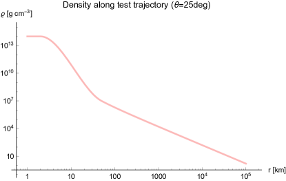
Figure 17: Assumed matter density along the neutrino test trajectory used to calculate the matter potential $V_{e}$.

In fact, a spherical steady-state wind model, though providing an adequate backdrop for the qualitative study presented in this section, is less than ideal for this post-merger configuration, most obviously because in the 10 ms since merger, ejecta with the greatest velocities around $0.3c$ will have reached no further than $r_{\rm max}\sim 10^{8}$ cm. Additionally, the true radial profile of the ejecta from this merger (which our computational model does not follow) will have many more features inside this radius, including shock jumps. However, this model density profile is adequate as a backdrop to our study here since we expect the remnant to present similar neutrino emission over a thermal timescale of a few tens of milliseconds while the matter field propagates out to larger radii.

In Figs. 18 and 19 we show the total unoscillated self-interaction potential and its contributions from $\nu_{e}$ and $\bar{\nu}_{e}$ for a test neutrino moving out along the radial coordinate trajectory described above. Fig. 18 shows these terms for the noscat treatment, and Fig. 19 for the scat treatment. Obviously, including the effects of elastic scattering tends to increase the $\bar{\nu}_{e}$ contribution relative to the $\nu_{e}$ contribution, in this case causing the self-interaction potential to be negative along the entire trajectory. This effect may be predicted from Fig. 15, which is calculated for a qualitatively similar observer, in the vacated polar funnel of the disk: in the scat treatment $G_{\bar{\nu}_{e}}$ dominates over $G_{\nu_{e}}$ at all angles $\cos A\lesssim 0.998$; whereas in the noscat treatment $G_{\bar{\nu}_{e}}$ only dominates over $G_{\nu_{e}}$ over a range of forward-peaked angles $\cos A\in(0.965,0.998)$. An additional factor supporting this trend is that neutrinos from the most forward-peaked angles $\cos A\sim 1$ have a suppressed effect on the self-interaction potential due to the $(1-\cos A)$ term arising in the integral of Eqn. 72.

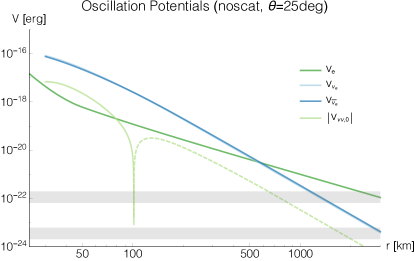
Figure 18: Neutrino oscillation potentials for the noscat case along a test trajectory originating at the surface of the hypermassive neutron star, and proceeding outward along a radial coordinate ray with angle $\theta=25^{\circ}$ with respect to the polar axis. The trajectory is parameterized by the coordinate radius $r$. We plot the vacuum potential due to mass-squared differences (gray bands), the matter potential $V_{e}$ due to forward scattering on $e^{-}$ and $e^{+}$ (dark green), and the self-interaction potential $V_{\nu\nu,0}$ due to forward scattering on ambient neutrinos (light green, solid where positive, dashed where negative); additionally we plot the $\nu_{e}$ and $\bar{\nu}_{e}$ components composing the self-interaction potential (light blue and dark blue respectively). The two gray bands at $V\sim 10^{-22}$ erg and $V\sim 10^{-24}$ erg indicating the two vacuum energy scales for 10–30 MeV neutrinos, set the positions of possible Mikheyev-Smirnov-Wolfenstein (MSW) or nutation resonances Malkus et al. (2012). Inside the symmetric point at $r\sim 100\,{\rm km}$ the total unoscillated self-interaction potential $V_{\nu\nu,0}$ is positive, i.e. $\nu_{e}$-dominated.

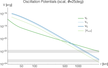
Figure 19: Same as Fig. 18, but for the scat case. Unlike the case with scattering turned off, here the total unoscillated self-interaction potential $V_{\nu\nu,0}$ is everywhere negative, i.e. $\bar{\nu}_{e}$-dominated.

We also solve for the flavor evolution of this system, integrating $S$ according to Eqn. 66, as described in Zhu et al. (2016). We show the survival probabilities for $\nu_{e}$ and $\bar{\nu}_{e}$ in Figs. 20 and 21, comparing the noscat and scat treatments. In these figures we also show the evolved self-interaction potential $V_{\rm osc}$,

$$V_{\rm osc}\equiv(H_{\nu\nu})_{ee}-{\rm Tr}(H_{\nu\nu})/3,$$ (77)

to show how the neutrino interactions driving the oscillation evolve with flavor. Note that $V_{\rm osc}$ is identical to $V_{\nu\nu,0}$ if no flavor evolution takes place. The survival probability is the probability that a neutrino, if measured, will be found to be in its original flavor state. The survival probabilities are computed at each point along the trajectory from the absolute square of the diagonal terms of the flavor evolution matrix, $P_{\nu_{\alpha}\to\nu_{\alpha}}=|S_{\alpha\alpha}|^{2}$. When $P_{\nu_{e}\to\nu_{e}}$ decreases, as can be seen for example in Fig. 21 for $r>400$ km, some of the $e$ neutrinos have oscillated into $\mu$ or $\tau$ neutrinos.

Fig. 20 shows the survival probabilities from the calculation with elastic scattering turned off. Using neutrino mixing angle $\theta_{12}$ and the inverted hierarchy (the normal hierarchy gives qualitatively similar results) electron neutrinos and antineutrinos start to oscillate around 700 km in the form of a collective neutrino oscillation, causing both $\nu_{e}$ and $\bar{\nu}_{e}$ to convert to heavy lepton neutrinos and antineutrinos respectively. A similar effect was seen in Frensel et al. (2017); Tian et al. (2017). Fig. 21 shows the survival probabilities of an otherwise identical calculation, but with elastic scattering turned on. In this case, electron neutrinos and antineutrinos start to oscillate around 400 km in the form of a standard matter neutrino resonance: at first both $\nu_{e}$ and $\bar{\nu}_{e}$ convert to heavy lepton neutrinos, but as the transformation progresses, the $\bar{\nu}_{e}$ partially return to their original flavor.

Note that during the latter part of the matter neutrino resonance depicted in Fig. 21, where the self-interaction potential approaches the vacuum scale, the survival probabilities show some small-scale oscillations different than the standard matter neutrino resonance introduced in Malkus et al. (2014). This occurs because the self-interaction potential and matter potential fall close to the vacuum potential scale.

The collective neutrino oscillation occuring in the noscat case (Fig. 20) not only produces a very different flavor mixture, the transformation also starts further from the remnant, and it extends much further before it completes. For these potentials along this test trajectory, we see that a matter-neutrino resonance only occurs in the scat case; though with a slightly higher matter potential it could occur in both cases, closer to the disk in the noscat case than the scat case. For this particular test trajectory we only see a standard and not a symmetric matter neutrino resonance Malkus et al. (2016); Väänänen and McLaughlin (2016). As we can see from these calculations, the final outcome of the flavor transformation is quite different in the two scenarios.

Figure 20: Neutrino survival probabilities for the noscat case. In the lower panel we show the matter potential $V_{e}$ from Fig. 18, and the evolved self-interaction potential $V_{\rm osc}$ from Eqn. 77. In this case, the neutrinos undergo collective neutrino oscillation beginning around $r\sim 700$ km, with both the electron neutrinos and antineutrinos converting to heavy-lepton neutrinos and antineutrinos almost completely.

Figure 21: Same as Fig. 20, but for the scat case. In this case the neutrinos undergo a standard MNR transition beginning around $r\sim 400$ km, with the electron neutrinos converting to heavy-lepton neutrinos almost completely, and the electron antineutrinos oscillating back to their original flavor after partially converting to heavy-lepton antineutrinos.

V Conclusions

We have introduced a new general relativistic ray tracing method to compute neutrino distribution functions around compact objects in dynamical configurations, and which incorporates the effects of elastic scattering for the first time within a ray tracing framework. Elastic scattering of neutrinos into and out of each ray is included in our method by using estimates of the background neutrino fields from an M1 transport simulation. To capture the energy spectrum of the background field, we have described a spectral method which uses neutrino energy densities over multiple energy groups as input, and a gray method which uses neutrino energy and number densities averaged over all energies as input. We have also successfully tested the ray tracing code with a comprehensive battery of tests.

In our tests (Sec. III) we have confirmed that elastic scattering plays a significant role in redistributing neutrino energy- and angle-distributions in common compact-object configurations. The largest effects are seen in $\nu_{x}$ distributions and to a lesser extent $\bar{\nu}_{e}$, with the dominant effect being a decrease in average energies from the central body, and an increase in average energies from the scattering envelope. More specifically, in the disk configuration formed by the merger of two neutron stars (Sec. IV.1), elastic scattering causes

1. a decrease in average energies of neutrinos emerging from the remnant at all angles and for all species,

2. an increase in $\bar{\nu}_{e}$ and $\nu_{x}$ fluxes and a decrease in $\nu_{e}$ fluxes viewed from along the rotation axis, and

3. a decrease in all species’ fluxes viewed from the equatorial plane.

Furthermore we find good agreement in overall number and energy luminosities and average energies in comparisons with neutrino transport methods, e.g. Monte Carlo in Sec. III.5 and M1 transport in Sec. IV.1.

We have also employed the ray tracing code to examine neutrino flavor oscillations along one sample trajectory exiting the neutrino-dense environment of the neutron star post-merger configuration (Sec. IV.2). The trajectory starts from 300 km, and moves out radially at $25^{\circ}$ from the polar axis. Along that trajectory, elastic scattering has the effect of increasing the ratio of $\bar{\nu}_{e}$ relative to $\nu_{e}$. This creates a negative self-interaction potential which introduces a complete standard matter neutrino resonance transition (see Fig. 21). At about 400 km from the merger core, both electron neutrinos and electron antineutrinos begin to transform. At about 1200 km $e$ neutrinos have almost completely converted to $\mu$ or $\tau$ neutrinos, while the $e$ antineutrinos have returned back to their original flavor. In an otherwise identical calculation, ignoring elastic scattering causes the flavor transformation to be very different (see Fig. 20).

This example demonstrates the importance of the physics of elastic scattering in the phenomenon of neutrino flavor oscillation. However, we avoid drawing general conclusions from this particular example, since a single astrophysical configuration can present dramatically different oscillation resonances along test trajectories emerging at different angles Zhu et al. (2016), and since the matter neutrino resonance is extremely sensitive to a host of parameters.

Finally, we propose the following improvements to the ray tracing code to make it a more useful and robust astrophysical simulation tool:

1. Use the finite-difference hydrodynamics simulation grid to represent background fluid and neutrino variables instead of interpolating all input variables to the pseudo-spectral spacetime simulation grid in order to begin ray tracing. We have found that though the interpolation of fluid and neutrino variables to a lower-resolution pseudo-spectral grid saves computational memory, it introduces more costly problems, the foremost being Gibbs-like oscillations at shocks and discontinuities present in fluid fields.

2. Replace explicit with implicit time stepping in the integrations along each ray. We have found that the stability of the time-integration demands extremely small step sizes of the adaptive time-stepping algorithm, especially for higher-energy rays. Large errors are possible if time-stepping thresholds are not fine-tuned to each new configuration.

3. Improve the spectral assumptions made in the gray method. The test of both gray and spectral methods against the fiducial Monte Carlo calculation presented in Sec. III.5 indicated strong agreement for overall average energies for all species. However, the average energy of $\bar{\nu}_{e}$ emerging from the envelope (which contributed only a tiny fraction to the total luminosity) differed between the gray treatment and the Monte Carlo by 30%. Agreement could be improved with better spectral assumptions, for example employing pinched spectra.

Acknowledgements

This work was supported in part by the National Science Foundation under Grant No. PHY-1430152 (JINA Center for the Evolution of the Elements) [MBD, YLZ, GCM]; by NASA through the Hubble Fellowship under grant 51344.001-A, awarded by the Space Telescope Science Institute, which is operated by the Association of Universities for Research in Astronomy Inc. for NASA under contract NAS 5-26555 [EO]; by NASA through the Einstein Postdoctoral Fellowship grant PF4-150122 awarded by the Chandra X-ray Center, which is operated by the Smithsonian Astrophysical Observatory for NASA under contract NAS8-03060, and through grant 80NSSC18K0565 [FF]; through National Science Foundation Grant PHY-1402916 [MDD]; and through the U.S. Department of Energy, Office of Science, Office of Nuclear Physics, under award number DE-FG02-02ER41216 [GCM]. We thank James P. Kneller for his original flavor evolution code base. We thank the Spectral Einstein Code collaboration for a powerful and robust numerical relativity code base, and in particular Lawrence E. Kidder, Daniel A. Hemberger, François Hébert, and Fatemeh Hossein Nouri for comments and help throughout. We also thank Sherwood Richers for providing his neutrino transport code Sedonu for comparisons, and Luke Roberts for helpful discussions at the JINA-CEE Frontiers meeting 2017.

Appendix A Definitions

We decompose the neutrino momentum into components parallel and orthogonal to an observer’s velocity $u_{\beta}$:

$$p_{\beta}=\varepsilon(u_{\beta}+\ell_{\beta}),$$ (78)

with $u_{\alpha}\ell^{\alpha}=0$ and $\ell_{\alpha}\ell^{\alpha}=1$.

We use two possible fiducial observers to define the momentum decomposition via Eqn. 78: the Eulerian, or normal observer $n_{\mu}=-\alpha\,\partial_{\mu}t$, and the fluid, or comoving observer $u^{\mu}=Wn^{\mu}+v_{\rm E}^{\mu}$. Here $t$ is coordinate time and $\alpha$ is the lapse in the standard 3+1 decomposition of the metric

$$\psi_{\mu\gamma}\rightarrow\left(\begin{matrix}-\alpha^{2}+\beta^{i}\beta_{i}&\beta_{i}\\ \beta_{j}&g_{ij}\end{matrix}\right).$$ (79)

We have also introduced the fluid Lorentz factor $W=\alpha u^{t}$, its Eulerian velocity $v_{\rm E}^{\mu}=g^{\mu}_{\lambda}u^{\lambda}$ (distinct from its coordinate velocity $v^{\mu}=u^{\mu}/u^{t}$), and the projection tensor orthogonal to the normal observer $g^{\mu}_{\lambda}=\psi^{\mu}_{\lambda}+n^{\mu}n_{\lambda}$.

We specify the neutrino direction in the observer’s frame with two spherical polar angles ($a$,$b$) with respect to the simulation cartesian coordinates

$$\ell_{\alpha} \rightarrow q(s,\Omega_{i}),$$ (80)

$$\Omega_{i} \rightarrow(\sin a\cos b,\sin a\sin b,\cos a),$$ (81)

or alternatively the two spherical polar angles ($A$,$B$) with respect to rotated coordinates

$$\Omega_{i^{\prime}}\rightarrow(\sin A\cos B,\sin A\sin B,\cos A).$$ (82)

The two coordinate systems are related by a standard Euler rotation of first $\phi$ about the $z$-axis, then $\theta$ about the rotated $y$-axis, with $\phi$ and $\theta$ the azimuthal and polar position of the observer. Expressed algebraically:

$$\Omega_{x} =\Omega_{x^{\prime}}\cos\theta\cos\phi-\Omega_{y^{\prime}}\sin\phi+\Omega_{z^{\prime}}\sin\theta\cos\phi,$$

$$\Omega_{y} =\Omega_{x^{\prime}}\cos\theta\sin\phi+\Omega_{y^{\prime}}\cos\phi+\Omega_{z^{\prime}}\sin\theta\sin\phi,$$

$$\Omega_{z} =\Omega_{x^{\prime}}\sin\theta+\Omega_{z^{\prime}}\cos\theta.$$ (83)

The scale factors $q$ and $s$ are functions of the neutrino direction $\Omega_{i}$, the observer’s velocity $u_{\alpha}$, and the spacetime metric. In the case of a fluid observer, specified by an arbitrary $W$ and $u_{i}$, $q$ and $s$ are given by

$$q =W\alpha\Bigg{(}2\beta^{i}\Omega_{i}W^{2}(\beta^{i}\Omega_{i}-1)$$

$$\qquad\qquad-2\Omega_{i}u_{j}g^{ij}W\alpha(\beta^{i}\Omega_{i}-1)$$

$$\qquad\qquad+\alpha^{2}\left((\Omega_{i}u_{j}g^{ij})^{2}+\Omega_{i}\Omega_{j}g^{ij}W^{2}\right)\Bigg{)}^{-1/2}$$ (84)

$$s =\beta^{i}\Omega_{i}-\Omega_{i}u_{j}g^{ij}.$$ (85)

In the case of an Eulerian observer, $W=1$ and $u_{i}=0$, and these expressions simplify considerably:

$$\tilde{q} =\alpha\left(2\beta^{i}\Omega_{i}(\beta^{i}\Omega_{i}-1)+\alpha^{2}\Omega_{i}\Omega_{j}g^{ij}\right)^{-1/2}$$ (86)

$$\tilde{s} =\beta^{i}\Omega_{i}.$$ (87)

In the even simpler case of Minkowski spacetime, these expressions reduce to $q=W/(1+s)$, $s=-\Omega_{i}u^{i}$, $\tilde{q}=1$, $\tilde{s}=0$.

In addition to the fluid velocity and Lorentz factor, described above, the other fluid state variables we use from our hydrodynamic simulations are rest density $\varrho=m_{b}n_{b}$, temperature $T$, and electron fraction

$$Y_{e}=\frac{n_{e^{-}}-n_{e^{+}}}{n_{b}},$$ (88)

where $n_{e^{-}}$, $n_{e^{+}}$, and $n_{b}$ are the number densities of electrons, positrons, and baryons, and $m_{b}$ is the average baryon mass.

Appendix B Source Terms

Here we present the sources comprising the right hand side of the Boltzmann Equation (Eqn. 8). The sources for the neutrino distribution function $f(x^{\alpha};p_{\beta})$ arise from collision processes producing, removing, or scattering to/from that point in phase space. The weak interaction rates for each process involve integrals of the neutrino distribution function $f(x^{\alpha};p^{\prime}_{\beta})$ and that of the antineutrino $\bar{f}(x^{\alpha};p^{\prime}_{\beta})$ over a momentum volume $dP^{\prime}$ (Eqn. 2).

We follow Bruenn (1985) and (Shibata et al., 2011, Sec. 4) by separating these processes into four categories:

$$C[f]\equiv C_{\rm AE}+C_{\rm SE}+C_{\rm SI}+C_{\rm PP},$$ (89)

representing charged-current absorption and emission, elastic scattering, inelastic scattering, and the thermal pair processes of annihilation and production. In this work, however, we only treat absorption/emission and elastic scattering. We seek to write each collision source linear in $f$:

$$C_{\rm AE} =\mathscr{E}_{\rm AE}-\mathscr{K}_{\rm AE}\,f,$$ (90)

$$C_{\rm SE} =\mathscr{E}_{\rm SE}-\mathscr{K}_{\rm SE}\,f.$$ (91)

Each term is computed by summing the weak interaction rates of the processes from the relevant category given in Tab. 1. We compute these rates in the rest frame of the fluid, but because they are spacetime invariants they take the same numerical value in any frame of reference and are completely independent of our choice of fiducial observer $u^{\alpha}$ (see discussion around Eqn. 9).

We compute our rates using the open source neutrino interaction library NuLib O’Connor (2015). We compile a table of sources defined over the four dimensions of density, temperature, electron-fraction, and neutrino energy, and interpolate quad-linearly to the points sampled along each ray.

Each source term is unique to the neutrino or antineutrino species modeled, and consists of a sum over all of the processes contributing to that category of interaction. For example: $C^{\nu_{e}}_{{\rm AE}}=\sum_{i}\,C^{\nu_{e}}_{{\rm AE},i}$, where $i$ labels the absorption/emission processes involving $\nu_{e}$ in Tab. 1. By contrast $C^{\nu_{x}}_{{\rm AE}}$ is formally equal to zero. However, in practice, NuLib implements the thermal pair processes via an effective emission/absorption term in order to avoid the need to couple energy groups and species (see Sec. B.4). This has been shown to work well for core-collapse supernovae O’Connor (2015).

B.1 Absorption and emission via charged current

At neutrino and thermal energies well below the masses of the muon or tauon ($m_{\mu}\sim 100\,{\rm MeV}$) only charged current processes involving $\nu_{e}$ and $\bar{\nu}_{e}$ are allowed. For each of these processes $i$ in Tab. 1, we may write an emission and absorption coefficient as a function of the interaction cross-section (e.g. (Bruenn, 1985, Eqn. A5)):

$$C_{{\rm AE},i} =\varepsilon j_{i}(1-f)-\varepsilon\chi_{a,i}f$$ (92)

$$=\varepsilon j_{i}-(\varepsilon j_{i}+\varepsilon\chi_{a,i})f,$$ (93)

where $j$ is the emissivity and $\chi_{a}$ the absorption opacity. Both $j$ and $\chi_{a}$ have dimension ${\rm length}^{-1}$ and represent the number of neutrinos emitted or absorbed per length traveled. In radiation transport formulations using specific intensities instead of distribution functions, an emissivity $\eta$ having dimension ${\rm energy}\,{\rm length}^{-3}\,{\rm time}^{-1}\,{\rm energy}^{-1}\,{\rm steradian}^{-1}$ is more commonly used. The two are related by $j=(2\pi)^{3}\eta/\varepsilon^{3}$. Note that for brevity we have suppressed the energy-dependence of the terms $j$, $\chi_{a}$, and the distribution functions.

In the special case of radiative equilibrium we know that the source term vanishes: an equal number of neutrinos are emitted from and absorbed by the matter for any length traversed. We also know in this case that the neutrino distribution function must be $f^{\rm eq}$, the equilibrium Fermi-Dirac distribution function of Eqn. 15. With these facts we can rearrange Eqn. 92 to give us Kirchoff’s Law:

$$j_{i} =\frac{\chi_{a,i}}{1-f^{\rm eq}}f^{\rm eq},$$ (94)

$$=\chi^{*}_{a,i}\,f^{\rm eq},$$ (95)

where in Eqn. 95 we have introduced the opacity corrected for stimulated absorption, $\chi^{*}_{a,i}$.

Using these expressions and computing the sum over stimulated opacities $\chi^{*}_{a,i}=\sum_{i}\chi^{*}_{a,i}$, the invariant emissivity and opacity for absorption/emission are

$$\mathscr{E}_{{\rm AE}} =\varepsilon\,\chi^{*}_{a}\,f^{\rm eq},$$ (96)

$$\mathscr{K}_{{\rm AE}} =\varepsilon\,\chi^{*}_{a}.$$ (97)

These expressions are equivalent to those in Eqns. 13 and 14.

We use the above treatment for $\nu_{e}$ and $\bar{\nu}_{e}$ only; the $\mu$ and $\tau$ neutrinos and antineutrinos do not participate in charged current absorption/emission interactions at these temperatures and energies. However we do use an effective stimulated absorption opacity $\chi^{*}_{a}$ for the heavy-lepton neutrinos, computed by NuLib as described in O’Connor (2015) which follows Bruenn (1985); Burrows et al. (2006). This is described in App. B.4.

B.2 Elastic scattering

Neutrino scattering on particles of mass much greater than $\varepsilon$ (i.e. nucleons and nuclei) is essentially iso-energetic. Following (Bruenn, 1985, Eqn. A8) or (Shibata et al., 2011, Eqn. 4.20) the collision term for the $i$-th process takes the form

$$C_{{\rm SE},i}(\ell_{\alpha})=\frac{\varepsilon^{3}}{(2\pi)^{3}}\oint d\Omega^{\prime}R_{{\rm SE},i}(\omega^{\prime})\Big{(}f(\ell^{\prime}_{\beta})-f(\ell_{\alpha})\Big{)}$$ (98)

where $R_{\rm SE,i}(\omega^{\prime})$ is the scattering kernel for the $i$-th process from direction $\ell^{\prime}_{\beta}$ to direction $\ell_{\alpha}$ having dimension ${\rm energy}^{-1}$, and the cosine of the scattering angle is $\omega^{\prime}\equiv\psi^{\alpha\beta}\ell_{\alpha}\ell^{\prime}_{\beta}$, with $\psi^{\alpha\beta}$ the inverse of the spacetime metric. Note that for brevity in Eqn. 98 we have suppressed the energy dependence of all of the terms.

It is customary to approximate the scattering kernel to linear order in $\omega$ (as in (Shibata et al., 2011, Eqn. 4.21)):

$$R_{{\rm SE},i}(\varepsilon,\omega)\approx R_{{\rm SE},i}^{0}(\varepsilon)+\omega\,R_{{\rm SE},i}^{1}(\varepsilon).$$ (99)

Using this definition and the moments defined in Eqns. 28 and 29, and writing $\omega^{\prime}=\ell_{\alpha}\ell^{\prime\alpha}$, we expand Eqn. 98 into four terms. The term containing $\oint d\Omega^{\prime}\ell^{\prime\alpha}$ vanishes by construction, and the remaining three terms may be written in the form

$$C_{{\rm SE},i}=\varepsilon\chi^{0}_{i}\Phi_{i}-\varepsilon\chi^{0}_{i}f,$$ (100)

where we have introduced the scattering opacity $\chi^{0}_{i}$ for each of the elastic scattering processes $i$ in Tab. 1 and the background scattering field $\Phi$:

$$\chi^{0}_{i}(\varepsilon) =\frac{4\pi\varepsilon^{2}}{(2\pi)^{3}}R_{{\rm SE},i}^{0}(\varepsilon),$$ (101)

$$\Phi_{i}(\varepsilon,\ell_{\alpha}) =\frac{(2\pi)^{3}}{\varepsilon^{3}}\frac{1}{4\pi}\left(J(\varepsilon)+\frac{\chi^{1}_{i}(\varepsilon)}{\chi^{0}_{i}(\varepsilon)}\ell_{\alpha}H^{\alpha}(\varepsilon)\right),$$ (102)

and with $\chi^{1}_{i}$ defined

$$\chi^{1}_{i}(\varepsilon)=\frac{4\pi\varepsilon^{2}}{(2\pi)^{3}}R_{{\rm SE},i}^{1}(\varepsilon).$$ (103)

Note that $\chi^{1}_{i}/\chi^{0}_{i}$ in Eqn. 102 is the degree of non-isotropy in the scattering. This term is roughly $-0.1$ for scattering on free neutrons, $-0.2$ on free protons, and $1$ on heavy nuclei; and at disk temperatures the composition is almost entirely free nucleons. Therefore in our treatment, for simplicity, we only retain the isotropic contribution to the background field:

$$\Phi(\varepsilon)=\frac{(2\pi)^{3}}{\varepsilon^{3}}\frac{1}{4\pi}J(\varepsilon).$$ (104)

Computing sums over the opacities $\chi_{s}\equiv\sum_{i}\chi^{0}_{i}$ and $\chi^{1}_{s}\equiv\sum_{i}\chi^{1}_{i}$, the invariant emissivity and opacity for elastic scattering are

$$\mathscr{E}_{\rm SE} =\varepsilon\,\chi_{s}\,\Phi,$$ (105)

$$\mathscr{K}_{\rm SE} =\varepsilon\,\chi_{s}.$$ (106)

We have made the energy-dependence of the background scattering field explicit in Eqn. 102. When we compute $\Phi(\varepsilon)$ using $J(\varepsilon)$ and $H^{\alpha}(\varepsilon)$ from a multi-group M1 transport evolution, we call this the spectral method.

However moment evolutions with multiple energy groups are still rare. Most simulations employ a gray moment scheme, evolving only the energy-integrated moments, $J$ and $H^{\alpha}$ and sometimes the number density $G$. If such is the case we resort to the gray method, by reconstructing the energy-dependent source terms from gray moments, assuming a diluted Fermi-Dirac spectrum. We use the following procedure:

1. Interpolate the fluid temperature, $T$, equilibrium neutrino chemical potential, $\eta_{\nu}$, and evolved neutrino energy and number densities in the fluid frame, $J$ and $G$, from the simulation grid.

2. Compute the average neutrino energy in the fluid frame

   $$\langle\varepsilon\rangle\equiv J/G.$$ (107)

3. Compute the neutrino spectral temperature, assuming equilibrium with the fluid

   $$T_{\nu}=\langle\varepsilon\rangle\frac{\mathscr{F}_{2}(\eta_{\nu})}{\mathscr{F}_{3}(\eta_{\nu})},$$ (108)

   where $\mathscr{F}_{b}$ is the Fermi integral

   $$\mathscr{F}_{b}(\eta)=\int_{0}^{\infty}dx\,x^{b}(1+e^{x-\eta})^{-1}.$$ (109)

   We implement the Fermi integrals using the analytical approximants from Takahashi et al. (1978).

4. Assume the background neutrino fields have the same total density as the evolved moments

   $$J(\varepsilon) =J\frac{\varepsilon^{3}}{T_{\nu}^{4}\,\mathscr{F}_{3}(\eta_{\nu})}\big{(}1+\exp(\varepsilon/T_{\nu}-\eta_{\nu})\big{)}^{-1},$$ (110)

   $$H^{\mu}(\varepsilon) =H^{\mu}\frac{\varepsilon^{3}}{T_{\nu}^{4}\,\mathscr{F}_{3}(\eta_{\nu})}\big{(}1+\exp(\varepsilon/T_{\nu}-\eta_{\nu})\big{)}^{-1}.$$ (111)

Note that to avoid floating point errors for very large negative $\eta$, we employ the asymptotic form of Eqn. 109: $\lim_{\eta\ll-1}\mathscr{F}_{b}(\eta)=b!\,e^{\eta}$. Thus, for $\eta<-10$, we use the limiting forms of Eqns. 108, 110, and 111:

$$T_{\nu} =\frac{\langle\varepsilon\rangle}{3},$$ (112)

$$J(\varepsilon) =J\frac{\varepsilon^{3}}{6T_{\nu}^{4}}e^{-\varepsilon/T_{\nu}},$$ (113)

$$H^{\mu}(\varepsilon) =H^{\mu}\frac{\varepsilon^{3}}{6T_{\nu}^{4}}e^{-\varepsilon/T_{\nu}}.$$ (114)

When we use the moments from Eqns. 110 and 111 in Eqn. 102, we call this the gray method.

B.3 Inelastic scattering

Neutrino scattering off of electrons is inelastic, changing the magnitude and direction of the neutrino’s momentum Bruenn (1985). In a supernova environment we expect inelastic scattering off of electrons and nucleons to shift the neutrino spectra to lower energies, most noticeably for heavy-lepton neutrinos Thompson et al. (2003). A similar formalism to the above could be used to derive source terms for inelastic scattering. We save that for future work, pointing out here that inelastic scattering treated this way is very sensitive to the energy-dependence of the background field. In this work we take $C_{\rm SI}=0$.

B.4 Thermal pair annihilation and production

We do not include thermal pair processes within the standard pair-process formalism; in other words we take $C_{\rm PP}=0$. But as mentioned in App. B.1, we do include these processes in an effective emission/absorption opacity for $\mu$ and $\tau$ neutrinos and antineutrinos. This has been shown to work well for core-collapse supernovae O’Connor (2015). Within NuLib, we compute the energy-dependent emissivity of the pair processes in Tab. 1, ignoring final state neutrino blocking. We then apply Kirchoff’s law, Eqn. 94, to convert this to an effective absorption opacity. We only use this effective opacity for heavy-lepton neutrinos because the charged-current emission/absorption processes for $\nu_{e}$ and $\bar{\nu}_{e}$ dominate in the environments we study: early merger remnants and supernovae.

References

- Ruffert et al. (1996) M. Ruffert, H.-T. Janka, and G. Schaefer, Astron. Astrophys. 311, 532 (1996), astro-ph/9509006 .
- Rosswog and Liebendörfer (2003) S. Rosswog and M. Liebendörfer, Mon.Not.Roy.Astron.Soc. 342, 673 (2003), arXiv:astro-ph/0302301 [astro-ph] .
- Deaton et al. (2013) M. B. Deaton, M. D. Duez, F. Foucart, E. O’Connor, C. D. Ott, L. E. Kidder, C. D. Muhlberger, M. A. Scheel, and B. Szilagyi, Astrophys. J. 776, 47 (2013), arXiv:1304.3384 [astro-ph.HE] .
- Galeazzi et al. (2013) F. Galeazzi, W. Kastaun, L. Rezzolla, and J. A. Font, Phys. Rev. D 88, 064009 (2013), arXiv:1306.4953 [gr-qc] .
- Perego et al. (2016) A. Perego, R. M. Cabezón, and R. Käppeli, Astrophys. J. Suppl. Ser. 223, 22 (2016), arXiv:1511.08519 [astro-ph.IM] .
- Radice et al. (2016) D. Radice, F. Galeazzi, J. Lippuner, L. F. Roberts, C. D. Ott, and L. Rezzolla, Mon. Not. Roy. Astr. Soc. 460, 3255 (2016), arXiv:1601.02426 [astro-ph.HE] .
- Abdikamalov et al. (2012) E. Abdikamalov, A. Burrows, C. D. Ott, F. Löffler, E. O’Connor, J. C. Dolence, and E. Schnetter, Astrophys. J. 755, 111 (2012), arXiv:1203.2915 [astro-ph.SR] .
- Richers et al. (2015) S. Richers, D. Kasen, E. O’Connor, R. Fernández, and C. D. Ott, Astrophys. J. 813, 38 (2015), arXiv:1507.03606 [astro-ph.HE] .
- Foucart et al. (2015) F. Foucart, E. O’Connor, L. Roberts, M. D. Duez, R. Haas, L. E. Kidder, C. D. Ott, H. P. Pfeiffer, M. A. Scheel, and B. Szilagyi, Phys. Rev. D 91, 124021 (2015), arXiv:1502.04146 [astro-ph.HE] .
- Foucart et al. (2016a) F. Foucart, R. Haas, M. D. Duez, E. O’Connor, C. D. Ott, L. Roberts, L. E. Kidder, J. Lippuner, H. P. Pfeiffer, and M. A. Scheel, Phys. Rev. D 93, 044019 (2016a), arXiv:1510.06398 [astro-ph.HE] .
- Thorne (1981) K. S. Thorne, Mon. Not. Roy. Astr. Soc. 194, 439 (1981).
- Shibata et al. (2011) M. Shibata, K. Kiuchi, Y. Sekiguchi, and Y. Suwa, Progress of Theoretical Physics 125, 1255 (2011), arXiv:1104.3937 [astro-ph.HE] .
- Kuroda et al. (2012) T. Kuroda, K. Kotake, and T. Takiwaki, Astrophys. J. 755, 11 (2012), arXiv:1202.2487 [astro-ph.HE] .
- Just et al. (2015) O. Just, M. Obergaulinger, and H.-T. Janka, Mon. Not. Roy. Astr. Soc. 453, 3386 (2015), arXiv:1501.02999 [astro-ph.HE] .
- O’Connor (2015) E. O’Connor, Astrophys. J. Suppl. Ser. 219, 24 (2015), arXiv:1411.7058 [astro-ph.HE] .
- Skinner et al. (2016) M. A. Skinner, A. Burrows, and J. C. Dolence, Astrophys. J. 831, 81 (2016), arXiv:1512.00113 [astro-ph.SR] .
- Roberts et al. (2016) L. F. Roberts, C. D. Ott, R. Haas, E. P. O’Connor, P. Diener, and E. Schnetter, Astrophys. J. 831, 98 (2016), arXiv:1604.07848 [astro-ph.HE] .
- Foucart et al. (2016b) F. Foucart, E. O’Connor, L. Roberts, L. E. Kidder, H. P. Pfeiffer, and M. A. Scheel, Phys. Rev. D 94, 123016 (2016b), arXiv:1607.07450 [astro-ph.HE] .
- Surman et al. (2011) R. Surman, G. C. McLaughlin, and N. Sabbatino, Astrophys. J. 743, 155 (2011), arXiv:1112.2673 [astro-ph.HE] .
- Roberts et al. (2017) L. F. Roberts, J. Lippuner, M. D. Duez, J. A. Faber, F. Foucart, J. C. Lombardi, Jr., S. Ning, C. D. Ott, and M. Ponce, Mon. Not. Roy. Astr. Soc. 464, 3907 (2017), arXiv:1601.07942 [astro-ph.HE] .
- Malkus et al. (2012) A. Malkus, J. P. Kneller, G. C. McLaughlin, and R. Surman, Phys. Rev. D 86, 085015 (2012), arXiv:1207.6648 [hep-ph] .
- Malkus et al. (2014) A. Malkus, A. Friedland, and G. C. McLaughlin, ArXiv e-prints (2014), arXiv:1403.5797 [hep-ph] .
- Malkus et al. (2016) A. Malkus, G. C. McLaughlin, and R. Surman, Phys. Rev. D 93, 045021 (2016), arXiv:1507.00946 [hep-ph] .
- Zhu et al. (2016) Y. L. Zhu, A. Perego, and G. C. McLaughlin, Phys. Rev. D 94, 105006 (2016), arXiv:1607.04671 [hep-ph] .
- Väänänen and McLaughlin (2016) D. Väänänen and G. C. McLaughlin, Phys. Rev. D 93, 105044 (2016), arXiv:1510.00751 [hep-ph] .
- Rampp and Janka (2002) M. Rampp and H.-T. Janka, Astron. Astrophys. 396, 361 (2002), astro-ph/0203101 .
- Cardall et al. (2013) C. Y. Cardall, E. Endeve, and A. Mezzacappa, Phys. Rev. D 87, 103004 (2013).
- Ruffert and Janka (1999) M. Ruffert and H.-T. Janka, Astron. Astrophys. 344, 573 (1999), astro-ph/9809280 .
- Asano and Fukuyama (2000) K. Asano and T. Fukuyama, Astrophys. J. 531, 949 (2000), astro-ph/0002196 .
- Birkl et al. (2007) R. Birkl, M. A. Aloy, H.-T. Janka, and E. Müller, Astron. Astrophys. 463, 51 (2007), astro-ph/0608543 .
- Harikae et al. (2010) S. Harikae, K. Kotake, T. Takiwaki, and Y.-i. Sekiguchi, Astrophys. J. 720, 614 (2010), arXiv:1007.3165 [astro-ph.HE] .
- Zalamea and Beloborodov (2011) I. Zalamea and A. M. Beloborodov, Mon. Not. Roy. Astr. Soc. 410, 2302 (2011), arXiv:1003.0710 [astro-ph.HE] .
- Leng and Giannios (2014) M. Leng and D. Giannios, Mon. Not. Roy. Astr. Soc. 445, L1 (2014), arXiv:1408.4509 [astro-ph.HE] .
- Just et al. (2016) O. Just, M. Obergaulinger, H.-T. Janka, A. Bauswein, and N. Schwarz, Astrophys. J. Lett. 816, L30 (2016), arXiv:1510.04288 [astro-ph.HE] .
- Foucart (2018) F. Foucart, Mon. Not. Roy. Astr. Soc. 475, 4186 (2018), arXiv:1708.08452 [astro-ph.HE] .
- Foucart et al. (2018) F. Foucart, M. D. Duez, L. E. Kidder, R. Nguyen, H. P. Pfeiffer, and M. A. Scheel, ArXiv e-prints (2018), arXiv:1806.02349 [astro-ph.HE] .
- Caballero et al. (2009) O. L. Caballero, G. C. McLaughlin, and R. Surman, Phys. Rev. D 80, 123004 (2009), arXiv:0910.1385 [astro-ph.HE] .
- Kovács and Harko (2011) Z. Kovács and T. Harko, Mon. Not. Roy. Astr. Soc. 417, 2330 (2011).
- Younsi et al. (2012) Z. Younsi, K. Wu, and S. V. Fuerst, Astron. Astrophys. 545, A13 (2012), arXiv:1207.4234 [astro-ph.HE] .
- Lindblom et al. (2006) L. Lindblom, M. A. Scheel, L. E. Kidder, R. Owen, and O. Rinne, Class.Quant.Grav. 23, S447 (2006), arXiv:gr-qc/0512093v3 [gr-qc] .
- Foucart et al. (2013) F. Foucart, M. B. Deaton, M. D. Duez, L. E. Kidder, I. MacDonald, C. D. Ott, H. P. Pfeiffer, M. A. Scheel, B. Szilagyi, and S. A. Teukolsky, Phys. Rev. D 87, 084006 (2013), arXiv:1212.4810 [gr-qc] .
- Duan et al. (2010) H. Duan, G. M. Fuller, and Y.-Z. Qian, Annual Review of Nuclear and Particle Science 60, 569 (2010), arXiv:1001.2799 [hep-ph] .
- Vlasenko and McLaughlin (2018) A. Vlasenko and G. C. McLaughlin, Phys. Rev. D 97, 083011 (2018), arXiv:1801.07813 [astro-ph.HE] .
- Surman et al. (2006) R. Surman, G. C. McLaughlin, and W. R. Hix, Astrophys. J. 643, 1057 (2006), astro-ph/0509365 .
- Caballero et al. (2012) O. L. Caballero, G. C. McLaughlin, and R. Surman, Astrophys. J. 745, 170 (2012), arXiv:1105.6371 [astro-ph.HE] .
- Debbasch and van Leeuwen (2009a) F. Debbasch and W. A. van Leeuwen, Physica A Statistical Mechanics and its Applications 388, 1079 (2009a).
- Debbasch and van Leeuwen (2009b) F. Debbasch and W. A. van Leeuwen, Physica A Statistical Mechanics and its Applications 388, 1818 (2009b).
- Lindquist (1966) R. W. Lindquist, Annals of Physics 37, 487 (1966).
- Shu (1991) F. Shu, Published by University Science Books, 648 Broadway, Suite 902, New York, NY 10012, 1991. (University Science Books, 1991).
- Mihalas and Weibel-Mihalas (1999) D. Mihalas and B. Weibel-Mihalas, Foundations of Radiation Hydrodynamics (Dover Publications, 1999).
- Burrows et al. (2006) A. Burrows, S. Reddy, and T. A. Thompson, Nuc. Phys. A 777, 356 (2006).
- Smarr et al. (1980) L. Smarr, C. Taubes, and J. R. Wilson, in Essays in General Relativity, edited by F. J. Tipler (Academic Press, 1980) pp. 157 – 183.
- Bohn et al. (2016) A. Bohn, L. E. Kidder, and S. A. Teukolsky, Phys. Rev. D 94, 064008 (2016), arXiv:1606.00437 [gr-qc] .
- Hughes et al. (1994) S. A. Hughes, C. R. Keeton, II, P. Walker, K. T. Walsh, S. L. Shapiro, and S. A. Teukolsky, Phys. Rev. D 49, 4004 (1994).
- Lattimer and Swesty (1991) J. M. Lattimer and F. D. Swesty, Nucl. Phys. A535, 331 (1991).
- O’Connor and Ott (2010) E. O’Connor and C. D. Ott, Class. Quantum Grav. 27, 114103 (2010).
- Horowitz (2002) C. J. Horowitz, Phys. Rev. D 65, 043001 (2002), astro-ph/0109209 .
- Press et al. (2007) W. H. Press, S. A. Teukolsky, W. T. Vetterling, and B. P. Flannery, Numerical Recipes: The Art of Scientific Computing, 3rd ed. (Cambridge University Press, 2007).
- Smit et al. (1997) J. M. Smit, J. Cernohorsky, and C. P. Dullemond, Astron. Astrophys. 325, 203 (1997).
- Deaton (2015) M. B. Deaton, Neutrinos in mergers of neutron stars with black holes, Ph.D. thesis, Washington State University (2015).
- Note (1) http://www.gr1dcode.org.
- Woosley and Weaver (1995) S. E. Woosley and T. A. Weaver, Astrophys. J. Suppl. Ser. 101, 181 (1995).
- Kidder et al. (2000) L. E. Kidder, M. A. Scheel, S. A. Teukolsky, E. D. Carlson, and G. B. Cook, Phys. Rev. D 62, 084032 (2000), gr-qc/0005056 .
- Szilagyi et al. (2009) B. Szilagyi, L. Lindblom, and M. A. Scheel, Phys. Rev. D D80, 124010 (2009), arXiv:0909.3557 [gr-qc] .
- Note (2) https://bitbucket.org/srichers/sedonu.
- Keil et al. (2003) M. T. Keil, G. G. Raffelt, and H.-T. Janka, Astrophys. J. 590, 971 (2003), astro-ph/0208035 .
- Mirizzi et al. (2016) A. Mirizzi, I. Tamborra, H.-T. Janka, N. Saviano, K. Scholberg, R. Bollig, L. Hüdepohl, and S. Chakraborty, Nuovo Cimento Rivista Serie 39, 1 (2016), arXiv:1508.00785 [astro-ph.HE] .
- Duez (2010) M. D. Duez, Classical and Quantum Gravity 27, 114002 (2010), arXiv:0912.3529 [astro-ph.HE] .
- Rezzolla and Kumar (2015) L. Rezzolla and P. Kumar, Astrophys. J. 802, 95 (2015), arXiv:1410.8560 [astro-ph.HE] .
- Ravi and Lasky (2014) V. Ravi and P. D. Lasky, Mon. Not. Roy. Astr. Soc. 441, 2433 (2014), arXiv:1403.6327 [astro-ph.HE] .
- Yang and Kneller (2017) Y. Yang and J. P. Kneller, Phys. Rev. D 96, 023009 (2017), arXiv:1705.09723 [astro-ph.HE] .
- Vlasenko et al. (2014) A. Vlasenko, G. M. Fuller, and V. Cirigliano, Phys. Rev. D89, 105004 (2014), arXiv:1309.2628 [hep-ph] .
- Duan and Kneller (2009) H. Duan and J. P. Kneller, Journal of Physics G Nuclear Physics 36, 113201 (2009), arXiv:0904.0974 [astro-ph.HE] .
- Wu and Tamborra (2017) M.-R. Wu and I. Tamborra, Phys. Rev. D 95, 103007 (2017), arXiv:1701.06580 [astro-ph.HE] .
- Surman and McLaughlin (2005) R. Surman and G. C. McLaughlin, Astrophys. J. 618, 397 (2005), astro-ph/0407206 .
- Frensel et al. (2017) M. Frensel, M.-R. Wu, C. Volpe, and A. Perego, Phys. Rev. D 95, 023011 (2017), arXiv:1607.05938 [astro-ph.HE] .
- Tian et al. (2017) J. Y. Tian, A. V. Patwardhan, and G. M. Fuller, Phys. Rev. D 96, 043001 (2017), arXiv:1703.03039 [astro-ph.HE] .
- Note (3) https://www.black-holes.org/code/SpEC.html.
- Bruenn (1985) S. W. Bruenn, Astrophys. J. Suppl. Ser. 58, 771 (1985).
- Takahashi et al. (1978) K. Takahashi, M. F. El Eid, and W. Hillebrandt, Astron. Astrophys. 67, 185 (1978).
- Thompson et al. (2003) T. A. Thompson, A. Burrows, and P. A. Pinto, Astrophys. J. 592, 434 (2003), astro-ph/0211194 .