Exploitation of Stragglers in Coded Computation

Abstract

In cloud computing systems slow processing nodes, often referred to as “stragglers”, can significantly extend the computation time. Recent results have shown that error correction coding can be used to reduce the effect of stragglers. In this work we introduce a scheme that, in addition to using error correction to distribute mixed jobs across nodes, is also able to exploit the work completed by all nodes, including stragglers. We first consider vector-matrix multiplication and apply maximum distance separable (MDS) codes to small blocks of sub-matrices. The worker nodes process blocks sequentially, working block-by-block, transmitting partial per-block results to the master as they are completed. Sub-blocking allows a more continuous completion process, which thereby allows us to exploit the work of a much broader spectrum of processors and reduces computation time. We then apply this technique to matrix-matrix multiplication using product code. In this case, we show that the order of computing sub-tasks is a new degree of design freedom that can be exploited to reduce computation time further. We propose a novel approach to analyze the finishing time, which is different from typical order statistics. Simulation results show that the expected computation time decreases by a factor of at least two in compared to previous methods.

I Introduction

The advent of large scale machine learning algorithms and data analytics has increased the demand for computation. Modern massive-scale computing tasks can no longer be solved using a single processor. Parallelization is required. There has been a recent surge in literature proposing different techniques to parallelize the fundamental computing primitives of machine learning and data analytics. Many approaches are tailored to specific algorithms with the general approach being a classic one, to decompose a computation task into a set of parallel sub-jobs. The number of sub-jobs determines the degree of acceleration. One such example is matrix multiplication, a task found in many machine learning algorithms, e.g., sub-gradient calculations in stochastic gradient descent. As matrix multiplication can be decomposed into many small parallel jobs, it is possible to realize high degrees of parallelism.

In practical distributed computing environments the theoretical speedups promised will often not be attainable. Among other reasons, “stragglers” are a significant impediment to acceleration. Stragglers are slow workers, who delay the computation of the final result. Recent work demonstrated that error correction coding (ECC) can be used to reduce the effect of straggler [1, 2, 3, 4, 5, 6, 7]. The central idea in [1] is to use maximum-distance separable (MDS) codes [8] to generate redundant computations. The concept introduced in [1] has been extended in a number directions including matrix multiplication [3], approximate computing [4], heterogeneous networks [5] and convolution [6].

One key feature of the coded computation approach in [1] (and all the papers that follow it) is that it ignores the work done by the worst $(n-k)$ nodes, nodes thereby deemed to be stragglers. In the case of persistent stragglers, i.e., worker nodes that are unavailable permanently or for an extremely long period, this is the ideal strategy. However, in practice, there are many non-persistent stragglers, workers that, while slow, are able to do some amount of work. Non-persistent stragglers are present in practical cloud computing systems, and previous papers ignore the work they complete.

In this paper, we propose a method to exploit the work completed by all workers, including stragglers. We first apply our coding scheme to vector-matrix multiplication. We decompose the matrices into much smaller sub-matrices, encode them using MDS codes, and assign each worker a set of subtasks. Each worker then sequentially computes subtasks. They transmit back to the master the computed result of each subtask. I.e, a worker first computes its first subtask; transmits back the result before starting on the second subtask and so forth. The master node sequentially receives the completed subtasks from the workers. A faster worker may send a greater number of subtask results, while stragglers may send a smaller number. Once the master receives enough, it can recover the desired solution. We extend this method to matrix-matrix multiplication using product code. Through illustration we show that an “order of processing” effect is pre-eminent in matrix-matrix multiplication, an effect that is not presented in the vector-matrix multiplication case. We then propose an order of processing that reduces compute time.

In contrast to previous work, an important aspect of our model and results is that it leverages the sequential processing nature of most computing systems. In our paper, each worker sequentially processes multiple (small) encoded tasks in contrasts to processing a single (big) encoded task in [1, 3]. This means that in our paper, the processing times of encoded tasks are no longer independent and identically distributed as they are in [1, 3]. Thus, standard order statistics cannot be used to analyze the latency performance of our scheme as was done in [1, 3]. To this end, we propose a novel theoretical approach to study the variation of work done across workers. Our analysis illustrate how our strategy improves finishing times through effective exploitation of the work completed by all workers.

II Vector-Matrix Multiplication

In this section, we propose our straggler exploitation method for vector-matrix multiplication. We detail our proposed scheme in three sub-sections: the delegation of work by the master, the computation at the workers, and the combining operation at the master. Finally, we give an example and compare our scheme to existing schemes.

II-A The delegation of work by the master

We consider a distributed computing environment that consists of a master and $n$ workers. The objective of the master is to perform the vector-matrix multiplication $\mathbf{A}\mathbf{x}$ where $\mathbf{A}$ is an $m\times q$ matrix and $\mathbf{x}$ is a $q\times 1$ vector. We first partition $\mathbf{A}$ into $k$ equally-sized sub-matrices ($k$ is a parameter of our scheme):

$$\mathbf{A}=\begin{bmatrix}\mathbf{A}_{1};\ \ \mathbf{A}_{2};\ \ \ldots\ \ ;\mathbf{A}_{k}\end{bmatrix}.$$

Each sub-matrix $\mathbf{A}_{i}$ is of size $m/k\times q$. We next define an $L\times k$ matrix $\mathbf{G}$ in which any $k$ row vectors of $\mathbf{G}$ are linearly independent and any square matrix formed using any $k$ columns of $\mathbf{G}$ is invertible. These conditions can be satisfied with high probability by selecting the elements of $\mathbf{G}$ in an independent and identically distributed (i.i.d.) manner from the Gaussian normal distribution. Let $\mathbf{I}_{m/k}$ be the $m/k\times m/k$ identity matrix. The master computes

$$\mathbf{\bar{A}}=\left(\mathbf{G}\otimes\mathbf{I}_{m/k}\right)\mathbf{A}$$ (1)

where $\otimes$ denote the Kronecker product and $\mathbf{\bar{A}}$ is an $Lm/k\times q$ matrix. The matrix $\mathbf{\bar{A}}$ is composed of $L$ distinct sub-matrices (each of size $m/k\times q$):

$$\mathbf{\bar{A}}=\begin{bmatrix}\mathbf{\bar{A}}_{1};\ \ \mathbf{\bar{A}}_{2};\ \ \ldots\ \ ;\mathbf{\bar{A}}_{L}\end{bmatrix},$$

The matrix $\mathbf{\bar{A}_{i}}$ is a linear combination of the $\mathbf{A}_{j}$:

$$\mathbf{\bar{A}}_{i}=\sum_{j=1}^{k}g_{ij}\mathbf{A}_{j}$$ (2)

where $g_{ij}$ is the $ij$-th element of $\mathbf{G}$. The master transmits $l_{i}$ distinct sub-matrices to worker $i$ where $\sum_{i=1}^{n}l_{i}=L$ and $l_{i}>1$. All sub-matrices are distributed to distinct workers, i.e., no single matrix is given to two workers. Finally, the master sends $\mathbf{x}$ to all workers.

II-B The computation at workers

The $i$-th worker receives $\mathbf{\bar{A}}_{(i-1)L/n+1},\ldots\mathbf{\bar{A}}_{iL/n}$. It first computes $\mathbf{w}_{(i-1)L/n+1}=\mathbf{\bar{A}}_{(i-1)L/n+1}\mathbf{x}$ and transmits the result $\mathbf{w}_{(i-1)L/n+1}$ back to the master. That same worker next computes $\mathbf{w}_{(i-1)L/n+2}=\mathbf{\bar{A}}_{(i-1)L/n+2}\mathbf{x}$ and sends the result to the master. Likewise, it sequentially computes block-by-block up to $l_{i}$ blocks, transmitting each result to the master. The transmission of partial (per-sub-block) results is a novel aspect of our scheme and is an essential aspect required to exploit the work performed by all workers.

II-C Combining operation at master

The master receives blocks sequentially from all workers. Once the master has received any $k$ distinct sub-computations from any set of workers, it combines them to find the final vector-matrix multiplication $\mathbf{A}\mathbf{x}$. Let $\mathcal{I}\subset\{1,\ldots L\}$ be the indexes of the $k$ block received. To recover the desired output the master computes

$$\mathbf{y}=\left(\mathbf{G}(\mathcal{I})^{-1}\otimes\mathbf{I}_{m/k}\right)\mathbf{w}.$$ (3)

The matrix $\mathbf{G}(\mathcal{I})$ is a $k\times k$ sub-matrix of $\mathbf{G}$ with rows selected based on $\mathcal{I}$, and $\mathbf{w}$ consists of the received computed sub-computations concatenated according to the order of the indexes in $\mathcal{I}$.

II-D An example

We now consider a small problem to help illustrate the advantages of our proposed scheme. We assume there are $n=3$ workers in the system. We choose $\mathbf{G}$ such that $\mathbf{\bar{A}}_{1}=\mathbf{A}_{1}$, $\mathbf{\bar{A}}_{2}=\mathbf{A}_{2}$, $\mathbf{\bar{A}}_{3}=\mathbf{A}_{3}$, $\mathbf{\bar{A}}_{4}=\mathbf{A}_{4}$, $\mathbf{\bar{A}}_{5}=\mathbf{A}_{1}+\mathbf{A}_{2}+\mathbf{A}_{3}+\mathbf{A}_{4}$, and $\mathbf{\bar{A}}_{6}=\mathbf{A}_{1}+2\mathbf{A}_{2}+3\mathbf{A}_{3}+4\mathbf{A}_{4}$. Each is an $m/4\times q$ matrix. Acquiring any four of these sub-matrices is sufficient to recover $\mathbf{A}$. Each worker is allocated two blocks, e.g., the first worker gets $\mathbf{\bar{A}}_{1}$ and $\mathbf{\bar{A}}_{2}$. Each worker then computes $\mathbf{\bar{A}}_{i}\mathbf{x}$ and sends the result back to master. In Fig. 1 we illustrate all combinations of four blocks from which the desired solution can be recovered.

Figure 1: The master node can recover final solution by receiving any four subtasks completed by $S_{1}$, $S_{2}$, and $S_{3}$.

In this particular example of three workers, the previous approach of [1] can only use $k=2$ as $k<n=3$. This means that the block size in [1] will be twice that of our approach. If we compare the two approaches, the desired solutions when $k=2$ in [1] can only be obtained when two workers finish all their assigned work (similar to the three combinations in the lower row of Fig. 1). In contrast, our scheme is able to exploit the work completed by all workers and so can also recover from the combinations of completions in the top row of Fig. 1. As our analysis of the next section confirms, this change results in significant acceleration.

One can infer that the higher the $k$ the larger the number of combinations that can be used to recover the desired solution. This is evident in the above example where we used $k=4$ (in comparison to $k=2$). By increasing $k$ each sub-job is smaller and we can therefore reduce the finishing time of each block. This increases the possibility of being able to exploit work performed by all processors.

III Matrix-Matrix Multiplication

In this section the objective of the master node is to compute the matrix multiplication $\mathbf{A}^{T}\mathbf{B}$ where $\mathbf{A}\in\mathbb{R}^{d\times q}$ and $\mathbf{B}\in\mathbb{R}^{d\times q}$. In our approach the master node decomposes $\mathbf{A}$ into $k$ equal sized sub-matrices $\mathbf{A}=[\mathbf{A}_{1},\mathbf{A}_{2},\ldots,\mathbf{A}_{k}]$ where $\mathbf{A}_{i}\in\mathbb{R}^{d\times q/k}$. It similarly decomposes $\mathbf{B}$ into $\mathbf{B}=[\mathbf{B}_{1},\mathbf{B}_{2},\ldots,\mathbf{B}_{k}]$ with $\mathbf{B}_{i}\in\mathbb{R}^{d\times q/k}$. In this section, we apply the technique that we developed in the previous section to matrix-matrix multiplication using product code. We then demonstrate that tasks should be executed in a specific order by each processor to minimize the finishing time.

III-A Product Codes

All sub-matrices $\mathbf{A}_{i}$ and $\mathbf{B}_{j}$ are further divided into $r$ smaller sub-matrices $\mathbf{A}_{i}=[\mathbf{A}_{i1},\mathbf{A}_{i2},\ldots,\mathbf{A}_{ir}]$ and $\mathbf{B}_{j}=[\mathbf{B}_{j1},\mathbf{B}_{j2},\ldots,\mathbf{B}_{jr}]$ respectively. This creates $(kr)^{2}$ possible sub-computations, i.e., $\mathbf{A}_{ia}^{T}\mathbf{B}_{jb}$ for all $i,j\in[k]$ and $a,b\in[r]$. Note that once the master node has $\mathbf{A}_{ia}^{T}\mathbf{B}_{jb}$, it can recover $\mathbf{A}^{T}\mathbf{B}$. We arrange the $(kr)^{2}$ sub-computations $\mathbf{A}_{ia}^{T}\mathbf{B}_{jb}$ in a $kr\times kr$ array with $\mathbf{A}_{ia}^{T}\mathbf{B}_{jb}$ as the ($(i-1)\times r+a$, $(j-1)\times r+b$) th element. The master node encodes each column and row using an ($n\times r$, $k\times r$) MDS code. The new coded array is similar to an $(n\times r,k\times r)^{2}$ product code. This creates $L=N\times R$ subtasks, where $N=n^{2}$ and $R=r^{2}$. The $L$ encoded subtasks are partitioned into $N$ arrays of size $R$, and each worker is assigned a distinct array of $R$ subtasks. Each worker sequentially works through its $R$ subtasks. At the completion of each subtask, it transmits the result to the master node.

III-B Order of processing

Through an example, we illustrate that optimizing the order in which the processors complete sub-tasks can provide a further reduction in computation time. We consider a simple distributed setup in which the master node needs to multiply two matrices $\mathbf{A}=[\mathbf{A}_{1},\mathbf{A}_{2}]$ and $\mathbf{B}=[\mathbf{B}_{1},\mathbf{B}_{2}]$, where $\mathbf{A}_{i}$ and $\mathbf{B}_{j}$ are $m\times q$ matrices and $k=2$, and there are $n^{2}=9$ worker nodes. We first divide each $\mathbf{A}_{i}$ and $\mathbf{B}_{j}$ into $r=4$ sub-matrices $\mathbf{A}_{i}=[\mathbf{A}_{i1},\ldots,\mathbf{A}_{i4}]$ and $\mathbf{B}_{j}=[\mathbf{B}_{j1},\dots,\mathbf{B}_{j4}]$ respectively. We then form an $8\times 8$ array as described in III-A. Then by encoding rows and columns of this array using $(12,8)$ MDS codes, $(n\times r)^{2}=144$ subtasks are generated. These subtasks are arranged in a $12\times 12$ array, as shown in Fig. 2. We assign $r^{2}=16$ subtasks to each processor, as depicted by the $4\times 4$ blocks in Fig. 2. For illustrative purpose we assume that the four white processors are stragglers and complete their tasks in 4 sec. We assume that the other five gray processors are non-stragglers and finish their tasks after 1 sec. In one approach all processors perform their tasks according to a diagonal schedule illustrated in Fig. 2a. In the second, they follow the column-wise scheduling depicted in Fig. 2b. If the diagonal schedule is used, the master node can complete the matrix-matrix multiplication $\mathbf{A}^{T}\mathbf{B}$ in 1.25 sec. If the column-wise schedule is used, 2 sec are needed. In both approaches the completed subtasks at the end of computation of $\mathbf{A}^{T}\mathbf{B}$ are marked as checks boxes. Later in the numerical section, we further evaluate the order of processing in detail.

Figure 2: The computation time when $(a)$ all processors schedule their tasks diagonally is $1.25$ sec, while when $(b)$ all processors schedule their tasks column-wise is $2$ sec. We use a product coded scheme and have $N=9$ processors and for which $R=16$ subtasks.

IV Theoretical analysis

In this section, we evaluate the performance of our proposed scheme for vector-matrix multiplication based on MDS codes. We propose a novel approach based on the amount of work completed in some fixed time to study performance.

Our approach is to quantify processing time based on the amount of work completed by each worker. First we find a suitable distribution that captures the amount of work completed by each worker in a given amount of time. Let $V_{i}^{t}$ be a random variable that denotes the amount of work completed by the $i$-th worker by time $t$ and let $p_{i}(v_{i}^{t})$ be the probability distribution of $V_{i}^{t}$. For this analysis we consider $p_{i}(v_{i}^{t})$ to be distributed as a discrete Gaussian random variable. In Fig. 3 we plot the processing workload of a randomly busy processor, selected randomly from a number of processors running on EC2. In this experiment we specified fixed times ($t=1$ and $t=2$ seconds), and allowed the processor to compute a number vector-matrix multiplications until the specified time. We then counted the number of jobs (vector-matrix multiplications) completed. We observe the distribution of number of jobs completed is roughly Gaussian. We note that we consider the Gaussian distribution for only positive values because the amount of work completed by each worker by time $t$ cannot be negative. One can notice that the average ($\gamma_{i}^{t}$) number of jobs completed is a function of $t$ and that it approximately doubles when $t$ is doubled. The variation (${\sigma_{i}^{t}}^{2}$) also increases slightly with $t$. Based on these assumption, we assume the distribution of $v_{i}^{t}$ to be

$$p_{i}(v_{i}^{t}|v_{i}^{t}\in[l_{i}])=\frac{1}{c_{i}\sqrt{2\pi{\sigma_{i}^{t}}^{2}}}e^{-\frac{(v_{i}^{t}-\gamma_{i}^{t})^{2}}{2{\sigma_{i}^{t}}^{2}}}$$ (4)

where $[l_{i}]=\{0,\ldots l_{i}\}$ and $c_{i}=\sum_{j=0}^{l_{i}}\frac{1}{\sqrt{2\pi{\sigma_{i}^{t}}^{2}}}e^{-\frac{(j-\gamma_{i}^{t})^{2}}{2{\sigma_{i}^{t}}^{2}}}$.

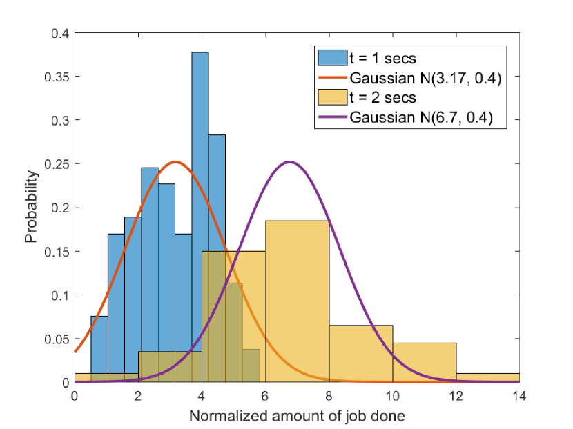
Figure 3: The distribution of the number of jobs completed by a given time.

We need to determine the probability that the master receives $k$ distinct blocks by time $t$ (so that the overall job has completed by time $t$). Let us define the random variable $Z_{t}$ to be

$$Z_{t}=\sum_{i=1}^{n}V_{i}^{t}.$$ (5)

As the workers are assumed to be independent, the number of jobs completed by the workers are also jointly independent and therefore $Z_{t}$ is a sum of independent discrete Gaussian distribution, which is equal to a discrete Gaussian with distribution

$$p\left(z_{t}|z_{t}\in\left[L\right]\right)=\frac{1}{\sqrt{2\pi{\sigma_{z}^{t}}^{2}}}e^{-\frac{(z_{t}-\gamma_{z}^{t})^{2}}{2{\sigma_{z}^{t}}^{2}}}$$ (6)

where

$$\gamma_{z}^{t}=\sum_{i=1}^{n}\frac{\gamma_{i}^{t}}{c_{i}},\ \ {\rm and}\ \ \sigma_{z}^{t}=\sqrt{\left(\sum_{i=1}^{n}{\frac{{\sigma_{i}^{t}}^{2}}{{c_{i}}^{2}}}\right)}.$$

We can now find the probability that the master node is able to collect $k$ distinct blocks by time $t$:

$$\text{Pr}[Z_{t}\geq k]=\sum_{z_{t}=k}^{L}p_{i}(z_{t}|z_{t}\in\mathbb{Z}).$$ (7)

In contrast to our approach, the lack of sub-blocking in the earlier literature [1, 5] restricted the $V_{i}^{t}$ to be in the set $\{0,l_{i}\}$. The option for the $V_{i}^{t}$ to take on a larger set of values gives our scheme a material advantage.

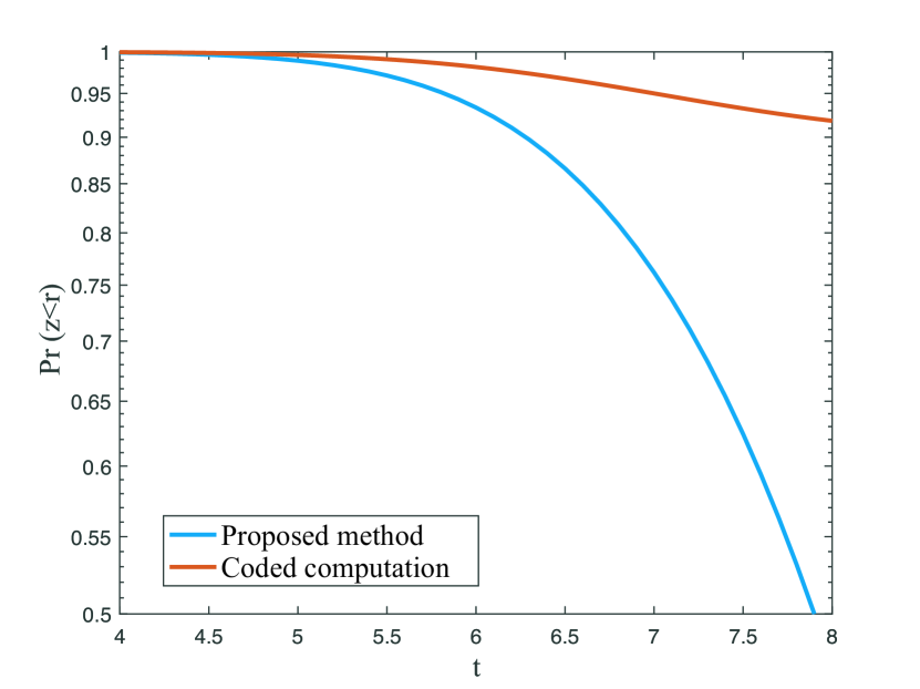
Figure 4: The probably of non-completion by a given time versus $t$, $\text{Pr}[Z_{t}<k]$.

Fig. 4 plots the probability that the master node does not acquire at least $k$ blocks as a function of time, i.e, $\text{Pr}[Z_{t}<k]=1-\text{Pr}[Z_{t}\geq k]$. This figure plots (7) when $m=1000,n=10,L=100,k=40,\gamma_{i}^{t}=0.5t$ and $\sigma_{i}^{t}=2$. It can be observed that, in our proposed scheme, the probability of not finishing the computation task by time $t$ decays much more quickly than for the scheme of [1].

V Numerical Evaluation

In this section several Monte Carlo simulations are presented to estimate the finishing time of different schemes. We compare our proposed scheme that exploits stragglers to the frequently-used approach of completely ignoring stragglers. In each trial of our simulations we generate $N$ independent exponential random numbers with mean $\frac{1}{\lambda}=1$. These $N$ numbers are denoted by $T_{1},T_{2},\ldots,T_{N}$, i.e., $T_{i}$ is the time to complete all subtasks. We consider $\frac{jT_{i}}{r^{2}}$ as the finishing time of the $j-$th subtask of the $i-$th processor where $j\in\{1,2,3,\ldots,r^{2}\}$ and $i\in\{1,2,3,\ldots,N\}$. In all simulations we set $k=20$.

Figure 5: The expected finishing time $E(T)$ vs. number of processors ($N$) for different number of subtasks ($r^{2}$).

In Fig. 5 the expected finishing times of the multiple ($\frac{N}{k}\times r$, $k\times r$) MDS-coded, ($\lfloor\sqrt{N}\rfloor\times r$, $k\times r$)² product-coded, and single ($N\times r^{2}$, $(k\times r)^{2}$) MDS-coded schemes are plotted for $N\in\{600,800,1000,...,2400\}$. We plotted results for both $r=1$ (equivalent to [1, 3]) and $r=2$. Fig. 5 shows that our method significantly reduces the finishing time. The gain is a result of increasing $r=1$ to $r=2$ such that each worker computes $r^{2}=4$ subtasks sequentially rather than $r^{2}=1$ (big) subtask as in [3].

Figure 6: The ratio of expected times of our scheme at $r=4$ to [3] vs. the number of processors ($N$).

The ratio of improvement between $r=1$ and $r=4$ is depicted in Fig. 6 for $N\in\{600,800,1000,...,2400\}$. Fig. 6 shows that by dividing the main task into $r^{2}=16$ subtasks is at least twice as good as compared to $r=1$ [3] and reaches three times for larger number of workers.

The impact of increasing $r$ on the average finishing time is shown in Fig. 7. The improvement from $r=1$ to $r=2$ is significant. For $r>4$ the further improvement, while positive, is not very significant. Therefore, excessively increasing in the number of subtasks is not logical due to the additive complexity incurred.

Fig. 8 illustrates the average finishing time when the order of processing is changed. In this figure we set $N=600$ and vary $r\in\{1,2,3,...,8\}$. It is observed in Fig. 8 that diagonal order of processing closely matches the random ordering. Further, column-wise (or row-wise) processing order is a bad choice.

Figure 7: The expected finishing time $E(T)$ vs. $r$ for $N=600$ processors.

Figure 8: The expected finishing time $E(T)$ vs. $r$ for different processing orders. We fixed $N=600$.

VI Conclusion

In this paper we have proposed a method to exploit the work completed by stragglers in distributed coded computation. We first applied our method to vector-matrix multiplication based on MDS codes. The main idea is to assign a large number of small MDS-coded jobs to workers, rather than to assign each worker a single (larger) job. By allowing workers to work on small jobs, workers can transmit back each partial solution as they complete each small job. Through these changes, we realize significant acceleration in comparison to previous approaches. We then extend our work to matrix-matrix multiplication. By selecting a suitable order of processing we achieved additional improvement in finishing time. We analyzed our scheme for MDS coded vector-matrix multiplication. The simulations show more than a factor of two improvement in the expected finishing time.

References

- [1] K. Lee, M. Lam, R. Pedarsani, D. Papailiopoulos, and K. Ramchandran, “Speeding up distributed machine learning using codes,” in IEEE Int. Symp. Inf. Theory (ISIT), July 2016, pp. 1143–1147.
- [2] S. Li, M. A. Maddah-Ali, and A. S. Avestimehr, “A unified coding framework for distributed computing with straggling servers,” in IEEE Globecom Workshops (GC Wkshps), Dec 2016, pp. 1–6.
- [3] K. Lee, C. Suh, and K. Ramchandran, “High-dimensional coded matrix multiplication,” in IEEE Int. Symp. Inf. Theory (ISIT), June 2017, pp. 2418–2422.
- [4] N. S. Ferdinand and S. C. Draper, “Anytime coding for distributed computation,” in Allerton Conf. on Commun., Control, and Comp., Sept 2016, pp. 954–960.
- [5] A. Reisizadeh, S. Prakash, R. Pedarsani, and S. Avestimehr, “Coded computation over heterogeneous clusters,” in IEEE Int. Symp. Inf. Theory (ISIT), June 2017, pp. 2408–2412.
- [6] S. Dutta, V. Cadambe, and P. Grover, “Coded convolution for parallel and distributed computing within a deadline,” in 2017 IEEE Int. Symp. on Inf. Theory (ISIT), June 2017, pp. 2403–2407.
- [7] R. Tandon, Q. Lei, A. G. Dimakis, and N. Karampatziakis, “Gradient Coding: Avoiding Stragglers in Distributed Learning,” in Proc. Int. Conf. on Machine Learning, 2017.
- [8] R. Roth, Introduction to Coding Theory. New York, NY, USA: Cambridge University Press, 2006.