Local chiral interactions, the tritium Gamow-Teller matrix element, and the three-nucleon contact term

Abstract

The Gamow-Teller (GT) matrix element contributing to tritium $\beta$ decay is calculated with trinucleon wave functions obtained from hyperspherical-harmonics solutions of the Schrödinger equation with the chiral two- and three-nucleon interactions including $\Delta$ intermediate states that have recently been constructed in configuration space. Predictions up to N3LO in the chiral expansion of the axial current (with $\Delta$’s) overestimate the empirical value by 1–4 %. By exploiting the relation between the low-energy constant (LEC) in the contact three-nucleon interaction and two-body axial current, we provide new determinations of the LECs $c_{D}$ and $c_{E}$ that characterize this interaction by fitting the trinucleon binding energy and tritium GT matrix element. Some of the implications that the resulting models of three-nucleon interactions have on the spectra of light nuclei and the equation of state of neutron matter are briefly discussed. We also provide a partial analysis, which ignores $\Delta$’s, of the contributions due to loop corrections in the axial current at N4LO. Finally, explicit expressions for the axial current up to N4LO have been derived in configuration space, which other researchers in the field may find useful.

I Introduction

Tritium $\beta$ decay and the Gamow-Teller (GT) matrix element contributing to it have provided, over the past several decades, a testing ground for models of the nuclear axial current and, in particular, for the role that many-body weak transition operators beyond the leading one-body GT operator play in this matrix element Chemtob:1969 ; Riska:1970 ; Fishbach:1972 ; Carlson:1991 ; Schiavilla:1998 as well as in the closely related one entering the cross section of the basic solar burning reaction ¹H$(p,e^{+}\nu_{e})^{2}$H Gari:1972 ; Dautry:1976 ; Carlson:1991 ; Schiavilla:1998 (in this connection, the first calculation of these processes in lattice quantum chromodynamics reported last year by the NPLQCD collaboration Savage:2017 should also be noted). More recently, the development of chiral effective field theory ($\chi$EFT) has led to a re-examination of these weak transitions within such a framework Park:1998 ; Park:2003 ; Marcucci:2013 ; Baroni:2016a ; Klos:2017 (as well as in formulations in which the pion degrees of freedom are integrated out—so called, pion-less effective field theory Butler:2001 ; De-Leon:2016 ). An important advantage of $\chi$EFT over older approaches based on meson-exchange phenomenology Chemtob:1971 ; Towner:1987 ; Riska:1989 has been in having established a relation between the three-nucleon ($3N$) interaction and the two-nucleon ($2N$) axial current Gardestig:2006 ; Gazit:2009 , specifically between the low-energy constant (LEC) $c_{D}$ (in standard notation) in the $3N$ contact interaction Epelbaum:2002 and the LEC in the $2N$ contact axial current Gazit:2009 . Thus, this makes it possible to use nuclear properties governed by either the strong or weak interactions to constrain simultaneously the $3N$ interaction and $2N$ axial current.

In this context, the present study addresses two topics. The first consists in an assessment of how well the experimental value of the ³H GT matrix element is reproduced in calculations based on nuclear Hamiltonians with the recently constructed chiral $2N$ and $3N$ interactions Piarulli:2016 ; Piarulli:2017 . These interactions, which are local in configuration space, have long-range parts mediated by one- and two-pion exchange (denoted as OPE and TPE, respectively), including $\Delta$-isobar intermediate states, up to next-to-next-to-leading order (N2LO) in the $2N$ case, and up to next-to-leading order (NLO) in the $3N$ case in the chiral expansion. The $2N$ and $3N$ short-range parts are parametrized by contact interactions up to, respectively, next-to-next-to-next-to-leading order (N3LO) Piarulli:2016 and NLO Piarulli:2017 . In particular, the LECs $c_{D}$ and $c_{E}$ which characterize the $3N$ contact terms have been fitted to the trinucleon binding energies and neutron-deuteron ($nd$) doublet scattering length. As shown below, the predicted GT matrix element with these interactions and accompanying axial currents is a few % larger than the empirical value.

The second topic deals with a determination of $c_{D}$ and $c_{E}$ in which we fit, rather than the scattering length, the ³H GT matrix element. Because of the much reduced correlation between binding energies and the GT matrix element, this procedure leads to a more robust determination of $c_{D}$ and $c_{E}$ than attained in the previous fit. The axial current here includes OPE terms with $\Delta$ intermediate states up to N3LO in the chiral counting of Ref. Baroni:2016 . The resulting values of $c_{D}$ and $c_{E}$ are rather different from those obtained earlier Piarulli:2017 , and the implications that these newly calibrated models of the $3N$ interaction have on the spectra of light nuclei and the equation of state of neutron matter are currently being investigated Piarulli:2018 (note that an error in the relation given in the original Ref. Gazit:2009 between the contact-axial-current LEC and $c_{D}$ has been corrected Schiavilla:2017 ).

Related issues which we also explore in this work are (i) the magnitude of contributions to the axial current beyond N3LO owing to loop corrections induced by TPE, and (ii) the extent to which these contributions impact the ³H GT matrix element and, in particular, modify the values of $c_{D}$ and $c_{E}$. Since currently available derivations of TPE axial currents in $\chi$EFT Baroni:2016 ; Krebs:2017 do not explicitly include $\Delta$’s, our comments regarding these two questions should be viewed, at this stage, as preliminary. Nevertheless, we believe that, even within the context of such an incomplete analysis, it is possible to draw some conclusions, especially in reference to the convergence pattern of the chiral expansion for the axial current.

This paper is organized as follows. In Sec. II we list explicit expressions in configuration space for the axial current up to N3LO. While these are well known Park:2003 , they are reported here for completeness and clarity of presentation, particularly in view of the regularization scheme in configuration space that has been adopted for consistency with the chiral interactions of Refs. Piarulli:2016 ; Piarulli:2015 . In Sec. III we present predictions for the ³H GT matrix element obtained with the LECs $c_{D}$ and $c_{E}$ of Ref. Piarulli:2017 , and in Sec. IV report a new set of values for these LECs resulting from fitting the GT matrix element and ³H/³He binding energies. In Sec. V we provide configuration-space expressions for the loop corrections of the axial current at N4LO Baroni:2016 ; Krebs:2017 , and estimates of their contributions. The actual derivation of these expressions, which to the best of our knowledge were previously not known, is relegated in Appendix A; the resulting N4LO current has a simple structure, which we hope will encourage its use by other researchers in the field. Finally, we offer some concluding remarks in Sec. VI.

II Axial currents up to N3LO in configuration space

We illustrate in Fig. 1 the contributions to the axial current in a $\chi$EFT with nucleon, $\Delta$-isobar, and pion degrees of freedom up to N3LO. Momentum-space expressions for panels (a) and (b), (c) and (d), (i) and (j), and (k) and (l) are listed in Ref. Baroni:2016 , respectively in Eqs. (3.14), (5.1)–(5.2), (5.5)–(5.6), and (5.4); the contributions of panels (g) and (h) vanish, while those of panels (e) and (f) read

$${\bf j}_{5,a}^{\rm N2LO}(\Delta)={\bf j}_{5,a}^{\Delta}-\frac{\bf q}{q^{2}+m_{\pi}^{2}}\,{\bf q}\cdot{\bf j}_{5,a}^{\Delta}\ ,$$ (1)

where

$${\bf j}_{5,a}^{\Delta} = \frac{g_{A}}{2\,f_{\pi}^{2}}\Big{[}2\,c^{\Delta}_{3}\,\tau_{j,a}\,{\bf k}_{j}+c^{\Delta}_{4}\,\left({\bm{\tau}}_{i}\times{\bm{\tau}}_{j}\right)_{a}{\bm{\sigma}}_{i}\times{\bf k}_{j}\Big{]}$$ (2)

$$\qquad\times\,{\bm{\sigma}}_{j}\cdot{\bf k}_{j}\,\frac{1}{\omega_{j}^{2}}+\left(i\rightleftharpoons j\right)\ ,$$

with the LECs $c_{3}^{\Delta}$ and $c_{4}^{\Delta}$ given by

$$c_{3}^{\Delta}=-\frac{h_{A}^{2}}{9\,m_{\Delta N}}\ ,\qquad c_{4}^{\Delta}=\frac{h_{A}^{2}}{18\,m_{\Delta N}}\ .$$ (3)

Here $g_{A}$ and $h_{A}$ are nucleon and nucleon-to-$\Delta$ axial coupling constants ($g_{A}\,$=$\,1.2723$ and $h_{A}\,$=$\,2.74$), $f_{\pi}$ and $m_{\Delta N}$ are the pion-decay constant and $\Delta$-nucleon mass difference ($f_{\pi}\,$=$\,92.4$ MeV and $m_{\Delta N}\,$=$\,293.1$ MeV), ${\bm{\sigma}}_{i}$ and ${\bm{\tau}}_{i}$ are the spin and isospin Pauli matrices of nucleon $i$, ${\bf p}_{i}$ and ${\bf p}^{\prime}_{i}$ are its initial and final momenta with the pion energy $\omega_{i}$ and pion momentum ${\bf k}_{i}$ defined as $\omega_{i}\,$=$\,\sqrt{k_{i}^{2}+m_{\pi}^{2}}$ and ${\bf k}_{i}\,$=$\,{\bf p}_{i}^{\prime}-{\bf p}_{i}$, and ${\bf k}_{i}+{\bf k}_{j}\,$=$\,{\bf q}$, where ${\bf q}$ is the external field momentum.

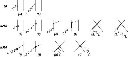
Figure 1: Diagrams illustrating the contributions to the axial current up to N3LO ($Q^{0}$). Nucleons, $\Delta$-isobars, pions, and external fields are denoted by solid, thick-solid, dashed, and wavy lines, respectively. The squares in panel (c) and (d) represent relativistic corrections, while the dots in panels (i) and (j) denote vertices implied by the ${\cal L}^{(2)}_{\pi N}$ chiral Lagrangian. Only a single time ordering is shown. Note that the contact contributions in panels (g) and (h) vanish.

We provide below the configuration-space expressions for these currents, ignoring pion-pole terms which contribute negligibly to the observable under consideration in the present work. The LO term, which scales as $Q^{-3}$ in the power counting ($Q$ denotes generically a low-momentum scale), reads

$${\bf j}^{\rm LO}_{5,a}({\bf q})=-\frac{g_{A}}{2}\,\tau_{i,a}\,{\bm{\sigma}}_{i}\,{\rm e}^{i{\bf q}\cdot{\bf r}_{i}}+(i\rightleftharpoons j)\ ,$$ (4)

while the N2LO and N3LO terms (scaling, respectively, as $Q^{-1}$ and $Q^{0}$) are written as

$${\bf j}^{\rm N2LO}_{5,a}({\bf q}) = {\bf j}^{\rm N2LO}_{5,a}({\bf q};{\rm RC})+{\bf j}^{\rm N2LO}_{5,a}({\bf q};\Delta)\ ,$$ (5)

$${\bf j}^{\rm N3LO}_{5,a}({\bf q}) = {\bf j}^{\rm N3LO}_{5,a}({\bf q};{\rm OPE})+{\bf j}^{\rm N2LO}_{5,a}({\bf q};{\rm CT})\ ,$$ (6)

where

$${\bf j}^{\rm N2LO}_{5,a}({\bf q};{\rm RC}) = \frac{g_{A}}{8\,m^{2}}\,\tau_{i,a}\left\{{\bf p}_{i}\times\left({\bm{\sigma}}_{i}\times{\bf p}_{i}\right)\,\,,\,\,{\rm e}^{i{\bf q}\cdot{\bf r}_{i}}\right\}+\frac{g_{A}}{8\,m^{2}}\,\tau_{i,a}\,{\rm e}^{i{\bf q}\cdot{\bf r}_{i}}\left(i\,{\bf q}\times{\bf p}_{i}+{\bf q}\,\,{\bm{\sigma}}_{i}\cdot{\bf q}/2\right)+(i\rightleftharpoons j)\ ,$$ (7)

$${\bf j}^{\rm N2LO}_{5,a}({\bf q};\Delta) = -{\rm e}^{i\,{\bf q}\cdot{\bf r}_{i}}\,\left({\bm{\tau}}_{i}\times{\bm{\tau}}_{j}\right)_{a}\left[I^{(1)}(\mu_{ij};\alpha_{1}^{\Delta})\,{\bm{\sigma}}_{i}\times{\bm{\sigma}}_{j}+I^{(2)}(\mu_{ij};\alpha_{1}^{\Delta})\,{\bm{\sigma}}_{i}\times\hat{\bf r}_{ij}\,\,{\bm{\sigma}}_{j}\cdot\hat{\bf r}_{ij}\right]$$ (8)

$$-\,{\rm e}^{i{\bf q}\cdot{\bf r}_{i}}\,\tau_{j,a}\left[I^{(1)}(\mu_{ij};\alpha_{2}^{\Delta})\,{\bm{\sigma}}_{j}+I^{(2)}(\mu_{ij};\alpha_{2}^{\Delta})\,\hat{\bf r}_{ij}\,\,{\bm{\sigma}}_{j}\cdot\hat{\bf r}_{ij}\right]+(i\rightleftharpoons j)\ ,$$

and

$${\bf j}^{\rm N3LO}_{5,a}({\bf q};{\rm OPE}) = -{\rm e}^{i\,{\bf q}\cdot{\bf r}_{i}}\,\left({\bm{\tau}}_{i}\times{\bm{\tau}}_{j}\right)_{a}\left[I^{(1)}(\mu_{ij};\alpha_{1})\,{\bm{\sigma}}_{i}\times{\bm{\sigma}}_{j}+I^{(2)}(\mu_{ij};\alpha_{1})\,{\bm{\sigma}}_{i}\times\hat{\bf r}_{ij}\,\,{\bm{\sigma}}_{j}\cdot\hat{\bf r}_{ij}\right]$$ (9)

$$-\,{\rm e}^{i{\bf q}\cdot{\bf r}_{i}}\,\tau_{j,a}\left[I^{(1)}(\mu_{ij};\alpha_{2})\,{\bm{\sigma}}_{j}+I^{(2)}(\mu_{ij};\alpha_{2})\,\hat{\bf r}_{ij}\,\,{\bm{\sigma}}_{j}\cdot\hat{\bf r}_{ij}\right]$$

$$-\left({\bm{\tau}}_{i}\times{\bm{\tau}}_{j}\right)_{a}\,\frac{1}{2\,m_{\pi}}\left\{{\bf p}_{i}\,\,,\,\,{\rm e}^{i{\bf q}\cdot{\bf r}_{i}}\,\widetilde{I}^{\,(1)}(\mu_{ij};\widetilde{\alpha}_{1})\,{\bm{\sigma}}_{j}\cdot\hat{\bf r}_{ij}\right\}$$

$$-i\,\left({\bm{\tau}}_{i}\times{\bm{\tau}}_{j}\right)_{a}\,{\rm e}^{i{\bf q}\cdot{\bf r}_{i}}\,\widetilde{I}^{\,(1)}(\mu_{ij};\widetilde{\alpha}_{2})\,{\bm{\sigma}}_{i}\times\frac{{\bf q}}{m_{\pi}}\,\,{\bm{\sigma}}_{j}\cdot\hat{\bf r}_{ij}+(i\rightleftharpoons j)\ ,$$

$${\bf j}^{\rm N3LO}_{5,a}({\bf q};{\rm CT}) = z_{0}\,{\rm e}^{i\,{\bf q}\cdot{\bf R}_{ij}}\,\frac{{\rm e}^{-z_{ij}^{2}}}{\pi^{3/2}}\,\left({\bm{\tau}}_{i}\times{\bm{\tau}}_{j}\right)_{a}\,\left({\bm{\sigma}}_{i}\times{\bm{\sigma}}_{j}\right)\ ,$$ (10)

and ${\bf p}_{k}\,$=$\,-i\,{\bm{\nabla}}_{k}$ is the momentum operator of nucleon $k$, $\left\{\dots\,,\,\dots\right\}$ denotes the anticommutator,

$${\bf r}_{ij} = {\bf r}_{i}-{\bf r}_{j}\ ,\qquad{\bf R}_{ij}=\left({\bf r}_{i}+{\bf r}_{j}\right)/2\ ,$$ (11)

$$\qquad\mu_{ij} = m_{\pi}r_{ij}\ ,\qquad z_{ij}=r_{ij}/R_{\rm S}\ ,$$ (12)

and the $\delta$-function in the contact axial current has been smeared by replacing it with a Gaussian cutoff of range $R_{\bf S}$ Piarulli:2015 ; Piarulli:2016 . The adimensional LEC $z_{0}$ is given by

$$z_{0} = \frac{g_{A}}{2}\,\frac{m_{\pi}^{2}}{f_{\pi}^{2}}\,\frac{1}{\left(m_{\pi}\,R_{\rm S}\right)^{3}}\bigg{[}-\frac{m_{\pi}}{4\,g_{A}\,\Lambda_{\chi}}\,c_{D}$$ (13)

$$+\frac{m_{\pi}}{3}\left(c_{3}+c_{3}^{\Delta}+2\,c_{4}+2\,c_{4}^{\Delta}\right)+\frac{m_{\pi}}{6\,m}\bigg{]}\ ,$$

where $c_{D}$ denotes the LEC multiplying one of the contact terms in the three-nucleon interaction Epelbaum:2002 , and it should be noted that the combination $c_{3}^{\Delta}+2\,c_{4}^{\Delta}$ vanishes. It has recently been realized Schiavilla:2017 that the relation between $z_{0}$ and $c_{D}$ had been given erroneously in the original reference Gazit:2009 , a – sign and a factor 1/4 were missing in the term proportional to $c_{D}$. The various correlation functions are defined as

$$I^{(1)}(\mu;\alpha) = -\alpha\,(1+\mu)\,\frac{e^{-\mu}}{\mu^{3}}\ ,$$ (14)

$$I^{(2)}(\mu;\alpha) = \alpha\,(3+3\,\mu+\mu^{2})\,\frac{e^{-\mu}}{\mu^{3}}\ ,$$ (15)

$$\widetilde{I}^{\,(1)}(\mu;\widetilde{\alpha}) = -\widetilde{\alpha}\,(1+\mu)\,\frac{e^{-\mu}}{\mu^{2}}\ ,$$ (16)

where

$$\!\!\!\!\!\!\!\!\alpha_{1}^{\Delta} = \frac{g_{A}}{8\,\pi}\,\frac{m_{\pi}^{3}}{f_{\pi}^{2}}\,c_{4}^{\Delta}\ ,\,\,\,\alpha_{2}^{\Delta}=\frac{g_{A}}{4\,\pi}\,\frac{m_{\pi}^{3}}{f_{\pi}^{2}}\,c_{3}^{\Delta}\ ,$$ (17)

$$\!\!\!\!\!\!\!\!\alpha_{1} = \frac{g_{A}}{8\,\pi}\,\frac{m_{\pi}^{3}}{f_{\pi}^{2}}\left(c_{4}+\frac{1}{4\,m}\right)\ ,\,\,\,\alpha_{2}=\frac{g_{A}}{4\,\pi}\,\frac{m_{\pi}^{3}}{f_{\pi}^{2}}\,c_{3}\ ,$$ (18)

$$\!\!\!\!\!\!\!\!\widetilde{\alpha}_{1} = \frac{g_{A}}{16\,\pi}\,\frac{m_{\pi}^{3}}{m\,f_{\pi}^{2}}\ ,\,\,\,\widetilde{\alpha}_{2}=\frac{g_{A}}{32\,\pi}\,\frac{m_{\pi}^{3}}{m\,f_{\pi}^{2}}\left(c_{6}+1\right)\ ,$$ (19)

$m_{\pi}$ and $m$ are the pion and nucleon masses, $\Lambda_{\chi}\,$=$\,1$ GeV, and the LECs $c_{3}$, $c_{4}$, and $c_{6}$ have the values Piarulli:2015 ; Krebs:2007

$$c_{3}=-0.79\,\,{\rm GeV}^{-1}\ ,\,\,c_{4}=1.33\,\,\,{\rm GeV}^{-1}\ ,\,\,\,c_{6}=5.83\ .$$ (20)

Each correlation function above is regularized by multiplication of a configuration-space cutoff as in the case of the local chiral potentials of Refs. Piarulli:2015 ; Piarulli:2016 , namely

$$X^{(1,2)}(m_{\pi}r)\longrightarrow C_{R_{\rm L}}(r)\,X^{(1,2)}(m_{\pi}r)$$ (21)

with

$$C_{R_{\rm L}}(r)=1-\frac{1}{\left(r/R_{\rm L}\right)^{p}\,{\rm e}^{(r-R_{\rm L})/a_{\rm L}}+1}\ ,$$ (22)

where $a_{\rm L}\,$=$\,R_{\rm L}/2$, the exponent $p$ is taken as $p\,$=$\,6$, and $X$ stands for $I$ or $\widetilde{I}$. Finally, charge-raising ($+$) or charge-lowering ($-$) currents are obtained from ${\bf j}_{5,\pm}={\bf j}_{5,x}\pm i\,{\bf j}_{5,y}$, and hereafter, we define the isospin combinations

$$\tau_{i,\pm} = (\tau_{i,x}\pm i\,\tau_{i,y})/2\ ,$$ (23)

$$({\bm{\tau}}_{1}\times{\bm{\tau}}_{2})_{\pm} = ({\bm{\tau}}_{1}\times{\bm{\tau}}_{2})_{x}\pm i\,({\bm{\tau}}_{1}\times{\bm{\tau}}_{2})_{y}\ .$$ (24)

III ³H $\beta$ decay with local chiral interactions

In recent years, local chiral $2N$ interactions have been derived Gezerlis:2013 ; Piarulli:2015 ; Piarulli:2016 in configuration space, primarily for use in quantum Monte Carlo calculations of light-nuclei and neutron-matter properties Gezerlis:2014 ; Lynn:2014 ; Lynn:2016 ; Tews:2016 ; Gandolfi:2017 ; Lynn:2017 ; Piarulli:2017 . Here we focus on the family of interactions constructed by our group Piarulli:2016 . These are written as the sum of an electromagnetic-interaction component, including up to quadratic terms in the fine-structure constant, and a strong-interaction component characterized by long- and short-range parts. The long-range part includes OPE and TPE terms up to N2LO in the chiral expansion Piarulli:2015 , derived in the static limit from leading and sub-leading $\pi N$ and $\pi N\Delta$ chiral Lagrangians. In coordinate space, this long-range part is represented by charge-independent central, spin, and tensor components with and without isospin dependence ${\bm{\tau}}_{i}\cdot{\bm{\tau}}_{j}$ (the so-called $v_{6}$ operator structure), and by charge-independence-breaking central and tensor components induced by OPE and proportional to the isotensor operator $T_{ij}\,$=$\,3\,\tau^{z}_{i}\,\tau^{z}_{j}-{\bm{\tau}}_{i}\cdot{\bm{\tau}}_{j}$. The radial functions multiplying these operators are singular at the origin, and are regularized by a cutoff of the form given in Eq. (22).

The short-range part is described by charge-independent contact interactions up to N3LO, specified by a total of 20 LECs, and charge-dependent ones up to NLO, characterized by 6 LECs Piarulli:2016 . By utilizing Fierz identities, the resulting charge-independent interaction can be made to contain, in addition to the $v_{6}$ operator structure, spin-orbit, ${\bf L}^{2}$ (${\bf L}$ is the relative orbital angular momentum), and quadratic spin-orbit components, while the charge-dependent one retains central, tensor, and spin-orbit components. Both are regularized by multiplication of a Gaussian cutoff $C_{R_{\rm S}}(r)\,$= $\,{\rm exp}\left[-(r/R_{\rm S})^{2}\right]/\left(\pi^{3/2}R_{\rm S}^{3}\right)$, as in the contact axial current, Eq. (10).

Two classes of interactions were constructed, which only differ in the range of laboratory energy over which the fits to the $2N$ database Perez:2013 were carried out, either 0–125 MeV in class I or 0–200 MeV in class II. For each class, three different sets of cutoff radii $(R_{\rm S},R_{\rm L})$ were considered $(R_{\rm S},R_{\rm L})\,$=$\,(0.8,1.2)$ fm in set a, (0.7,1.0) fm in set b, and (0.6,0.8) fm in set c. The $\chi^{2}$/datum achieved by the fits in class I (II) was $\lesssim 1.1$ $(\lesssim 1.4)$ for a total of about 2700 (3700) data points. We have been referring to these high-quality $2N$ interactions generically as the Norfolk $v_{ij}$’s (NV2s), and have been designating those in class I as NV2-Ia, NV2-Ib, and NV2-Ic, and those in class II as NV2-IIa, NV2-IIb, and NV2-IIc. Owing to the poor convergence of the hyperspherical-harmonics (HH) expansion and the severe fermion-sign problem of the Green function Monte Carlo (GFMC) method, however, models Ic and IIc have not been used (at least, not yet) in actual calculations of light nuclei.

The NV2s were found to underbind, in GFMC calculations, the ground-state energies of nuclei with $A\,$=$\,3$–6 Piarulli:2016 . To remedy this shortcoming, in Ref. Piarulli:2017 we constructed the leading $3N$ interaction in a $\chi$EFT, including $\Delta$ intermediate states. It consists Epelbaum:2002 of a long-range piece mediated by TPE at LO and NLO, and a short-range piece parametrized in terms of two contact interactions, which enter formally at NLO. The two (adimensional) LECs $c_{D}$ and $c_{E}$, which characterize these latter interactions, were determined in HH calculations by simultaneously reproducing the experimental trinucleon ground-state energies and the $nd$ doublet scattering length for each of the $2N$ models considered, namely, Ia and Ib, and IIa and IIb. It was then shown Piarulli:2017 that the Hamiltonian based on the interactions NV2+3-Ia led, in GFMC calculations, to an excellent description of the spectra of light nuclei in the mass range $A\,$=$\,4$–12, including their level ordering and spin-orbit splittings. It has since become clear Piarulli:2018 that the other models (NV2+3-Ib, etc.) do not provide a description of these spectra as satisfactory as that obtained with NV2+3-Ia.

Given the value of $c_{D}$, the axial current is fully constrained, since the LEC $z_{0}$ in the contact term is fixed via Eq. (13). The evaluation of the tritium Gamow-Teller (GT) matrix element is carried out by Monte Carlo integration Baroni:2016a , and statistical errors are less than a % for each individual contribution (in fact, at the level of a few parts in $10^{-4}$ for the LO). Predictions obtained with the Hamiltonian models NV2+3-Ia/b and NV2+3-IIa/b and at vanishing momentum transfer (${\bf q}\,$=$\,0$) are reported in Table 1. The experimental value, as obtained in the analysis of Ref. Baroni:2016a , is ${\rm GT}_{\rm exp}\,$=$\,0.9511\pm 0.0013$; it is underestimated at LO by all models at the 3% level, but is overestimated by $\lesssim\,$4% in the N3LO calculations. As it can be surmised from the difference between models a and b in both classes I and II, the LO contribution is very weakly dependent on the pair of cutoff radii ($R_{\rm S}$,$R_{\rm L}$), characterizing the two- and three-nucleon interactions from which the ³H and ³He HH wave functions are derived. In contrast, the cutoff dependence is much more pronounced in the case of the N2LO and N3LO contributions, since for these the short- and long-range regulators directly enter the correlation functions of the corresponding transition operators. The N2LO(RC) correction, which is nominally suppressed by two powers of the expansion parameter $Q/\Lambda_{\chi}$, being inversely proportional to the square of the nucleon mass, itself of order $\Lambda_{\chi}$, is in fact further suppressed than the naive N2LO power counting would imply. Indeed, it is almost an order of magnitude smaller, and of opposite sign, than the N2LO($\Delta$) contribution.

	Ia	Ib	IIa	IIb
$c_{D}$	$3.666$	$-2.061$	$1.278$	$-4.480$
$c_{E}$	$-1.638$	$-0.982$	$-1.029$	$-0.412$
LO	$0.9248$	$0.9237$	$0.9249$	$0.9259$
N2LO($\Delta$)	$0.0401$	$0.0586$	$0.0406$	$0.0589$
N2LO(RC)	$-0.0055$	$-0.0063$	$-0.0059$	$-0.0077$
N3LO(OPE)	$0.0327$	$0.0457$	$0.0330$	$0.0462$
N3LO(CT)	$-0.0036$	$-0.0487$	$-0.0249$	$-0.0668$
TOT	$0.9885$	$0.9730$	$0.9677$	$0.9565$

Table 1: Contributions to the GT matrix element in tritium $\beta$ decay obtained with chiral axial currents up to N3LO and HH wave functions corresponding to the NV2+3-Ia/b and NV2+3-IIa/b chiral Hamiltonians. The experimental value is $0.9511\pm 0.0013$ Baroni:2016a , to be compared to the sum of these contributions (row labeled TOT). Also listed are the $c_{D}$ and $c_{E}$ values of the contact terms in the three-nucleon interactions of these Hamiltonians Piarulli:2017 .

The sum of the N2LO($\Delta$) and N3LO(OPE) contributions in Table 1 should be compared to the N3LO(OPE) contribution reported in Ref. Baroni:2016a for the combinations of the Entem and Machleidt (momentum-space) $2N$ interactions at N3LO Entem:2003 ; Machleidt:2011 and the Epelbaum et al. $3N$ interactions at LO Epelbaum:2002 (i.e., the TPE piece proportional to $c_{1}$, $c_{3}$, and $c_{4}$, and the $c_{D}$ and $c_{E}$ contact terms). In that work, $\Delta$-isobar degrees of freedom were included implicitly, as reflected by the much larger values (in magnitude) considered for the LECs $c_{3}$ and $c_{4}$. We found in Ref. Baroni:2016a the N3LO(OPE) contribution to be 0.0082 (0.00043) or 0.0579 (0.0652) with the momentum-space cutoff $\Lambda\,$=$\,500\,\,(600)$ MeV depending on which $c_{3}$-$c_{4}$ set was used, either the values reported by Entem and Machleidt Machleidt:2011 in the first case or the recent determinations by Hoferichter and collaborators Hoferichter:2015 in the second case. Here, we obtain values in the range 0.073–0.104, the lower (upper) limit corresponding to models a (b). As we noted in Ref. Baroni:2016a , there are cancellations between the individual terms proportional to $c_{3}$ and $c_{4}$, which make their sum very sensitive to the actual values adopted for these LECs. Nevertheless, it would appear that the present results are close to those obtained in that work with the $c_{3}$ and $c_{4}$ values from Ref. Hoferichter:2015 .

The magnitude (and sign) of the N3LO(CT) contribution results from the product of the matrix element

$$\sum_{i\leq j}\,\langle^{3}{\rm He}|\,{\rm e}^{-z_{ij}^{2}}\,\left({\bm{\tau}}_{i}\times{\bm{\tau}}_{j}\right)_{+}\left({\bm{\sigma}}_{i}\times{\bm{\sigma}}_{j}\right)_{z}|^{3}{\rm H}\rangle<0\ ,$$ (25)

and magnitude and sign of the LEC $z_{0}$, which is proportional to

$$z_{0} \propto -\frac{m_{\pi}}{4\,g_{A}\,\Lambda_{\chi}}\,c_{D}+\frac{m_{\pi}}{3}\left(c_{3}+2\,c_{4}\right)+\frac{m_{\pi}}{6\,m}$$ (26)

$$\simeq 0.1105-0.0271\,c_{D}\ .$$

For the $c_{D}$ values corresponding to the interactions NV2+3-Ia/b and NV2+3-IIa/b, we find that the N3LO(CT) contribution is negative overall. Because of the cancellation in $z_{0}$ between the constant term and the term proportional to $c_{D}$ in Eq. (26), its magnitude is accidentally very small for model Ia.

	Ia	Ib	IIa	IIb
CT1	$-0.0036$	$-0.0487$	$-0.0249$	$-0.0668$
CT2	$-0.0037$	$-0.0493$	$-0.0252$	$-0.0677$
CT3	$-0.0036$	$-0.0487$	$-0.0249$	$-0.0669$
CT4	$-0.0036$	$-0.0482$	$-0.0246$	$-0.0660$

Table 2: Contributions of four different parameterizations of the contact axial current to the GT matrix element in tritium. The first row is the same as listed in Table 1.

The N3LO(CT) contribution is only very marginally affected by the operator structure adopted for the contact axial current, more specifically

$$\!\!\!\!\!\!\!{\bf j}^{\rm N3LO}_{5,+}({\rm CT1}) = z_{0}\,\frac{{\rm e}^{-z_{ij}^{2}}}{\pi^{3/2}}\,\left({\bm{\tau}}_{i}\times{\bm{\tau}}_{j}\right)_{+}\,\left({\bm{\sigma}}_{i}\times{\bm{\sigma}}_{j}\right)\ ,$$ (27)

$$\!\!\!\!\!\!\!{\bf j}^{\rm N3LO}_{5,+}({\rm CT2}) = 4\,z_{0}\,\frac{{\rm e}^{-z_{ij}^{2}}}{\pi^{3/2}}\,\left({\bm{\sigma}}_{i}\,\tau_{i,+}+{\bm{\sigma}}_{j}\,\tau_{j,+}\right)\ ,$$ (28)

$$\!\!\!\!\!\!\!{\bf j}^{\rm N3LO}_{5,+}({\rm CT3}) = 2\,z_{0}\,\frac{{\rm e}^{-z_{ij}^{2}}}{\pi^{3/2}}\,\left({\bm{\sigma}}_{i}-{\bm{\sigma}}_{j}\right)\left(\tau_{i,+}-\tau_{j,+}\right)\ ,$$ (29)

$$\!\!\!\!\!\!\!{\bf j}^{\rm N3LO}_{5,+}({\rm CT4}) = -4\,z_{0}\,\frac{{\rm e}^{-z_{ij}^{2}}}{\pi^{3/2}}\,\left({\bm{\sigma}}_{i}\,\tau_{j,+}+{\bm{\sigma}}_{j}\,\tau_{i,+}\right)\ ,$$ (30)

where the isospin-raising operators are defined as in Eq. (23). These structures, which are Fierz-equivalent in the absence of the cutoff, are no longer so when the latter is included. The contributions corresponding to the set above are reported in Table 2.

IV Refitting $c_{D}$ with local chiral interactions

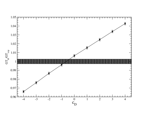
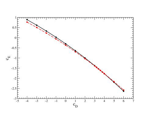
Figure 2: Upper panel: The calculated ratio GT_th/GT_exp as function of $c_{D}$ (solid line; each point on this line reproduces the trinucleon binding energies). Lower panel: The $c_{D}$-$c_{E}$ trajectories obtained by fitting the experimental trinucleon binding energies (solid line) and $nd$ doublet scattering length (dashed line) (the intercept of these two lines gives the $c_{D}$ and $c_{E}$ values that reproduce these two observables simultaneously). The NV2+3-Ia chiral interactions are used here for illustration. The values of 8.475 MeV and 7.725 MeV, and $0.645\pm 0.010$ fm Schoen:2003 are used for the ³H and ³He binding energies, and $nd$ scattering length, respectively. Note that these energies have been corrected for the small contributions ($+7$ keV in ³H and $-7$ keV in ³He) due to the $n$-$p$ mass difference Nogga:2003 . The band (left panel) results from experimental uncertainty GT_EXP, which has conservatively been doubled.

In this section, we determine the LECs $c_{D}$ and $c_{E}$ in the three-nucleon contact interaction, as parametrized in Ref. Piarulli:2017 , by fitting the experimental trinucleon binding energies and central value of the ³H GT matrix element. We designate these new LECs as $c_{D}^{*}$ and $c_{E}^{*}$. The fit is carried out as in Ref. Baroni:2016a ; Marcucci:2012 . We span a broad range of values in $c_{D}$, and, in correspondence to each $c_{D}$ in this range, determine $c_{E}$ so as to reproduce the binding energy of either ³H or ³He. The resulting trajectories are nearly indistinguishable Baroni:2016a ; Marcucci:2012 . Then, for each set of $(c_{D},c_{E})$, the triton and ³He wave functions are calculated and the GT matrix element, denoted as GT_th, is obtained, by including in the axial current contributions up to N3LO. The ratio GT_th/GT_exp for the case of the NV2+3-Ia interactions is shown in Fig. 2 (left panel), where the band reflects the uncertainty resulting from the experimental error on GT_exp, which, conservatively, has been doubled. The LECs $(c^{*}_{D},c^{*}_{E})$ that reproduce GT_exp (its central value) and the trinucleon binding energies are reported in Table 3, along with the axial current contributions at LO, N2LO, and N3LO. In Table 4, we provide the range of $(c_{D}^{*},c_{E}^{*})$ values compatible with the experimental error on GT_exp. The $3N$ interactions corresponding to the new set of $(c_{D}^{*},c_{E}^{*})$ are denoted with ^∗ hereafter.

	Ia∗	Ib∗	IIa∗	IIb∗
$c^{*}_{D}$	$-0.635$	$-4.71$	$-0.61$	$-5.25$
$c_{E}^{*}$	$-0.09$	$0.55$	$-0.35$	$0.05$
LO	$0.9272$	$0.9247$	$0.9261$	$0.9263$
N2LO	$0.0345$	$0.0517$	$0.0345$	$0.0515$
N3LO(OPE)	$0.0327$	$0.0454$	$0.0330$	$0.0465$
N3LO(CT)	$-0.0435$	$-0.0715$	$-0.0432$	$-0.0737$

Table 3: The values $c^{*}_{D}$ and $c^{*}_{E}$ obtained by fitting the experimental trinucleon binding energies and central value of the ³H GT matrix element with chiral axial currents up to N3LO and HH wave functions corresponding to the NV2+3-Ia^∗/b^∗ and NV2+3-IIa^∗/b^∗ chiral Hamiltonians. Also reported are the contributions at LO, N2LO, N3LO(OPE), and N3LO(CT).

It is interesting to compare the present $(c_{D},c_{E})$ trajectories (left panel of Fig. 2) with those of Ref. Piarulli:2017 (right panel), obtained by fitting the experimental $nd$ doublet scattering length rather than GT_exp. The strategy adopted in the present work appears to be more robust than that of Ref. Piarulli:2017 , since there the strong correlation between binding energy and scattering length makes the simultaneous determination of $(c_{D},c_{E})$ problematic. This difficulty is removed here.

The most striking difference between the previous and present determinations of LECs is in the values of $c_{E}$ and $c_{E}^{*}$, in particular the fact that $c_{E}^{*}$ is quite small in magnitude and not consistently negative as obtained in Ref. Piarulli:2017 . A negative $c_{E}$ leads to a repulsive contribution for the associated three-nucleon contact interaction in light nuclei Piarulli:2017 , but to an attractive one in pure neutron matter. Indeed, auxiliary-field diffusion Monte Carlo (AFDMC) calculations show Piarulli:2018 that the large and negative $c_{E}$ value for model NV2+3-Ia ($c_{E}\,$=$\,-1.638$) turns out to be disastrous in neutron matter, since it leads to collapse already at moderate densities (at $\rho\,$$\simeq$$\,\rho_{0}\,$= 0.16 neutron/fm³). Thus, even though this model reproduces quite well the low-lying spectra of nuclei in the mass range $A\,$= 4–12, it cannot sustain the existence of neutron stars of twice solar masses, and is therefore at variance with recent observations Demorest:2010 ; Antoniadis:2013 . The present determinations (the $c^{*}_{E}$’s) will mitigate, if not resolve, this issue Piarulli:2018 . Furthermore, because of their smallness (in magnitude), they will very substantially reduce the cutoff dependence seen in AFDMC calculations of the neutron-matter equation of state at high densities Lynn:2016 . There are also first indications that these new models, NV2+3-Ia^∗/b^∗ and NV2+3-IIa^∗/b^∗, predict light-nuclei spectra in reasonable agreement with experimental data Piarulli:2018 .

There is a large variation between the $c_{D}^{*}$ values obtained with models NV2+3-Ia^∗/IIa^∗ and those with models NV2+3-Ib^∗/IIb^∗, which simply reflects the cutoff dependence of the N2LO($\Delta$), N3LO(OPE), and N3LO(CT) contributions (see Table 3). The cutoff radii $(R_{\rm S},R_{\rm L})$ are (0.8,1.2) fm for the former (a models) and (0.7,1.0) fm for the latter (b models). As a consequence, the N2LO($\Delta$) and N3LO(OPE) contributions, which both have the same (positive) sign, increase the LO contribution and lead to an overestimate of GT_exp. This offset is then corrected by the N3LO(CT) contribution. In contrast to the earlier fits Piarulli:2017 , we find the present determinations of $c^{*}_{D}$ to be consistently negative, which make the term in the three-nucleon contact interaction proportional to it repulsive in both light nuclei and nuclear and neutron matter. However, because of its one-pion leg, it is highly sensitive to tensor correlations induced by the $2N$ interaction, so its contribution in neutron matter, where such correlations are weak, is noticeably reduced.

	Ia∗	Ib∗	IIa∗	IIb∗
$c^{*}_{D}$	$(-0.89,-0.38)$	$(-4.99,-4.42)$	$(-0.89,-0.33)$	$(-5.56,-4.94)$
$c_{E}^{*}$	$(-0.01,-0.17)$	$(+0.70,+0.40)$	$(-0.25,-0.45)$	$(+0.23,-0.13)$

Table 4: The range of $c^{*}_{D}$ and $c^{*}_{E}$ values allowed by the experimental error on GT_exp (note that this error has conservatively been doubled). The lower/upper limits correspond to GT${}_{\rm exp}-\!/\!+$ error.

V Estimate of axial current contributions at N4LO

In this section, we provide estimates of N4LO corrections to the GT matrix element in ³H. These estimates are incomplete, since the calculations reported here ignore $\Delta$ intermediate states in the axial current at N4LO. We are not aware of formal derivations of the two-body (and three-body) axial currents at this order, which include, beyond nucleon and pion, explicit $\Delta$ degrees of freedom. Nevertheless, it is interesting to have an approximate estimate for the magnitude of the presently known N4LO corrections. As a by-product of this effort, we also obtain analytical expressions in configuration space for these corrections, which other researchers in the field may find useful.

The (static part of the) axial current at N4LO was given in the Baroni et al. papers and accompanying errata Baroni:2016a ; Baroni:2016 . It is written as the sum of three terms: the first (labeled OPE) represents loop corrections to the OPE axial current, the second (labeled TPE) represents genuine TPE contributions, and the last (labeled CT) includes contact contributions induced by the regularization scheme in configuration space we have adopted (see Appendix A for a discussion),

$${\bf j}_{5,a}^{\rm N4LO}({\bf q})={\bf j}^{\rm OPE}_{5,a}({\bf q})+{\bf j}^{\rm TPE}_{5,a}({\bf q})+{\bf j}_{5,a}^{\rm CT}({\bf q})\ ,$$ (31)

where

$${\bf j}_{5,a}^{\rm OPE}({\bf q}) = {\rm e}^{i{\bf q}\cdot{\bf r}_{i}}\,\frac{1}{9}\left({\bm{\tau}}_{i}\times{\bm{\tau}}_{j}\right)_{a}\left[I^{(1)}(\mu_{ij};\beta)\,{\bm{\sigma}}_{i}\times{\bm{\sigma}}_{j}+I^{(2)}(\mu_{ij};\beta)\,{\bm{\sigma}}_{i}\times\hat{\bf r}_{ij}\,\,{\bm{\sigma}}_{j}\cdot\hat{\bf r}_{ij}\right]$$ (32)

$$-{\rm e}^{i{\bf q}\cdot{\bf r}_{i}}\,\tau_{j,a}\left[I^{(1)}(\mu_{ij};\beta)\,{\bm{\sigma}}_{j}+I^{(2)}(\mu_{ij};\beta)\,\hat{\bf r}_{ij}\,\,{\bm{\sigma}}_{j}\cdot\hat{\bf r}_{ij}\right]+(i\rightleftharpoons j)\ ,$$

$${\bf j}_{5,a}^{\rm TPE}({\bf q}) = {\rm e}^{i{\bf q}\cdot{\bf r}_{i}}\,\tau_{j,a}\left[F^{(0)}_{1}(\lambda_{ij})\,{\bm{\sigma}}_{i}-F^{(1)}_{2}(\lambda_{ij})\,{\bm{\sigma}}_{i}-F^{(2)}_{2}(\lambda_{ij})\,\hat{\bf r}_{ij}\,{\bm{\sigma}}_{i}\cdot\hat{\bf r}_{ij}\right]-\,{\rm e}^{i{\bf q}\cdot{\bf r}_{i}}\,\tau_{i,a}\left[F^{(1)}_{3}(\lambda_{ij})\,{\bm{\sigma}}_{j}+F^{(2)}_{3}(\lambda_{ij})\,\hat{\bf r}_{ij}\,{\bm{\sigma}}_{j}\cdot\hat{\bf r}_{ij}\right]$$ (33)

$$\!\!\!\!\!-{\rm e}^{i\,{\bf q}\cdot{\bf R}_{ij}}\,\tau_{j,a}\left[G^{(0)}_{1}(\lambda_{ij})\,{\bm{\sigma}}_{j}+H_{1}^{(1)}(\lambda_{ij})\,{\bm{\sigma}}_{j}+H^{(2)}_{1}(\lambda_{ij})\,\hat{\bf r}_{ij}\,{\bm{\sigma}}_{j}\cdot\hat{\bf r}_{ij}\right]$$

$$\!\!\!\!\!+{\rm e}^{i\,{\bf q}\cdot{\bf R}_{ij}}\!\left({\bm{\tau}}_{i}\times{\bm{\tau}}_{j}\right)_{a}\!\left[H_{3}^{(1)}(\lambda_{ij})\,{\bm{\sigma}}_{i}\times{\bm{\sigma}}_{j}\!+\!H_{3}^{(2)}(\lambda_{ij})\,{\bm{\sigma}}_{i}\times\hat{\bf r}_{ij}\left({\bm{\sigma}}_{j}\cdot\hat{\bf r}_{ij}\right)\right]\!+\!(i\rightleftharpoons j),$$

$${\bf j}_{5,a}^{\rm CT}({\bf q}) = {\rm e}^{i\,{\bf q}\cdot{\bf R}_{ij}}\left({\bm{\tau}}_{i}\times{\bm{\tau}}_{j}\right)_{a}I^{(0)}(z_{ij};\infty)\,{\bm{\sigma}}_{i}\times{\bm{\sigma}}_{j}+\Big{[}{\rm e}^{i{\bf q}\cdot{\bf r}_{i}}\,\tau_{j,a}\,F^{(0)}_{1}(z_{ij};\infty)\,{\bm{\sigma}}_{i}$$ (34)

$$-{\rm e}^{i\,{\bf q}\cdot{\bf R}_{ij}}\,\tau_{j,a}\,G^{(0)}_{1}(z_{ij};\infty)\,{\bm{\sigma}}_{j}+(i\rightleftharpoons j)\Big{]}\ ,$$

and pion-pole contributions are provided in Appendix A for completeness. The various correlation functions, regularized by multiplication of configuration-space cutoffs as in Sec. II (and Refs. Piarulli:2015 ; Piarulli:2016 ), are listed in Eqs. (14)–(15) and Appendix A, Eqs. (83)–(92) and Eqs. (98)–(99); furthermore, we have defined

$$I^{(0)}(z_{ij};\infty)=\frac{5\,g_{A}^{5}}{1536\,\pi}\,\frac{m^{4}_{\pi}}{f_{\pi}^{4}}\,\frac{1}{\left(m_{\pi}R_{\rm S}\right)^{3}}\,\frac{{\rm e}^{-z_{ij}^{2}}}{\pi^{3/2}}\ ,$$ (35)

and

$$\beta=\frac{9\,g^{5}_{A}}{1024\,\pi^{2}}\,\frac{m_{\pi}^{4}}{f_{\pi}^{4}}\ ,\qquad\lambda_{ij}=2\,m_{\pi}\,r_{ij}\ .$$ (36)

An independent derivation of the axial current by the Bochum group in the same $\chi$EFT framework has recently appeared in the literature Krebs:2017 . There are differences at N4LO between this derivation and that of Ref. Baroni:2016 , relating to (i) non-static two-body and static three-body contributions, which were deliberately neglected in Ref. Baroni:2016 , but are explicitly accounted for in Ref. Krebs:2017 , and (ii) a subset of static two-body contributions, specifically those obtained from box-diagram corrections as well as loop corrections to the OPE axial current. These differences presumably originate from the different prescriptions adopted in these two derivations for isolating non-iterative terms in reducible diagrams. It is plausible that the resulting forms in the two formalisms may be related to each other by a unitary transformation Pastore:2011 . However, whether this is indeed the case is yet to be established.

We report below the configuration-space expression for these differences at vanishing momentum transfer. We define

$$\Delta\,{\bf j}^{\rm N4LO}_{5,a}\equiv{\bf j}^{\rm TOPT}_{5,a}({\bf q}\!=\!0)-{\bf j}^{\rm UT}_{5,a}({\bf q}\!=\!0)\big{|}_{\rm N4LO}\ ,$$ (37)

where ${\bf j}^{\rm TOPT}_{5,a}$ and ${\bf j}^{\rm UT}_{5,a}$ are the static N4LO contributions obtained, respectively, in Refs. Baroni:2016a ; Baroni:2016 and Krebs:2017 , and separate $\Delta\,{\bf j}^{\rm N4LO}_{5,a}$ as before into OPE, TPE, and associated contact terms (see Appendix A),

$$\Delta\,{\bf j}^{\rm N4LO}_{5,a} = \Delta\,{\bf j}^{\rm N4LO}_{5,a}({\rm OPE})+\Delta\,{\bf j}^{\rm N4LO}_{5,a}({\rm TPE})$$ (38)

$$+\,\Delta\,{\bf j}^{\rm N4LO}_{5,a}({\rm CT})\ ,$$

where

$$\Delta\,{\bf j}^{\rm N4LO}_{5,a}({\rm OPE})\! = \!-\frac{7}{9}\left({\bm{\tau}}_{i}\times{\bm{\tau}}_{j}\right)_{a}\left[I^{(1)}(\mu_{ij};\beta)\,{\bm{\sigma}}_{i}\times{\bm{\sigma}}_{j}+I^{(2)}(\mu_{ij};\beta)\,{\bm{\sigma}}_{i}\times\hat{\bf r}_{ij}\,\,{\bm{\sigma}}_{j}\cdot\hat{\bf r}_{ij}\right]$$ (39)

$$+\frac{7}{9}\tau_{j,a}\left[I^{(1)}(\mu_{ij};\beta)\,{\bm{\sigma}}_{j}+I^{(2)}(\mu_{ij};\beta)\,\hat{\bf r}_{ij}\,\,{\bm{\sigma}}_{j}\cdot\hat{\bf r}_{ij}\right]+(i\rightleftharpoons j)\ ,$$

$$\Delta\,{\bf j}^{\rm N4LO}_{5,a}({\rm TPE})\! = \!-\tau_{j,a}\left[\widetilde{F}^{\,(0)}(\lambda_{ij})\,{\bm{\sigma}}_{i}-\widetilde{G}^{\,(1)}(\lambda_{ij})\,{\bm{\sigma}}_{i}-\widetilde{G}^{\,(2)}(\lambda_{ij})\,\,\hat{\bf r}_{ij}\,\,{\bm{\sigma}}_{i}\cdot\hat{\bf r}_{ij}\right]+(i\rightleftharpoons j)\ ,$$ (40)

$$\Delta\,{\bf j}^{\rm N4LO}_{5,a}({\rm CT})\! = \!\left({\bm{\tau}}_{i}\times{\bm{\tau}}_{j}\right)_{a}\widetilde{I}^{(0)}(z_{ij};\infty)\,{\bm{\sigma}}_{i}\times{\bm{\sigma}}_{j}-\Big{[}\tau_{j,a}\,\widetilde{F}^{\,(0)}(z_{ij};\infty)\,{\bm{\sigma}}_{i}+(i\rightleftharpoons j)\Big{]}\ .$$ (41)

The correlation functions for the TPE and CT terms are listed in Appendix A, Eqs. (113)–(115) and Eqs. (117)–(118).

The contributions of these N4LO corrections to the GT matrix element are listed in Table 5. The calculations use the HH wave functions obtained with the Hamiltonians NV2+3Ia^∗/b^∗ and NV2+3IIa^∗/b^∗ of the previous section. In the table we report the ${\bf j}^{\rm N4LO}_{5,a}$ contribution as given in Eq. (31) and obtained in the Baroni et al. and Krebs et al. formalisms, rows labeled B and K respectively, as well as the breakup of the B contribution into its three pieces associated with the OPE, TPE, CT terms of Eqs. (32), (33), and (34), rows labeled OPE(B), TPE(B), CT(B). We also provide the corresponding differences between the B and K formalisms of Eqs. (39), (40), and (41), rows labeled B-K(OPE), B-K(TPE), and B-K(CT).

	Ia∗	Ib∗	IIa∗	IIb∗
N4LO(B)	$-0.0672$	$-0.0732$	$-0.0671$	$-0.0716$
N4LO(K)	$-0.0364$	$-0.0540$	$-0.0365$	$-0.0543$
OPE(B)	$-0.0045$	$-0.0068$	$-0.0046$	$-0.0069$
TPE(B)	$-0.0211$	$-0.0326$	$-0.0214$	$-0.0338$
CT(B)	$-0.0415$	$-0.0338$	$-0.0410$	$-0.0310$
B-K(OPE)	$0.0141$	$0.0196$	$0.0142$	$0.0201$
B-K(TPE)	$0.0018$	$0.0024$	$0.0018$	$0.0025$
B-K(CT)	$-0.0467$	$-0.0412$	$-0.0466$	$-0.0399$

Table 5: Contributions obtained with the Baroni et al. Baroni:2016 and Krebs et al. Krebs:2017 formulations of the N4LO axial current, denoted respectively as N4LO(B) and N4LO(K). Also listed are the OPE(B), TPE(B), and CT(B) individual contributions of Eqs. (32), (33), and (34) in the Baroni et al. formulation, and the corresponding differences B-K(OPE), B-K(TPE), and B-K(CT) in the two formalisms as given in Eqs. (39), (40), and (41).

The contributions at N4LO are found to be relatively large and of opposite sign than those at LO in both formalisms. There is virtually no dependence on fitting the $2N$ scattering data to higher energies (compare I to II results). One would expect also the N4LO contributions from the presently ignored two-body (as well as three-body!) terms with $\Delta$ intermediate states to have a similar magnitude and to be of the same sign as calculated in Table 5. This makes the convergence pattern of the chiral expansion problematic for this weak-transition process. It is also apparent that there is a significant cutoff dependence (compare the $a^{*}$ and $b^{*}$ results). Of course, this dependence could be reabsorbed into the LEC of the contact current by enforcing agreement with the empirical value (note that there are no additional currents of this type that come in at N4LO). Clearly, the values of $z_{0}$ (and $c_{D}$) would be radically different from those listed in Table 4. For example, for the I$a^{*}$ case, these new $c_{D}$ values would be roughly 6.0 and 3.5 with, respectively, the Baroni et al. and Krebs et al. estimates of the (incomplete) N4LO corrections reported in the table above, to be compared to $c_{D}^{*}\,$=$\,-0.635$ obtained in the previous section. Of course, these determinations assume that $c_{D}$ and $c_{E}$ in the $3N$ contact interaction can be independently fixed, which is only approximately valid. Furthermore, such an analysis at N4LO would also call for the inclusion of loop contributions at N2LO in the $3N$ interaction. Finally, we have evaluated the contribution due to one out of the many three-body axial-current mechanisms—specifically, the expected leading term associated with TPE, panel (a) of Fig. 3 in Ref. Baroni:2016a —and found it to be negligible, having values in the range –0.0009 for Ia^∗/IIa^∗ to –0.0014 Ib^∗/IIb^∗.

VI Conclusions

One of questions we have examined in this work deals with the determination of the LECs $c_{D}$ and $c_{E}$ that characterize the $3N$ interaction and nuclear axial current, in the context of the chiral $2N$ and $3N$ interaction models with $\Delta$ intermediate states we have developed over the last couple of years Piarulli:2016 ; Piarulli:2017 . We have shown that $c_{D}$ and $c_{E}$ constrained to reproduce the trinucleon binding energies and $nd$ doublet scattering length Piarulli:2017 lead to a few % overestimate of the empirical value for the tritium GT matrix element. In contrast, the values for these LECs obtained by replacing the scattering length with the GT matrix element in the fitting procedure (and denoted as $c^{*}_{D}$ and $c^{*}_{E}$) are very different from—and generally much smaller in magnitude than—those above Piarulli:2017 . The implications of these new determinations on the spectra of light nuclei and the equation of state of neutron matter have yet to be fully analyzed. However, the first indications are Piarulli:2018 that the new chiral Hamiltonian models NV2+3-Ia^∗/b^∗ and NV2+3-IIa^∗/b^∗ (with the $c_{D}^{*}$ and $c_{E}^{*}$ values in the $3N$ contact interaction) provide a description, at least for the set of levels in the mass range $A\,$=$\,4$–10 examined so far, in reasonable accord with the observed spectra. More importantly, the problem of neutron-matter collapse at relatively low density, which affects, in particular, model NV2+3-Ia studied in detail in Ref. Piarulli:2017 , does not occur for the current models Piarulli:2018 , since the $|c_{E}^{*}|$’s are significantly smaller than the $|c_{E}|$’s and, indeed, positive in some cases, thus leading to repulsion in neutron matter for the associated (central) term in the $3N$ contact interaction.

The other issue we have investigated concerns the size of the contribution associated with N4LO terms in the axial current, specifically those originating from loop corrections. Even after making allowance for current uncertainties in the form of some of these loop corrections obtained in the Baroni al. Baroni:2016a ; Baroni:2016 and Krebs et al. Krebs:2017 formalisms, it appears that their contribution is relatively large when compared to that at N2LO and N3LO, which calls into question the convergence of the chiral expansion for the axial current. As we have already noted, the analysis at N4LO carried out here is incomplete, since $\Delta$ degrees of freedom have not been accounted for consistently in either interactions or currents at that order. Nevertheless, there is no obvious reason, at least not to us, to expect that axial-current terms originating from TPE with $\Delta$ intermediate states would give a contribution of opposite sign relative to that obtained currently, and so conspire to make the overall N4LO contribution small and in line with the expected power counting. As a matter of fact, the convergence is already problematic in going from N2LO to N3LO (see Table 3).

A future application of the interactions and currents we have developed here will focus on the study of weak transitions—$\beta$ decays and electron- and muon-capture processes—in light nuclei with quantum Monte Carlo methods Pastore:2018 . In this context, it is interesting to note that no-core shell-model calculations of these transitions in the $A\,$=$\,3$–10 mass range Navratil:2018 ; Hagen:2018 , based on chiral interactions and currents, find the sign of the overall correction beyond LO to be opposite to that obtained for the same systems by Pastore et al. Pastore:2018 ; the exception is tritium for which both groups find the same sign as the LO contribution. So, the authors of Ref. Navratil:2018 ; Hagen:2018 obtain a quenching of the nuclear GT matrix elements for all these light nuclei but ³H (see also Ref. Gazit:2009a in connection with this issue in a calculation of ⁶He $\beta$ decay), while those of Ref. Pastore:2018 always an enhancement. It is unclear whether this discrepancy arises from the hybrid nature of the Pastore et al. calculation, which used phenomenological interactions, but the chiral currents derived in Refs. Baroni:2016a ; Baroni:2016 (albeit regularized with a momentum-space cutoff). However, one would expect the sign of the correction beyond LO to be the same in ³H and the other light nuclei, as indeed obtained by Pastore et al.. This expectation is based on the fact that, say, in a charge-raising process, the two-body weak transition operators primarily convert a $pn$ pair with total spin-isospin $ST\,$= 10 ($nn$ pair with $ST\,$= 01) to a $pp$ pair with $ST\,$= 01 ($pn$ pair with $ST\,$= 10) Schiavilla:1998 . These operators, at least in light systems, do not couple $TT_{z}\,$=$\,10$ to $TT_{z}\,$=$\,11$ in a significant way, since P-waves are small in that case. At small internucleon separations $\lesssim 1/m_{\pi}$, where these transitions operators play a role, the pair wave functions with $ST\,$= 10 and 01 in different nuclei are similar in shape and differ only by a scale factor Forest:1996 . Thus, the sign of these contributions should be the same.

This research is supported by the U.S. Department of Energy, Office of Science, Office of Nuclear Physics, under award DE-SC0010300 (A.B.) and contracts DE-AC05-06OR23177 (R.S.) and DE-AC02-06CH11357 (A.L., M.P., S.C.P., and R.B.W.). The work of A.L., S.P., M.P., S.C.P., and R.B.W. has been further supported by the NUclear Computational Low-Energy Initiative (NUCLEI) SciDAC project. Computational resources provided by the National Energy Research Scientific Computing Center (NERSC) and INFN-Pisa Computer Center are gratefully acknowledged.

Appendix A Axial currents at N4LO in configuration space

In this appendix we sketch the derivation of the configuration-space expressions for (the local part of) the axial current at N4LO. For completeness, we include pion-pole contributions,

$${\bf j}_{5,a}^{\rm N4LO}({\bf q}) = {\bf j}^{\rm OPE}_{5,a}({\bf q})+{\bf j}^{\rm TPE}_{5,a}({\bf q})+{\bf j}_{5,a}^{\rm CT}({\bf q})-\frac{{\bf q}}{2\,m_{\pi}}\,\frac{1}{q^{2}/(4\,m_{\pi}^{2})+1/4}\left[\frac{{\bf q}}{2\,m_{\pi}}\cdot{\bf j}^{\rm OPE}_{5,a}({\bf q})+\rho^{\rm TPE}_{5,a}({\bf q})+\rho^{\rm CT}_{5,a}({\bf q})\right]\ ,$$ (42)

where ${\bf j}_{5,a}^{\rm OPE}({\bf q})$, ${\bf j}_{5,a}^{\rm TPE}({\bf q})$, and ${\bf j}_{5,a}^{\rm CT}({\bf q})$ have been defined earlier, and

$$\!\!\!\!\!\!\rho_{5,a}^{\rm TPE}({\bf q}) = -i\,{\rm e}^{i\,{\bf q}\cdot{\bf R}_{ij}}\,\tau_{j,a}\Big{[}L^{(1)}_{2}(\lambda_{ij})\,{\bm{\sigma}}_{j}\cdot\hat{\bf r}_{ij}+L^{(1)}_{1}(\lambda_{ij})\left(2\,{\bm{\sigma}}_{i}\cdot\hat{\bf r}_{ij}-{\bm{\sigma}}_{j}\cdot\hat{\bf r}_{ij}\right)\Big{]}$$ (43)

$$+{\rm e}^{i{\bf q}\cdot{\bf r}_{i}}\,\tau_{j,a}\,\frac{\bf q}{2\,m_{\pi}}\cdot\left[F^{(0)}_{1}(\lambda_{ij})\,{\bm{\sigma}}_{i}-F^{(1)}_{2}(\lambda_{ij})\,{\bm{\sigma}}_{i}-F^{(2)}_{2}(\lambda_{ij})\,\hat{\bf r}_{ij}\,{\bm{\sigma}}_{i}\cdot\hat{\bf r}_{ij}\right]$$

$$-\,{\rm e}^{i{\bf q}\cdot{\bf r}_{i}}\,\tau_{i,a}\,\frac{\bf q}{2\,m_{\pi}}\cdot\left[F^{(1)}_{3}(\lambda_{ij})\,{\bm{\sigma}}_{j}+F^{(2)}_{3}(\lambda_{ij})\,\hat{\bf r}_{ij}\,{\bm{\sigma}}_{j}\cdot\hat{\bf r}_{ij}\right]+(i\rightleftharpoons j)\ ,$$

$$\rho_{5,a}^{\rm CT}({\bf q}) = -\,i\,{\rm e}^{i\,{\bf q}\cdot{\bf R}_{ij}}\,\tau_{j,a}\Big{[}L^{(1)}_{2}(z_{ij};\infty)\,{\bm{\sigma}}_{j}\cdot\hat{\bf r}_{ij}+L^{(1)}_{1}(z_{ij};\infty)\left(2\,{\bm{\sigma}}_{i}\cdot\hat{\bf r}_{ij}-{\bm{\sigma}}_{j}\cdot\hat{\bf r}_{ij}\right)\Big{]}$$ (44)

$$+\,\frac{{\bf q}}{2\,m_{\pi}}\!\cdot\!\left[{\rm e}^{i{\bf q}\cdot{\bf r}_{i}}\,\tau_{j,a}\,F^{(0)}_{1}(z_{ij};\infty)\,{\bm{\sigma}}_{i}-{\rm e}^{i\,{\bf q}\cdot{\bf R}_{ij}}\,\tau_{j,a}\,G^{(0)}_{1}(z_{ij};\infty)\,{\bm{\sigma}}_{j}\right]+(i\rightleftharpoons j)\ .$$

A.1 Loop functions

We begin with the momentum-space expressions in Ref. Baroni:2016 and accompanying errata. After carrying out the parametric integrations, the loop functions read:

$$\frac{1}{2\,m_{\pi}}\,\overline{W}_{1}(x) = -\frac{1-5\,g_{A}^{2}}{4}\,x\,{\rm arcc}(x)+\frac{1-2\,g_{A}^{2}}{4\,x}\,{\rm arcs}(x)+\frac{g_{A}^{2}}{4}\frac{1}{1+x^{2}}\ ,$$ (45)

$$2\,m_{\pi}\,W_{2}(x) = \frac{1-g_{A}^{2}}{4}\,\frac{1}{x}\,{\rm arcs}(x)+\frac{g_{A}^{2}}{4}\frac{1}{1+x^{2}}-\frac{1+2\,g_{A}^{2}}{4\,x^{2}}\left[\frac{1}{x}\,{\rm arcs}(x)-1\right]\ ,$$ (46)

$$2\,m_{\pi}\,W_{3}(x) = -\frac{1}{x}\,{\rm arcs}(x)\ ,$$ (47)

$$\frac{1}{2\,m_{\pi}}\,\overline{Z}_{1}(x) = -x\,{\rm arcc}(x)+\frac{1}{2\,x}\,{\rm arcs}(x)\ ,$$ (48)

$$\frac{1}{2\,m_{\pi}}\,\frac{\overline{Z}_{2}(x)}{x^{2}+1/4}\bigg{|}_{{\bf q}=0} = \frac{3}{x}\,\,\frac{3\,x^{2}/4+1/8}{x^{2}+1/4}\,\,{\rm arcs}(x)+\,3\,x\left[\frac{x^{2}}{x^{2}+1/4}\,\,{\rm arcs}(x)-\frac{\pi}{2}\right]\ ,$$ (49)

$$\frac{1}{2\,m_{\pi}}\,Z_{3}(x) = \frac{1}{4}+\frac{x^{2}+1}{4\,x}\,{\rm arcs}(x)\ ,$$ (50)

where we have defined the adimensional variable

$$x=\frac{k}{2\,m_{\pi}}\ ,$$ (51)

and have introduced the shorthand

$${\rm arcc}(x)={\rm arccos}\frac{x}{\sqrt{1+x^{2}}}\qquad{\rm and}\qquad{\rm arcs}(x)={\rm arcsin}\frac{x}{\sqrt{1+x^{2}}}\ .$$ (52)

The notation $Z_{2}(x)|_{{\bf q}=0}$ indicates that this loop function is evaluated in the limit of vanishing momentum transfer ${\bf q}$, while the over-lines on $W_{1}(x)$, $Z_{1}(x)$, and $Z_{2}(x)/(x^{2}+1/4)$ indicate that we have isolated a linear polynomial in $x$ in the limit $x\rightarrow\infty$ in these loop functions, that is

$$\overline{W}_{1}(x)=W_{1}(x)-W_{1}^{\infty}(x)\ ,$$ (53)

and similarly for $Z_{1}(x)$ and $Z_{2}(x)/(x^{2}+1/4)$, where the asymptotic polynomials read

$$\frac{1}{2\,m_{\pi}}\,W^{\infty}_{1}(x) = \frac{1-9\,g_{A}^{2}}{4}+\pi\,\frac{1-5\,g_{A}^{2}}{8}\,x\ ,$$ (54)

$$\frac{1}{2\,m_{\pi}}\,Z_{1}^{\infty}(x) = 1+\frac{\pi}{2}\,x\ ,$$ (55)

$$\frac{1}{2\,m_{\pi}}\,\frac{Z_{2}(x)}{x^{2}+1/4}\bigg{|}^{\infty}_{{\bf q}=0} = 3+\frac{3\,\pi}{2}\,x\ .$$ (56)

A.2 Fourier transforms

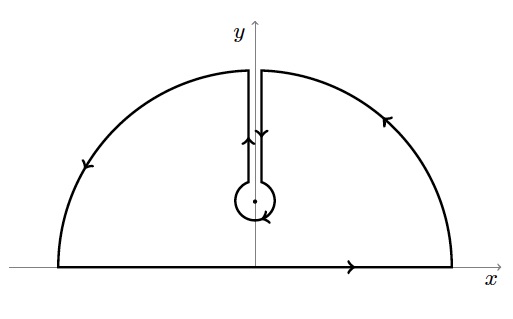
Figure 3: Integration contour.

In order to obtain configuration-space expressions for the N4LO axial current, we need the following Fourier transforms of the loop functions (with the asymptotic polynomials subtracted out as in the previous subsection)

$$F_{i}(r)=\int\frac{d{\bf k}}{(2\pi)^{3}}\,{\rm e}^{-i{\bf k}\cdot{\bf r}}\,W_{i}(k)\ ,\qquad G_{i}(r)=\int\frac{d{\bf k}}{(2\pi)^{3}}\,{\rm e}^{-i{\bf k}\cdot{\bf r}}\,Z_{i}(k)\ ,\qquad H_{i}(r)=\int\frac{d{\bf k}}{(2\pi)^{3}}\,{\rm e}^{-i{\bf k}\cdot{\bf r}}\,\frac{Z_{i}(k)}{k^{2}+m_{\pi}^{2}}\ ,$$ (57)

which can be generically expressed as

$$\int\frac{d{\bf k}}{(2\pi)^{3}}\,{\rm e}^{-i{\bf k}\cdot{\bf r}}\,f(k)=\frac{(2\,m_{\pi})^{3}}{2\,\pi^{2}}\,\frac{1}{\lambda}\int_{0}^{\infty}dx\,x\,{\rm sin}(x\lambda)\,f(x)\ ,\qquad\lambda=2\,m_{\pi}\,r\ .$$ (58)

We carry out the integrals above by utilizing contour integration in the complex plane. We illustrate the procedure by considering

$$F_{3}(\lambda)=\frac{(2\,m_{\pi})^{3}}{2\,\pi^{2}}\,\frac{1}{\lambda}\int_{0}^{\infty}dx\,x\,{\rm sin}(x\lambda)\,W_{3}(x)=-\frac{(2\,m_{\pi})^{2}}{2\,\pi^{2}}\,\frac{1}{\lambda}\,I(\lambda)\ ,$$ (59)

where

$$I(\lambda)=\int_{0}^{\infty}dx\,\,{\rm sin}(x\lambda)\,\,{\rm arcsin}\frac{x}{\sqrt{1+x^{2}}}\ .$$ (60)

While this integral can be done by more elementary methods, the contour-integration technique is useful for dealing with the more complicated transforms needed above. By making use of the identity ${\rm arccos}\,\alpha=\pi/2-{\rm arcsin}\,\alpha$, we write

$$I(\lambda)=\frac{1}{2}\int^{\infty}_{-\infty}dx\,\,{\rm sin}(x\lambda)\,\,{\rm arcsin}\frac{x}{\sqrt{1+x^{2}}}=-\frac{1}{2}\,{\rm Im}\int^{\infty}_{-\infty}dx\,\,{\rm e}^{i\,x\lambda}\,\,{\rm arccos}\frac{x}{\sqrt{1+x^{2}}}\ ,$$ (61)

and are then led to consider the function of the complex variable $\eta$

$$f(\eta)=\frac{i}{2}\,{\rm ln}\frac{\eta-i}{\eta+i}\,\,{\rm e}^{i\,\eta\lambda_{\pi}}\equiv g(\eta)\,\,{\rm e}^{i\,\eta\lambda_{\pi}}\ ,$$ (62)

where we have used the relation

$${\rm arccos}\,\eta=-i\,{\rm ln}\left(\eta+i\,\sqrt{1-\eta^{2}}\right)\ .$$ (63)

The function $f(\eta)$ has branch points at $\eta=\pm\,i$, but is otherwise analytic. The upper cut is taken from $i$ to $+i\,\infty$ (along the positive imaginary axis), while the lower one from $-i$ to $-i\,\infty$ (along the negative imaginary axis). We consider the closed contour $C$ as in Fig. 3, so that

$$\oint_{C}d\eta\,f(\eta)=0\ .$$ (64)

Before evaluating the integral above, we need to consider the value of $f(\eta)$ to the right and left of the cut running along the positive imaginary axis. To this end, we define

$$\eta-i=r_{+}\,{\rm e}^{i\,\theta_{+}}\,\,\,{\rm with}\,\,\,-\frac{3\,\pi}{2}\leq\theta_{+}\leq\frac{\pi}{2}\ ,\qquad\eta+i=r_{-}\,{\rm e}^{i\,\theta_{-}}\,\,\,{\rm with}\,\,\,-\frac{\pi}{2}\leq\theta_{-}\leq\frac{3\,\pi}{2}\ ,$$ (65)

the restrictions on $\theta_{\pm}$ ensuring that the cuts are not crossed. Therefore for a given $\eta$, we have

$$g(\eta)=\frac{i}{2}\,{\rm ln}\frac{r_{+}}{r_{-}}-\frac{\theta_{+}-\theta_{-}}{2}\ ,$$ (66)

and the difference along the upper cut (corresponding to $\eta=i\,y$ with $y>0$) is given by

$$g(\eta)|_{{\rm left\,\,\,of\,\,\,cut}}-g(\eta)|_{{\rm right\,\,\,of\,\,\,cut}}=\pi\ .$$ (67)

The big arcs of radius $R$, and the small circle of radius $r$ around the brach point $+\,i$ give vanishing contributions as, respectively, $R\rightarrow\infty$ and $r\rightarrow 0$. Therefore, on the segments left and right of the upper cut, we find

$$\int_{\rm left\,\,of\,\,cut}\!\!\!\!\!\!d\eta\,f(\eta)-\int_{\rm right\,\,of\,\,cut}\!\!\!\!\!\!d\eta\,f(\eta)=\pi\int_{i}^{\,i\,\infty}d\eta\,\,{\rm e}^{i\,\eta\lambda}=i\,\pi\,\frac{{\rm e}^{-\lambda}}{\lambda}\ ,$$ (68)

and from Eq. (64) we obtain

$$\int^{\infty}_{-\infty}dx\,\,{\rm e}^{i\,x\lambda}\,\,{\rm arccos}\frac{x}{\sqrt{1+x^{2}}}+i\,\pi\,\frac{{\rm e}^{-\lambda}}{\lambda}=0\qquad{\rm or}\qquad I(\lambda)=\frac{\pi}{2}\,\frac{{\rm e}^{-\lambda}}{\lambda}\ .$$ (69)

By employing the integration technique above (in some instances, in addition to branch points simple poles also occur), we find the following expressions:

$$\frac{1}{(2\,m_{\pi})^{4}}\,F_{1}(\lambda) = \frac{1}{16\,\pi}\bigg{[}\left(1-2\,g_{A}^{2}\right)\frac{1}{\lambda}-\left(1-5\,g_{A}^{2}\right)\left(\frac{2}{\lambda^{3}}+\frac{2}{\lambda^{2}}+\frac{1}{\lambda}-\frac{2}{\lambda^{3}}\,{\rm e}^{\lambda}\right)+g_{A}^{2}\bigg{]}\frac{{\rm e}^{-\lambda}}{\lambda}\ ,$$ (70)

$$\frac{1}{(2\,m_{\pi})^{2}}\,F_{2}(\lambda) = \frac{1}{16\,\pi}\bigg{[}\left(1-g_{A}^{2}\right)\frac{{\rm e}^{-\lambda}}{\lambda^{2}}+g_{A}^{2}\,\frac{{\rm e}^{-\lambda}}{\lambda}+\left(1+2\,g_{A}^{2}\right)\Gamma(-1,\lambda)\bigg{]}\ ,$$ (71)

$$\frac{1}{(2\,m_{\pi})^{2}}\,F_{3}(\lambda) = -\frac{1}{4\,\pi}\,\,\frac{{\rm e}^{-\lambda}}{\lambda^{2}}\ ,$$ (72)

$$\frac{1}{(2\,m_{\pi})^{4}}\,G_{1}(\lambda) = -\frac{1}{2\,\pi}\left(\frac{1}{\lambda^{2}}+\frac{1}{\lambda}+\frac{1}{4}-\frac{{\rm e}^{\lambda}}{\lambda^{2}}\right)\frac{{\rm e}^{-\lambda}}{\lambda^{2}}\ ,$$ (73)

$$\frac{1}{(2\,m_{\pi})^{4}}\,G_{3}(\lambda) = -\frac{1}{8\,\pi}\left(\frac{1}{\lambda}+1-\frac{{\rm e}^{\lambda}}{\lambda}\right)\frac{{\rm e}^{-\lambda}}{\lambda^{3}}\ ,$$ (74)

$$\frac{1}{(2\,m_{\pi})^{2}}\,H_{1}(\lambda) = \frac{1}{4\,\pi}\bigg{[}\left(1+\frac{{\rm ln}\,3}{4}\right)\frac{{\rm e}^{-\lambda/2}}{\lambda}+\frac{{\rm e}^{-\lambda}}{\lambda^{2}}-\frac{1}{4}\int_{\lambda}^{\infty}dt\,{\rm e}^{-t}\,\,\frac{1}{t^{2}-\lambda^{2}/4}\bigg{]}\ ,$$ (75)

$$\frac{1}{(2\,m_{\pi})^{4}}\,H_{2}(\lambda) = -\frac{9}{16\,\pi}\bigg{[}\frac{{\rm ln}\,3}{12}\,\,\frac{{\rm e}^{-\lambda/2}}{\lambda}-\frac{{\rm e}^{-\lambda}}{\lambda^{2}}+\frac{1}{12}\int_{\lambda}^{\infty}dt\,\,{\rm e}^{-t}\,\,\frac{1}{t^{2}-\lambda^{2}/4}+\frac{4}{3\,\lambda}\,\frac{d^{2}}{d\lambda^{2}}M(\lambda)\bigg{]}\ ,$$ (76)

$$\frac{1}{(2\,m_{\pi})^{2}}\,H_{3}(\lambda) = \frac{1}{16\,\pi}\bigg{[}\left(1+\frac{3\,{\rm ln}\,3}{4}\right)\frac{{\rm e}^{-\lambda/2}}{\lambda}+\frac{{\rm e}^{-\lambda}}{\lambda^{2}}-\frac{3}{4}\int_{\lambda}^{\infty}dt\,{\rm e}^{-t}\,\,\frac{1}{t^{2}-\lambda^{2}/4}\bigg{]}\ ,$$ (77)

where we have introduced the incomplete gamma function $\Gamma(\alpha,x)$,

$$\Gamma(\alpha,x)=\int_{x}^{\infty}dt\,t^{\alpha-1}\,{\rm e}^{-t}\ ,$$ (78)

and have defined

$$M(\lambda)=\frac{{\rm e}^{-\lambda}}{\lambda}-\frac{1}{\lambda}-\frac{{\rm ln}\,3}{4}\,{\rm e}^{-\lambda/2}+\frac{\lambda}{4}\int_{\lambda}^{\infty}dt\,{\rm e}^{-t}\,\frac{1}{t^{2}-\lambda^{2}/4}\ ,$$ (79)

which enters $H_{2}(\lambda)$. The left-over integrals and their derivatives relative to $\lambda$ can be expressed in terms of incomplete gamma functions via the identities

$$\int_{\lambda}^{\infty}dt\,{\rm e}^{-t}\,\,\frac{1}{t^{2}-\lambda^{2}/4} = \frac{{\rm e}^{-\lambda/2}}{\lambda}\,\Gamma(0,\lambda/2)-\frac{{\rm e}^{\lambda/2}}{\lambda}\,\Gamma(0,3\,\lambda/2)\ ,$$ (80)

$$\frac{d}{d\lambda}\int_{\lambda}^{\infty}dt\,{\rm e}^{-t}\,\,\frac{1}{t^{2}-\lambda^{2}/4} = -\left(1+\frac{\lambda}{2}\right)\frac{{\rm e}^{-\lambda/2}}{\lambda^{2}}\,\Gamma(0,\lambda/2)+\left(1-\frac{\lambda}{2}\right)\frac{{\rm e}^{\lambda/2}}{\lambda^{2}}\,\Gamma(0,3\,\lambda/2)\ ,$$ (81)

$$\frac{d^{2}}{d\lambda^{2}}\int_{\lambda}^{\infty}dt\,{\rm e}^{-t}\,\,\frac{1}{t^{2}-\lambda^{2}/4} = \left(2+\lambda+\frac{\lambda^{2}}{4}\right)\frac{{\rm e}^{-\lambda/2}}{\lambda^{3}}\,\Gamma(0,\lambda/2)-\left(2-\lambda+\frac{\lambda^{2}}{4}\right)\frac{{\rm e}^{\lambda/2}}{\lambda^{3}}\,\Gamma(0,3\,\lambda/2)+\frac{{\rm e}^{\lambda}}{\lambda^{2}}\ .$$ (82)

A.3 Correlation functions

From the Fourier transforms above, the correlation functions entering the N4LO axial current listed in Sec. V are obtained as

$$F^{(0)}_{1}(\lambda) = \frac{g_{A}^{3}}{64\,\pi}\,\frac{1}{f_{\pi}^{4}}\,F_{1}(\lambda)$$ (83)

$$= \frac{g_{A}^{3}}{1024\,\pi^{2}}\,\frac{(2\,m_{\pi})^{4}}{f_{\pi}^{4}}\big{[}\left(1-2\,g_{A}^{2}\right)\lambda^{2}_{\pi}-\left(1-5\,g_{A}^{2}\right)\left(2+2\,\lambda+\lambda^{2}-2\,{\rm e}^{\lambda}\right)+\,g_{A}^{2}\,\lambda^{3}\big{]}\,\,\frac{{\rm e}^{-\lambda}}{\lambda^{4}}\ ,$$

$$F^{(1)}_{2}(\lambda) = \frac{g_{A}^{3}}{64\,\pi}\,\frac{(2\,m_{\pi})^{2}}{f_{\pi}^{4}}\,\frac{1}{\lambda}\frac{d}{d\lambda}F_{2}(\lambda)$$ (84)

$$= -\frac{g_{A}^{3}}{1024\,\pi^{2}}\,\frac{(2\,m_{\pi})^{4}}{f_{\pi}^{4}}\big{[}\left(1-g_{A}^{2}\right)\left(2+\lambda\right)+g_{A}^{2}\,\left(\lambda+\lambda^{2}\right)+\left(1+2\,g_{A}^{2}\right)\,\lambda\big{]}\,\,\frac{{\rm e}^{-\lambda}}{\lambda^{4}}\ ,$$

$$F^{(2)}_{2}(\lambda) = \frac{g_{A}^{3}}{64\,\pi}\,\frac{(2\,m_{\pi})^{2}}{f_{\pi}^{4}}\,\left[\frac{d^{2}}{d\lambda^{2}}F_{2}(\lambda)-\frac{1}{\lambda}\frac{d}{d\lambda}F_{2}(\lambda)\right]$$ (85)

$$= \frac{g_{A}^{3}}{1024\,\pi^{2}}\,\frac{(2\,m_{\pi})^{4}}{f_{\pi}^{4}}\big{[}\left(1-g_{A}^{2}\right)\left(8+5\,\lambda+\lambda^{2}\right)+g_{A}^{2}\left(3\,\lambda+3\,\lambda^{2}+\lambda^{3}\right)+\,\left(1+2\,g_{A}^{2}\right)\left(3\,\lambda+\lambda^{2}\right)\big{]}\,\,\frac{{\rm e}^{-\lambda}}{\lambda^{4}}\ ,$$

$$F^{(1)}_{3}(\lambda) = -\frac{g_{A}^{5}}{64\,\pi}\,\frac{(2\,m_{\pi})^{2}}{f_{\pi}^{4}}\left[\frac{d^{2}}{d\lambda^{2}}F_{3}(\lambda)+\frac{1}{\lambda}\frac{d}{d\lambda}F_{3}(\lambda)\right]=\frac{g_{A}^{5}}{256\,\pi^{2}}\,\frac{(2\,m_{\pi})^{4}}{f_{\pi}^{4}}\left(4+3\,\lambda+\lambda^{2}\right)\frac{{\rm e}^{-\lambda}}{\lambda^{4}}\ ,$$ (86)

$$F^{(2)}_{3}(\lambda) = \frac{g_{A}^{5}}{64\,\pi}\,\frac{(2\,m_{\pi})^{2}}{f_{\pi}^{4}}\left[\frac{d^{2}}{d\lambda^{2}}F_{3}(\lambda)-\frac{1}{\lambda}\frac{d}{d\lambda}F_{3}(\lambda)\right]=-\frac{g_{A}^{5}}{256\,\pi^{2}}\,\frac{(2\,m_{\pi})^{4}}{f_{\pi}^{4}}\left(8+5\,\lambda+\lambda^{2}\right)\frac{{\rm e}^{-\lambda}}{\lambda^{4}}\ ,$$ (87)

$$G^{(0)}_{1}(\lambda) = \frac{g_{A}^{3}}{64\,\pi}\,\frac{1}{f_{\pi}^{4}}\,G_{1}(\lambda)=-\frac{g_{A}^{3}}{128\,\pi^{2}}\,\frac{(2\,m_{\pi})^{4}}{f_{\pi}^{4}}\left(1+\lambda+\frac{\lambda^{2}}{4}-{\rm e}^{\lambda}\right)\frac{{\rm e}^{-\lambda}}{\lambda^{4}}\ ,$$ (88)

$$H^{(1)}_{1}(\lambda) = \frac{g_{A}^{3}}{32\,\pi}\,\frac{(2\,m_{\pi})^{2}}{f_{\pi}^{4}}\,\frac{1}{\lambda}\frac{d}{d\lambda}H_{1}(\lambda)$$ (89)

$$= \frac{g_{A}^{3}}{128\,\pi^{2}}\,\frac{(2\,m_{\pi})^{4}}{f_{\pi}^{4}}\bigg{[}-\left(1+\frac{{\rm ln}\,3}{4}\right)\left(\lambda+\frac{\lambda^{2}}{2}\right){\rm e}^{\lambda/2}-\left(2+\lambda\right)+\frac{1}{4}\left(\lambda+\frac{\lambda^{2}}{2}\right)\widetilde{\Gamma}(0,\lambda/2)$$

$$\qquad\qquad\qquad\qquad\qquad\qquad-\frac{1}{4}\left(\lambda-\frac{\lambda^{2}}{2}\right)\widetilde{\Gamma}(0,3\,\lambda/2)\bigg{]}\,\frac{{\rm e}^{-\lambda}}{\lambda^{4}}\ ,$$

$$H^{(2)}_{1}(\lambda) = \frac{g_{A}^{3}}{32\,\pi}\,\frac{(2\,m_{\pi})^{2}}{f_{\pi}^{4}}\left[\frac{d^{2}}{d\lambda^{2}}H_{1}(\lambda)-\frac{1}{\lambda}\frac{d}{d\lambda}H_{1}(\lambda)\right]$$ (90)

$$= \frac{g_{A}^{3}}{128\,\pi^{2}}\,\frac{(2\,m_{\pi})^{4}}{f_{\pi}^{4}}\bigg{[}\left(1+\frac{{\rm ln}\,3}{4}\right)\left(3\,\lambda+\frac{3\,\lambda^{2}}{2}+\frac{\lambda^{3}}{4}\right){\rm e}^{\lambda/2}+\left(8+5\,\lambda+\frac{3\,\lambda^{2}}{4}\right)$$

$$-\frac{1}{4}\left(3\,\lambda+\frac{3\,\lambda^{2}}{2}+\frac{\lambda^{3}}{4}\right)\widetilde{\Gamma}(0,\lambda/2)+\frac{1}{4}\left(3\,\lambda-\frac{3\,\lambda^{2}}{2}+\frac{\lambda^{3}}{4}\right)\widetilde{\Gamma}(0,3\,\lambda/2)\bigg{]}\,\frac{{\rm e}^{-\lambda}}{\lambda^{4}}\ ,$$

$$H^{(1)}_{3}(\lambda) = \frac{g_{A}^{3}}{32\,\pi}\,\frac{(2\,m_{\pi})^{2}}{f_{\pi}^{4}}\,\frac{1}{\lambda}\frac{d}{d\lambda}H_{3}(\lambda)$$ (91)

$$= \frac{g_{A}^{3}}{512\,\pi^{2}}\,\frac{(2\,m_{\pi})^{4}}{f_{\pi}^{4}}\bigg{[}-\left(1+\frac{3\,{\rm ln}\,3}{4}\right)\left(\lambda+\frac{\lambda^{2}}{2}\right){\rm e}^{\lambda/2}-\left(2+\lambda\right)+\frac{3}{4}\left(\lambda+\frac{\lambda^{2}}{2}\right)\widetilde{\Gamma}(0,\lambda/2)$$

$$\qquad\qquad\qquad\qquad\qquad\qquad-\frac{3}{4}\left(\lambda-\frac{\lambda^{2}}{2}\right)\widetilde{\Gamma}(0,3\,\lambda/2)\bigg{]}\,\frac{{\rm e}^{-\lambda}}{\lambda^{4}}\ ,$$

$$H^{(2)}_{3}(\lambda) = \frac{g_{A}^{3}}{32\,\pi}\,\frac{(2\,m_{\pi})^{2}}{f_{\pi}^{4}}\left[\frac{d^{2}}{d\lambda^{2}}H_{3}(\lambda)-\frac{1}{\lambda}\frac{d}{d\lambda}H_{3}(\lambda)\right]$$ (92)

$$= \frac{g_{A}^{3}}{512\,\pi^{2}}\,\frac{(2\,m_{\pi})^{4}}{f_{\pi}^{4}}\bigg{[}\left(1+\frac{3\,{\rm ln}\,3}{4}\right)\left(3\,\lambda+\frac{3\,\lambda^{2}}{2}+\frac{\lambda^{3}}{4}\right){\rm e}^{\lambda/2}+\left(8+5\,\lambda+\frac{\lambda^{2}}{4}\right)$$

$$-\frac{3}{4}\left(3\,\lambda+\frac{3\,\lambda^{2}}{2}+\frac{\lambda^{3}}{4}\right)\widetilde{\Gamma}(0,\lambda/2)+\frac{3}{4}\left(3\,\lambda-\frac{3\,\lambda^{2}}{2}+\frac{\lambda^{3}}{4}\right)\widetilde{\Gamma}(0,3\,\lambda/2)\bigg{]}\,\frac{{\rm e}^{-\lambda}}{\lambda^{4}}\ ,$$

$$L^{(1)}_{1}(\lambda) = \frac{g^{3}_{A}}{128\,\pi}\,\frac{1}{f_{\pi}^{4}}\,\frac{d}{d\lambda}G_{1}(\lambda)=\frac{g^{3}_{A}}{256\,\pi^{2}}\,\frac{(2\,m_{\pi})^{4}}{f_{\pi}^{4}}\left(4+4\,\lambda+\frac{3\,\lambda^{2}}{2}+\frac{\lambda^{3}}{4}-4\,{\rm e}^{\lambda}\right)\frac{{\rm e}^{-\lambda}}{\lambda^{5}}\ ,$$ (93)

$$L^{(1)}_{2}(\lambda) = \frac{g^{3}_{A}}{128\,\pi}\,\frac{1}{f_{\pi}^{4}}\,\frac{d}{d\lambda}H_{2}(\lambda)$$ (94)

$$= \frac{g^{3}_{A}}{512\,\pi^{2}}\,\frac{(2\,m_{\pi})^{4}}{f_{\pi}^{4}}\bigg{[}24+24\,\lambda+9\,\lambda^{2}+\frac{3\,\lambda^{3}}{2}-24\,{\rm e}^{\lambda}$$

$$+\frac{3}{8}\,\lambda^{3}\left(1+\frac{\lambda}{2}\right)\widetilde{\Gamma}(0,\lambda/2)-\frac{3}{8}\,\lambda^{3}\left(1-\frac{\lambda}{2}\right)\widetilde{\Gamma}(0,3\,\lambda/2)\bigg{]}\,\frac{{\rm e}^{-\lambda}}{\lambda^{5}}\ ,$$

where we have defined

$$\widetilde{\Gamma}(\alpha,x)={\rm e}^{x}\int_{x}^{\infty}dt\,t^{\alpha-1}\,{\rm e}^{-t}\ ,$$ (95)

and $\widetilde{\Gamma}(\alpha,x)$ is computed numerically. The correlation functions above are regularized via

$$X^{(n)}_{i}(2\,m_{\pi}r)\longrightarrow C_{R_{\rm L}}(r)\,X^{(n)}_{i}(2\,m_{\pi}r)$$ (96)

where $X$ stands for $F,G,H$, and $L$.

A.4 Contact contributions

Asymptotic polynomials only occur in the loop functions $W_{1}(k)$, $Z_{1}(k)$, and $Z_{2}(k)/(k^{2}+m_{\pi}^{2})$ (see above), and lead to contact contributions, which we regularize with the Gaussian cutoff Piarulli:2015 ; Piarulli:2016

$$C_{R_{\rm S}}(k)={\rm e}^{-R^{2}_{\rm S}\,k^{2}/4}\ .$$ (97)

We obtain

$$F^{(0)}_{1}(z;\infty) = \frac{g_{A}^{3}}{128\,\pi^{3}}\,\frac{m^{4}_{\pi}}{f_{\pi}^{4}}\,\frac{1}{\left(m_{\pi}R_{\rm S}\right)^{3}}\left[\frac{1-9\,g_{A}^{2}}{2}\,C^{(0)}(z)+\frac{1-5\,g_{A}^{2}}{8}\,\frac{\pi}{m_{\pi}R_{\rm S}}\,C^{(1)}(z)\right]\ ,$$ (98)

$$G_{1}^{(0)}(z;\infty) = \frac{g_{A}^{3}}{128\,\pi^{3}}\,\frac{m^{4}_{\pi}}{f_{\pi}^{4}}\,\frac{1}{\left(m_{\pi}R_{\rm S}\right)^{3}}\left[2\,C^{(0)}(z)+\frac{\pi}{2\,m_{\pi}R_{\rm S}}\,C^{(1)}(z)\right]\ ,$$ (99)

$$L^{(1)}_{1}(z;\infty) = \frac{g^{3}_{A}}{512\,\pi^{3}}\,\frac{m_{\pi}^{4}}{f_{\pi}^{4}}\,\frac{1}{\left(m_{\pi}R_{\rm S}\right)^{4}}\left[2\,\frac{d}{dz}C^{(0)}(z)+\frac{\pi}{2\,m_{\pi}R_{\rm S}}\,\frac{d}{dz}C^{(1)}(z)\right]\ ,$$ (100)

$$L^{(1)}_{2}(z;\infty) = \frac{g^{3}_{A}}{512\,\pi^{3}}\,\frac{m_{\pi}^{4}}{f_{\pi}^{4}}\,\frac{1}{\left(m_{\pi}R_{\rm S}\right)^{4}}\left[6\,\frac{d}{dz}C^{(0)}(z)+\frac{3\,\pi}{2\,m_{\pi}R_{\rm S}}\,\frac{d}{dz}C^{(1)}(z)\right]\ ,$$ (101)

where

$$C^{(0)}(z) = 2\,\sqrt{\pi}\,{\rm e}^{-z^{2}}\ ,$$ (102)

$$\frac{d}{dz}C^{(0)}(z) = -4\,\sqrt{\pi}\,z\,{\rm e}^{-z^{2}}\ ,$$ (103)

$$C^{(1)}(z) = \int_{0}^{\infty}dx\,x^{3}\,j_{0}(xz)\,{\rm e}^{-x^{2}/4}\ ,$$ (104)

$$\frac{d}{dz}C^{(1)}(z) = -\int_{0}^{\infty}dx\,x^{4}\,j_{1}(xz)\,{\rm e}^{-x^{2}/4}\ ,$$ (105)

and $z=r/R_{\rm S}$.

A.5 Difference between Baroni al. and Krebs et al.

For clarity, we report below the momentum-space expressions for the difference between the two derivations, denoted as TOPT Baroni:2016 and UT Krebs:2017 (in the limit of vanishing momentum transfer),

$$\Delta\,{\bf j}^{\rm N4LO}_{5,a}({\bf k};{\rm OPE}) = -\frac{7\,g_{A}^{5}}{256\,\pi}\frac{m_{\pi}}{f_{\pi}^{4}}\left[\tau_{j,a}\,{\bf k}-({\bm{\tau}}_{i}\times{\bm{\tau}}_{j})_{a}\,{\bm{\sigma}}_{i}\times{\bf k}\right]\frac{{\bm{\sigma}}_{j}\cdot{\bf k}}{k^{2}+m_{\pi}^{2}}+(i\rightleftharpoons j)\ ,$$ (106)

$$\Delta\,{\bf j}^{\rm N4LO}_{5,a}({\bf k};{\rm TPE}) = -\frac{g_{A}^{5}}{128\,\pi\,f_{\pi}^{4}}\,\tau_{j,a}\left[\widetilde{F}(k)\,{\bm{\sigma}}_{i}+\widetilde{G}(k)\,{\bf k}\,{\bm{\sigma}}_{i}\cdot{\bf k}\right]+(i\rightleftharpoons j)\ ,$$ (107)

where ${\bf k}\equiv{\bf k}_{j}=-{\bf k}_{i}$, and the loop functions are given by

$$\widetilde{F}(k) = m_{\pi}\,\frac{6\,k^{2}+20\,m_{\pi}^{2}}{k^{2}+4\,m_{\pi}^{2}}\ ,$$ (108)

$$\widetilde{G}(k) = \frac{4\,k^{2}+16\,m_{\pi}^{2}}{2\,k^{3}}\,{\rm arctan}\!\left(\!\frac{k}{2\,m_{\pi}}\!\right)-\frac{2\,m_{\pi}}{k^{2}}\,\frac{3\,k^{2}+8\,m_{\pi}^{2}}{k^{2}+4\,m_{\pi}^{2}}\ .$$ (109)

We isolate the asymptotic constant in $\widetilde{F}(k)$ as

$$\overline{F}(k)=\widetilde{F}(k)-\widetilde{F}^{\infty}\ ,\qquad\overline{F}(k)=-\frac{4\,m_{\pi}^{3}}{k^{2}+4\,m_{\pi}^{2}}\ ,\qquad\widetilde{F}^{\infty}=6\,m_{\pi}\ .$$ (110)

The Fourier transforms read

$$\widetilde{F}(\lambda)=\int_{\bf k}{\rm e}^{-i{\bf k}\cdot{\bf r}}\,\overline{F}(k) = -\frac{(2\,m_{\pi})^{4}}{8\,\pi}\,\frac{{\rm e}^{-\lambda}}{\lambda}\ ,$$ (111)

$$\widetilde{G}(\lambda)=\int_{\bf k}{\rm e}^{-i{\bf k}\cdot{\bf r}}\,\widetilde{G}(k) = \frac{(2\,m_{\pi})^{2}}{2\,\pi}\left[{\rm e}^{-\lambda}\left(\frac{1}{\lambda^{2}}-\frac{1}{2\,\lambda}\right)-\Gamma(-1,\lambda)\right]\ ,$$ (112)

and the corresponding correlation functions are obtained as

$$\widetilde{F}^{(0)}(\lambda) = \frac{g_{A}^{5}}{128\,\pi\,f_{\pi}^{4}}\,\overline{F}(\lambda)=-\frac{g_{A}^{5}}{1024\,\pi^{2}}\frac{(2\,m_{\pi})^{4}}{f_{\pi}^{4}}\,\frac{{\rm e}^{-\lambda}}{\lambda}\ ,$$ (113)

$$\widetilde{G}^{(1)}(\lambda) = \frac{g_{A}^{5}}{128\,\pi}\,\frac{(2\,m_{\pi})^{2}}{f_{\pi}^{4}}\,\frac{1}{\lambda}\frac{d}{d\lambda}\widetilde{G}(\lambda)=-\frac{g_{A}^{5}}{256\,\pi^{2}}\frac{(2\,m_{\pi})^{4}}{f_{\pi}^{4}}\left(2-\frac{\lambda}{2}-\frac{\lambda^{2}}{2}\right)\frac{{\rm e}^{-\lambda}}{\lambda^{4}}\ ,$$ (114)

$$\widetilde{G}^{(2)}(\lambda) = \frac{g_{A}^{5}}{128\,\pi}\,\frac{(2\,m_{\pi})^{2}}{f_{\pi}^{4}}\ \left[\frac{d^{2}}{d\lambda^{2}}\widetilde{G}(\lambda)-\frac{1}{\lambda}\frac{d}{d\lambda}\widetilde{G}(\lambda)\right]=\frac{g_{A}^{5}}{256\,\pi^{2}}\frac{(2\,m_{\pi})^{4}}{f_{\pi}^{4}}\left(8+\frac{\lambda}{2}-\frac{3\,\lambda^{2}}{2}-\frac{\lambda^{3}}{2}\right)\frac{{\rm e}^{-\lambda}}{\lambda^{4}}\ .$$ (115)

We write the contact contributions from the OPE and TPE terms above as

$$\!\!\Delta\,{\bf j}^{\rm N4LO}_{5,a}({\bf k};{\rm CT})\!=\!\frac{7\,g_{A}^{5}}{512\,\pi}\,\frac{m_{\pi}}{f_{\pi}^{4}}\,({\bm{\tau}}_{i}\times{\bm{\tau}}_{j})_{a}\,{\bm{\sigma}}_{i}\times{\bm{\sigma}}_{j}-\left[\frac{g_{A}^{5}}{128\,\pi\,f_{\pi}^{4}}\,\widetilde{F}^{\infty}\,\tau_{j,a}\,{\bm{\sigma}}_{i}+(i\rightleftharpoons j)\right]\ ,$$ (116)

and define the correlation functions in Eq. (41) as

$$\widetilde{I}^{(0)}(z;\infty) = \frac{7\,g_{A}^{5}}{1024\,\pi^{3}}\,\frac{m^{4}_{\pi}}{f_{\pi}^{4}}\,\frac{1}{\left(m_{\pi}R_{\rm S}\right)^{3}}\,C^{(0)}(z)\ ,$$ (117)

$$\widetilde{F}^{(0)}(z;\infty) = \frac{3\,g_{A}^{5}}{128\,\pi^{3}}\,\frac{m^{4}_{\pi}}{f_{\pi}^{4}}\,\frac{1}{\left(m_{\pi}R_{\rm S}\right)^{3}}\,C^{(0)}(z)\ .$$ (118)

References

- (1) M. Chemtob and M. Rho, Phys. Lett. B 29, 540 (1969).
- (2) D.O. Riska and G. Brown, Phys. Lett. B 32, 662 (1970).
- (3) E. Fischbach, E. Harper, Y. Kim, A. Tubis, and W. Cheng, Phys. Lett. B 38, 8 (1972).
- (4) J. Carlson, D.O. Riska, R. Schiavilla, and R.B. Wiringa, Phys. Rev. C. 44, 619 (1991).
- (5) R. Schiavilla, V.G.J. Stoks, W. Glöckle, H. Kamada, A. Nogga, J. Carlson, R. Machleidt, V.R. Pandharipande, R.B. Wiringa, A. Kievsky, S. Rosati, and M. Viviani, Phys. Rev. C 58, 1263 (1998).
- (6) M. Gari and A. Huffman, Astrophys. J. 174, L153 (1972).
- (7) F. Dautry, M. Rho, and D.O. Riska, Nucl. Phys. A 264, 507 (1976).
- (8) M.J. Savage, P.E. Shanahan, B.C. Tiburzi, M.L. Wagman, F. Winter, S.R. Beane, E. Chang, Z. Davoudi, W. Detmold, and K. Orginos (NPLQCD Collaboration), Phys. Rev. Lett. 119, 062002 (2017).
- (9) T.-S. Park, K. Kubodera, D.-P. Min, and M. Rho, Astrophys. J. 507, 443 (1998).
- (10) T.-S. Park, L.E. Marcucci, R. Schiavilla, M. Viviani, A. Kievsky, S. Rosati, K. Kubodera, D.-P. Min, and M. Rho, Phys. Rev. C 67, 055206 (2003).
- (11) L.E. Marcucci, R. Schiavilla, and M. Viviani, Phys. Rev. Lett. 110, 192503 (2013).
- (12) A. Baroni, L. Girlanda, A. Kievsky, L.E. Marcucci, R. Schiavilla, and M. Viviani, Phys. Rev. C 94, 024003 (2016); 95, 059902 (E) (2017).
- (13) P. Klos, A. Carbone, K. Hebeler, J. Menendez, A. Schwenk, Eur. Phys. J. A 53, 168 (2017).
- (14) M. Butler and J.-W. Chen, Phys. Lett. B 520, 87 (2001).
- (15) H. De-Leon, L. Platter, and D. Gazit, arXiv:1611.10004.
- (16) M. Chemtob and M. Rho, Nucl. Phys. A 163, 1 (1971).
- (17) I.S. Towner, Phys. Rep. 155, 263 (1987).
- (18) D.O. Riska, Phys. Rep. 181, 207 (1989).
- (19) A. Gardestig and D.R. Phillips, Phys. Rev. Lett. 96, 232301 (2006).
- (20) D. Gazit, S. Quaglioni, and P. Navratil, Phys. Rev. Lett. 103, 102502 (2009).
- (21) E. Epelbaum, A. Nogga, W. Gloeckle, H. Kamada, U.-G. Meissner, and H. Witala, Phys. Rev. C 66, 064001 (2002).
- (22) M. Piarulli, L. Girlanda, R. Schiavilla, A. Kievsky, A. Lovato, L.E. Marcucci, S.C. Pieper, M. Viviani, and R.B. Wiringa, Phys. Rev. C 94, 054007 (2016).
- (23) M. Piarulli, A. Baroni, L. Girlanda, A. Kievsky, A. Lovato, E. Lusk, L.E. Marcucci, S.C. Pieper, R. Schiavilla, M. Viviani, and R.B. Wiringa, Phys. Rev. Lett. 120, 052503 (2018).
- (24) A. Baroni, L. Girlanda, S. Pastore, R. Schiavilla, and M. Viviani, Phys. Rev. C 93, 015501 (2016); 93, 049902 (E) (2016); 95, 059901 (E) (2017).
- (25) R. Schiavilla, unpublished.
- (26) A. Lovato, M. Piarulli, and R.B. Wiringa, unpublished.
- (27) H. Krebs, E. Epelbaum, and U.-G. Meissner, Ann. Phys. 378, 317 (2017).
- (28) M. Piarulli, L. Girlanda, R. Schiavilla, R. Navarro Pérez, J.E. Amaro, and E. Ruiz Arriola, Phys. Rev. C 91, 024003 (2015).
- (29) H. Krebs, E. Epelbaum, and U.-G. Meissner, Eur. Phys. J. A 32, 127 (2007).
- (30) A. Gezerlis, I. Tews, E. Epelbaum, S. Gandolfi, K. Hebeler, A. Nogga, and A. Schwenk, Phys. Rev. Lett. 111, 032501 (2013).
- (31) A. Gezerlis, I. Tews, E. Epelbaum, M. Freunek, S. Gandolfi, K. Hebeler, A. Nogga, and A. Schwenk, Phys. Rev. C 90, 054323 (2014).
- (32) J.E. Lynn, J. Carlson, E. Epelbaum, S. Gandolfi, A. Gezerlis, and A. Schwenk, Phys. Rev. Lett. 113, 192501 (2014).
- (33) J.E. Lynn, I. Tews, J. Carlson, S. Gandolfi, A. Gezerlis, K.E. Schmidt, and A. Schwenk, Phys. Rev. Lett. 116, 062501 (2016).
- (34) I. Tews, S. Gandolfi, A. Gezerlis, and A. Schwenk, Phys. Rev. C 93, 024305 (2016).
- (35) S. Gandolfi, H.W. Hammer, P. Klos, J.E. Lynn, and A. Schwenk, Phys. Rev. Lett. 118, 232501 (2017).
- (36) J.E. Lynn, I. Tews, J. Carlson, S. Gandolfi, A. Gezerlis, K.E. Schmidt, and A. Schwenk, Phys. Rev. C 96, 054007 (2017).
- (37) R.N. Pérez, J.E. Amaro, and E.R. Arriola, Phys. Rev. C 88, 024002 (2013); 88, 069902(E) (2013).
- (38) D.R. Entem, and R. Machleidt, Phys. Rev. C 68, 041001 (2003).
- (39) R. Machleidt and D.R. Entem, Phys. Rep. 503, 1 (2011).
- (40) M. Hoferichter, J. Ruiz de Elvira, B. Kubis, and U.-G. Meissner, Phys. Rev. Lett. 115, 192301 (2015).
- (41) L.E. Marcucci, A. Kievsky, S. Rosati, R. Schiavilla, and M. Viviani, Phys. Rev. Lett. 108, 052502 (2012).
- (42) K. Schoen, D.L. Jacobson, M. Arif, P.R. Huffman, T.C. Black, W.M. Snow, S.K. Lamoreaux, H. Kaiser, and S.A. Werner, Phys. Rev. C 67, 044005 (2003).
- (43) A. Nogga, A. Kievsky, H. Kamada, W. Glöckle, L.E. Marcucci, S. Rosati, and M. Viviani, Phys. Rev. C 67, 034004 (2003).
- (44) P.B. Demorest, T. Pennucci, S.M. Ransom, M.S.E. Roberts, and J.W.T. Hessels, Nature 467, 1081 (2010).
- (45) J. Antoniadis et al., Science 340, 1233232 (2013).
- (46) S. Pastore, L. Girlanda, R. Schiavilla, and M. Viviani, Phys. Rev. C 84, 024001 (2011).
- (47) S. Pastore, A. Baroni, J. Carlson, S. Gandolfi, S.C. Pieper, R. Schiavilla, and R.B. Wiringa, Phys. Rev. C 97, 022501(R) (2018).
- (48) P. Navratil, talk at the ECT* workshop “Exploring the role of electro-weak currents in atomic nuclei”, April 23-27, 2018, Trento, Italy.
- (49) G. Hagen, talk at the ECT* workshop “Exploring the role of electro-weak currents in atomic nuclei”, April 23-27, 2018, Trento, Italy.
- (50) D. Gazit, S. Vaintraub, and N. Barnea, arXiv:0901.2670.
- (51) J.L. Forest, V.R. Pandharipande, S.C. Pieper, R.B. Wiringa, R. Schiavilla, and AȦrriaga, Phys. Rev. C 54, 646 (1996).