Abstract

Gaussian processes (GPs) offer a flexible class of priors for nonparametric Bayesian regression, but popular GP posterior inference methods are typically prohibitively slow or lack desirable finite-data guarantees on quality. We develop a scalable approach to approximate GP regression, with finite-data guarantees on the accuracy of our pointwise posterior mean and variance estimates. Our main contribution is a novel objective for approximate inference in the nonparametric setting: the preconditioned Fisher (pF) divergence. We show that unlike the Kullback–Leibler divergence (used in variational inference), the pF divergence bounds the 2-Wasserstein distance, which in turn provides tight bounds on the pointwise error of mean and variance estimates. We demonstrate that, for sparse GP likelihood approximations, we can minimize the pF divergence efficiently. Our experiments show that optimizing the pF divergence has the same computational requirements as variational sparse GPs while providing comparable empirical performance—in addition to our novel finite-data quality guarantees.

1 Introduction

Gaussian processes (GPs) offer a versatile class of models for functions. In particular, GPs are able to capture complex, highly non-linear relationships in data. Unfortunately, even in the setting of GP regression with Gaussian noise, exact GP inference—that is, computing the posterior mean and covariance functions of the GP given $N$ observations—incurs a prohibitive $O(N^{3})$ running time and $O(N^{2})$ memory cost (Rasmussen and Williams, 2006). By contrast, modern, large-scale data sets require algorithms with time and memory requirements at most linear in $N$. A natural question arises: can a reliably good GP approximation be found with at most linear cost? To understand what counts as a “good” approximation, we observe that practitioners tend to report pointwise estimates and uncertainties for the GP regression curve, especially pointwise posterior means and standard deviations (Sacks et al., 1989; Kaufman and Sain, 2010; Kaufman et al., 2011; Gramacy and Lee, 2012; Rasmussen and Ghahramani, 2002; Rasmussen and Williams, 2006; Snoek et al., 2012; Osborne et al., 2012). To the best of our knowledge, it is an open problem whether non-trivial, non-asymptotic theoretical bounds exist on the quality of these estimates when running linear-time approximations to GP regression. We believe we provide the first approach that simultaneously satisfies the following desiderata: (1) linear running time and memory cost in $N$, (2) theoretical bounds on the quality of pointwise estimates of the posterior mean, standard deviation, and variance for finite data, and (3) a practical mechanism for provably decreasing these bounds to zero.

Previous approaches to scaling GP inference primarily fall into two categories: sparse GP methods (Smola and Bartlett, 2000; Seeger et al., 2003; Quiñonero-Candela and Rasmussen, 2005; Snelson and Ghahramani, 2005; Titsias, 2009; Bauer et al., 2016; Hensman et al., 2013; de G Matthews et al., 2016; Bui et al., 2017) and structured kernel matrix approximations (Wilson and Nickisch, 2015; Ding et al., 2017; Katzfuss, 2017; Gardner et al., 2018; Izmailov et al., 2018). The sparse GP approach introduces a set of $M$ inducing points, which are chosen either greedily or at random and can then be optimized. The most widely used and top-performing sparse GP methods are variational and originate with the work of Titsias (2009). These methods optimize the inducing point locations using a variational evidence lower bound (Titsias, 2009; Bauer et al., 2016; Hensman et al., 2013; de G Matthews et al., 2016; Bui et al., 2017) and have $O(M^{2}N)$ time and $O(MN)$ space complexity. Structured kernel approximations replace the $N\times N$ kernel matrix with an approximation that can be represented more compactly and operated on more efficiently. The time and space requirements of these methods vary and usually depend on the dimensionality of the input space. Neither approach is guaranteed to provide accurate estimates of the posterior mean or variance. Typically, these methods are validated empirically on small datasets (Bauer et al., 2016).

In fact, after introducing GP regression in more detail in Section 2, we note in Section 3 that a posterior approximation can be close in Kullback-Leibler (KL) divergence to the exact posterior and still exhibit bad posterior mean and variance approximations. Thus, rather than pursue variational methods with KL divergence, we instead observe that closeness in 2-Wasserstein distance implies closeness of means and covariances—as well as many other posterior functionals (e.g. expectations of any function with a bounded gradient). For GPs, it is not possible to efficiently compute the 2-Wasserstein distance to the exact posterior, so instead we develop a theoretically-motivated proxy.

In particular, we build from a related metric called the Fisher distance. The squared Fisher distance between two distributions is defined as the expected squared norm of the difference between their score functions. This distance has been successfully applied in the finite-dimensional setting both to design practical algorithms (Campbell and Broderick, 2019) and for theoretical analysis (Huggins and Zou, 2017; Ogden, 2017). In Section 4, we adapt the Fisher distance to the infinite-dimensional GP setting and call our new measure of fit the preconditioned Fisher (pF) divergence. We carefully design the pF divergence to work with likelihoods that are parameterized by functions—as opposed to, e.g., the finite vector parameters that are more familiar from the parametric setting. We show that the pointwise mean and variance approximation errors are bounded by a constant times the pF divergence, and thus minimizing the pF divergence results in small mean and variance approximation error. In Section 5 we demonstrate that the pF divergence can be computed and efficiently minimized for a sparse GP likelihood approximation. Our experiments in Section 6 on simulated and real data show that our method (1) yields comparable empirical performance with the existing state-of-the-art variational methods while (2) using as much or less computation. Thus, using the pF divergence as an objective for approximate GP inference is a promising alternative to the variational approach, offering state-of-the-art real-world performance while crucially providing finite-data guarantees on the accuracy of the posterior mean and variance estimates.

2 Sparse Gaussian process regression

A Gaussian process on covariate space $\mathcal{X}$ is determined by a mean function ${\mu:\mathcal{X}\to\mathbb{R}}$ and a positive-definite covariance, or kernel, function ${k:\mathcal{X}\times\mathcal{X}\to\mathbb{R}}$. Take any two sets of locations $\bm{X}=(\bm{x}_{1},\dots,\bm{x}_{N})\in\mathcal{X}^{N}$ and $\bm{X}^{\prime}=(\bm{x}_{1}^{\prime},\dots,\bm{x}_{N^{\prime}}^{\prime})\in\mathcal{X}^{N^{\prime}}$ and any function $f:\mathcal{X}\to\mathbb{R}$. Let $f_{\bm{X}}:=(f(\bm{x}_{1}),\dots,f(\bm{x}_{N}))$, and let $k_{\bm{X}\bm{X}^{\prime}}$ be the $N\times N^{\prime}$ matrix where $[k_{\bm{X}\bm{X}^{\prime}}]_{nn^{\prime}}=k(\bm{x}_{n},\bm{x}_{n^{\prime}}^{\prime})$. If $f\sim{\mathrm{GP}}(\mu,k)$ is a GP-distributed function, $f$ is marginally Gaussian at any set of locations: $f_{\bm{X}}\sim\mathcal{N}(\mu_{\bm{X}},k_{\bm{X}\bm{X}})$.

In GP regression (Rasmussen and Williams, 2006), we model noisy observed output $y_{n}$ at input location $\bm{x}_{n}$:

$$y_{n}\,|\,f,\bm{x}_{n} \overset{\textrm{{indep}}}{\sim}\mathcal{N}(f(\bm{x}_{n}),\sigma^{2}),\quad n=1,\dots,N$$

$$f \sim{\mathrm{GP}}(0,k),$$

where $\sigma^{2}>0$ is the observation noise variance and we make a standard assumption that the mean function is identically zero. We collect the response variables as $\bm{y}:=(y_{1}\dots,y_{N})\in\mathbb{R}^{N}$. The posterior distribution given the data ${\bm{D}}=(\bm{X},\bm{y})$ is the Gaussian process $\pi={\mathrm{GP}}(\mu_{{\bm{D}}},k_{{\bm{D}}})$, where $\mu_{{\bm{D}}}(\bm{x}):=k_{\bm{x}\bm{X}}[k_{\bm{X}\bm{X}}+\sigma^{2}I]^{-1}\bm{y}$ and $k_{{\bm{D}}}(\bm{x},\bm{x}^{\prime}):=k(\bm{x},\bm{x}^{\prime})-k_{\bm{x}\bm{X}}[k_{\bm{X}\bm{X}}+\sigma^{2}I]^{-1}k_{\bm{X}\bm{x}^{\prime}}$ are, respectively, the posterior mean and kernel functions. The posterior mean and kernel functions are usually the quantities of interest since they fully define the GP posterior distribution. They can then be used for prediction, in Bayesian optimization, in the design of computer experiments, and for other tasks (Sacks et al., 1989; Kaufman and Sain, 2010; Kaufman et al., 2011; Gramacy and Lee, 2012; Rasmussen and Ghahramani, 2002; Rasmussen and Williams, 2006; Snoek et al., 2012; Osborne et al., 2012). Computing the posterior exactly requires $O(N^{3})$ time due to the cost of inversion of the $N\times N$ matrix $k_{\bm{X}\bm{X}}+\sigma^{2}I$. Sparse Gaussian process approximations make GP inference more scalable by introducing a set of $M$ inducing points $\bm{\tilde{X}}=(\bm{\tilde{x}}_{1},\dots,\bm{\tilde{x}}_{m})$ and evaluating the function $f$ only at those locations (Seeger et al., 2003; Quiñonero-Candela and Rasmussen, 2005; Snelson and Ghahramani, 2005; Titsias, 2009). The key idea is to replace the exact log-likelihood $\mathcal{L}(f):=\log p_{\mathcal{N}}(\bm{y}\,|\,f_{\bm{X}},\sigma^{2}I)$ with an approximate log-likelihood that makes use of the observation that if $f\sim{\mathrm{GP}}(0,k)$, then $\mathbb{E}[f_{\bm{X}}\,|\,f_{\bm{\tilde{X}}}]=k_{\bm{X}\bm{\tilde{X}}}k_{\bm{\tilde{X}}\bm{\tilde{X}}}^{-1}f_{\bm{\tilde{X}}}$. For example, the deterministic training conditional (DTC) approximation (Seeger et al., 2003; Quiñonero-Candela and Rasmussen, 2005) is $\tilde{\mathcal{L}}_{\text{DTC}}(f):=\log p_{\mathcal{N}}(\bm{y}\,|\,k_{\bm{X}\bm{\tilde{X}}}k_{\bm{\tilde{X}}\bm{\tilde{X}}}^{-1}f_{\bm{\tilde{X}}},\sigma^{2}I)$.

3 Wasserstein and Fisher distances

Scalable GP inference methods based on optimizing a variational lower bound for the model evidence have so far provided the best empirical performance when compared to alternative methods (Titsias, 2009; Bauer et al., 2016; Hensman et al., 2013, 2015). While variational inference is an elegant approach, there are no finite-data guarantees on the accuracy of the approximate mean and covariance functions produced by variational methods. The issue is that variational methods minimize the KL divergence between the sparse posterior approximation and the exact posterior (Titsias, 2009; Bauer et al., 2016; Hensman et al., 2013), but a small KL divergence does not necessarily imply small error in the mean and covariance estimates. For clarity, we consider the case of finite-dimensional Gaussians.

Proposition 3.1.

$\forall\delta>0$ there exist distributions $\eta=\mathcal{N}(\mu,s^{2})$ and $\tilde{\eta}=\mathcal{N}(\tilde{\mu},\tilde{s}^{2})$ on $\mathbb{R}$ such that $\mathrm{KL}(\tilde{\eta}||\eta)=\delta$, $(\mu-\tilde{\mu})^{2}=\tilde{s}^{2}\{\exp(2\delta)-1\}$, and $\tilde{s}^{2}=\exp(-2\delta)s^{2}$.

See proof in Appendix B. Proposition 3.1 shows that, for example, if $\mathrm{KL}(\tilde{\eta}||\eta)=5$ then the mean estimate may be off by more than $148\tilde{s}$. Since $\tilde{s}$ provides a natural unit of uncertainty about the parameter value, we see that a moderate Kullback–Leibler divergence can correspond to a very large error in the mean estimate.

An alternative to KL divergences that does imply closeness of means and covariances is the 2-Wasserstein distance. For the remainder of the paper let $\eta$, $\tilde{\eta}$, and $\nu$ denote probability measures on a measurable space $(\mathbb{H},\mathcal{B})$, where $(\mathbb{H},\langle{\cdot},{\cdot}\rangle_{\mathbb{H}})$ is a Hilbert space. We assume these distributions are absolutely continuous with respect to a base measure $\lambda$. We will typically take $\eta$ to be the GP regression posterior $\pi$, $\tilde{\eta}$ to be an approximation $\tilde{\pi}$ to the posterior, and $\lambda$ to be the prior $\pi_{0}$. Let $\Gamma(\eta,\tilde{\eta})$ denote the collection of distributions $\gamma$ on $\mathbb{H}\times\mathbb{H}$ such that $\gamma$ has marginal distributions $\eta$ and $\tilde{\eta}$: that is, $\eta=\gamma(\cdot,\mathbb{H})$ and $\tilde{\eta}=\gamma(\mathbb{H},\cdot)$. The $2$-Wasserstein distance between $\eta$ and $\tilde{\eta}$ is given by

$$\mathcal{W}_{2}(\eta,\tilde{\eta}):=\inf_{\gamma\in\Gamma(\eta,\tilde{\eta})}\bigg{\{}\int\|{\theta-\tilde{\theta}}\|_{\mathbb{H}}^{2}\gamma(\mathrm{d}\theta,\mathrm{d}\tilde{\theta})\bigg{\}}^{1/2}.$$

Closeness in 2-Wasserstein implies closeness of means, standard deviations, and many other expectations:

Proposition 3.2.

Assume that $\mathbb{H}=\mathbb{R}$, that $\eta$ has mean $\mu$ and variance $s^{2}$, and that $\tilde{\eta}$ has mean $\tilde{\mu}$ and variance $\tilde{s}^{2}$. If $\mathcal{W}_{2}(\eta,\tilde{\eta})\leq\varepsilon$, then $|\mu-\tilde{\mu}|\leq\varepsilon$, $|s-\tilde{s}|\leq 2\varepsilon$, and, for any function $\phi:\mathbb{R}\to\mathbb{R}$ such that $|\mathrm{d}\phi/\mathrm{d}\theta|\leq L<\infty$, $|\mathbb{E}_{\theta\sim\eta}[\phi(\theta)]-\mathbb{E}_{\tilde{\theta}\sim v}[\phi(\tilde{\theta})]\leq L\epsilon$.

Similar results hold for distributions in $\mathbb{R}^{d}$ and for Gaussian processes (detailed later in Theorems 4.3 and D). Unfortunately it is not feasible to directly minimize the 2-Wasserstein distance between the exact posterior $\pi$ and some approximation $\tilde{\pi}$ because it would require computing the posterior, including its normalizing constant. Therefore, we introduce an alternative divergence measure we call the $\nu$-Fisher distance. Crucially, the $\nu$-Fisher distance satisfies two properties: (1) it does not depend on the normalizing constant of the target distribution, so it can be computed in practice, and (2) it provides an upper bound on the 2-Wasserstein distance, so it provides accuracy guarantees on means and standard deviations. Let $L^{2}(\nu)$ denote the space of functions that are square-integrable with respect to $\nu$: $\phi\in L^{2}(\nu)\implies\left\|{\phi}\right\|_{L^{2}(\nu)}:=(\int\phi(\theta)^{2}\nu(\mathrm{d}\theta))^{1/2}<\infty$.

Definition 3.3.

When $\mathbb{H}=\mathbb{R}^{d}$, the $\nu$-Fisher distance between two distributions is defined as the square root of the expected squared Euclidean distance between the score functions of the two densities:

$$d_{\mathrm{F},\nu}(\eta,\tilde{\eta}):=\left\|{\Big{\|}\nabla\log\frac{\mathrm{d}\tilde{\eta}}{\mathrm{d}\theta}-\nabla\log\frac{\mathrm{d}\eta}{\mathrm{d}\theta}\Big{\|}_{2}}\right\|_{L^{2}(\nu)}$$

The $\nu$-Fisher distance implies the following 2-Wasserstein bound, which for simplicity we state for the most relevant case of when $\eta$ and $\tilde{\eta}$ are (finite-dimensional) Gaussians. For a matrix $A$, let $\sigma_{\mathrm{min}}(A)$ denote the smallest absolute eigenvalue of $A$ and for a function $\phi$, let $\left\|{\phi}\right\|_{\infty}$ denote the usual sup-norm.

Proposition 3.4.

Assume $\mathbb{H}=\mathbb{R}^{d}$, $\eta=\mathcal{N}(\mu,\Sigma)$, $\tilde{\eta}=\mathcal{N}(\tilde{\mu},\tilde{\Sigma})$. Then for any probability measure $\nu$ such that $\eta\ll\nu$, $\mathcal{W}_{2}(\eta,\tilde{\eta})\leq\sigma_{\mathrm{min}}(\tilde{\Sigma})^{-1}\left\|{\mathrm{d}\eta/\mathrm{d}\nu}\right\|_{\infty}^{1/2}d_{\mathrm{F},\nu}(\eta,\tilde{\eta}).$

The special case when $\nu=\eta$ or $\tilde{\eta}$ is known as (e.g.) the Fisher divergence and has appeared in many applications. It serves as the objective in score matching, a model estimation technique (Sriperumbudur et al., 2017; Hyvarinen, 2005). Johnson and Barron (2004) and Ley and Swan (2013) bounded certain integral probability measures (e.g. the total variation and Kolmogorov distances) in terms of the Fisher divergence while Huggins and Zou (2017) bounded the 1-Wasserstein distance in terms of the Fisher divergence. In the Bayesian setting, Campbell and Broderick (2019, 2018) minimized the $\nu$-Fisher distance to construct a high-quality posterior approximation based on a coreset. Campbell and Broderick (2019, 2018) found their coreset method performed very well empirically, including accurate posterior mean and variance estimates. Ogden (2017) and Dalalyan and Karagulyan (2017) developed related guarantees—the former using a score function approach similar in spirit to the $\nu$-Fisher distance. Finally, Huggins et al. (2017) used the results of Huggins and Zou (2017) to prove finite-data Wasserstein guarantees for a scalable approximate inference algorithm for generalized linear models.

4 Infinite-dimensional spaces

Together, Propositions 3.2 and 3.4 show that small $\nu$-Fisher distance between two finite-dimensional Gaussians implies small differences in their means and standard deviations. Based on these theoretical foundations and the empirical successes of Campbell and Broderick (2019, 2018), the $\nu$-Fisher distance appears to be an attractive objective for optimizing the sparse GP likelihood approximation. However, there are a number of subtleties that must be addressed before using this distance, or a similar distance, for GP regression—in particular, due to the infinite-dimensional parameter space in this case. In the GP setting the Hilbert space $\mathbb{H}$ is a function space, so instead of gradients of the log-likelihood, we must use a functional derivative $\mathcal{D}$, taken with respect to the Hilbert norm $\left\|{\cdot}\right\|_{\mathbb{H}}$. That is, for a function $F:\mathbb{H}\to\mathbb{R}$, $\mathcal{D}F:\mathbb{H}\to\mathbb{H}$ is the linear operator that satisfies $\lim_{h\to 0}\left\|{F(f+h)-F(f)-(\mathcal{D}F)(h)}\right\|_{\mathbb{H}}/\left\|{h}\right\|_{\mathbb{H}}=0$ for all $f\in\mathbb{H}$. The major obstacle to overcome is that the naïve extension of the $\nu$-Fisher distance can differ from the 2-Wasserstein distance by an arbitrarily large multiplicative factor. If we tried to directly translate the $\nu$-Fisher distance to the GP setting we would get

$$d_{\mathrm{F},\nu}(\eta,\tilde{\eta}):=\left\|{\Big{\|}\mathcal{D}\log\frac{\mathrm{d}\tilde{\eta}}{\mathrm{d}\lambda}-\mathcal{D}\log\frac{\mathrm{d}\eta}{\mathrm{d}\lambda}\Big{\|}_{\mathbb{H}}}\right\|_{L^{2}(\nu)}.$$

Notice that the derivatives are now functional derivatives and that the Radon-Nikodym derivatives are no longer with respect to Lebesgue measure, but rather with respect to the base measure $\lambda$.

To gain intuition for what can go wrong in the infinite-dimensional setting, recall from Proposition 3.4 that in the finite-dimensional Gaussian case, the constant in the bound depends on $\sigma_{\mathrm{min}}(\tilde{\Sigma})^{-1}$, the reciprocal of smallest eigenvalue of the covariance of $\tilde{\eta}$. In infinite dimensions, we replace $\tilde{\Sigma}$ with the covariance operator $\mathcal{C}_{\tilde{\eta}}$ associated with $\tilde{\eta}$ (Ibragimov and Rozanov, 1978, Ch. 1.4), the formal definition of which we defer. The eigenvalues of $\mathcal{C}_{\tilde{\eta}}$ get arbitrarily close to zero, so $\sigma_{\mathrm{min}}(\mathcal{C}_{\tilde{\eta}})^{-1}=\infty$ and the bound is vacuous. The next example illustrates the issue for GP regression.

Example 4.1.

Consider a 1-dimensional Gaussian process on $\mathcal{X}=\mathbb{R}$ with squared exponential kernel $k(x,x^{\prime})=e^{-(x-x^{\prime})^{2}/2}$. Let $\eta$ (respectively $\tilde{\eta}$) denote the GP regression posterior distribution with $N=1$, $x_{1}=0$, and $y_{1}=t$ (resp. $y_{1}=\tilde{t}\,$). Then $d_{\mathrm{F},\nu}(\eta,\tilde{\eta})=c(1+\sigma^{-2})\mathcal{W}_{2}(\eta,\tilde{\eta})$, where $c$ is a constant that depends on the choice of $\mathbb{H}$ and the factor of $(1+\sigma^{-2})$ can be made arbitrarily large by taking $\sigma^{2}\to 0$. See Appendix C for a detailed derivation.

4.1 shows that the Fisher divergence bound on the Wasserstein distance could be arbitrarily large even when the Wasserstein distance itself is finite. To understand how to fix the problem, we can take inspiration from the finite-dimensional setting; suppose $\tilde{\Sigma}$ had a very small but non-zero eigenvalue. We could perform a change of basis: $\theta\mapsto\tilde{\Sigma}^{1/2}\theta$. In the new basis, $\tilde{\eta}$ would have covariance equal to the identity matrix $I$, and hence the minimum eigenvalue would be one. Working with the score function, this change of variable corresponds to replacing $\nabla\log\frac{\mathrm{d}\tilde{\eta}}{\mathrm{d}\theta}(\theta)=-\tilde{\Sigma}^{-1}(\theta-\tilde{\mu})$ with $\tilde{\Sigma}\nabla\log\pi(\theta)=-(\theta-\tilde{\mu})$, where the final expression is equal to the gradient of the log density of a Gaussian with covariance $I$. Formally, this procedure carries over to the infinite-dimensional case: we replace the functional derivative $\mathcal{D}$ with $\mathcal{C}_{\tilde{\eta}}\mathcal{D}$.

To precisely define the covariance operator, we must describe the Hilbert space $\mathbb{H}$ in more detail. Specifically, we will take $\mathbb{H}$ to be a reproducing kernel Hilbert space (RKHS) (Steinwart and Christmann, 2008, Ch. 4). For a positive definite reproducing kernel $r:\mathcal{X}\times\mathcal{X}\to\mathbb{R}$, the corresponding RKHS $\mathbb{H}_{r}$ comes equipped with an inner product $\langle{\cdot},{\cdot}\rangle_{r}$. The function $r_{\bm{x}}:=r(\bm{x},\cdot)$ is the evaluation function at $\bm{x}$ (that is, the inner product and reproducing kernel satisfy the reproducing property): for any $f\in\mathbb{H}_{r}$ and $\bm{x}\in\mathcal{X}$, $\langle{r_{\bm{x}}},{f}\rangle_{r}=f(\bm{x})$. We take $r$ to be fixed but for clarity make the $r$-dependence explicit. Now we can define the covariance operator $\mathcal{C}_{\tilde{\eta}}$ associated with a distribution $\tilde{\eta}$ as the self-adjoint operator that satisfies the identity $\langle{r_{\bm{x}}},{\mathcal{C}_{\tilde{\eta}}r_{\bm{x}^{\prime}}}\rangle_{r}=\operatorname{Cov}(f(\bm{x}),f(\bm{x}^{\prime}))$, where $f\sim\tilde{\eta}$.

Remark 4.1.

We emphasize the very different roles played by the kernels $k$ and $r$. Whereas $k$ determines the prior covariance of the Gaussian process used for regression, $r$ induces a reproducing kernel Hilbert space $\mathbb{H}_{r}$. Recall that $\eta$ and $\tilde{\eta}$ should be thought of as exact and approximating GP regression posterior distributions, which depend on the choice of $k$. On the other hand, for a sample $f\sim\eta$ or $\tilde{\eta}$, by construction $f\in\mathbb{H}_{r}$. But, as we discuss further below, $f\notin\mathbb{H}_{k}$ almost surely.

We can give our definition of the modified $\nu$-Fisher distance, which we call the $\nu$-preconditioned Fisher ($\nu$-pF) divergence.

Definition 4.2.

The $\nu$-preconditioned Fisher divergence is defined by

$$d_{\mathrm{pF},\nu}(\tilde{\eta}||\eta):=\left\|{\Big{\|}\mathcal{C}_{\tilde{\eta}}\mathcal{D}\log\frac{\mathrm{d}\tilde{\eta}}{\mathrm{d}\lambda}-\mathcal{C}_{\tilde{\eta}}\mathcal{D}\log\frac{\mathrm{d}\eta}{\mathrm{d}\lambda}\Big{\|}_{r}}\right\|_{L^{2}(\nu)}.$$

In the setting of 4.1, we can show that $d_{\mathrm{pF},\nu}(\tilde{\eta}||\eta)=\mathcal{W}_{2}(\eta,\tilde{\eta})$ (see Appendix C). For a distribution $\eta$, let $\mu_{\eta}(\bm{x}):=\mathbb{E}_{f\sim\eta}[f(\bm{x})]$ and $k_{\eta}(\bm{x},\bm{x}^{\prime}):=\mathbb{E}_{f\sim\eta}[(f(\bm{x})-\mu_{\eta}(\bm{x}))(f(\bm{x}^{\prime})-\mu_{\eta}(\bm{x}^{\prime}))]$ denote the mean and covariance functions associated with $\eta$. More generally, we have the following powerful result:

Theorem 4.3.

Let $\eta$, $\tilde{\eta}$, and $\nu$ denote probability measures on the measurable space $(\mathbb{H}_{r},\mathcal{B})$, all absolutely continuous with respect to a base measure $\lambda$. Assume $\eta$, $\tilde{\eta}$, and $\lambda$ are Gaussian measures. Let $\varepsilon:=\left\|{\mathrm{d}\eta/\mathrm{d}\nu}\right\|_{\infty}^{1/2}d_{\mathrm{pF},\nu}(\tilde{\eta}||\eta)$ and $\underline{k}(\bm{x},\bm{x}):=k_{\tilde{\eta}}(\bm{x},\bm{x})\wedge k_{\eta}(\bm{x},\bm{x})$. If $\varepsilon<\infty$, then $\mathcal{W}_{2}(\eta,\tilde{\eta})\leq\varepsilon$ and $\forall\bm{x}\in\mathcal{X}$,

$$|\mu_{\tilde{\eta}}(\bm{x})-\mu_{\eta}(\bm{x})| \leq r(\bm{x},\bm{x})^{1/2}\varepsilon$$

$$|k_{\tilde{\eta}}(\bm{x},\bm{x})^{1/2}-k_{\eta}(\bm{x},\bm{x})^{1/2}| \leq\mathchoice{{\hbox{$\displaystyle\sqrt{6\,}$}\lower 0.4pt\hbox{\vrule height=6.44444pt,depth=-5.15558pt}}}{{\hbox{$\textstyle\sqrt{6\,}$}\lower 0.4pt\hbox{\vrule height=6.44444pt,depth=-5.15558pt}}}{{\hbox{$\scriptstyle\sqrt{6\,}$}\lower 0.4pt\hbox{\vrule height=4.51111pt,depth=-3.6089pt}}}{{\hbox{$\scriptscriptstyle\sqrt{6\,}$}\lower 0.4pt\hbox{\vrule height=3.22221pt,depth=-2.57779pt}}}r(\bm{x},\bm{x})^{1/2}\varepsilon$$

$$|k_{\tilde{\eta}}(\bm{x},\bm{x})-k_{\eta}(\bm{x},\bm{x})| \leq 3\,r(\bm{x},\bm{x})^{1/2}\underline{k}(\bm{x},\bm{x})^{1/2}\varepsilon$$

$$\phantom{\leq\ }+6\,r(\bm{x},\bm{x})\varepsilon^{2},$$

and, for any $\phi:\mathbb{H}\to\mathbb{R}$ such that $|\mathcal{D}\phi|\leq L<\infty$,

$$|\mathbb{E}_{\tilde{f}\sim\tilde{\eta}}[\phi(\tilde{f})]-\mathbb{E}_{f\sim\eta}[\phi(f)]|\leq L\epsilon.$$

The proof of Theorem 4.3 (found in Appendix D) does not require $\eta$ and $\tilde{\eta}$ to be Gaussian measures, but for simplicity we have stated it for that case. As long as $\nu$ is an over-approximation of $\eta$ then we can use the $\nu$-pF divergence to control the 2-Wasserstein distance. By “over-approximation” we mean that $\nu$ has heavier tails than $\eta$ so $\left\|{\mathrm{d}\eta/\mathrm{d}\nu}\right\|_{\infty}$ is bounded. A bound on the 2-Wasserstein distance between $\eta$ and $\tilde{\eta}$ implies control on the difference in their mean and covariance functions. The factors of $r(\bm{x},\bm{x})^{1/2}$ account for the structure of the functions sampled from the GP.

In our application of Theorem 4.3 we will take $\eta=\pi$, the exact posterior; $\tilde{\eta}=\tilde{\pi}$, the approximate posterior; and $\lambda=\pi_{0}$, the prior. Therefore $\log\frac{\mathrm{d}\pi}{\mathrm{d}\pi_{0}}(f)=\mathcal{L}(f)$, the exact log-likelihood, and $\log\frac{\mathrm{d}\tilde{\pi}}{\mathrm{d}\pi_{0}}(f)=\tilde{\mathcal{L}}(f)$, the approximate log-likelihood. In order to make use of the pF divergence algorithmically, we must choose three free parameters: (1) the reproducing kernel $r$, (2) the auxiliary distribution $\nu$, and (3) a family of log-likelihood approximations $\tilde{\mathcal{L}}$. We address these choices in Section 4.1, Section 4.2, and Section 5, respectively.

Remark 4.4.

A direct computation of the constant $\varepsilon$ in Theorem 4.3 is difficult in practice. However, it could be approximated by taking $\nu=\eta$ and using an importance sampling approach to estimate $d_{\mathrm{pF},\eta}(\tilde{\eta}||\eta)$.

4.1 Choosing the reproducing kernel

The seemingly natural choice for the reproducing kernel $r$ is $k$. However, $\mathbb{H}_{k}$ is not suitable because if $\mathbb{H}_{k}$ is infinite-dimensional (as is almost always the case in practice), then for $f\sim{\mathrm{GP}}(0,k)$, $\mathbb{P}\{f\in\mathbb{H}_{k}\}=0$ (see Lukic and Beder (2001) and Rasmussen and Williams (2006, Ch. 6.1)). Therefore we must choose some $r\neq k$ for which $\mathbb{P}\{f\in\mathbb{H}_{r}\}=1$. The following result (proved in Appendix E) greatly simplifies the issue:

Proposition 4.5.

Suppose $\mathbb{H}_{k}$ has an orthonormal basis $(e_{j})_{j\geq 1}$ such that for any $\bm{x}\in\mathcal{X}$, $\left|e_{j}(\bm{x})\right|=o(j^{-1})$ as $j\to\infty$. Then for any finite set of points ${\bm{S}}$ and $\epsilon>0$, there exists a kernel $r$ that satisfies $\mathbb{P}\{f\in\mathbb{H}_{r}\}=1$ and $\max_{\bm{x},\bm{x}^{\prime}\in{\bm{S}}}|k(\bm{x},\bm{x}^{\prime})-r(\bm{x},\bm{x}^{\prime})|<\epsilon$.

The decay condition $\left|e_{j}(\bm{x})\right|=o(j^{-1})$ is satisfied for Gaussian kernels (Steinwart and Christmann, 2008) and we suspect for Matérn kernels as well. Since we can take $\epsilon$ arbitrarily small (e.g. smaller than floating point error), as a practical matter we can choose $r=k$. Furthermore, since in the GP regression setting we only need to evaluate the posterior approximation at a finite number of locations (say, the training points $\bm{X}$ and some additional test locations $\bm{X}^{*}$), the restriction that ${\bm{S}}$ be a finite set is not problematic. Hence, we use $r=k$ in our experiments. In the kernel regression literature, our current approach is most closely related to fixed-design error bounds (Cortes et al., 2010; El Alaoui and Mahoney, 2015); but choosing $r\neq k$ might allow more powerful generalization guarantees (Caponnetto and De Vito, 2007; Rudi et al., 2015).

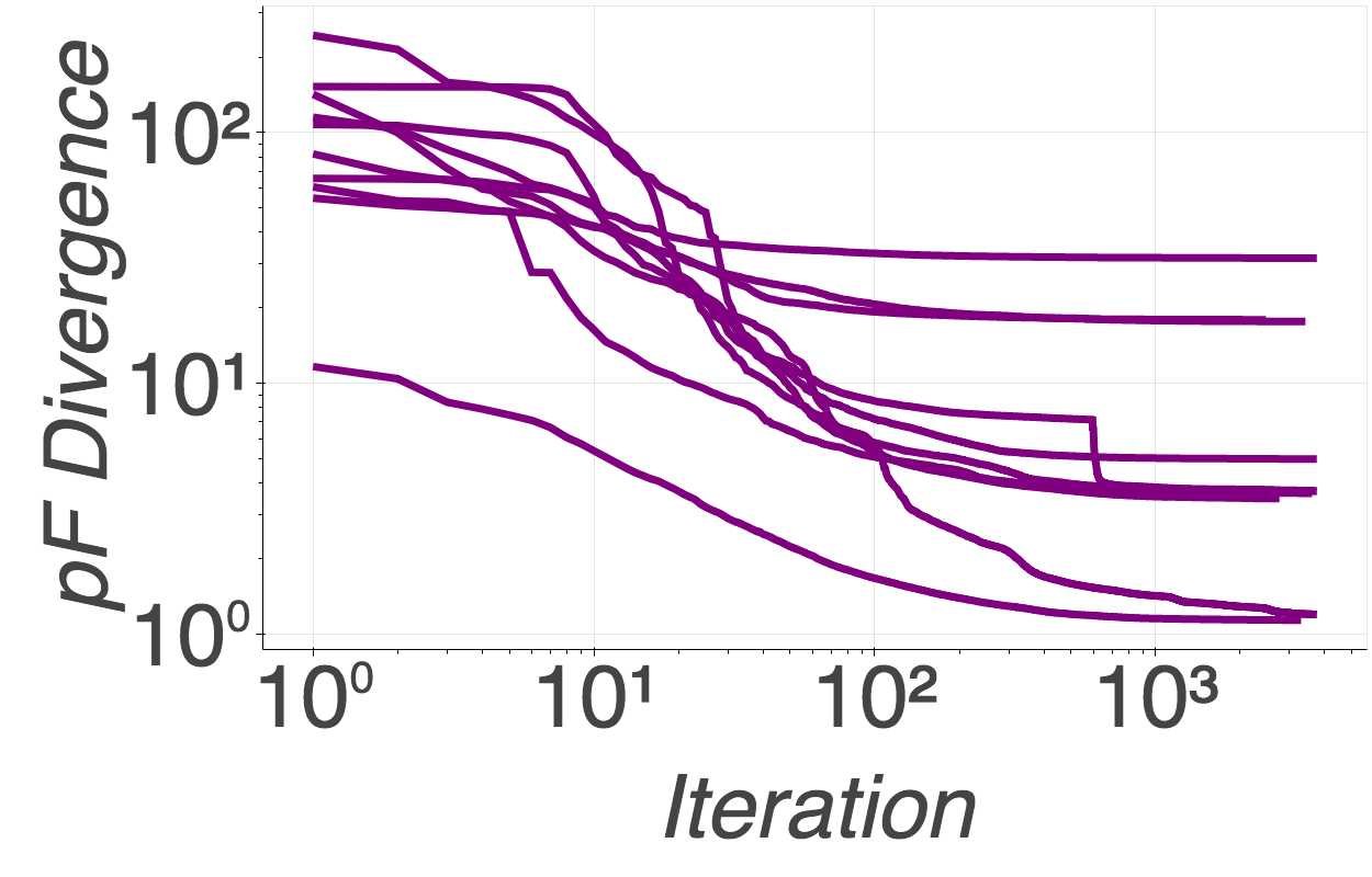
(a)

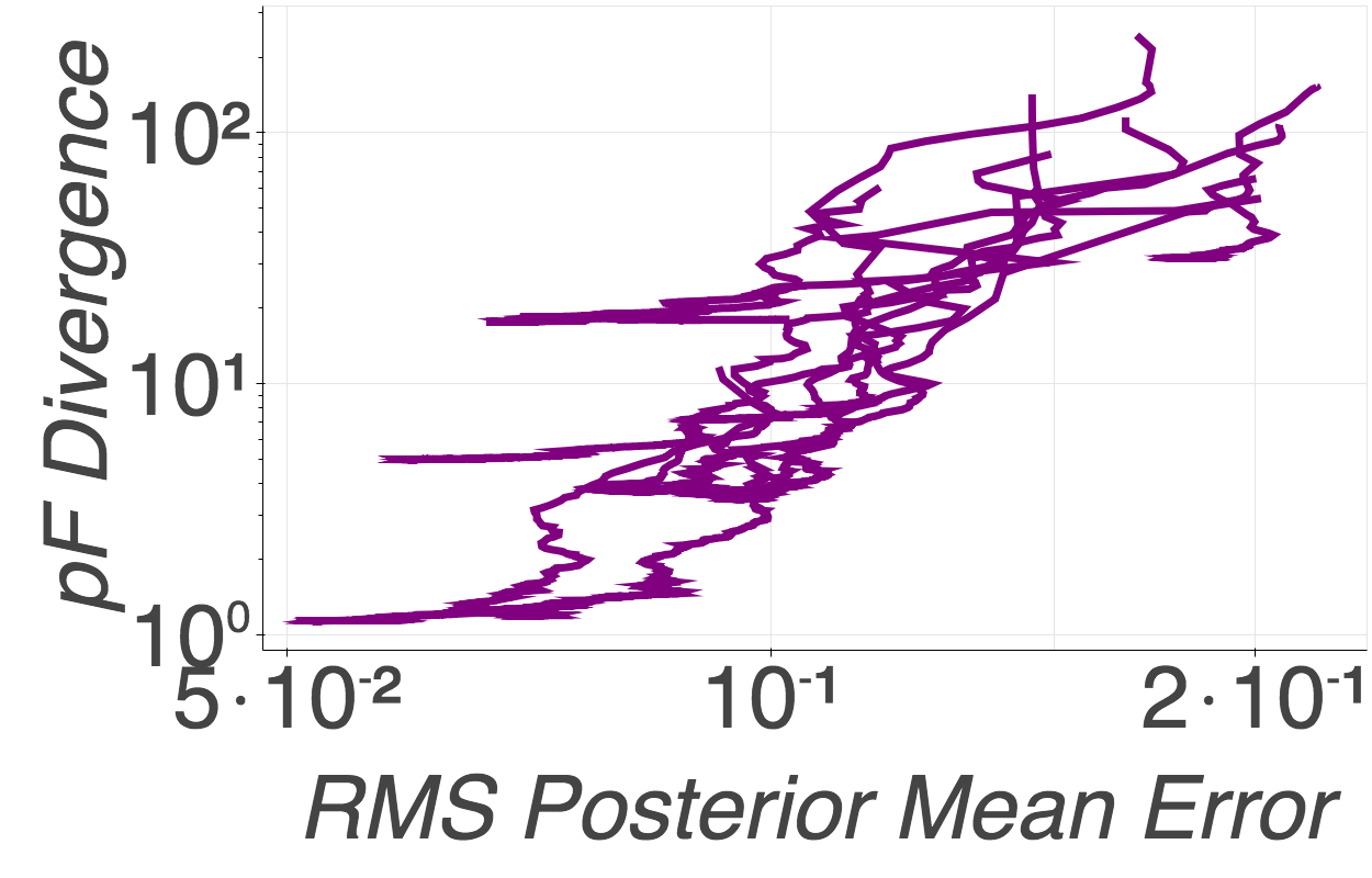
(b)

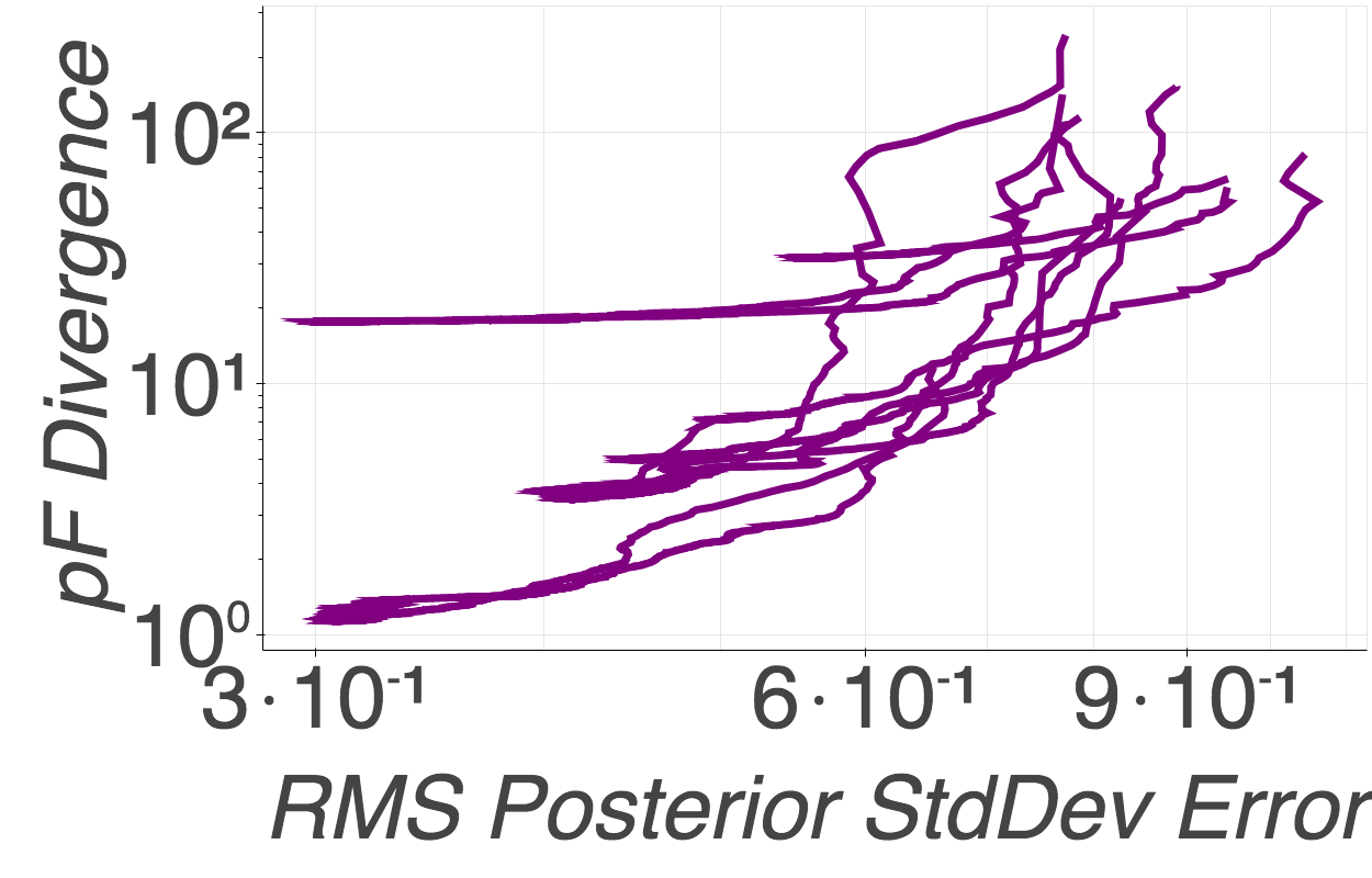
(c)

Figure 1: (a) Value of the pF-DTC objective on 10 runs for the airfoil data. (b,c) Relationship between the pF-DTC objective and the mean/standard deviation error on 10 runs for the airfoil dataset.

(a) pF-DTC

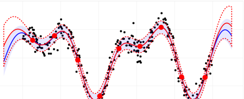
(b) VFE

(c) SoR

Figure 2: Comparison of pF-DTC, VFE, and SoR on the synthetic example with $M=9$ inducing points. Data is black, exact posterior mean and standard deviation are blue, and approximate fits and inducing points are red.

4.2 Choosing the auxiliary distribution

To apply Theorem 4.3, the auxiliary distribution $\nu$ must satisfy $\left\|{\mathrm{d}\pi/\mathrm{d}\nu}\right\|_{\infty}<\infty$. This finiteness condition is easy to achieve by letting $\nu={\mathrm{GP}}(\hat{\mu},\hat{k})$ and constructing $\hat{\mu}$ and $\hat{k}$ via a simple subset of datapoints approximation (Rasmussen and Williams, 2006, Ch. 8.3.3). Let $\hat{\bm{X}}\subset\bm{X}$ be a random subset of the input locations of size $M^{\prime}$, and take $\nu$ to be the GP posterior conditional on observing $\hat{\bm{y}}$, the subset of $\bm{y}$ corresponding to $\hat{\bm{X}}$. Therefore the auxiliary mean and covariance functions are $\hat{\mu}(\bm{x})=k_{\bm{x}\hat{\bm{X}}}[k_{\hat{\bm{X}}\hat{\bm{X}}}+\sigma^{2}I]^{-1}\hat{\bm{y}}$ and $\hat{k}(\bm{x},\bm{x}^{\prime})=k(\bm{x},\bm{x}^{\prime})-k_{\bm{x}\hat{\bm{X}}}[k_{\hat{\bm{X}}\hat{\bm{X}}}+\sigma^{2}I]^{-1}k_{\hat{\bm{X}}\bm{x}^{\prime}}$. Let $\hat{\bm{D}}=(\hat{\bm{X}},\hat{\bm{y}})$ denote the auxiliary data, and let $\mathcal{Z}_{{\bm{D}}}$ and $\mathcal{L}_{{\bm{D}}}$ denote the marginal likelihood and log-likelihood of the data ${\bm{D}}$ (with $\mathcal{Z}_{\hat{\bm{D}}}$ and $\mathcal{L}_{\hat{\bm{D}}}$ defined analogously). We can conclude that

$$\frac{\mathrm{d}\pi}{\mathrm{d}\nu}(f) =\frac{\mathcal{Z}_{\hat{\bm{D}}}e^{\mathcal{L}_{{\bm{D}}}(f)-\mathcal{L}_{\hat{\bm{D}}}(f)}}{\mathcal{Z}_{{\bm{D}}}}$$

$$=\frac{\mathcal{Z}_{\hat{\bm{D}}}e^{-\sum_{\bm{x}_{n}\in\bm{X}\setminus\hat{\bm{X}}}(f(\bm{x}_{n})-y_{n})^{2}/(2\sigma^{2})}}{(2\pi\sigma^{2})^{\frac{N-M^{\prime}}{2}}\mathcal{Z}_{{\bm{D}}}}$$

$$\leq\frac{\mathcal{Z}_{\hat{\bm{D}}}}{(2\pi\sigma^{2})^{\frac{N-M^{\prime}}{2}}\mathcal{Z}_{{\bm{D}}}}<\infty.$$

Hence Theorem 4.3 applies when the auxiliary distribution is a subset of datapoints approximation.

5 Preconditioned Fisher DTC

In this section we describe how to optimize the DTC inducing point approximation described in Section 2 using the pF divergence. We call the resulting inference algorithm preconditioned Fisher DTC (pF-DTC). Recall the DTC log-likelihood for the $n$th observation:

$$\tilde{\mathcal{L}}_{n}(f):=-\frac{1}{2\sigma^{2}}(k_{\bm{x}_{n}\bm{\tilde{X}}}k_{\bm{\tilde{X}}\bm{\tilde{X}}}^{-1}f_{\bm{\tilde{X}}}-y_{n})^{2}-\frac{1}{2}\log(2\pi\sigma^{2}).$$

We consider the case where $r=k$ at the locations of interest, which will simplify formulas (cf. Section 4.1). Let $Q_{\bm{X}\bm{X}}:=k_{\bm{X}\bm{\tilde{X}}}k_{\bm{\tilde{X}}\bm{\tilde{X}}}^{-1}k_{\bm{\tilde{X}}\bm{X}}$, $\bar{Q}_{\bm{X}\bm{\tilde{X}}}:=k_{\bm{X}\bm{\tilde{X}}}k_{\bm{\tilde{X}}\bm{\tilde{X}}}^{-1}$, and $S_{\bm{X}\bm{X}}:=Q_{\bm{X}\bm{X}}(I-(Q_{\bm{X}\bm{X}}+\sigma^{2}I)^{-1}Q_{\bm{X}\bm{X}})^{2}$. Our main result in this section provides a formula for computing the pF divergence in the sparse GP setting and guarantees that, up to a constant independent of the inducing points, $d_{\mathrm{pF},\nu}(\tilde{\pi}||\pi)$ can be computed efficiently.

Proposition 5.1.

For the DTC log-likelihood approximation, if $\nu={\mathrm{GP}}(\hat{\mu},\hat{k})$, then when $r=k$,

$$d_{\mathrm{pF},\nu}(\tilde{\pi}||\pi)$$

$$=\underbrace{\operatorname{Tr}((\hat{k}_{\bm{X}\bm{X}}+(\hat{\mu}_{\bm{X}}-\bm{y})(\hat{\mu}_{\bm{X}}-\bm{y})^{\top})(k_{\bm{X}\bm{X}}-Q_{\bm{X}\bm{X}}))}_{\mathrm{(I)}}$$

$$\phantom{=}+\underbrace{\operatorname{Tr}(\hat{k}_{\bm{X}\bm{X}}S_{\bm{X}\bm{X}})+\operatorname{Tr}(\hat{k}_{\bm{\tilde{X}}\bm{\tilde{X}}}\bar{Q}_{\bm{X}\bm{\tilde{X}}}^{\top}S_{\bm{X}\bm{X}}\bar{Q}_{\bm{X}\bm{\tilde{X}}})}_{\mathrm{(IIa)}}$$

$$\phantom{=}-\underbrace{2\operatorname{Tr}(\hat{k}_{\bm{\tilde{X}}\bm{X}}S_{\bm{X}\bm{X}}\bar{Q}_{\bm{X}\bm{\tilde{X}}})}_{\mathrm{(IIb)}}$$

$$\phantom{=}+\underbrace{(\hat{\mu}_{\bm{X}}-\bar{Q}_{\bm{X}\bm{\tilde{X}}}\hat{\mu}_{\bm{\tilde{X}}})^{\top}S_{\bm{X}\bm{X}}(\hat{\mu}_{\bm{X}}-\bar{Q}_{\bm{X}\bm{\tilde{X}}}\hat{\mu}_{\bm{\tilde{X}}})}_{\mathrm{(III)}}.$$

Furthermore, as long as vector multiplication by $\hat{k}_{\bm{X}\bm{X}}$ takes $O(NM)$ time, $d_{\mathrm{pF},\nu}(\tilde{\pi}||\pi)-C(\bm{X})$ can be computed in $O(NM^{2})$ time and $O(NM)$ space, where $C(\bm{X})$ is a function that does not depend on $\bm{\tilde{X}}$.

We can interpret the three terms in the expression for $d_{\mathrm{pF},\nu}(\tilde{\pi}||\pi)$ quite naturally. Term (I) measures how well the kernel matrix $k_{\bm{X}\bm{X}}$ is approximated by the Nyström approximation $Q_{\bm{X}\bm{X}}$. To interpret term (II) = (IIa) + (IIb), recall that the exact posterior kernel is $k_{{\bm{D}}}(\bm{x},\bm{x}^{\prime})=k(\bm{x},\bm{x}^{\prime})-k_{\bm{x}\bm{X}}[k_{\bm{X}\bm{X}}+\sigma^{2}I]^{-1}k_{\bm{X}\bm{x}^{\prime}}$. Observing the $(Q_{\bm{X}\bm{X}}+\sigma^{2}I)^{-1}$ terms in $S_{\bm{X}\bm{X}}$, we can see that term (II) measures how well the correction term $k_{\bm{x}\bm{X}}[k_{\bm{X}\bm{X}}+\sigma^{2}I]^{-1}k_{\bm{X}\bm{x}^{\prime}}$ is estimated. Finally, term (III) measures the quality of $\bar{Q}_{\bm{X}\bm{\tilde{X}}}\hat{\mu}_{\bm{\tilde{X}}}$, which is the inducing point approximation to the auxiliary mean function $\hat{\mu}_{\bm{X}}$. If we had to compute the terms in $d_{\mathrm{pF},\nu}(\tilde{\pi}||\pi)$ involving $k_{\bm{X}\bm{X}}$, then the time and space complexity would be, respectively, $O(MN^{2})$ and $O(N^{2})$. However, the terms that include $k_{\bm{X}\bm{X}}$ do not depend on the inducing points, so we absorb them into $C(\bm{X})$.

6 Experiments

Our theory shows that pF-DTC can provide guarantees on the quality of the approximate GP posterior means and variances that practitioners typically report (Section 1). We now check empirically that our method yields competitive estimates of exact GP means and variances in practice. We compare pF-DTC to to variational DTC (VFE) (Titsias, 2009), subset of regressors (SoR) (Smola and Bartlett, 2000), and exact GP inference with a random subsample of the data (subsample). To compare to the exact GP as ground truth, all experiments use the same kernel (squared exponential kernel with separate length scales for each dimension) and identical hyperparameters. To that end, unless noted otherwise, we fix the kernel hyperparameters and the observation noise $\sigma^{2}$, all of which we learn with a pilot run of VFE using 200 fixed randomly chosen inducing points. We found that if we optimized the hyperparameters for pF-DTC and VFE after inducing point optimization, they remained relatively stable. For pF-DTC we take $r=k$, as justified by Proposition 4.5. Although constructing $\nu$ from a subset of data is currently the most justified choice theoretically (see Section 4.2), preliminary experiments showed better empirical performance using SoR with a small random subset of the data.

We used one synthetic and five real datasets with dimensionality ranging from 1 to 11. In order to run the exact GP on all datasets we subsampled the original airline delays dataset used by Hensman et al. (2013) down to 10,000 observations. The remaining non-synthetic datasets were obtained from the UCI Machine Learning Repository. We held out the maximum of 1,000 observations or 20% of each dataset for testing and used the remainder for training (training set sizes were between 1,000 and 8,000). See Appendix A in Appendix A for full details. We repeated all experiments 10 times.

Behavior of the pF divergence. The pF-DTC objective is non-convex, so we first check that we can effectively optimize it. As seen in Fig. 1(a), for the airfoil dataset, optimizing the locations of the 200 inducing points substantially reduces the size of the pF divergence, though clearly we are finding only local optima. The bounds in Theorem 4.3 suggest a linear relationship between the pF divergence and the errors in estimates of the posterior mean $\mu_{{\bm{D}}}(\bm{x})$ and standard deviation $k_{{\bm{D}}}(\bm{x},\bm{x})^{1/2}$. Figs. 1(b) and 1(c) show an approximately linear relationship does in fact hold in both cases.

NOTUSED

(a) synthetic

(b) delays10k

(c) abalone

(d) airfoil

(e) CCPP

(f) wine

Figure 3: Root mean squared error of the approximate posterior mean (left) and standard deviation (right) at the held-out test locations.

(a) synthetic

(b) delays10k

(c) abalone

(d) airfoil

(e) CCPP

(f) wine

Figure 4: Predictive performance as measured by root mean squared error.

Mean and Variance Estimates. We first consider a simple one-dimensional synthetic example to compare pF-DTC to VFE and SoR. Fig. 2 shows that, with 9 inducing points, pF-DTC and VFE produce excellent, almost identical fits, while SoR performs substantially worse at estimating both the posterior mean and standard deviation. Bauer et al. (2016) found similarly poor performance for the fully independence training conditional (FITC) method of Snelson and Ghahramani (2005).

On more complex problems, we consider root mean squared error (RMSE) of posterior mean and standard deviation estimates at all held-out test locations, as we vary the number of inducing points. Fig. 7 confirms that pF-DTC is competitive with VFE, validating the practicality of the pF divergence as an objective for approximate inference. VFE shows better performance for larger numbers of inducing points once the error dips below $10^{-3}$, which we suspect is related to numerical issues. SoR shows surprisingly good performance on standard deviation error but worse mean estimation—particularly on abalone. As expected, subsampling performed poorly.

KL divergence and comparison of objective functions. In Section 3 we argued that KL divergence is a suboptimal way to measure posterior approximation quality when the goal is good posterior mean and standard deviation estimates. We here show that this issue arises in practice. Figs. 6, A.2 and A.1 show the KL divergences for all four approximations. We see that VFE sometimes yields small KL divergence but worse posterior mean and standard deviation estimates. Similarly, we see that pF-DTC can exhibit larger KL divergence values but very good posterior mean and standard deviation estimates.

Predictive Performance. While our focus in this paper is on posterior mean and variance estimates, we also used the held-out test data to check RMSE predictive performance. As shown in Fig. 5, pF-DTC, SoR, and VFE performed quite similarly, with subsampling providing worse predictive accuracy.

Computation. In over 80% of our 60 experiments (10 experiments per dataset), pF-DTC used less computation than VFE. On average, VFE was 4.5 times slower than pF-DTC. Because they did not involve any optimization, SoR and subsample were orders of magnitude faster.

7 Discussion

In this paper we have developed an approach to scalable Gaussian process regression using a novel objective, the preconditioned Fisher divergence, which we show bounds the 2-Wasserstein distance. We were motivated by the need to guarantee the finite-data accuracy of posterior mean and covariance function estimates. Empirically we showed that using the pF divergence with a DTC likelihood approximation provides competitive mean and variance estimates with state-of-the-art approaches.

The current work demonstrates the feasibility of using the pF divergence, but there are many important directions for future work. The first is to scale to larger datasets, e.g. using stochastic optimization techniques similar in spirit to SVI for GPs (Hensman et al., 2013). A second direction is to use the pF divergence objective with other likelihood approximations. Structured kernel approximations are of particular interest since these are both fast to compute and can often better capture multi-scale structure (Wilson and Nickisch, 2015; Gardner et al., 2018). Finally, it remains to efficiently utilize the preconditioned Fisher divergence for other likelihoods, such as in GP classification.

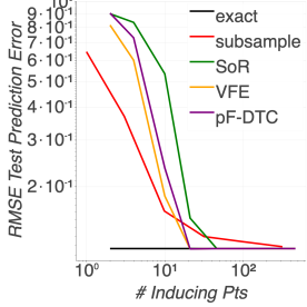
(a) synthetic

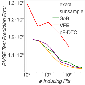
(b) delays10k

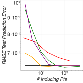
(c) abalone

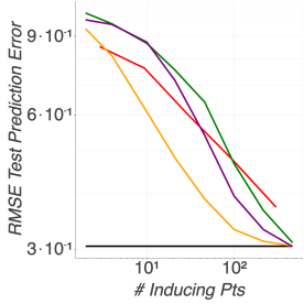
(d) airfoil

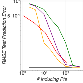
(e) CCPP

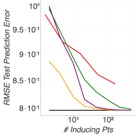
(f) wine

Figure 5: Predictive performance as measured by root mean squared error.

(a) airfoil

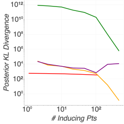
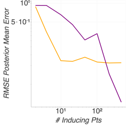
(b) CCPP

Figure 6: KL divergences of the approximate posteriors and root mean squared error of the approximate posteriors for the VFE and pF-DTC trials with the smallest objective values.

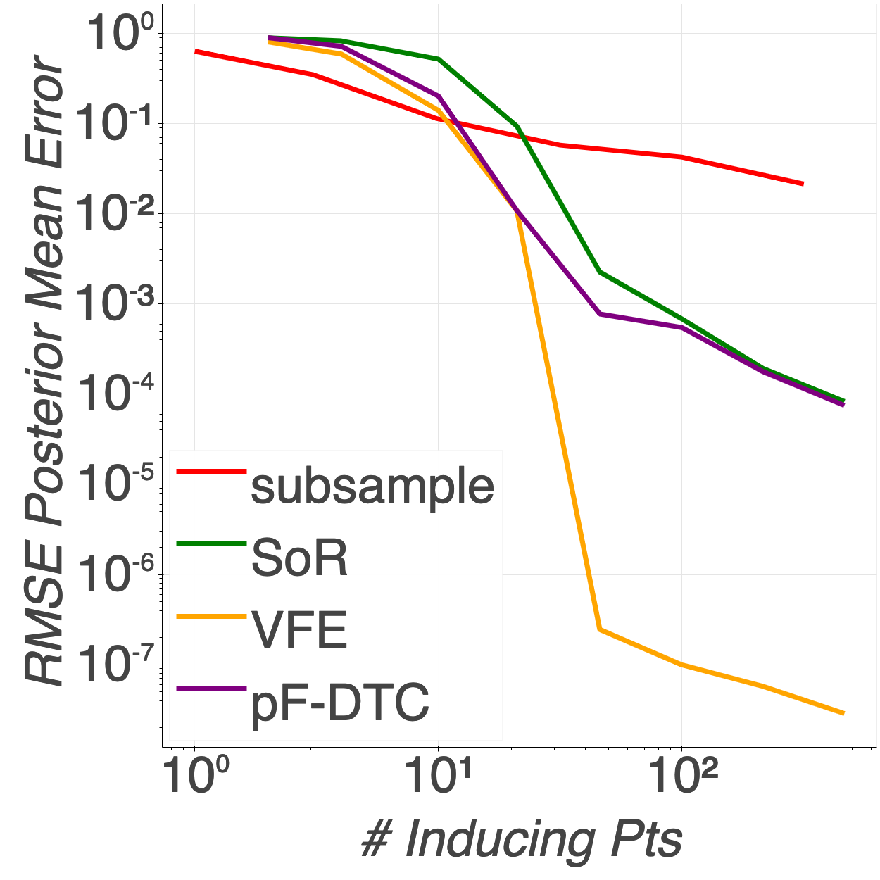
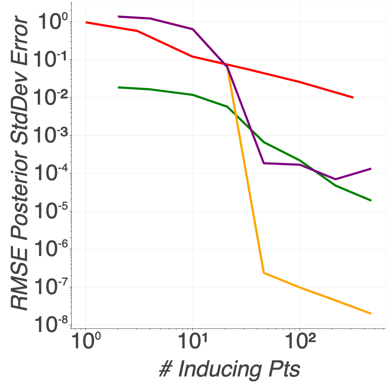
(a) synthetic

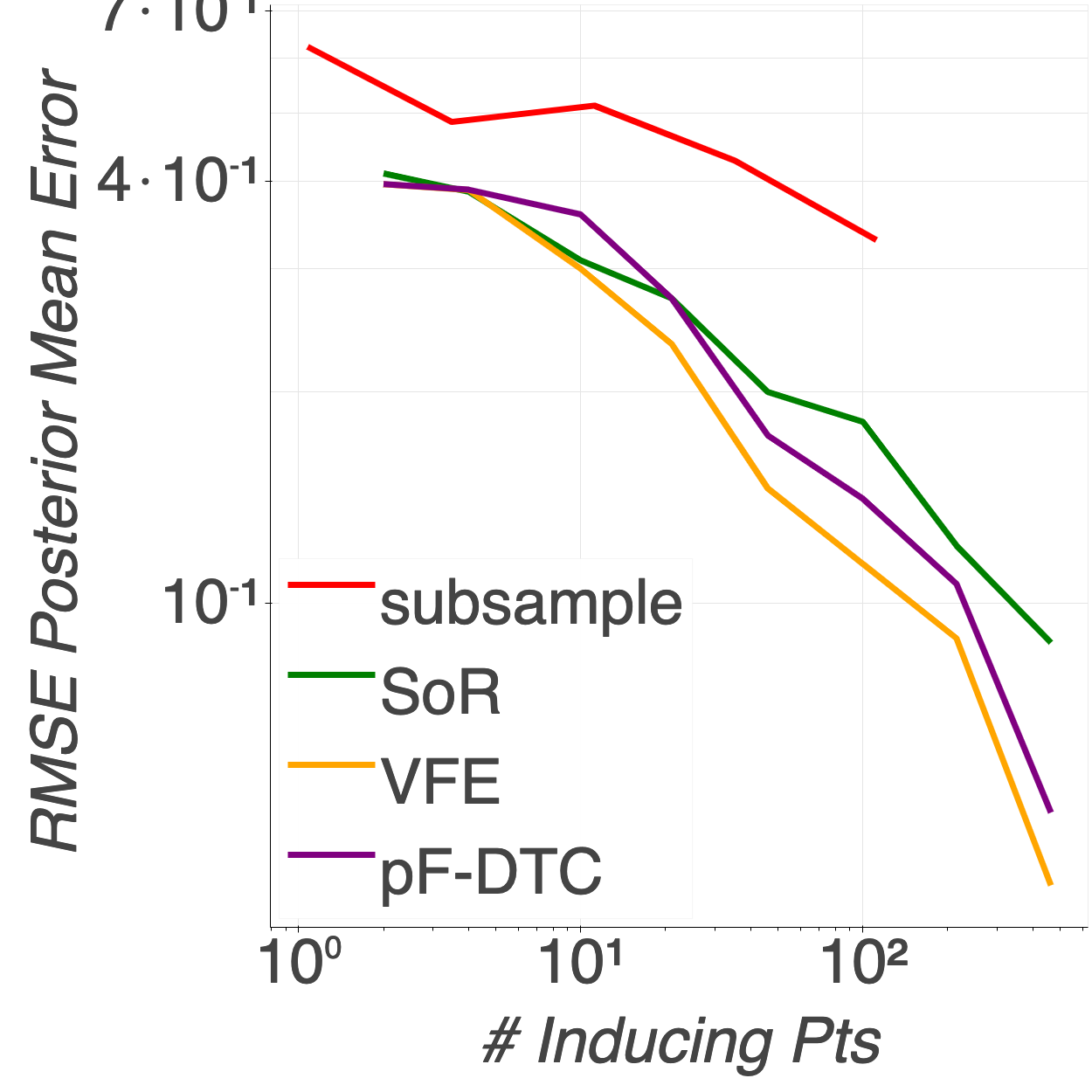
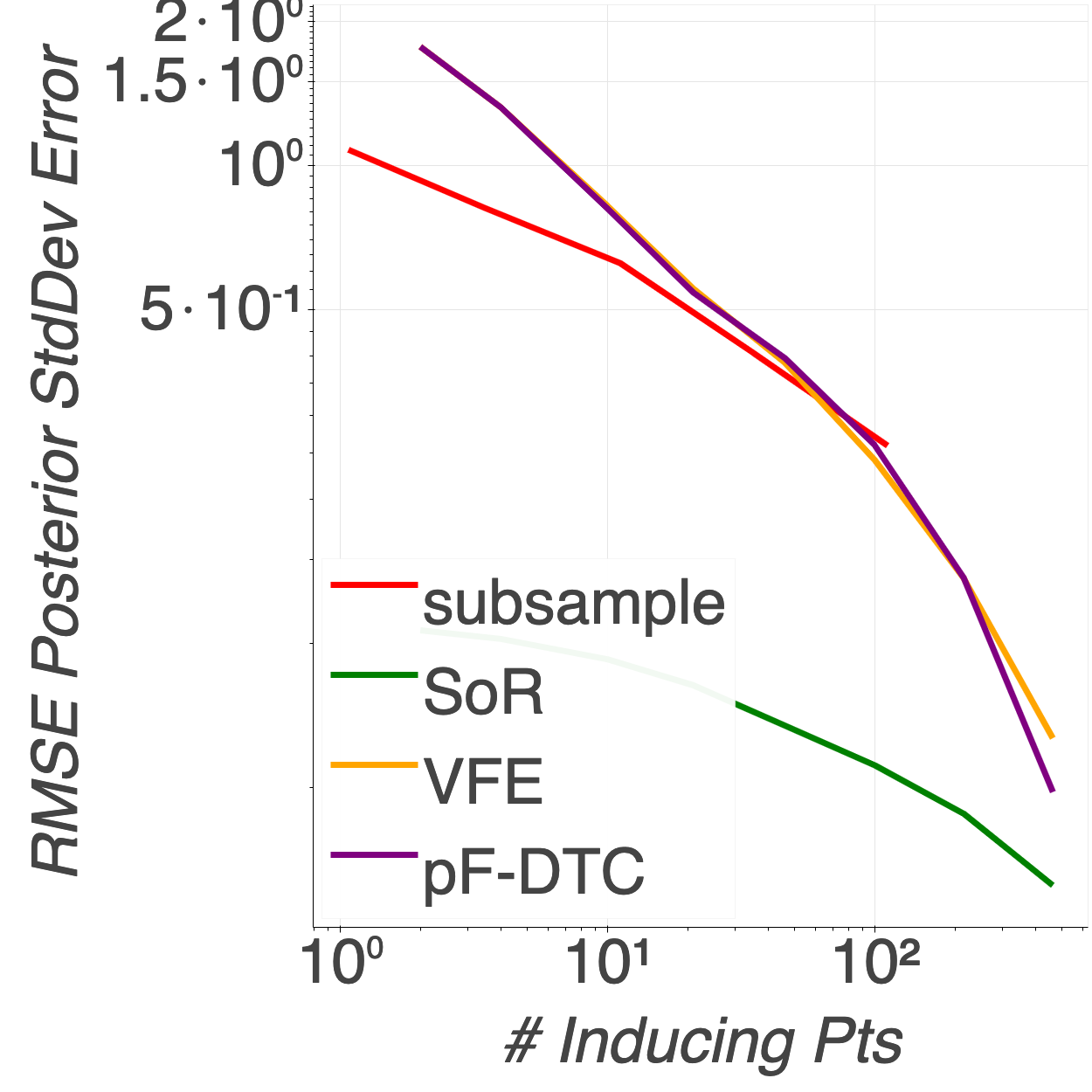
(b) delays10k

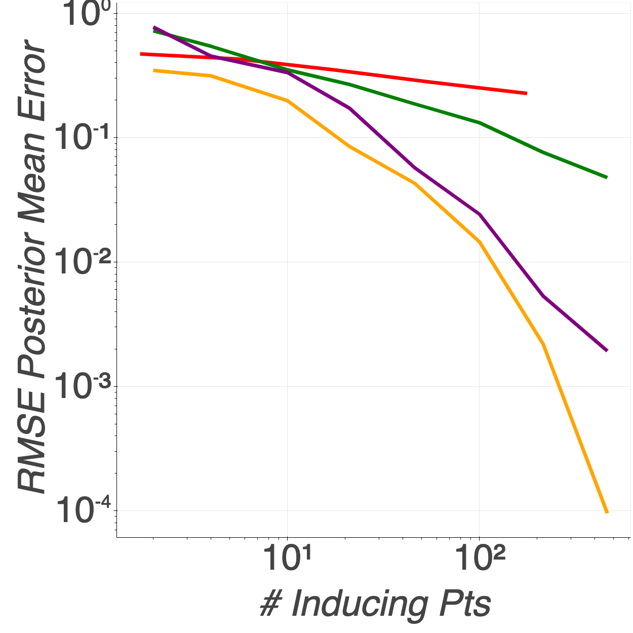
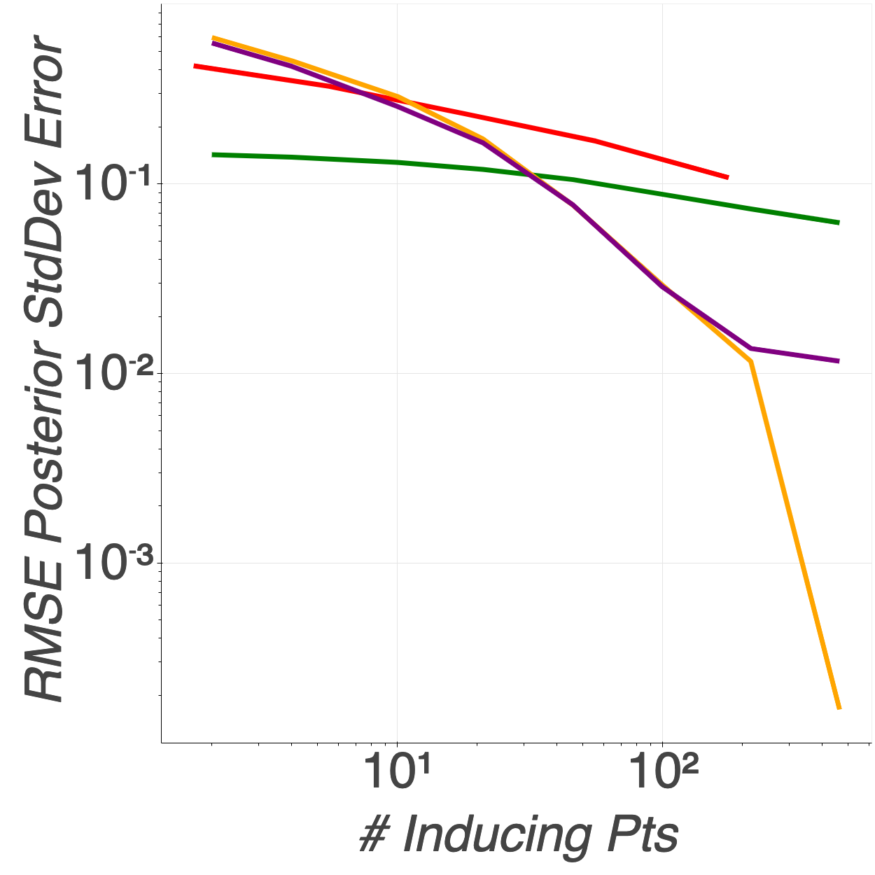
(c) abalone

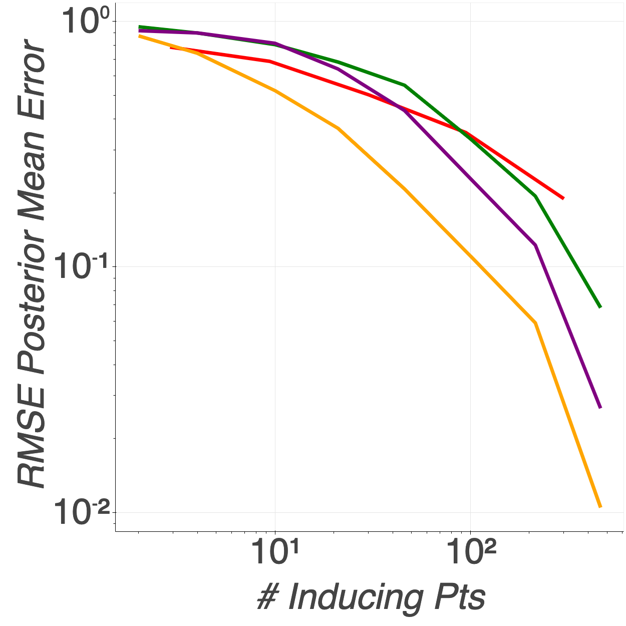
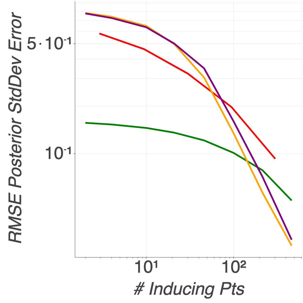
(d) airfoil

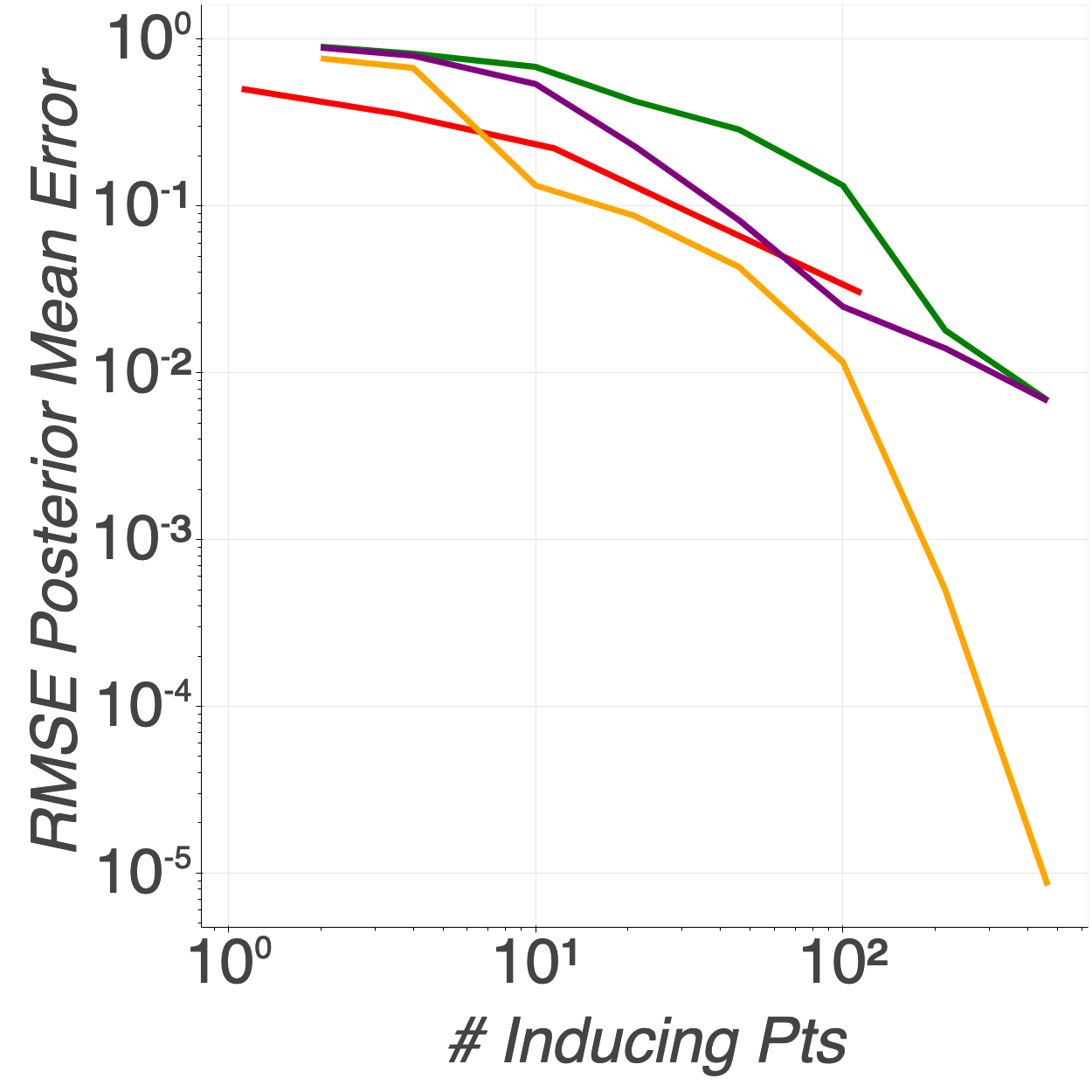
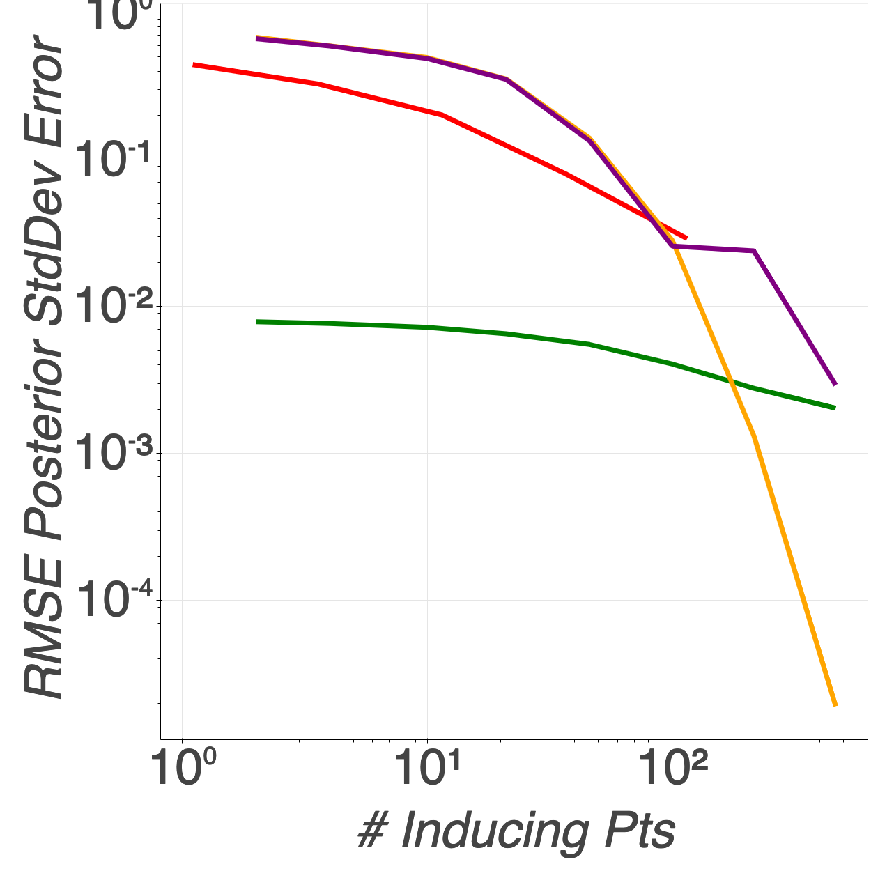
(e) CCPP

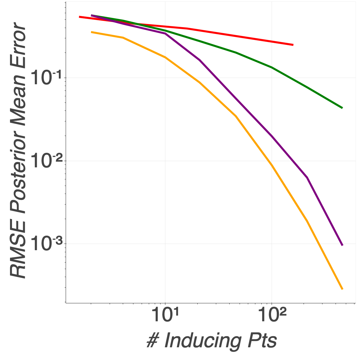
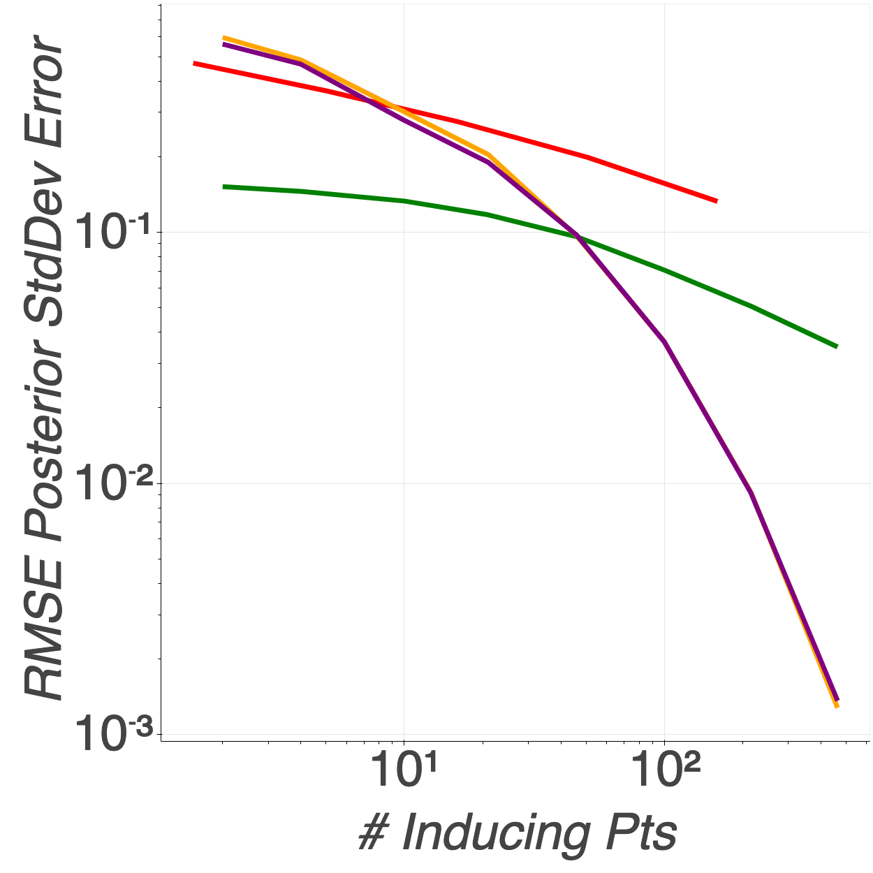
(f) wine

Figure 7: Root mean squared error of the approximate posterior mean (left) and standard deviation (right) at the held-out test locations.

Acknowledgments

Thanks to Nicolo Fusi for helpful discussions. Thanks to Dan Simpson and Arthur Gretton for valuable feedback on an earlier draft of this paper. This research was supported in part by an NSF CAREER Award, an ARO YIP Award, the Office of Naval Research, a Sloan Research Fellowship, IBM, and Amazon. M. Kasprzak was supported by an EPSRC studentship.

arxiv

Appendix

Appendix A Experiments

Datasets used for experiments. All datasets from the UCI Machine Learning Repository^a except for synthetic and delays10k datasets.
$K=$ number of datapoints used to construct $\nu$ (approximately 10% of $N_{\text{train}}$) Name $N_{\text{train}}$ $N_{\text{test}}$ $d$ $K$ Name $N_{\text{train}}$ $N_{\text{test}}$ $d$ $K$ synthetic 1000 1000 1 100 abalone 3177 1000 8 300 delays10k^b 8000 2000 8 800 airfoil 1103 400 5 100 CCPP 7568 2000 4 700 wine quality 3898 1000 11 300

• http://archive.ics.uci.edu/ml/index.php

• Hensman et al. (2013)

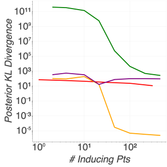
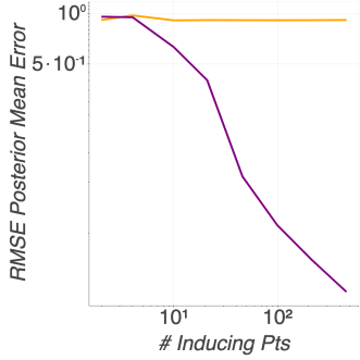
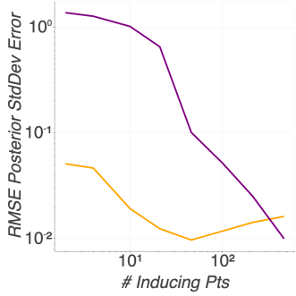
(a) synthetic

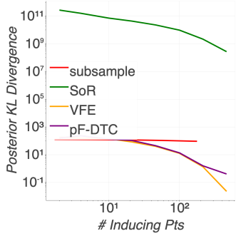
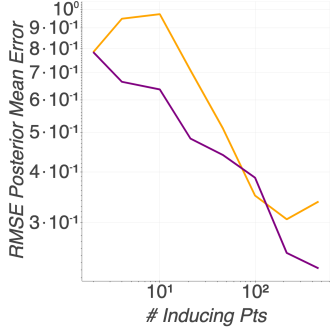
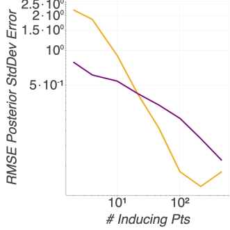
(b) abalone

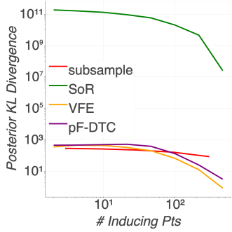
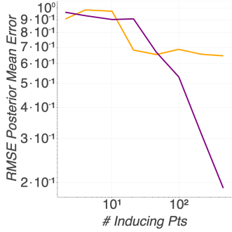
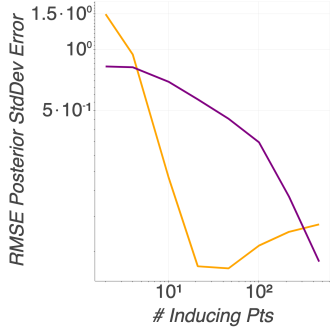
(c) airfoil

Figure A.1: KL divergences of the approximate posteriors and root mean squared error of the approximate posteriors for the VFE and pF-DTC trials with the smallest objective values.

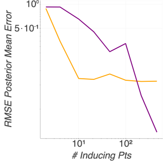
(a) CCPP

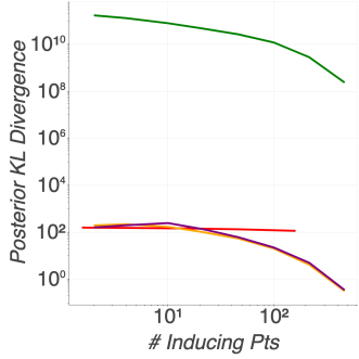
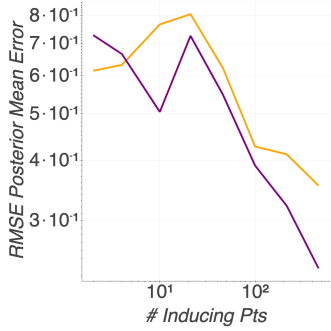
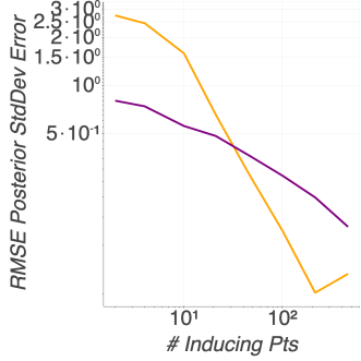
(b) wine

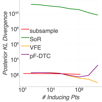
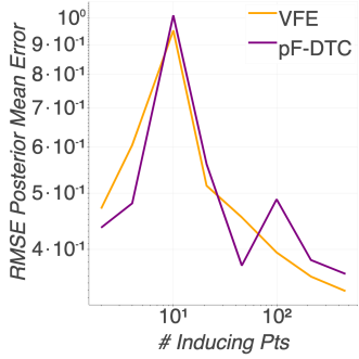
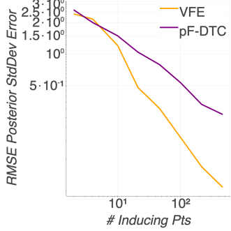
(c) delays10k

Figure A.2: KL divergences of the approximate posteriors and root mean squared error of the approximate posteriors for the VFE and pF-DTC trials with the smallest objective values.

Appendix B Proof of Proposition 3.1

Choose the means and variances of $\eta$ and $\tilde{\eta}$ such that $(\tilde{\mu}-\mu)^{2}=\tilde{s}^{2}\{\exp(2\delta)-1\}$ and $s^{2}=\exp(2\delta)\tilde{s}^{2}$. We then have that

$$\mathrm{KL}(\tilde{\eta}||\eta)$$

$$=0{\cdot}5\{\tilde{s}^{2}/s^{2}-1+\log(s^{2}/\tilde{s}^{2})+(\tilde{\mu}-\mu)^{2}/s^{2}\}$$

$$=0{\cdot}5[\tilde{s}^{2}/\{\exp(2\delta)\tilde{s}^{2}\}-1+\log\{\exp(2\delta)\tilde{s}^{2}/\tilde{s}^{2}\}+\tilde{s}^{2}\{\exp(2\delta)-1\}/\{\exp(2\delta)\tilde{s}^{2}\}]$$

$$=0{\cdot}5[\exp(-2\delta)-1+\log\{\exp(2\delta)\}+\{\exp(2\delta)-1\}\exp(-2\delta)]$$

$$=\delta.$$

Appendix C Details of 4.1

We take $\mathbb{H}$ to be the reproducing kernel Hilbert space with reproducing kernel $r$. The posterior covariance functions for $\eta$ and $\tilde{\eta}$ are equal to

$$k_{{\bm{D}}}(x,x^{\prime})=e^{-(x-x^{\prime})^{2}/2}-(1+\sigma^{2})^{-1}e^{-x^{2}/2-(x^{\prime})^{2}/2}$$ (C.1)

while their posterior means are, respectively, $\mu(x)=(1+\sigma^{2})^{-1}e^{-x^{2}/2}t$ and $\tilde{\mu}(x)=(1+\sigma^{2})^{-1}e^{-x^{2}/2}\tilde{t}$ Define the induced kernel $k^{\prime}(x,x^{\prime}):=\langle{k_{x}},{k_{x^{\prime}}}\rangle$. Since their covariance operators are equal, the 2-Wasserstein distance between the $\eta$ and $\tilde{\eta}$ is (Gelbrich, 1990, Thm. 3.5)

$$\mathcal{W}_{2}(\eta,\tilde{\eta}) =\left\|{\mu-\tilde{\mu}}\right\|=\left\|{k(0,\cdot)}\right\|(1+\sigma^{2})^{-1}|t-\tilde{t}|$$

$$=\mathchoice{{\hbox{$\displaystyle\sqrt{k^{\prime}(0,0)\,}$}\lower 0.4pt\hbox{\vrule height=8.5pt,depth=-6.80003pt}}}{{\hbox{$\textstyle\sqrt{k^{\prime}(0,0)\,}$}\lower 0.4pt\hbox{\vrule height=8.5pt,depth=-6.80003pt}}}{{\hbox{$\scriptstyle\sqrt{k^{\prime}(0,0)\,}$}\lower 0.4pt\hbox{\vrule height=5.97221pt,depth=-4.7778pt}}}{{\hbox{$\scriptscriptstyle\sqrt{k^{\prime}(0,0)\,}$}\lower 0.4pt\hbox{\vrule height=4.58333pt,depth=-3.66669pt}}}(1+\sigma^{2})^{-1}|t-\tilde{t}|.$$ (C.2)

The log-likelihoods associated with $\eta$ and $\tilde{\eta}$ are, respectively, $\mathcal{L}(f):=-\frac{1}{2\sigma^{2}}(f(0)-t)^{2}$ and $\tilde{\mathcal{L}}(f):=-\frac{1}{2\sigma^{2}}(f(0)-\tilde{t})^{2}$. Using Lemma F.3, in the non-preconditioned case we have

$$d_{\mathrm{F},\nu}(\eta,\tilde{\eta})^{2} =\mathbb{E}_{f\sim\nu}[\langle{\mathcal{D}\mathcal{L}},{\mathcal{D}\mathcal{L}}\rangle+\langle{\mathcal{D}\tilde{\mathcal{L}}},{\mathcal{D}\tilde{\mathcal{L}}}\rangle-2\langle{\mathcal{D}\mathcal{L}},{\mathcal{D}\tilde{\mathcal{L}}}\rangle]$$

$$=\sigma^{-4}r(0,0)[(t-\hat{\mu}(0))^{2}+(\tilde{t}-\hat{\mu}(0))^{2}-2(t-\hat{\mu}(0))(\tilde{t}-\hat{\mu}(0))]$$

$$=\sigma^{-4}r(0,0)(t-\tilde{t})^{2}.$$ (C.3)

Eqs. C.2 and C.3 together show that $c=\mathchoice{{\hbox{$\displaystyle\sqrt{r(0,0)/k^{\prime}(0,0)\,}$}\lower 0.4pt\hbox{\vrule height=8.5pt,depth=-6.80003pt}}}{{\hbox{$\textstyle\sqrt{r(0,0)/k^{\prime}(0,0)\,}$}\lower 0.4pt\hbox{\vrule height=8.5pt,depth=-6.80003pt}}}{{\hbox{$\scriptstyle\sqrt{r(0,0)/k^{\prime}(0,0)\,}$}\lower 0.4pt\hbox{\vrule height=5.97221pt,depth=-4.7778pt}}}{{\hbox{$\scriptscriptstyle\sqrt{r(0,0)/k^{\prime}(0,0)\,}$}\lower 0.4pt\hbox{\vrule height=4.58333pt,depth=-3.66669pt}}}$.

The preconditioned case is almost identical to Eq. C.3. Using Lemmas F.1, F.4 and C.1, for any $f\in\mathbb{H}$,

$$\mathcal{C}_{\tilde{\eta}}\mathcal{D}\mathcal{L}(f) =-(1+\sigma^{2})^{-1}(f(0)-t)k(0,\cdot)$$

and similarly for $\mathcal{C}_{\tilde{\eta}}\mathcal{D}\tilde{\mathcal{L}}(f)$. Hence,

$$d_{\mathrm{pF},\nu}(\eta||\tilde{\eta}) =\mathbb{E}_{f\sim\nu}[\langle{\mathcal{C}_{\tilde{\eta}}\mathcal{D}\mathcal{L}},{\mathcal{C}_{\tilde{\eta}}\mathcal{D}\mathcal{L}}\rangle+\langle{\mathcal{C}_{\tilde{\eta}}\mathcal{D}\tilde{\mathcal{L}}},{\mathcal{C}_{\tilde{\eta}}\mathcal{D}\tilde{\mathcal{L}}}\rangle-2\langle{\mathcal{C}_{\tilde{\eta}}\mathcal{D}\mathcal{L}},{\mathcal{C}_{\tilde{\eta}}\mathcal{D}\tilde{\mathcal{L}}}\rangle]$$

$$=(1+\sigma^{2})^{-2}k^{\prime}(0,0)[(t-\hat{\mu}(0))^{2}+(\tilde{t}-\hat{\mu}(0))^{2}-2(t-\hat{\mu}(0))(\tilde{t}-\hat{\mu}(0))]$$

$$=(1+\sigma^{2})^{-2}k^{\prime}(0,0)(t-\tilde{t})^{2}.$$ (C.4)

Eqs. C.2 and C.4 together show that $d_{\mathrm{pF},\nu}(\eta||\tilde{\eta})=\mathcal{W}_{2}(\eta,\tilde{\eta}).$

Appendix D Proof of Theorem 4.3

Theorem 4.3 will follow almost immediately after we develop a number of preliminary results. For more details on infinite-dimensional SDEs and related ideas, we recommend Hairer et al. (2005, 2007) and Da Prato and Zabczyk (2014).

The notation in this section differs slightly from the rest of the paper in order to follow the conventions of the stochastic processes literature. Let $W$ denote a $\mathcal{C}$-Wiener process (Da Prato and Zabczyk, 2014, Definition 4.2), where $\mathcal{C}:\mathbb{H}\to\mathbb{H}$ is the linear, self-adjoint, positive semi-definite, trace-class operator. Let $\mu\in\mathbb{H}$ and let $b,\tilde{b}:\mathbb{H}\to\mathbb{R}$ and consider the following infinite-dimensional stochastic differential equations (SDEs) in $\mathbb{H}$ :

$$\mathrm{d}X_{t} =(\mu-X_{t})\mathrm{d}t+b(X_{t})\mathrm{d}t+\mathchoice{{\hbox{$\displaystyle\sqrt{2\,}$}\lower 0.4pt\hbox{\vrule height=6.44444pt,depth=-5.15558pt}}}{{\hbox{$\textstyle\sqrt{2\,}$}\lower 0.4pt\hbox{\vrule height=6.44444pt,depth=-5.15558pt}}}{{\hbox{$\scriptstyle\sqrt{2\,}$}\lower 0.4pt\hbox{\vrule height=4.51111pt,depth=-3.6089pt}}}{{\hbox{$\scriptscriptstyle\sqrt{2\,}$}\lower 0.4pt\hbox{\vrule height=3.22221pt,depth=-2.57779pt}}}\mathrm{d}W_{t}$$ (D.1)

$$\mathrm{d}Y_{t} =(\mu-Y_{t})\mathrm{d}t+\tilde{b}(Y_{t})\mathrm{d}t+\mathchoice{{\hbox{$\displaystyle\sqrt{2\,}$}\lower 0.4pt\hbox{\vrule height=6.44444pt,depth=-5.15558pt}}}{{\hbox{$\textstyle\sqrt{2\,}$}\lower 0.4pt\hbox{\vrule height=6.44444pt,depth=-5.15558pt}}}{{\hbox{$\scriptstyle\sqrt{2\,}$}\lower 0.4pt\hbox{\vrule height=4.51111pt,depth=-3.6089pt}}}{{\hbox{$\scriptscriptstyle\sqrt{2\,}$}\lower 0.4pt\hbox{\vrule height=3.22221pt,depth=-2.57779pt}}}\mathrm{d}W_{t}.$$ (D.2)

We will need the constructions from the following lemma, the proof of which is deferred to Section D.1.

Lemma D.1.

Let $\tilde{\mathbb{H}}:=\mathbb{H}\oplus\mathbb{H}$, the direct sum of $\mathbb{H}$ with itself, for which the inner product is given by

$$\langle{(x_{1},x_{2})},{(y_{1},y_{2})}\rangle_{\tilde{\mathbb{H}}}=\langle{x_{1}},{y_{1}}\rangle+\langle{x_{2}},{y_{2}}\rangle.$$

Define the self-adjoint operator $\tilde{\mathcal{C}}:\tilde{\mathbb{H}}\to\tilde{\mathbb{H}}$ given by $(x,y)\mapsto(\mathcal{C}(x+y),\mathcal{C}(x+y))$. Then Eqs. D.1 and D.2 can be written on a common probability space as

$$\mathrm{d}(X_{t},Y_{t})=(\mu,\mu)\mathrm{d}t-(X_{t},Y_{t})\mathrm{d}t+(b(X_{t}),\tilde{b}(Y_{t}))\mathrm{d}t+\mathchoice{{\hbox{$\displaystyle\sqrt{2\,}$}\lower 0.4pt\hbox{\vrule height=6.44444pt,depth=-5.15558pt}}}{{\hbox{$\textstyle\sqrt{2\,}$}\lower 0.4pt\hbox{\vrule height=6.44444pt,depth=-5.15558pt}}}{{\hbox{$\scriptstyle\sqrt{2\,}$}\lower 0.4pt\hbox{\vrule height=4.51111pt,depth=-3.6089pt}}}{{\hbox{$\scriptscriptstyle\sqrt{2\,}$}\lower 0.4pt\hbox{\vrule height=3.22221pt,depth=-2.57779pt}}}\mathrm{d}(W_{t},W_{t})$$ (D.3)

or

$$(X_{t},Y_{t})=\int_{0}^{t}(\mu,\mu)\mathrm{d}s-\int_{0}^{t}(X_{s},Y_{s})\mathrm{d}s+\int_{0}^{t}(b(X_{s}),\tilde{b}(Y_{s}))\mathrm{d}s+\mathchoice{{\hbox{$\displaystyle\sqrt{2\,}$}\lower 0.4pt\hbox{\vrule height=6.44444pt,depth=-5.15558pt}}}{{\hbox{$\textstyle\sqrt{2\,}$}\lower 0.4pt\hbox{\vrule height=6.44444pt,depth=-5.15558pt}}}{{\hbox{$\scriptstyle\sqrt{2\,}$}\lower 0.4pt\hbox{\vrule height=4.51111pt,depth=-3.6089pt}}}{{\hbox{$\scriptscriptstyle\sqrt{2\,}$}\lower 0.4pt\hbox{\vrule height=3.22221pt,depth=-2.57779pt}}}(W_{t},W_{t}),$$ (D.4)

where $t\mapsto(X_{t},Y_{t})$ is a process on $\tilde{\mathbb{H}}$ and $t\mapsto(W_{t},W_{t})$ is a $\tilde{\mathcal{C}}$-Wiener process on $\tilde{\mathbb{H}}$.

Let $\mathcal{P}$ denote the space of Borel measures on $\mathbb{H}$. Recall that for any $\eta\in\mathcal{P}$, the $\left\|{\cdot}\right\|_{\eta}$-norm acting on functions $A:\mathbb{H}\to\mathbb{H}$ is defined by

$$\left\|{A}\right\|_{\eta}:=\left(\int\left\|{A(x)}\right\|^{2}\eta(\mathrm{d}x)\right)^{1/2}.$$

Theorem D.2.

Assume that Eq. D.3 has a unique stationary law with the marginal stationary laws of Eqs. D.1 and D.2 given by $\tilde{\eta}$ and $\eta$ respectively. Suppose that for $X\sim\tilde{\eta}$ and $Y\sim\eta$, $\mathbb{E}\left\|{X}\right\|^{2}<\infty$ and $\mathbb{E}\left\|{Y}\right\|^{2}<\infty$. Suppose that for some $\alpha>0$, $b$ satisfies the one-sided Lipschitz condition

$$\langle{b(x)-b(y)},{x-y}\rangle\leq(-\alpha+1)\left\|{x-y}\right\|^{2}\text{ for all }x,y\in\mathbb{H}.$$ (D.5)

Then

$$\mathcal{W}_{2}(\eta,\tilde{\eta})\leq\alpha^{-1}\|{b-\tilde{b}}\|_{\eta}.$$ (D.6)

We defer the proof to Section D.2.

Proposition D.3.

If the hypotheses of Theorem D.2 hold, then for any distribution $\nu\in\mathcal{P}$ such that $\nu\ll\eta$,

$$\mathcal{W}_{2}(\eta,\tilde{\eta})\leq\alpha^{-1}\left\|{\frac{\mathrm{d}\eta}{\mathrm{d}\nu}}\right\|_{\infty}^{1/2}\|{b-\tilde{b}}\|_{\nu}$$ (D.7)

Proof.

Using Hölder’s inequality, we have

$$\|{b-\tilde{b}}\|_{\eta}^{2} =\int\|{b(x)-\tilde{b}(x)}\|^{2}\eta(\mathrm{d}x)$$

$$=\int\frac{\mathrm{d}\eta}{\mathrm{d}\nu}(x)\|{b(x)-\tilde{b}(x)}\|^{2}\nu(\mathrm{d}x)$$

$$\leq\left\|{\frac{\mathrm{d}\eta}{\mathrm{d}\nu}}\right\|_{\infty}\int\|{b(x)-\tilde{b}(x)}\|^{2}\nu(\mathrm{d}x).$$

Eq. D.7 follows by plugging the previous display into Eq. D.6. ∎

Proposition D.4.

If $\eta,\nu\in\mathcal{P}$, $\mathcal{W}_{2}(\eta,\nu)\leq\varepsilon$ and $\mathbb{H}=\mathbb{H}_{r}$, then for all $\bm{x}\in\mathcal{X}$,

$$|\mu_{\eta}(\bm{x})-\mu_{\nu}(\bm{x})| \leq r(\bm{x},\bm{x})^{1/2}\varepsilon$$

$$|k_{\eta}(\bm{x},\bm{x})^{1/2}-k_{\nu}(\bm{x},\bm{x})^{1/2}| \leq\mathchoice{{\hbox{$\displaystyle\sqrt{6\,}$}\lower 0.4pt\hbox{\vrule height=6.44444pt,depth=-5.15558pt}}}{{\hbox{$\textstyle\sqrt{6\,}$}\lower 0.4pt\hbox{\vrule height=6.44444pt,depth=-5.15558pt}}}{{\hbox{$\scriptstyle\sqrt{6\,}$}\lower 0.4pt\hbox{\vrule height=4.51111pt,depth=-3.6089pt}}}{{\hbox{$\scriptscriptstyle\sqrt{6\,}$}\lower 0.4pt\hbox{\vrule height=3.22221pt,depth=-2.57779pt}}}r(\bm{x},\bm{x})^{1/2}\varepsilon$$

$$|k_{\eta}(\bm{x},\bm{x})-k_{\nu}(\bm{x},\bm{x})| \leq 3\,r(\bm{x},\bm{x})^{1/2}\min(k_{\eta}(\bm{x},\bm{x}),k_{\nu}(\bm{x},\bm{x}))^{1/2}\varepsilon+6\,r(\bm{x},\bm{x})\varepsilon^{2}.$$

We defer the proof to Section D.3.

The result will follow by taking $\mathcal{C}=\mathcal{C}_{\tilde{\eta}}$. With this choice of $\mathcal{C}$, $b=0$ and $\mu=\mu_{\tilde{\eta}}$, so $b$ satisfies the one-sided Lipschitz condition with $\alpha=1$. The remaining hypotheses of Theorem D.2 hold by construction, so Theorem 4.3 follows by applying Propositions D.3 and D.4.

D.1 Proof of Lemma D.1

We first check that the process $t\mapsto(W_{t},W_{t})$ satisfies the definition of a Wiener process. It starts from $0$, has continuous trajectories and independent increments. Furthermore,

$$\mathcal{L}\left((W_{t},W_{t})-(W_{s},W_{s})\right)=\mathcal{N}(0,(t-s)\tilde{\mathcal{C}}).$$

To see that for $t\geq s$ the variance of $(W_{t},W_{t})-(W_{s},W_{s})$ in $\tilde{\mathbb{H}}$ is indeed equal to $(t-s)\tilde{\mathcal{C}}$, note that, for any $(x_{1},x_{2}),(y_{1},y_{2})\in\tilde{\mathbb{H}}$

$$\mathbb{E}\left[\langle{(x_{1},x_{2})},{(W_{t},W_{t})-(W_{s},W_{s})}\rangle_{\tilde{\mathbb{H}}}\langle{(y_{1},y_{2})},{(W_{t},W_{t})-(W_{s},W_{s})}\rangle_{\tilde{\mathbb{H}}}\right]$$

$$=\mathbb{E}\left[\left(\langle{x_{1}},{W_{t}-W_{s}}\rangle+\langle{x_{2}},{W_{t}-W_{s}}\rangle\right)\left(\langle{y_{1}},{W_{t}-W_{s}}\rangle+\langle{y_{2}},{W_{t}-W_{s}}\rangle\right)\right]$$

$$=\langle{(t-s)\mathcal{C}x_{1}},{y_{1}}\rangle+\langle{(t-s)\mathcal{C}x_{1}},{y_{2}}\rangle+\langle{(t-s)\mathcal{C}x_{2}},{y_{1}}\rangle+\langle{(t-s)\mathcal{C}x_{2}},{y_{2}}\rangle$$

$$=\langle{(t-s)\mathcal{C}(x_{1}+x_{2})},{y_{1}}\rangle+\langle{(t-s)\mathcal{C}(x_{1}+x_{2})},{y_{2}}\rangle$$

$$=\langle{(t-s)\tilde{\mathcal{C}}(x_{1},x_{2})},{(y_{1},y_{2})}\rangle_{\tilde{\mathbb{H}}}.$$

Given that $\mathcal{C}$ is self-adjoint, it follows that $\tilde{\mathcal{C}}$ is self-adjoint as well:

$$\langle{\tilde{\mathcal{C}}(x_{1},x_{2})},{(y_{1},y_{2})}\rangle_{\tilde{\mathbb{H}}} =\langle{\mathcal{C}(x_{1}+x_{2})},{y_{1}+y_{2}}\rangle$$

$$=\langle{x_{1}+x_{2}},{\mathcal{C}(y_{1}+y_{2})}\rangle$$

$$=\langle{(x_{1},x_{2})},{\tilde{\mathcal{C}}(y_{1},y_{2})}\rangle_{\tilde{\mathbb{H}}}.$$

D.2 Proof of Theorem D.2

We begin by quoting the Itô formula we will be using (see Da Prato and Zabczyk (2014) for complete details):

Theorem D.5 (Itô formula, Da Prato and Zabczyk (2014, Theorem 4.32)).

Let $H$ and $U$ be two Hilbert spaces and $W$ be a $Q$-Wiener process for a symmetric non-negative operator $Q\in L(U)$. Let $U_{0}=Q^{1/2}(U)$ and let $L_{2}(U_{0},H)$ be the space of all Hilbert-Schmidt operators from $U_{0}$ to $H$. Assume that $\Phi$ is an $L_{2}(U_{0},H)$-valued process stochastically integrable in $[0,T]$, $\varphi$ is an $H$-valued predictable process Bochner integrable on $[0,T]$ almost surely, and $X(0)$ a $H$-valued random variable. Then the following process:

$$X_{t}=X_{0}+\int_{0}^{t}\varphi(s)\mathrm{d}s+\int_{0}^{t}\Phi(s)\mathrm{d}W_{s},\quad t\in[0,T]$$

is well defined. Assume that a function $F:[0,T]\times H\to\mathbb{R}$ and its partial derivatives $F_{t},F_{x},F_{xx}$ are uniformly continuous on bounded subsets of $[0,T]\times H$. Under these conditions, almost surely, for all $t\in[0,T]$:

$$F(t,X_{t}) =F(0,X_{0})+\int_{0}^{t}\left<F_{x}(s,X_{s}),\Phi(s)\mathrm{d}W_{t}\right>+\int_{0}^{t}F_{t}(s,X_{s})\mathrm{d}s$$

$$\phantom{=~{}}+\int_{0}^{t}\left<F_{x}(s,X_{s}),\varphi(s)\right>\mathrm{d}s$$

$$\phantom{=~{}}+\int_{0}^{t}\frac{1}{2}\operatorname{Tr}\left[F_{xx}(s,X_{s})(\Phi(s)Q^{1/2})(\Phi(s)Q^{1/2})^{*}\right]\mathrm{d}s.$$

Let $F:[0,\infty)\times\tilde{\mathbb{H}}\to\mathbb{R}$ be given by $F(t;x,y)=e^{2\alpha t}\left\|{x-y}\right\|^{2}$. Then the Fréchet derivative of $F$ with respect to the space parameters is given by

$$F_{(x,y)}(t;x,y)[(h_{1},h_{2})]=2e^{2\alpha t}\langle{x-y},{h_{1}-h_{2}}\rangle.$$ (D.8)

Eq. D.8 holds because

$$\frac{\left|\left\|{x+h_{1}-y-h_{2}}\right\|^{2}-\left\|{x-y}\right\|^{2}-2\langle{x-y},{h_{1}-h_{2}}\rangle\right|}{\mathchoice{{\hbox{$\displaystyle\sqrt{\left\|{h_{1}}\right\|^{2}+\left\|{h_{2}}\right\|^{2}\,}$}\lower 0.4pt\hbox{\vrule height=9.30444pt,depth=-7.44359pt}}}{{\hbox{$\textstyle\sqrt{\left\|{h_{1}}\right\|^{2}+\left\|{h_{2}}\right\|^{2}\,}$}\lower 0.4pt\hbox{\vrule height=9.30444pt,depth=-7.44359pt}}}{{\hbox{$\scriptstyle\sqrt{\left\|{h_{1}}\right\|^{2}+\left\|{h_{2}}\right\|^{2}\,}$}\lower 0.4pt\hbox{\vrule height=6.53888pt,depth=-5.23112pt}}}{{\hbox{$\scriptscriptstyle\sqrt{\left\|{h_{1}}\right\|^{2}+\left\|{h_{2}}\right\|^{2}\,}$}\lower 0.4pt\hbox{\vrule height=5.03888pt,depth=-4.03113pt}}}}$$

$$=\frac{\left\|{h_{1}-h_{2}}\right\|^{2}}{\mathchoice{{\hbox{$\displaystyle\sqrt{\left\|{h_{1}}\right\|^{2}+\left\|{h_{2}}\right\|^{2}\,}$}\lower 0.4pt\hbox{\vrule height=9.30444pt,depth=-7.44359pt}}}{{\hbox{$\textstyle\sqrt{\left\|{h_{1}}\right\|^{2}+\left\|{h_{2}}\right\|^{2}\,}$}\lower 0.4pt\hbox{\vrule height=9.30444pt,depth=-7.44359pt}}}{{\hbox{$\scriptstyle\sqrt{\left\|{h_{1}}\right\|^{2}+\left\|{h_{2}}\right\|^{2}\,}$}\lower 0.4pt\hbox{\vrule height=6.53888pt,depth=-5.23112pt}}}{{\hbox{$\scriptscriptstyle\sqrt{\left\|{h_{1}}\right\|^{2}+\left\|{h_{2}}\right\|^{2}\,}$}\lower 0.4pt\hbox{\vrule height=5.03888pt,depth=-4.03113pt}}}}$$

$$\leq 2\mathchoice{{\hbox{$\displaystyle\sqrt{\left\|{h_{1}}\right\|^{2}+\left\|{h_{2}}\right\|^{2}\,}$}\lower 0.4pt\hbox{\vrule height=9.30444pt,depth=-7.44359pt}}}{{\hbox{$\textstyle\sqrt{\left\|{h_{1}}\right\|^{2}+\left\|{h_{2}}\right\|^{2}\,}$}\lower 0.4pt\hbox{\vrule height=9.30444pt,depth=-7.44359pt}}}{{\hbox{$\scriptstyle\sqrt{\left\|{h_{1}}\right\|^{2}+\left\|{h_{2}}\right\|^{2}\,}$}\lower 0.4pt\hbox{\vrule height=6.53888pt,depth=-5.23112pt}}}{{\hbox{$\scriptscriptstyle\sqrt{\left\|{h_{1}}\right\|^{2}+\left\|{h_{2}}\right\|^{2}\,}$}\lower 0.4pt\hbox{\vrule height=5.03888pt,depth=-4.03113pt}}}\xrightarrow{\left\|{h_{1}}\right\|,\left\|{h_{2}}\right\|\to 0}0.$$

Furthermore, the second Fréchet derivative with respect to the space parameters is

$$F_{(x,y),(x,y)}[(h_{1},h_{2}),(h_{3},h_{4})]=2e^{2\alpha t}\langle{h_{3}-h_{4}},{h_{1}-h_{2}}\rangle.$$

Note that $\tilde{\mathcal{C}}^{1/2}(x,y)=\frac{\mathchoice{{\hbox{$\displaystyle\sqrt{2\,}$}\lower 0.4pt\hbox{\vrule height=4.51111pt,depth=-3.6089pt}}}{{\hbox{$\textstyle\sqrt{2\,}$}\lower 0.4pt\hbox{\vrule height=4.51111pt,depth=-3.6089pt}}}{{\hbox{$\scriptstyle\sqrt{2\,}$}\lower 0.4pt\hbox{\vrule height=3.15778pt,depth=-2.52625pt}}}{{\hbox{$\scriptscriptstyle\sqrt{2\,}$}\lower 0.4pt\hbox{\vrule height=2.25555pt,depth=-1.80446pt}}}}{2}\left(\mathcal{C}^{1/2}(x+y),\mathcal{C}^{1/2}(x+y)\right)$. Using the one-sided Lipschitz condition and the Cauchy-Schwarz inequality, we obtain

$$\langle{b(X_{t})-\tilde{b}(Y_{t})},{X_{t}-Y_{t}}\rangle$$

$$=\langle{b(X_{t})-b(Y_{t})},{X_{t}-Y_{t}}\rangle+\langle{b(Y_{t})-\tilde{b}(Y_{t})},{X_{t}-Y_{t}}\rangle$$

$$\leq(-\alpha+1)\left\|{X_{t}-Y_{t}}\right\|^{2}+\|{b(Y_{t})-\tilde{b}(Y_{t})}\|\left\|{X_{t}-Y_{t}}\right\|.$$ (D.9)

We will assume that we start the process $t\mapsto(X_{t},Y_{t})$ at joint stationarity (with $X_{0}\sim\eta$ and $Y_{0}\sim\nu$). By the Itô formula given by Theorem D.5, applied to the process described by Eq. D.3 and function $F$ (so that $\varphi(t)=(b(X_{t}),\tilde{b}(Y_{t}))-(X_{t},Y_{t})$ in Theorem D.5):

$$e^{2\alpha t}\left\|{X_{t}-Y_{t}}\right\|^{2} =\left\|{X_{0}-Y_{0}}\right\|^{2}+\int_{0}^{t}2\mathchoice{{\hbox{$\displaystyle\sqrt{2\,}$}\lower 0.4pt\hbox{\vrule height=6.44444pt,depth=-5.15558pt}}}{{\hbox{$\textstyle\sqrt{2\,}$}\lower 0.4pt\hbox{\vrule height=6.44444pt,depth=-5.15558pt}}}{{\hbox{$\scriptstyle\sqrt{2\,}$}\lower 0.4pt\hbox{\vrule height=4.51111pt,depth=-3.6089pt}}}{{\hbox{$\scriptscriptstyle\sqrt{2\,}$}\lower 0.4pt\hbox{\vrule height=3.22221pt,depth=-2.57779pt}}}e^{2\alpha s}\langle{X_{s}-Y_{s}},{\mathrm{d}W_{s}-\mathrm{d}W_{s}}\rangle$$

$$\phantom{=~{}}+\int_{0}^{t}2\alpha e^{2\alpha s}\left\|{X_{s}-Y_{s}}\right\|^{2}\mathrm{d}s$$

$$\phantom{=~{}}+\int_{0}^{t}2e^{2\alpha s}\langle{X_{s}-Y_{s}},{b(X_{s})-X_{s}-\tilde{b}(Y_{s})+Y_{s}}\rangle\mathrm{d}s$$

$$\phantom{=~{}}+\int_{0}^{t}e^{2\alpha s}\operatorname{Tr}\left[(x,y)\mapsto\left(\mathcal{C}(x+y)-\mathcal{C}(x+y),\mathcal{C}(x+y)-\mathcal{C}(x+y)\right)\right]\mathrm{d}s$$

$$=\left\|{X_{0}-Y_{0}}\right\|^{2}+\int_{0}^{t}2\alpha e^{2\alpha s}\left\|{X_{s}-Y_{s}}\right\|^{2}\mathrm{d}s$$

$$\phantom{=~{}}+\int_{0}^{t}2e^{2\alpha s}\langle{X_{s}-Y_{s}},{b(X_{s})-X_{s}-\tilde{b}(Y_{s})+Y_{s}}\rangle\mathrm{d}s.$$

Taking expectations on both sides (with respect to everything that is random and at the fixed time $t$), multiplying by $e^{-2\alpha t}$ and applying Eq. D.9

$$\mathbb{E}\left\|{X_{t}-Y_{t}}\right\|^{2}$$

$$\leq e^{-2\alpha t}\mathbb{E}\left\|{X_{0}-Y_{0}}\right\|^{2}+\mathbb{E}\left[\int_{0}^{t}2e^{2\alpha(s-t)}\|{b(Y_{s})-\tilde{b}(Y_{s})}\|\left\|{X_{s}-Y_{s}}\right\|\mathrm{d}s\right]$$

$$\leq e^{-2\alpha t}\mathbb{E}\left\|{X_{0}-Y_{0}}\right\|^{2}$$

$$\phantom{=~{}}+\left(\int_{0}^{t}2e^{2\alpha(s-t)}\mathbb{E}\|{b(Y_{s})-\tilde{b}(Y_{s})}\|^{2}\mathrm{d}s\right)^{1/2}\left(\int_{0}^{t}2e^{2\alpha(s-t)}\mathbb{E}\left\|{X_{s}-Y_{s}}\right\|^{2}\mathrm{d}s\right)^{1/2}$$ (D.10)

$$=e^{-2\alpha t}\mathbb{E}\left\|{X_{0}-Y_{0}}\right\|^{2}$$

$$\phantom{=~{}}+\left(\alpha^{-1/2}(1-e^{-2\alpha t})^{1/2}\|{b-\tilde{b}}\|_{\nu}\right)\left(\alpha^{-1/2}(1-e^{-2\alpha t})^{1/2}\left(\mathbb{E}\left\|{X_{t}-Y_{t}}\right\|^{2}\right)^{1/2}\right)$$ (D.11)

$$=e^{-2\alpha t}\mathbb{E}\left\|{X_{0}-Y_{0}}\right\|^{2}+\alpha^{-1}(1-e^{-2\alpha t})\|{b-\tilde{b}}\|_{\nu}\left(\mathbb{E}\left\|{X_{t}-Y_{t}}\right\|^{2}\right)^{1/2},$$

where Eq. D.10 follows by the Cauchy-Schwarz inequality and Eq. D.11 follows from the assumption that we start the process $t\mapsto(X_{t},Y_{t})$ at joint stationarity.

Now, dividing by $\left(\mathbb{E}\|X_{t}-Y_{t}\|^{2}\right)^{1/2}$, taking $t\to\infty$ and noting that the process $t\mapsto(X_{t},Y_{t})$ remains at joint stationarity, we obtain the result.

D.3 Proof of Proposition D.4

Let $f\sim\eta$ and $g\sim\nu$ and define $\bar{k}_{\nu}(\bm{x},\bm{x}^{\prime}):=\mathbb{E}[g(\bm{x})g(\bm{x}^{\prime})]$. By Cauchy-Schwarz and Jensen’s inequalities,

$$|\mu_{\eta}(\bm{x})-\mu_{\nu}(\bm{x})| =|\mathbb{E}[f(\bm{x})-g(\bm{x})]|=|\mathbb{E}[\langle{f-g},{r_{\bm{x}}}\rangle]|$$

$$\leq\mathbb{E}[\left\|{f-g}\right\|\left\|{r_{\bm{x}}}\right\|]\leq r(\bm{x},\bm{x})^{1/2}\mathbb{E}[\left\|{f-g}\right\|^{2}]^{1/2}$$

$$\leq r(\bm{x},\bm{x})^{1/2}\varepsilon.$$

Without loss of generality we can assume $\mu_{\eta}=0$, since if not then we consider the random variables $\tilde{f}:=f-\mu_{\eta}$ and $\tilde{g}:=g-\mu_{\eta}$ instead. It follows from the Cauchy-Schwarz inequality that

$$|k_{\eta}(\bm{x},\bm{x})-\bar{k}_{\nu}(\bm{x},\bm{x})| =|\mathbb{E}[f(\bm{x})^{2}-g(\bm{x})^{2}]|$$

$$=\mathbb{E}[(f(\bm{x})-g(\bm{x}))(f(\bm{x})+g(\bm{x}))]$$

$$\leq\mathchoice{{\hbox{$\displaystyle\sqrt{\mathbb{E}[(f(\bm{x})-g(\bm{x}))^{2}]\,}$}\lower 0.4pt\hbox{\vrule height=9.30444pt,depth=-7.44359pt}}}{{\hbox{$\textstyle\sqrt{\mathbb{E}[(f(\bm{x})-g(\bm{x}))^{2}]\,}$}\lower 0.4pt\hbox{\vrule height=9.30444pt,depth=-7.44359pt}}}{{\hbox{$\scriptstyle\sqrt{\mathbb{E}[(f(\bm{x})-g(\bm{x}))^{2}]\,}$}\lower 0.4pt\hbox{\vrule height=6.53888pt,depth=-5.23112pt}}}{{\hbox{$\scriptscriptstyle\sqrt{\mathbb{E}[(f(\bm{x})-g(\bm{x}))^{2}]\,}$}\lower 0.4pt\hbox{\vrule height=5.03888pt,depth=-4.03113pt}}}\mathchoice{{\hbox{$\displaystyle\sqrt{\mathbb{E}[(f(\bm{x})+g(\bm{x}))^{2}]\,}$}\lower 0.4pt\hbox{\vrule height=9.30444pt,depth=-7.44359pt}}}{{\hbox{$\textstyle\sqrt{\mathbb{E}[(f(\bm{x})+g(\bm{x}))^{2}]\,}$}\lower 0.4pt\hbox{\vrule height=9.30444pt,depth=-7.44359pt}}}{{\hbox{$\scriptstyle\sqrt{\mathbb{E}[(f(\bm{x})+g(\bm{x}))^{2}]\,}$}\lower 0.4pt\hbox{\vrule height=6.53888pt,depth=-5.23112pt}}}{{\hbox{$\scriptscriptstyle\sqrt{\mathbb{E}[(f(\bm{x})+g(\bm{x}))^{2}]\,}$}\lower 0.4pt\hbox{\vrule height=5.03888pt,depth=-4.03113pt}}}$$

$$\leq r(\bm{x},\bm{x})^{1/2}\varepsilon\mathchoice{{\hbox{$\displaystyle\sqrt{2\mathbb{E}[f(\bm{x})^{2}+g(\bm{x})^{2}]\,}$}\lower 0.4pt\hbox{\vrule height=9.30444pt,depth=-7.44359pt}}}{{\hbox{$\textstyle\sqrt{2\mathbb{E}[f(\bm{x})^{2}+g(\bm{x})^{2}]\,}$}\lower 0.4pt\hbox{\vrule height=9.30444pt,depth=-7.44359pt}}}{{\hbox{$\scriptstyle\sqrt{2\mathbb{E}[f(\bm{x})^{2}+g(\bm{x})^{2}]\,}$}\lower 0.4pt\hbox{\vrule height=6.53888pt,depth=-5.23112pt}}}{{\hbox{$\scriptscriptstyle\sqrt{2\mathbb{E}[f(\bm{x})^{2}+g(\bm{x})^{2}]\,}$}\lower 0.4pt\hbox{\vrule height=5.03888pt,depth=-4.03113pt}}}$$

$$\leq\mathchoice{{\hbox{$\displaystyle\sqrt{2\,}$}\lower 0.4pt\hbox{\vrule height=6.44444pt,depth=-5.15558pt}}}{{\hbox{$\textstyle\sqrt{2\,}$}\lower 0.4pt\hbox{\vrule height=6.44444pt,depth=-5.15558pt}}}{{\hbox{$\scriptstyle\sqrt{2\,}$}\lower 0.4pt\hbox{\vrule height=4.51111pt,depth=-3.6089pt}}}{{\hbox{$\scriptscriptstyle\sqrt{2\,}$}\lower 0.4pt\hbox{\vrule height=3.22221pt,depth=-2.57779pt}}}\,r(\bm{x},\bm{x})^{1/2}\varepsilon(k_{\eta}(\bm{x},\bm{x})^{1/2}+\bar{k}_{\nu}(\bm{x},\bm{x})^{1/2})$$

$$|k_{\eta}(\bm{x},\bm{x})^{1/2}-\bar{k}_{\nu}(\bm{x},\bm{x})^{1/2}| \leq\mathchoice{{\hbox{$\displaystyle\sqrt{2\,}$}\lower 0.4pt\hbox{\vrule height=6.44444pt,depth=-5.15558pt}}}{{\hbox{$\textstyle\sqrt{2\,}$}\lower 0.4pt\hbox{\vrule height=6.44444pt,depth=-5.15558pt}}}{{\hbox{$\scriptstyle\sqrt{2\,}$}\lower 0.4pt\hbox{\vrule height=4.51111pt,depth=-3.6089pt}}}{{\hbox{$\scriptscriptstyle\sqrt{2\,}$}\lower 0.4pt\hbox{\vrule height=3.22221pt,depth=-2.57779pt}}}\,r(\bm{x},\bm{x})^{1/2}\varepsilon.$$

Also,

$$\bar{k}_{\nu}(\bm{x},\bm{x})^{1/2} \leq\mathchoice{{\hbox{$\displaystyle\sqrt{k_{\nu}(\bm{x},\bm{x})+\mu_{\nu}(\bm{x})^{2}\,}$}\lower 0.4pt\hbox{\vrule height=9.30444pt,depth=-7.44359pt}}}{{\hbox{$\textstyle\sqrt{k_{\nu}(\bm{x},\bm{x})+\mu_{\nu}(\bm{x})^{2}\,}$}\lower 0.4pt\hbox{\vrule height=9.30444pt,depth=-7.44359pt}}}{{\hbox{$\scriptstyle\sqrt{k_{\nu}(\bm{x},\bm{x})+\mu_{\nu}(\bm{x})^{2}\,}$}\lower 0.4pt\hbox{\vrule height=6.53888pt,depth=-5.23112pt}}}{{\hbox{$\scriptscriptstyle\sqrt{k_{\nu}(\bm{x},\bm{x})+\mu_{\nu}(\bm{x})^{2}\,}$}\lower 0.4pt\hbox{\vrule height=5.03888pt,depth=-4.03113pt}}}\leq k_{\nu}(\bm{x},\bm{x})^{1/2}+r(\bm{x},\bm{x})^{1/2}\varepsilon.$$

We now have that

$$|k_{\eta}(\bm{x},\bm{x})-k_{\nu}(\bm{x},\bm{x})| =|k_{\eta}(\bm{x},\bm{x})-\bar{k}_{\nu}(\bm{x},\bm{x})+\mu_{\nu}(\bm{x})^{2}|$$

$$\leq|k_{\eta}(\bm{x},\bm{x})-\bar{k}_{\nu}(\bm{x},\bm{x})|+\mu_{\nu}(\bm{x})^{2}$$

$$\leq\mathchoice{{\hbox{$\displaystyle\sqrt{2\,}$}\lower 0.4pt\hbox{\vrule height=6.44444pt,depth=-5.15558pt}}}{{\hbox{$\textstyle\sqrt{2\,}$}\lower 0.4pt\hbox{\vrule height=6.44444pt,depth=-5.15558pt}}}{{\hbox{$\scriptstyle\sqrt{2\,}$}\lower 0.4pt\hbox{\vrule height=4.51111pt,depth=-3.6089pt}}}{{\hbox{$\scriptscriptstyle\sqrt{2\,}$}\lower 0.4pt\hbox{\vrule height=3.22221pt,depth=-2.57779pt}}}\,r(\bm{x},\bm{x})^{1/2}\varepsilon(k_{\eta}(\bm{x},\bm{x})^{1/2}+\bar{k}_{\nu}(\bm{x},\bm{x})^{1/2})+r(\bm{x},\bm{x})\varepsilon^{2}$$

$$\leq\mathchoice{{\hbox{$\displaystyle\sqrt{2\,}$}\lower 0.4pt\hbox{\vrule height=6.44444pt,depth=-5.15558pt}}}{{\hbox{$\textstyle\sqrt{2\,}$}\lower 0.4pt\hbox{\vrule height=6.44444pt,depth=-5.15558pt}}}{{\hbox{$\scriptstyle\sqrt{2\,}$}\lower 0.4pt\hbox{\vrule height=4.51111pt,depth=-3.6089pt}}}{{\hbox{$\scriptscriptstyle\sqrt{2\,}$}\lower 0.4pt\hbox{\vrule height=3.22221pt,depth=-2.57779pt}}}\,r(\bm{x},\bm{x})^{1/2}\varepsilon(k_{\eta}(\bm{x},\bm{x})^{1/2}+k_{\nu}(\bm{x},\bm{x})^{1/2})+(1+\mathchoice{{\hbox{$\displaystyle\sqrt{2\,}$}\lower 0.4pt\hbox{\vrule height=6.44444pt,depth=-5.15558pt}}}{{\hbox{$\textstyle\sqrt{2\,}$}\lower 0.4pt\hbox{\vrule height=6.44444pt,depth=-5.15558pt}}}{{\hbox{$\scriptstyle\sqrt{2\,}$}\lower 0.4pt\hbox{\vrule height=4.51111pt,depth=-3.6089pt}}}{{\hbox{$\scriptscriptstyle\sqrt{2\,}$}\lower 0.4pt\hbox{\vrule height=3.22221pt,depth=-2.57779pt}}})r(\bm{x},\bm{x})\varepsilon^{2}$$

$$|k_{\eta}(\bm{x},\bm{x})^{1/2}-k_{\nu}(\bm{x},\bm{x})^{1/2}| \leq\mathchoice{{\hbox{$\displaystyle\sqrt{2\,}$}\lower 0.4pt\hbox{\vrule height=6.44444pt,depth=-5.15558pt}}}{{\hbox{$\textstyle\sqrt{2\,}$}\lower 0.4pt\hbox{\vrule height=6.44444pt,depth=-5.15558pt}}}{{\hbox{$\scriptstyle\sqrt{2\,}$}\lower 0.4pt\hbox{\vrule height=4.51111pt,depth=-3.6089pt}}}{{\hbox{$\scriptscriptstyle\sqrt{2\,}$}\lower 0.4pt\hbox{\vrule height=3.22221pt,depth=-2.57779pt}}}\,r(\bm{x},\bm{x})^{1/2}\varepsilon+\frac{(1+\mathchoice{{\hbox{$\displaystyle\sqrt{2\,}$}\lower 0.4pt\hbox{\vrule height=6.44444pt,depth=-5.15558pt}}}{{\hbox{$\textstyle\sqrt{2\,}$}\lower 0.4pt\hbox{\vrule height=6.44444pt,depth=-5.15558pt}}}{{\hbox{$\scriptstyle\sqrt{2\,}$}\lower 0.4pt\hbox{\vrule height=4.51111pt,depth=-3.6089pt}}}{{\hbox{$\scriptscriptstyle\sqrt{2\,}$}\lower 0.4pt\hbox{\vrule height=3.22221pt,depth=-2.57779pt}}})r(\bm{x},\bm{x})\varepsilon^{2}}{k_{\eta}(\bm{x},\bm{x})^{1/2}+k_{\nu}(\bm{x},\bm{x})^{1/2}}.$$

Let $a:=\frac{1+\mathchoice{{\hbox{$\displaystyle\sqrt{3+2\mathchoice{{\hbox{$\displaystyle\sqrt{2\,}$}\lower 0.4pt\hbox{\vrule height=4.51111pt,depth=-3.6089pt}}}{{\hbox{$\textstyle\sqrt{2\,}$}\lower 0.4pt\hbox{\vrule height=4.51111pt,depth=-3.6089pt}}}{{\hbox{$\scriptstyle\sqrt{2\,}$}\lower 0.4pt\hbox{\vrule height=3.15778pt,depth=-2.52625pt}}}{{\hbox{$\scriptscriptstyle\sqrt{2\,}$}\lower 0.4pt\hbox{\vrule height=2.25555pt,depth=-1.80446pt}}}\,}$}\lower 0.4pt\hbox{\vrule height=4.51111pt,depth=-3.6089pt}}}{{\hbox{$\textstyle\sqrt{3+2\mathchoice{{\hbox{$\displaystyle\sqrt{2\,}$}\lower 0.4pt\hbox{\vrule height=4.51111pt,depth=-3.6089pt}}}{{\hbox{$\textstyle\sqrt{2\,}$}\lower 0.4pt\hbox{\vrule height=4.51111pt,depth=-3.6089pt}}}{{\hbox{$\scriptstyle\sqrt{2\,}$}\lower 0.4pt\hbox{\vrule height=3.15778pt,depth=-2.52625pt}}}{{\hbox{$\scriptscriptstyle\sqrt{2\,}$}\lower 0.4pt\hbox{\vrule height=2.25555pt,depth=-1.80446pt}}}\,}$}\lower 0.4pt\hbox{\vrule height=4.51111pt,depth=-3.6089pt}}}{{\hbox{$\scriptstyle\sqrt{3+2\mathchoice{{\hbox{$\displaystyle\sqrt{2\,}$}\lower 0.4pt\hbox{\vrule height=3.15778pt,depth=-2.52625pt}}}{{\hbox{$\textstyle\sqrt{2\,}$}\lower 0.4pt\hbox{\vrule height=3.15778pt,depth=-2.52625pt}}}{{\hbox{$\scriptstyle\sqrt{2\,}$}\lower 0.4pt\hbox{\vrule height=2.21043pt,depth=-1.76836pt}}}{{\hbox{$\scriptscriptstyle\sqrt{2\,}$}\lower 0.4pt\hbox{\vrule height=1.57889pt,depth=-1.26312pt}}}\,}$}\lower 0.4pt\hbox{\vrule height=3.15778pt,depth=-2.52625pt}}}{{\hbox{$\scriptscriptstyle\sqrt{3+2\mathchoice{{\hbox{$\displaystyle\sqrt{2\,}$}\lower 0.4pt\hbox{\vrule height=2.25555pt,depth=-1.80446pt}}}{{\hbox{$\textstyle\sqrt{2\,}$}\lower 0.4pt\hbox{\vrule height=2.25555pt,depth=-1.80446pt}}}{{\hbox{$\scriptstyle\sqrt{2\,}$}\lower 0.4pt\hbox{\vrule height=1.57889pt,depth=-1.26312pt}}}{{\hbox{$\scriptscriptstyle\sqrt{2\,}$}\lower 0.4pt\hbox{\vrule height=1.12778pt,depth=-0.90224pt}}}\,}$}\lower 0.4pt\hbox{\vrule height=2.25555pt,depth=-1.80446pt}}}}{\mathchoice{{\hbox{$\displaystyle\sqrt{2\,}$}\lower 0.4pt\hbox{\vrule height=4.51111pt,depth=-3.6089pt}}}{{\hbox{$\textstyle\sqrt{2\,}$}\lower 0.4pt\hbox{\vrule height=4.51111pt,depth=-3.6089pt}}}{{\hbox{$\scriptstyle\sqrt{2\,}$}\lower 0.4pt\hbox{\vrule height=3.15778pt,depth=-2.52625pt}}}{{\hbox{$\scriptscriptstyle\sqrt{2\,}$}\lower 0.4pt\hbox{\vrule height=2.25555pt,depth=-1.80446pt}}}}r(\bm{x},\bm{x})^{1/2}\varepsilon$. If $\max(k_{\eta}(\bm{x},\bm{x})^{1/2},k_{\nu}(\bm{x},\bm{x})^{1/2})\leq a$, then clearly $|k_{\eta}(\bm{x},\bm{x})^{1/2}-k_{\nu}(\bm{x},\bm{x})^{1/2}|\leq a$. Otherwise we have

$$|k_{\eta}(\bm{x},\bm{x})^{1/2}-k_{\nu}(\bm{x},\bm{x})^{1/2}| \leq\mathchoice{{\hbox{$\displaystyle\sqrt{2\,}$}\lower 0.4pt\hbox{\vrule height=6.44444pt,depth=-5.15558pt}}}{{\hbox{$\textstyle\sqrt{2\,}$}\lower 0.4pt\hbox{\vrule height=6.44444pt,depth=-5.15558pt}}}{{\hbox{$\scriptstyle\sqrt{2\,}$}\lower 0.4pt\hbox{\vrule height=4.51111pt,depth=-3.6089pt}}}{{\hbox{$\scriptscriptstyle\sqrt{2\,}$}\lower 0.4pt\hbox{\vrule height=3.22221pt,depth=-2.57779pt}}}\,r(\bm{x},\bm{x})^{1/2}\varepsilon+\frac{(1+\mathchoice{{\hbox{$\displaystyle\sqrt{2\,}$}\lower 0.4pt\hbox{\vrule height=6.44444pt,depth=-5.15558pt}}}{{\hbox{$\textstyle\sqrt{2\,}$}\lower 0.4pt\hbox{\vrule height=6.44444pt,depth=-5.15558pt}}}{{\hbox{$\scriptstyle\sqrt{2\,}$}\lower 0.4pt\hbox{\vrule height=4.51111pt,depth=-3.6089pt}}}{{\hbox{$\scriptscriptstyle\sqrt{2\,}$}\lower 0.4pt\hbox{\vrule height=3.22221pt,depth=-2.57779pt}}})r(\bm{x},\bm{x})\varepsilon^{2}}{a}=a.$$

Hence we conclude unconditionally that

$$|k_{\eta}(\bm{x},\bm{x})^{1/2}-k_{\nu}(\bm{x},\bm{x})^{1/2}| \leq\frac{1+\mathchoice{{\hbox{$\displaystyle\sqrt{3+2\mathchoice{{\hbox{$\displaystyle\sqrt{2\,}$}\lower 0.4pt\hbox{\vrule height=6.44444pt,depth=-5.15558pt}}}{{\hbox{$\textstyle\sqrt{2\,}$}\lower 0.4pt\hbox{\vrule height=6.44444pt,depth=-5.15558pt}}}{{\hbox{$\scriptstyle\sqrt{2\,}$}\lower 0.4pt\hbox{\vrule height=4.51111pt,depth=-3.6089pt}}}{{\hbox{$\scriptscriptstyle\sqrt{2\,}$}\lower 0.4pt\hbox{\vrule height=3.22221pt,depth=-2.57779pt}}}\,}$}\lower 0.4pt\hbox{\vrule height=6.44444pt,depth=-5.15558pt}}}{{\hbox{$\textstyle\sqrt{3+2\mathchoice{{\hbox{$\displaystyle\sqrt{2\,}$}\lower 0.4pt\hbox{\vrule height=6.44444pt,depth=-5.15558pt}}}{{\hbox{$\textstyle\sqrt{2\,}$}\lower 0.4pt\hbox{\vrule height=6.44444pt,depth=-5.15558pt}}}{{\hbox{$\scriptstyle\sqrt{2\,}$}\lower 0.4pt\hbox{\vrule height=4.51111pt,depth=-3.6089pt}}}{{\hbox{$\scriptscriptstyle\sqrt{2\,}$}\lower 0.4pt\hbox{\vrule height=3.22221pt,depth=-2.57779pt}}}\,}$}\lower 0.4pt\hbox{\vrule height=6.44444pt,depth=-5.15558pt}}}{{\hbox{$\scriptstyle\sqrt{3+2\mathchoice{{\hbox{$\displaystyle\sqrt{2\,}$}\lower 0.4pt\hbox{\vrule height=4.51111pt,depth=-3.6089pt}}}{{\hbox{$\textstyle\sqrt{2\,}$}\lower 0.4pt\hbox{\vrule height=4.51111pt,depth=-3.6089pt}}}{{\hbox{$\scriptstyle\sqrt{2\,}$}\lower 0.4pt\hbox{\vrule height=3.15778pt,depth=-2.52625pt}}}{{\hbox{$\scriptscriptstyle\sqrt{2\,}$}\lower 0.4pt\hbox{\vrule height=2.25555pt,depth=-1.80446pt}}}\,}$}\lower 0.4pt\hbox{\vrule height=4.51111pt,depth=-3.6089pt}}}{{\hbox{$\scriptscriptstyle\sqrt{3+2\mathchoice{{\hbox{$\displaystyle\sqrt{2\,}$}\lower 0.4pt\hbox{\vrule height=3.22221pt,depth=-2.57779pt}}}{{\hbox{$\textstyle\sqrt{2\,}$}\lower 0.4pt\hbox{\vrule height=3.22221pt,depth=-2.57779pt}}}{{\hbox{$\scriptstyle\sqrt{2\,}$}\lower 0.4pt\hbox{\vrule height=2.25555pt,depth=-1.80446pt}}}{{\hbox{$\scriptscriptstyle\sqrt{2\,}$}\lower 0.4pt\hbox{\vrule height=1.6111pt,depth=-1.2889pt}}}\,}$}\lower 0.4pt\hbox{\vrule height=3.22221pt,depth=-2.57779pt}}}}{\mathchoice{{\hbox{$\displaystyle\sqrt{2\,}$}\lower 0.4pt\hbox{\vrule height=6.44444pt,depth=-5.15558pt}}}{{\hbox{$\textstyle\sqrt{2\,}$}\lower 0.4pt\hbox{\vrule height=6.44444pt,depth=-5.15558pt}}}{{\hbox{$\scriptstyle\sqrt{2\,}$}\lower 0.4pt\hbox{\vrule height=4.51111pt,depth=-3.6089pt}}}{{\hbox{$\scriptscriptstyle\sqrt{2\,}$}\lower 0.4pt\hbox{\vrule height=3.22221pt,depth=-2.57779pt}}}}r(\bm{x},\bm{x})^{1/2}\varepsilon<\mathchoice{{\hbox{$\displaystyle\sqrt{6\,}$}\lower 0.4pt\hbox{\vrule height=6.44444pt,depth=-5.15558pt}}}{{\hbox{$\textstyle\sqrt{6\,}$}\lower 0.4pt\hbox{\vrule height=6.44444pt,depth=-5.15558pt}}}{{\hbox{$\scriptstyle\sqrt{6\,}$}\lower 0.4pt\hbox{\vrule height=4.51111pt,depth=-3.6089pt}}}{{\hbox{$\scriptscriptstyle\sqrt{6\,}$}\lower 0.4pt\hbox{\vrule height=3.22221pt,depth=-2.57779pt}}}r(\bm{x},\bm{x})^{1/2}\varepsilon.$$

Thus, we also have that

$$|k_{\eta}(\bm{x},\bm{x})-k_{\nu}(\bm{x},\bm{x})| \leq\mathchoice{{\hbox{$\displaystyle\sqrt{2\,}$}\lower 0.4pt\hbox{\vrule height=6.44444pt,depth=-5.15558pt}}}{{\hbox{$\textstyle\sqrt{2\,}$}\lower 0.4pt\hbox{\vrule height=6.44444pt,depth=-5.15558pt}}}{{\hbox{$\scriptstyle\sqrt{2\,}$}\lower 0.4pt\hbox{\vrule height=4.51111pt,depth=-3.6089pt}}}{{\hbox{$\scriptscriptstyle\sqrt{2\,}$}\lower 0.4pt\hbox{\vrule height=3.22221pt,depth=-2.57779pt}}}\,r(\bm{x},\bm{x})^{1/2}\varepsilon(k_{\eta}(\bm{x},\bm{x})^{1/2}+k_{\nu}(\bm{x},\bm{x})^{1/2})+(1+\mathchoice{{\hbox{$\displaystyle\sqrt{2\,}$}\lower 0.4pt\hbox{\vrule height=6.44444pt,depth=-5.15558pt}}}{{\hbox{$\textstyle\sqrt{2\,}$}\lower 0.4pt\hbox{\vrule height=6.44444pt,depth=-5.15558pt}}}{{\hbox{$\scriptstyle\sqrt{2\,}$}\lower 0.4pt\hbox{\vrule height=4.51111pt,depth=-3.6089pt}}}{{\hbox{$\scriptscriptstyle\sqrt{2\,}$}\lower 0.4pt\hbox{\vrule height=3.22221pt,depth=-2.57779pt}}})r(\bm{x},\bm{x})\varepsilon^{2}$$

$$<\mathchoice{{\hbox{$\displaystyle\sqrt{2\,}$}\lower 0.4pt\hbox{\vrule height=6.44444pt,depth=-5.15558pt}}}{{\hbox{$\textstyle\sqrt{2\,}$}\lower 0.4pt\hbox{\vrule height=6.44444pt,depth=-5.15558pt}}}{{\hbox{$\scriptstyle\sqrt{2\,}$}\lower 0.4pt\hbox{\vrule height=4.51111pt,depth=-3.6089pt}}}{{\hbox{$\scriptscriptstyle\sqrt{2\,}$}\lower 0.4pt\hbox{\vrule height=3.22221pt,depth=-2.57779pt}}}\,r(\bm{x},\bm{x})^{1/2}\varepsilon(2k_{\eta}(\bm{x},\bm{x})^{1/2}+\mathchoice{{\hbox{$\displaystyle\sqrt{6\,}$}\lower 0.4pt\hbox{\vrule height=6.44444pt,depth=-5.15558pt}}}{{\hbox{$\textstyle\sqrt{6\,}$}\lower 0.4pt\hbox{\vrule height=6.44444pt,depth=-5.15558pt}}}{{\hbox{$\scriptstyle\sqrt{6\,}$}\lower 0.4pt\hbox{\vrule height=4.51111pt,depth=-3.6089pt}}}{{\hbox{$\scriptscriptstyle\sqrt{6\,}$}\lower 0.4pt\hbox{\vrule height=3.22221pt,depth=-2.57779pt}}}r(\bm{x},\bm{x})^{1/2}\varepsilon)+(1+\mathchoice{{\hbox{$\displaystyle\sqrt{2\,}$}\lower 0.4pt\hbox{\vrule height=6.44444pt,depth=-5.15558pt}}}{{\hbox{$\textstyle\sqrt{2\,}$}\lower 0.4pt\hbox{\vrule height=6.44444pt,depth=-5.15558pt}}}{{\hbox{$\scriptstyle\sqrt{2\,}$}\lower 0.4pt\hbox{\vrule height=4.51111pt,depth=-3.6089pt}}}{{\hbox{$\scriptscriptstyle\sqrt{2\,}$}\lower 0.4pt\hbox{\vrule height=3.22221pt,depth=-2.57779pt}}})r(\bm{x},\bm{x})\varepsilon^{2}$$

$$=2\mathchoice{{\hbox{$\displaystyle\sqrt{2\,}$}\lower 0.4pt\hbox{\vrule height=6.44444pt,depth=-5.15558pt}}}{{\hbox{$\textstyle\sqrt{2\,}$}\lower 0.4pt\hbox{\vrule height=6.44444pt,depth=-5.15558pt}}}{{\hbox{$\scriptstyle\sqrt{2\,}$}\lower 0.4pt\hbox{\vrule height=4.51111pt,depth=-3.6089pt}}}{{\hbox{$\scriptscriptstyle\sqrt{2\,}$}\lower 0.4pt\hbox{\vrule height=3.22221pt,depth=-2.57779pt}}}\,r(\bm{x},\bm{x})^{1/2}k_{\eta}(\bm{x},\bm{x})^{1/2}\varepsilon+(1+\mathchoice{{\hbox{$\displaystyle\sqrt{2\,}$}\lower 0.4pt\hbox{\vrule height=6.44444pt,depth=-5.15558pt}}}{{\hbox{$\textstyle\sqrt{2\,}$}\lower 0.4pt\hbox{\vrule height=6.44444pt,depth=-5.15558pt}}}{{\hbox{$\scriptstyle\sqrt{2\,}$}\lower 0.4pt\hbox{\vrule height=4.51111pt,depth=-3.6089pt}}}{{\hbox{$\scriptscriptstyle\sqrt{2\,}$}\lower 0.4pt\hbox{\vrule height=3.22221pt,depth=-2.57779pt}}}+\mathchoice{{\hbox{$\displaystyle\sqrt{12\,}$}\lower 0.4pt\hbox{\vrule height=6.44444pt,depth=-5.15558pt}}}{{\hbox{$\textstyle\sqrt{12\,}$}\lower 0.4pt\hbox{\vrule height=6.44444pt,depth=-5.15558pt}}}{{\hbox{$\scriptstyle\sqrt{12\,}$}\lower 0.4pt\hbox{\vrule height=4.51111pt,depth=-3.6089pt}}}{{\hbox{$\scriptscriptstyle\sqrt{12\,}$}\lower 0.4pt\hbox{\vrule height=3.22221pt,depth=-2.57779pt}}})r(\bm{x},\bm{x})\varepsilon^{2}$$

$$<3\,r(\bm{x},\bm{x})^{1/2}k_{\eta}(\bm{x},\bm{x})^{1/2}\varepsilon+6\,r(\bm{x},\bm{x})\varepsilon^{2}.$$

The final inequality follows from Jensen’s inequality (which implies that the 1-Wasserstein distance lower bound the 2-Wasserstein distance) and (Villani, 2009, Rmk. 6.5).

Appendix E Proof of Proposition 4.5

We first write $k$ in terms of the orthonormal basis of $\mathbb{H}_{k}$:

$$k(\bm{x},\bm{x}^{\prime})=\textstyle{\sum_{j\geq 1}}e_{j}(\bm{x})e_{j}(\bm{x}^{\prime}).$$

Define

$$r(\bm{x},\bm{x}^{\prime}):=\textstyle{\sum_{j\geq 1}}\lambda_{j}e_{j}(\bm{x})e_{j}(\bm{x}^{\prime}).$$

If $\sum_{j\geq 1}\lambda_{j}^{-1}<\infty$ then $r$ dominates $k$. So given inputs $\bm{X}=(\bm{x}_{n})_{n=1}^{N}$, and defining $a_{nm,j}:=e_{j}(\bm{x}_{n})e_{j}(\bm{x}_{m})$, to show the existence of the required kernel $r$ we need to show there exists a solution to

$$\forall(n,m)\in[N]^{2},\quad\left|\sum_{j\geq 1}\lambda_{j}a_{nm,j}-\sum_{j\geq 1}a_{nm,j}\right|\leq\epsilon,\quad\sum_{j\geq 1}\lambda_{j}^{-1}<\infty,\quad\text{and}\quad\forall j\in\mathbb{N},\lambda_{j}\geq 0.$$

By assumption on the pointwise decay of orthonormal basis elements, for all $(n,m)\in[N]^{2}$, $\left|a_{nm,j}\right|=o(j^{-2})$. Define $a_{j}:=\max_{(n,m)\in[N]^{2}}|a_{nm,j}|$. Therefore $\mathchoice{{\hbox{$\displaystyle\sqrt{a_{j}\,}$}\lower 0.4pt\hbox{\vrule height=4.30554pt,depth=-3.44446pt}}}{{\hbox{$\textstyle\sqrt{a_{j}\,}$}\lower 0.4pt\hbox{\vrule height=4.30554pt,depth=-3.44446pt}}}{{\hbox{$\scriptstyle\sqrt{a_{j}\,}$}\lower 0.4pt\hbox{\vrule height=3.01389pt,depth=-2.41113pt}}}{{\hbox{$\scriptscriptstyle\sqrt{a_{j}\,}$}\lower 0.4pt\hbox{\vrule height=2.15277pt,depth=-1.72223pt}}}=o(j^{-1})$, $\sum_{j\geq 1}\mathchoice{{\hbox{$\displaystyle\sqrt{a_{j}\,}$}\lower 0.4pt\hbox{\vrule height=4.30554pt,depth=-3.44446pt}}}{{\hbox{$\textstyle\sqrt{a_{j}\,}$}\lower 0.4pt\hbox{\vrule height=4.30554pt,depth=-3.44446pt}}}{{\hbox{$\scriptstyle\sqrt{a_{j}\,}$}\lower 0.4pt\hbox{\vrule height=3.01389pt,depth=-2.41113pt}}}{{\hbox{$\scriptscriptstyle\sqrt{a_{j}\,}$}\lower 0.4pt\hbox{\vrule height=2.15277pt,depth=-1.72223pt}}}<\infty$, and there exists a $J>0$ such that

$$\forall j>J,\mathchoice{{\hbox{$\displaystyle\sqrt{a_{j}\,}$}\lower 0.4pt\hbox{\vrule height=4.30554pt,depth=-3.44446pt}}}{{\hbox{$\textstyle\sqrt{a_{j}\,}$}\lower 0.4pt\hbox{\vrule height=4.30554pt,depth=-3.44446pt}}}{{\hbox{$\scriptstyle\sqrt{a_{j}\,}$}\lower 0.4pt\hbox{\vrule height=3.01389pt,depth=-2.41113pt}}}{{\hbox{$\scriptscriptstyle\sqrt{a_{j}\,}$}\lower 0.4pt\hbox{\vrule height=2.15277pt,depth=-1.72223pt}}}<1\quad\text{and}\quad\sum_{j\geq J}\mathchoice{{\hbox{$\displaystyle\sqrt{a_{j}\,}$}\lower 0.4pt\hbox{\vrule height=4.30554pt,depth=-3.44446pt}}}{{\hbox{$\textstyle\sqrt{a_{j}\,}$}\lower 0.4pt\hbox{\vrule height=4.30554pt,depth=-3.44446pt}}}{{\hbox{$\scriptstyle\sqrt{a_{j}\,}$}\lower 0.4pt\hbox{\vrule height=3.01389pt,depth=-2.41113pt}}}{{\hbox{$\scriptscriptstyle\sqrt{a_{j}\,}$}\lower 0.4pt\hbox{\vrule height=2.15277pt,depth=-1.72223pt}}}<\epsilon.$$

Setting $\lambda_{j}=1$ for each $j\in 1,\dots,J$ and $\lambda_{j}=1+\mathchoice{{\hbox{$\displaystyle\sqrt{a_{j}\,}$}\lower 0.4pt\hbox{\vrule height=4.30554pt,depth=-3.44446pt}}}{{\hbox{$\textstyle\sqrt{a_{j}\,}$}\lower 0.4pt\hbox{\vrule height=4.30554pt,depth=-3.44446pt}}}{{\hbox{$\scriptstyle\sqrt{a_{j}\,}$}\lower 0.4pt\hbox{\vrule height=3.01389pt,depth=-2.41113pt}}}{{\hbox{$\scriptscriptstyle\sqrt{a_{j}\,}$}\lower 0.4pt\hbox{\vrule height=2.15277pt,depth=-1.72223pt}}}^{-1}$ for $j>J$, we have that for any $(n,m)\in[N]^{2}$,

$$\left|\sum_{j\geq 1}\lambda_{j}a_{nm,j}-\sum_{j\geq 1}a_{nm,j}\right|=\left|\sum_{j\geq J}\frac{a_{nm,j}}{\mathchoice{{\hbox{$\displaystyle\sqrt{a_{j}\,}$}\lower 0.4pt\hbox{\vrule height=4.30554pt,depth=-3.44446pt}}}{{\hbox{$\textstyle\sqrt{a_{j}\,}$}\lower 0.4pt\hbox{\vrule height=4.30554pt,depth=-3.44446pt}}}{{\hbox{$\scriptstyle\sqrt{a_{j}\,}$}\lower 0.4pt\hbox{\vrule height=3.01389pt,depth=-2.41113pt}}}{{\hbox{$\scriptscriptstyle\sqrt{a_{j}\,}$}\lower 0.4pt\hbox{\vrule height=2.15277pt,depth=-1.72223pt}}}}\right|\leq\sum_{j\geq J}\mathchoice{{\hbox{$\displaystyle\sqrt{a_{j}\,}$}\lower 0.4pt\hbox{\vrule height=4.30554pt,depth=-3.44446pt}}}{{\hbox{$\textstyle\sqrt{a_{j}\,}$}\lower 0.4pt\hbox{\vrule height=4.30554pt,depth=-3.44446pt}}}{{\hbox{$\scriptstyle\sqrt{a_{j}\,}$}\lower 0.4pt\hbox{\vrule height=3.01389pt,depth=-2.41113pt}}}{{\hbox{$\scriptscriptstyle\sqrt{a_{j}\,}$}\lower 0.4pt\hbox{\vrule height=2.15277pt,depth=-1.72223pt}}}<\epsilon.$$

Finally since $\mathchoice{{\hbox{$\displaystyle\sqrt{a_{j}\,}$}\lower 0.4pt\hbox{\vrule height=4.30554pt,depth=-3.44446pt}}}{{\hbox{$\textstyle\sqrt{a_{j}\,}$}\lower 0.4pt\hbox{\vrule height=4.30554pt,depth=-3.44446pt}}}{{\hbox{$\scriptstyle\sqrt{a_{j}\,}$}\lower 0.4pt\hbox{\vrule height=3.01389pt,depth=-2.41113pt}}}{{\hbox{$\scriptscriptstyle\sqrt{a_{j}\,}$}\lower 0.4pt\hbox{\vrule height=2.15277pt,depth=-1.72223pt}}}=o(j^{-1})$, $\lambda_{j}=\omega(j)$, and so $\lambda_{j}^{-1}=o(j^{-1})$ yielding $\sum_{j\geq 1}\lambda_{j}^{-1}<\infty$.

Appendix F Proof of Proposition 5.1

Let $\mathcal{L}_{n}(f):=-\frac{1}{2\sigma^{2}}(f(\bm{x}_{n})-y_{n})^{2}$ denote the log-likelihood of the $n$th observation and recall that $\mathbb{H}=\mathbb{H}_{r}$.

Lemma F.1.

For any $f\in\mathbb{H}$,

$$\mathcal{D}\mathcal{L}_{n}(f) =-\sigma^{-2}(f(\bm{x}_{n})-y_{n})r_{\bm{x}_{n}}.$$

Proof.

For $g\in\mathbb{H}$,

$$|\mathcal{L}_{n}(f+g)-\mathcal{L}_{n}(f)+\langle{\sigma^{-2}(f(\bm{x}_{n})-y_{n})r(\bm{x}_{n},\cdot)},{g}\rangle|$$

$$=\left|-\frac{1}{2\sigma^{2}}(f(\bm{x}_{n})+g(\bm{x}_{n})-y_{n})^{2}+\frac{1}{2\sigma^{2}}(f(\bm{x}_{n})-y_{n})^{2}+\sigma^{-2}(f(\bm{x}_{n})-y_{n})g(\bm{x}_{n})\right|$$

$$\leq\frac{1}{2\sigma^{2}}g(\bm{x}_{n})^{2}=\frac{1}{2\sigma^{2}}\langle{r(\bm{x}_{n},\cdot)},{g}\rangle^{2}\leq\frac{r(\bm{x}_{n},\bm{x}_{n})}{2\sigma^{2}}\left\|{g}\right\|^{2}.$$

∎

Lemma F.2.

For any $f\in\mathbb{H}$,

$$\mathcal{D}\mathcal{L}(f)=-\sigma^{-2}(f(\bm{X})-\bm{y})^{\top}r_{\bm{X}}$$

and

$$\mathcal{D}\tilde{\mathcal{L}}(f)=-\sigma^{-2}(\bar{Q}_{\bm{X}\bm{\tilde{X}}}f(\bm{\tilde{X}})-\bm{y})^{\top}\bar{Q}_{\bm{X}\bm{\tilde{X}}}r_{\bm{\tilde{X}}}.$$

Proof.

Both results follow directly from Lemma F.1. ∎

Lemma F.3.

If $\nu={\mathrm{GP}}(\hat{\mu},\hat{k})$, then

$$\mathbb{E}_{f\sim\nu}[\langle{\mathcal{D}\mathcal{L}_{n}(f)},{\mathcal{D}\mathcal{L}_{m}(f)}\rangle] =\sigma^{-4}r(\bm{x}_{n},\bm{x}_{m})[\hat{k}(\bm{x}_{n},\bm{x}_{m})+(y_{n}-\hat{\mu}(\bm{x}_{n}))(y_{m}-\hat{\mu}(\bm{x}_{m}))].$$

Proof.

Using Lemma F.1, we have

$$\mathbb{E}_{f\sim\nu}[\langle{\mathcal{D}\mathcal{L}_{n}(f)},{\mathcal{D}\mathcal{L}_{m}(f)}\rangle] =\sigma^{-4}\langle{r_{\bm{x}_{n}}},{r_{\bm{x}_{m}}}\rangle\mathbb{E}_{f\sim\nu}[(f(\bm{x}_{n})-y_{n})(f(\bm{x}_{m})-y_{m})]$$

$$=\sigma^{-4}r(\bm{x}_{n},\bm{x}_{m})[\hat{k}(\bm{x}_{n},\bm{x}_{m})+(y_{n}-\hat{\mu}(\bm{x}_{n}))(y_{m}-\hat{\mu}(\bm{x}_{m}))].$$

∎

Lemma F.4.

If $\eta={\mathrm{GP}}(0,\ell)$ then $(\mathcal{C}_{\eta}f)(\bm{x})=\langle{f},{\ell_{\bm{x}}}\rangle$.

Proof.

Since $(\mathcal{C}_{\eta}r_{\bm{x}^{\prime}})=\langle{r_{\bm{x}^{\prime}}},{\ell_{\cdot}}\rangle=\ell_{\bm{x}^{\prime}}$, for $f\sim\eta$,

$$\langle{r_{\bm{x}}},{\mathcal{C}_{\eta}r_{\bm{x}^{\prime}}}\rangle=\langle{r_{\bm{x}}},{\ell_{\bm{x}^{\prime}}}\rangle=\ell(\bm{x},\bm{x}^{\prime})=\operatorname{Cov}(f(\bm{x}),f(\bm{x}^{\prime})).$$

∎

Lemma F.5.

For the DTC log-likelihood approximation $\tilde{\pi}$,

$$(\mathcal{C}_{\tilde{\pi}}f)(\bm{x})=(\mathcal{C}_{\pi_{0}}f)(\bm{x})-\langle{f},{k_{\bm{\tilde{X}}}}\rangle(k_{\bm{\tilde{X}}\bm{\tilde{X}}}^{-1}-\tilde{\Sigma})k_{\bm{\tilde{X}}\bm{x}},$$

where $\tilde{\Sigma}:=(k_{\bm{\tilde{X}}\bm{\tilde{X}}}+\sigma^{-2}k_{\bm{\tilde{X}}\bm{X}}k_{\bm{X}\bm{\tilde{X}}})^{-1}$.

Proof.

Since $\tilde{\pi}$ has covariance function $k(\bm{x},\bm{x}^{\prime})-Q_{\bm{x}\bm{x}^{\prime}}+k_{\bm{x}\bm{\tilde{X}}}\tilde{\Sigma}\,k_{\bm{\tilde{X}}\bm{x}}$ (Quiñonero-Candela and Rasmussen, 2005), the result follows from Lemma F.4. ∎

It follows from Lemmas F.2 and F.5 that

$$\mathcal{C}_{\tilde{\pi}}\mathcal{D}\tilde{\mathcal{L}}(f) =-\sigma^{-2}(\bar{Q}_{\bm{X}\bm{\tilde{X}}}f(\bm{\tilde{X}})-\bm{y})^{\top}K_{\bm{X}\bm{\tilde{X}}}\tilde{\Sigma}k_{\bm{\tilde{X}}}$$

$$\mathcal{C}_{\tilde{\pi}}\mathcal{D}\mathcal{L}(f) =-\sigma^{-2}(f(\bm{X})-\bm{y})^{\top}(k_{\bm{X}}-\bar{Q}_{\bm{X}\bm{\tilde{X}}}k_{\bm{\tilde{X}}}+K_{\bm{X}\bm{\tilde{X}}}\tilde{\Sigma}k_{\bm{\tilde{X}}}).$$

We therefore have that

$$-\sigma^{2}\mathcal{C}_{\tilde{\pi}}\mathcal{D}(\mathcal{L}-\tilde{\mathcal{L}})(f)$$

$$=(f(\bm{X})-\bm{y})^{\top}(k_{\bm{X}}-\bar{Q}_{\bm{X}\bm{\tilde{X}}}k_{\bm{\tilde{X}}})+(f(\bm{X})-\bar{Q}_{\bm{X}\bm{\tilde{X}}}f(\bm{\tilde{X}}))^{\top}K_{\bm{X}\bm{\tilde{X}}}\tilde{\Sigma}k_{\bm{\tilde{X}}}$$

Consider the limit $r\to k$, so $k^{\prime}\to k$. Then

$$\sigma^{4}\|{\mathcal{C}_{\tilde{\pi}}\mathcal{D}(\mathcal{L}-\tilde{\mathcal{L}})(f)}\|^{2}$$

$$\begin{split}&=(f(\bm{X})-\bm{y})^{\top}(K_{\bm{X}\bm{X}}+\bar{Q}_{\bm{X}\bm{\tilde{X}}}K_{\bm{\tilde{X}}\bm{\tilde{X}}}\bar{Q}_{\bm{X}\bm{\tilde{X}}}^{\top}-2K_{\bm{X}\bm{\tilde{X}}}\bar{Q}_{\bm{X}\bm{\tilde{X}}}^{\top})(f(\bm{X})-\bm{y})\\ &\phantom{=}+(f(\bm{X})-\bm{y})^{\top}(K_{\bm{X}\bm{\tilde{X}}}\tilde{\Sigma}K_{\bm{\tilde{X}}\bm{X}}-\bar{Q}_{\bm{X}\bm{\tilde{X}}}K_{\bm{\tilde{X}}\bm{\tilde{X}}}\tilde{\Sigma}K_{\bm{\tilde{X}}\bm{X}})(f(\bm{X})-\bar{Q}_{\bm{X}\bm{\tilde{X}}}f(\bm{\tilde{X}}))\\ &\phantom{=}+(f(\bm{X})-\bar{Q}_{\bm{X}\bm{\tilde{X}}}f(\bm{\tilde{X}}))^{\top}K_{\bm{X}\bm{\tilde{X}}}\tilde{\Sigma}K_{\bm{\tilde{X}}\bm{\tilde{X}}}\tilde{\Sigma}K_{\bm{\tilde{X}}\bm{X}}(f(\bm{X})-\bar{Q}_{\bm{X}\bm{\tilde{X}}}f(\bm{\tilde{X}}))\end{split}$$

$$\begin{split}&=(f(\bm{X})-\bm{y})^{\top}(K_{\bm{X}\bm{X}}-Q_{\bm{X}\bm{X}})(f(\bm{X})-\bm{y})\\ &\phantom{=}+(f(\bm{X})-\bar{Q}_{\bm{X}\bm{\tilde{X}}}f(\bm{\tilde{X}}))^{\top}S_{\bm{X}\bm{X}}(f(\bm{X})-\bar{Q}_{\bm{X}\bm{\tilde{X}}}f(\bm{\tilde{X}})),\end{split}$$

where $S_{\bm{X}\bm{X}}:=K_{\bm{X}\bm{\tilde{X}}}\tilde{\Sigma}K_{\bm{\tilde{X}}\bm{\tilde{X}}}\tilde{\Sigma}K_{\bm{\tilde{X}}\bm{X}}$. Let $E_{\bm{X}\bm{X}}:=K_{\bm{X}\bm{X}}-Q_{\bm{X}\bm{X}}$. Taking expectations we get

$$\mathbb{E}_{\nu}[(f(\bm{X})-\bm{y})^{\top}E_{\bm{X}\bm{X}}(f(\bm{X})-\bm{y})]$$

$$=\mathbb{E}_{\nu}[(f(\bm{X})-\hat{\mu}(\bm{X})+\hat{\mu}(\bm{X})-\bm{y})^{\top}E_{\bm{X}\bm{X}}(f(\bm{X})-\hat{\mu}(\bm{X})+\hat{\mu}(\bm{X})-\bm{y})]$$

$$=\operatorname{Tr}(\hat{K}_{\bm{X}\bm{X}}E_{\bm{X}\bm{X}})+(\hat{\mu}(\bm{X})-\bm{y})^{\top}E_{\bm{X}\bm{X}}(\hat{\mu}(\bm{X})-\bm{y})$$

and

$$\mathbb{E}_{\nu}[(f(\bm{X})-\bar{Q}_{\bm{X}\bm{\tilde{X}}}f(\bm{\tilde{X}}))^{\top}S_{\bm{X}\bm{X}}(f(\bm{X})-\bar{Q}_{\bm{X}\bm{\tilde{X}}}f(\bm{\tilde{X}}))]$$

$$=\mathbb{E}_{\nu}[\|{(f(\bm{X})-\hat{\mu}(\bm{X})+\bar{Q}_{\bm{X}\bm{\tilde{X}}}\hat{\mu}(\bm{\tilde{X}})-\bar{Q}_{\bm{X}\bm{\tilde{X}}}f(\bm{\tilde{X}})+\hat{\mu}(\bm{X})-\bar{Q}_{\bm{X}\bm{\tilde{X}}}\hat{\mu}(\bm{\tilde{X}}))^{\top}S_{\bm{X}\bm{X}}^{1/2}}\|_{2}^{2}]$$

$$\begin{split}&=\operatorname{Tr}(\hat{K}_{\bm{X}\bm{X}}S_{\bm{X}\bm{X}})+\operatorname{Tr}(\hat{K}_{\bm{\tilde{X}}\bm{\tilde{X}}}\bar{Q}_{\bm{X}\bm{\tilde{X}}}^{\top}S_{\bm{X}\bm{X}}\bar{Q}_{\bm{X}\bm{\tilde{X}}})-2\operatorname{Tr}(\hat{K}_{\bm{\tilde{X}}\bm{X}}S_{\bm{X}\bm{X}}\bar{Q}_{\bm{X}\bm{\tilde{X}}})\\ &\phantom{=}+(\hat{\mu}(\bm{X})-\bar{Q}_{\bm{X}\bm{\tilde{X}}}\hat{\mu}(\bm{\tilde{X}}))^{\top}S_{\bm{X}\bm{X}}(\hat{\mu}(\bm{X})-\bar{Q}_{\bm{X}\bm{\tilde{X}}}\hat{\mu}(\bm{\tilde{X}}).\end{split}$$

Let $S_{\bm{X}\bm{\tilde{X}}}^{\prime}:=K_{\bm{X}\bm{\tilde{X}}}\tilde{\Sigma}K_{\bm{\tilde{X}}\bm{\tilde{X}}}\tilde{\Sigma}$. Putting everything together, conclude that

$$\sigma^{4}\|{\mathcal{C}_{\tilde{\pi}}\mathcal{D}(\mathcal{L}-\tilde{\mathcal{L}})}\|_{\nu}^{2}$$

$$\begin{split}&=\operatorname{Tr}((\hat{K}_{\bm{X}\bm{X}}+(\hat{\mu}(\bm{X})-\bm{y})(\hat{\mu}(\bm{X})-\bm{y})^{\top})(K_{\bm{X}\bm{X}}-Q_{\bm{X}\bm{X}}))\\ &\phantom{=}+\operatorname{Tr}(\hat{K}_{\bm{X}\bm{X}}S_{\bm{X}\bm{X}})+\operatorname{Tr}(\hat{K}_{\bm{\tilde{X}}\bm{\tilde{X}}}\bar{Q}_{\bm{X}\bm{\tilde{X}}}^{\top}S_{\bm{X}\bm{X}}\bar{Q}_{\bm{X}\bm{\tilde{X}}})-2\operatorname{Tr}(\hat{K}_{\bm{\tilde{X}}\bm{X}}S_{\bm{X}\bm{X}}\bar{Q}_{\bm{X}\bm{\tilde{X}}})\\ &\phantom{=}+(\hat{\mu}(\bm{X})-\bar{Q}_{\bm{X}\bm{\tilde{X}}}\hat{\mu}(\bm{\tilde{X}}))^{\top}S_{\bm{X}\bm{X}}(\hat{\mu}(\bm{X})-\bar{Q}_{\bm{X}\bm{\tilde{X}}}\hat{\mu}(\bm{\tilde{X}})).\end{split}$$

$$\begin{split}&=-\operatorname{Tr}(K_{\bm{\tilde{X}}\bm{X}}(\hat{K}_{\bm{X}\bm{X}}+(\hat{\mu}(\bm{X})-\bm{y})(\hat{\mu}(\bm{X})-\bm{y})^{\top})\bar{Q}_{\bm{X}\bm{\tilde{X}}})\\ &\phantom{=}+\operatorname{Tr}((K_{\bm{\tilde{X}}\bm{X}}\hat{K}_{\bm{X}\bm{X}}+K_{\bm{\tilde{X}}\bm{X}}\bar{Q}_{\bm{X}\bm{\tilde{X}}}\hat{K}_{\bm{\tilde{X}}\bm{\tilde{X}}}\bar{Q}_{\bm{X}\bm{\tilde{X}}}^{\top}-2K_{\bm{\tilde{X}}\bm{X}}\bar{Q}_{\bm{X}\bm{\tilde{X}}}\hat{K}_{\bm{\tilde{X}}\bm{X}})S_{\bm{X}\bm{\tilde{X}}}^{\prime})\\ &\phantom{=}+(\hat{\mu}(\bm{X})-\bar{Q}_{\bm{X}\bm{\tilde{X}}}\hat{\mu}(\bm{\tilde{X}}))^{\top}S_{\bm{X}\bm{\tilde{X}}}^{\prime}K_{\bm{\tilde{X}}\bm{X}}(\hat{\mu}(\bm{X})-\bar{Q}_{\bm{X}\bm{\tilde{X}}}\hat{\mu}(\bm{\tilde{X}}))+C(\bm{X}).\end{split}$$ (F.1)

It is clear from Eq. F.1 that all quantities can be computed while never instantiating a matrix larger than $N\times M$, hence, up to the constant $C(\bm{X})$, the pF divergence can be computed in $O(NM^{2})$ time and $O(NM)$ space.

References

• Bauer et al. (2016) M. Bauer, M. van der Wilk, and C. E. Rasmussen. Understanding Probabilistic Sparse Gaussian Process Approximations. In Advances in Neural Information Processing Systems, 2016.
• Bui et al. (2017) T. D. Bui, J. Yan, and R. E. Turner. A Unifying Framework for Gaussian Process Pseudo-Point Approximations using Power Expectation Propagation. Journal of Machine Learning Research, 18:1–72, Oct. 2017.
• Campbell and Broderick (2018) T. Campbell and T. Broderick. Bayesian Coreset Construction via Greedy Iterative Geodesic Ascent. In International Conference on Machine Learning, pages 1–13, 2018.
• Campbell and Broderick (2019) T. Campbell and T. Broderick. Automated Scalable Bayesian Inference via Hilbert Coresets. Journal of Machine Learning Research, 20:1–38, 2019.
• Caponnetto and De Vito (2007) A. Caponnetto and E. De Vito. Optimal Rates for the Regularized Least-Squares Algorithm. Foundations of Computational Mathematics, 7(3):331–368, 2007.
• Cortes et al. (2010) C. Cortes, M. Mohri, and A. Talwalkar. On the Impact of Kernel Approximation on Learning Accuracy. In International Conference on Artificial Intelligence and Statistics, 2010.
• Da Prato and Zabczyk (2014) G. Da Prato and J. Zabczyk. Stochastic Equations in Infinite Dimensions. Cambridge University Press, New York, NY, 2nd edition, 2014.
• Dalalyan and Karagulyan (2017) A. S. Dalalyan and A. G. Karagulyan. User-friendly guarantees for the Langevin Monte Carlo with inaccurate gradient. arXiv.org, math.ST, Sept. 2017.
• de G Matthews et al. (2016) A. G. de G Matthews, J. Hensman, R. E. Turner, and Z. Ghahramani. On Sparse variational methods and the Kullback-Leibler divergence between stochastic processes. In International Conference on Artificial Intelligence and Statistics, 2016.
• Ding et al. (2017) Y. Ding, R. Kondor, and J. Eskreis-Winkler. Multiresolution Kernel Approximation for Gaussian Process Regression. In Advances in Neural Information Processing Systems, 2017.
• El Alaoui and Mahoney (2015) A. El Alaoui and M. W. Mahoney. Fast Randomized Kernel Methods With Statistical Guarantees. In Advances in Neural Information Processing Systems, 2015.
• Gardner et al. (2018) J. R. Gardner, G. Pleiss, R. Wu, K. Q. Weinberger, and A. G. Wilson. Product Kernel Interpolation for Scalable Gaussian Processes. In International Conference on Artificial Intelligence and Statistics, 2018.
• Gelbrich (1990) M. Gelbrich. On a Formula for the L2 Wasserstein Metric between Measures on Euclidean and Hilbert Spaces. Mathematische Nachrichten, 147(1):185–203, 1990.
• Gramacy and Lee (2012) R. B. Gramacy and H. K. H. Lee. Bayesian Treed Gaussian Process Models With an Application to Computer Modeling. Journal of the American Statistical Association, 103(483):1119–1130, Jan. 2012.
• Hairer et al. (2005) M. Hairer, A. M. Stuart, J. Voss, and P. Wiberg. Analysis of SPDEs arising in path sampling part I: The Gaussian case. Communications in Mathematical Sciences, 3(4):587–603, Dec. 2005.
• Hairer et al. (2007) M. Hairer, A. M. Stuart, and J. Voss. Analysis of SPDEs arising in path sampling part II: The nonlinear case. The Annals of Applied Probability, 17(5/6):1657–1706, Oct. 2007.
• Hensman et al. (2013) J. Hensman, N. Fusi, and N. D. Lawrence. Gaussian Processes for Big Data. In Uncertainty in Artificial Intelligence, 2013.
• Hensman et al. (2015) J. Hensman, A. G. de G Matthews, and Z. Ghahramani. Scalable Variational Gaussian Process Classification. In International Conference on Artificial Intelligence and Statistics, 2015.
• Huggins and Zou (2017) J. H. Huggins and J. Zou. Quantifying the accuracy of approximate diffusions and Markov chains. In International Conference on Artificial Intelligence and Statistics, 2017.
• Huggins et al. (2017) J. H. Huggins, R. P. Adams, and T. Broderick. PASS-GLM: polynomial approximate sufficient statistics for scalable Bayesian GLM inference. In Advances in Neural Information Processing Systems, 2017.
• Hyvarinen (2005) A. Hyvarinen. Estimation of Non-Normalized Statistical Models by Score Matching. Journal of Machine Learning Research, 6:695–709, 2005.
• Ibragimov and Rozanov (1978) I. A. Ibragimov and Y. A. Rozanov. Gaussian Random Processes. Springer-Verlag, New York, NY, 1978.
• Izmailov et al. (2018) P. Izmailov, A. Novikov, and D. Kropotov. Scalable Gaussian Processes with Billions of Inducing Inputs via Tensor Train Decomposition. In International Conference on Artificial Intelligence and Statistics, 2018.
• Johnson and Barron (2004) O. Johnson and A. R. Barron. Fisher information inequalities and the central limit theorem. Probability Theory and Related Fields, 129(3):391–409, July 2004.
• Katzfuss (2017) M. Katzfuss. A Multi-Resolution Approximation for Massive Spatial Datasets. Journal of the American Statistical Association, 112(517):201–214, Mar. 2017.
• Kaufman and Sain (2010) C. G. Kaufman and S. R. Sain. Bayesian functional ANOVA modeling using Gaussian process prior distributions. Bayesian Analysis, 5(1):123–149, Mar. 2010.
• Kaufman et al. (2011) C. G. Kaufman, D. Bingham, S. Habib, K. Heitmann, and J. A. Frieman. Efficient emulators of computer experiments using compactly supported correlation functions, with an application to cosmology. The Annals of Applied Statistics, 5(4):2470–2492, Dec. 2011.
• Ley and Swan (2013) C. Ley and Y. Swan. Stein’s density approach and information inequalities. Electronic Communications in Probability, 18(7):1–14, 2013.
• Lukic and Beder (2001) M. N. Lukic and J. H. Beder. Stochastic processes with sample paths in reproducing kernel Hilbert spaces. Transactions of the American Mathematical Society, 353(10):3945–3969, 2001.
• Ogden (2017) H. E. Ogden. On asymptotic validity of naive inference with an approximate likelihood. Biometrika, 104(1):153–164, 2017.
• Osborne et al. (2012) M. A. Osborne, D. Duvenaud, R. Garnett, C. E. Rasmussen, S. J. Roberts, and Z. Ghahramani. Active learning of model evidence using Bayesian quadrature. Advances in Neural Information Processing Systems, 2012.
• Quiñonero-Candela and Rasmussen (2005) J. Quiñonero-Candela and C. E. Rasmussen. A unifying view of sparse approximate Gaussian process regression. Journal of Machine Learning Research, 6:1939–1959, 2005.
• Rasmussen and Ghahramani (2002) C. E. Rasmussen and Z. Ghahramani. Bayesian Monte Carlo. In Advances in Neural Information Processing Systems, pages 489–496, 2002.
• Rasmussen and Williams (2006) C. E. Rasmussen and C. K. I. Williams. Gaussian Processes for Machine Learning. MIT Press, Cambridge, MA, 2006.
• Rudi et al. (2015) A. Rudi, R. Camoriano, and L. Rosasco. Less is More: Nyström Computational Regularization. In Advances in Neural Information Processing Systems, 2015.
• Sacks et al. (1989) J. Sacks, W. J. Welch, T. J. Mitchell, and H. P. Wynn. Design and Analysis of Computer Experiments. Statistical Science, 4(4):409–423, Nov. 1989.
• Seeger et al. (2003) M. W. Seeger, C. K. I. Williams, and N. D. Lawrence. Fast Forward Selection to Speed Up Sparse Gaussian Process Regression. In International Conference on Artificial Intelligence and Statistics, 2003.
• Smola and Bartlett (2000) A. J. Smola and P. L. Bartlett. Sparse Greedy Gaussian Process Regression. In Advances in Neural Information Processing Systems, 2000.
• Snelson and Ghahramani (2005) E. Snelson and Z. Ghahramani. Sparse Gaussian Processes using Pseudo-inputs. In Advances in Neural Information Processing Systems, 2005.
• Snoek et al. (2012) J. Snoek, H. Larochelle, and R. P. Adams. Practical Bayesian Optimization of Machine Learning Algorithms. In Advances in Neural Information Processing Systems, 2012.
• Sriperumbudur et al. (2017) B. K. Sriperumbudur, K. Fukumizu, A. Gretton, A. Hyvarinen, and R. Kumar. Density Estimation in Infinite Dimensional Exponential Families. Journal of Machine Learning Research, 18:1–59, 2017.
• Steinwart and Christmann (2008) I. Steinwart and A. Christmann. Support Vector Machines. Springer, New York, NY, 2008.
• Titsias (2009) M. Titsias. Variational Learning of Inducing Variables in Sparse Gaussian Processes. In International Conference on Artificial Intelligence and Statistics, 2009.
• Villani (2009) C. Villani. Optimal transport: old and new, volume 338 of Grundlehren der mathematischen Wissenschaften. Springer, 2009.
• Wilson and Nickisch (2015) A. G. Wilson and H. Nickisch. Kernel Interpolation for Scalable Structured Gaussian Processes (KISS-GP). In International Conference on Machine Learning, 2015.
\opt
arxiv