Pion and kaon valence quark distribution functions from Dyson-Schwinger equations

Abstract

Using realistic quark propagators and meson Bethe-Salpeter amplitudes based on the Dyson-Schwinger equations, we calculate the pion and kaon’s valence parton distribution functions (PDF) through the modified impulse approximation. The PDFs we obtained at hadronic scale have the purely valence characteristic and exhibit both dynamical chiral symmetry breaking and $SU(3)$ flavor symmetry breaking effects. A new calculation technique is introduced to determine the valence PDFs with precision. Through NLO DGLAP evolution, our result is compared with pion and kaon valence PDF data at experimental scale. Good agreement is found in the case of pion, while deviation emerges for kaon. We point out this situation can be resolved by incorporating gluon contributions into the mesons if the pion hosts more gluons than kaon nonperturbatively.

I Introduction

The light pseudo-scalar mesons, i.e., the pion and the kaon, play an important role in quantum chromodynamics (QCD). They are composite particles with the simplest valence content, i.e., quark and anti-quark pair, and meanwhile are the Goldstone bosons of QCD’s dynamical chiral symmetry breaking (DCSB) Maris et al. (1998). Consequently, while at first sight the description of these meson could have been thought to be simple, their dual nature ensures the failure of any naive descriptions. The determination of their structure from QCD has thus been a challenge to theory studies. Among them, the parton distribution functions (PDF) are of particular interest by revealing hadrons’ parton structure and providing the non-perturbative part in the description of hard inclusive processes. In addition, the pion PDF provides an explanation to the up/down sea quark flavor asymmetry in the nucleon PDF through the pion clouds Thomas (1983).

The Drell-Yan process has been the primary source for experimental information on pion and kaon PDF, by providing data in the valence region $1>x>0.2$. Based on the well studied nucleon PDF, both the pion and kaon PDFs can be extracted Badier et al. (1983); Conway et al. (1989). On top of this, in the low $x$ sea region $x<0.01$, HERA provided information through the deep inelastic scattering from the virtual pion cloud of the proton Adloff et al. (1999); Chekanov et al. (2002). Such techniques allows to recover the internal structure of on-shell particles from scattering of off-shell ones Qin et al. (2018). In the future, this gap may be bridged by the tagged DIS experiment at the upgraded Jefferson Laboratory (JLab 12) Adikaram et al. , and possibly kaon as well.

On the theory side, various studies, e.g., the NJL model Bentz et al. (1999); Ruiz Arriola and Broniowski (2002), constituent quark model Suzuki and Weise (1998); Watanabe et al. (2016) and DSEs studies Hecht et al. (2001); Nguyen et al. (2011); Chang et al. (2014); Chen et al. (2016a), have given a diversity of results. The lattice QCD is able to provide several low moments of the PDF Detmold et al. (2003). Now with the help of Large Momentum Effective field Theory (LaMET) Ji (2013), it gains access to the $x$-dependence of PDF through the Quasi-PDFs Chen et al. (2018a, b). Results have been obtained and keep improving, e.g., minimizing the finite-volume effects and enlarge the nucleon boost momentum for better precision Alexandrou et al. (2015); Chen et al. (2016b). However, it has been highlighted Xu et al. (2018) that the violation of the PDF support property by quasi-PDF may reduce the relevance of the technique for high-$x$ studies. The competing Lattice QCD technique of pseudo-PDF Orginos et al. (2017) might overcome this difficulty.

In this paper, we revisit the pion and kaon valence PDF within the Dyson-Schwinger equations (DSE) approach. We employ the modified impulse approximation, which was introduced in the sketch of pion and kaon PDF with simple algebraic model Chen et al. (2016a). It modifies the handbag diagram (impulse approximation) and gives the valence picture of pion and kaon as a pair of fully dressed and bounded quark-antiquark. We will use the dressed quark propagators and meson amplitudes based on DSE and Bethe-Salpeter equation (BSE), and try to reveal the realistic valence picture of pion and kaon. Note that the DSEs well incorporates the QCD’s DCSB and provides a faithful description for the pion and kaon as Goldstone bosons Maris et al. (1998). One of its recent successes is its prediction on the unimodal and broad profile of pion and kaon parton distribution amplitude, which recently gain support from lattice simulation Chang et al. (2013); Shi et al. (2014); Cloet et al. (2013); Zhang et al. (2017); Chen et al. (2017).

This paper is organized as follows. In Sec. II we introduce the valence-quark PDF and its formulation in DSEs using the modified impulse approximation. The parameterized meson amplitudes and quark propagators calculation elements will be recapitulated, along with a calculation technique demonstrating how to extract the point-wise accurate PDF based on the formulas. In Sec. III, we show our pion and kaon valence-quark PDF at hadronic scale. These PDFs are then evolved to higher scale and compared with experiment analysis. Finally, we summarize our results and give our conclusions in Sec. IV.

II Meson quark distribution in the DSE formalism.

For quark of flavor $q$ in hadron $h$, the PDF $q^{h}(x)$ is defined as the correlator

$$q^{\pi}(x)=\frac{1}{4\pi}\int d\lambda\textrm{e}^{ixP\cdot n\lambda}\langle h(P)|\bar{\psi}_{q}(\lambda n)\not{n}\psi_{q}(0)|h(P)\rangle_{c}.$$ (1)

It is the probability density for finding quark $q$ carrying the longitudinal momentum fraction $x$ of parent hadron $h$. Here the light-cone basis vector $n$ satisfies $n\cdot n=0$ and gives $P\cdot n=P^{+}$. The Lorentz-invariance of PDF is obvious in Eq. (1).

The calculation of Eq. (1) reduces to summing up a selection of relevant diagrams, i.e., implementing appropriate truncation scheme. Here we employ the modified impulse approximation. For $\pi^{+}$ it reads Chang et al. (2014)

$$u^{\pi}(x) =-\textrm{Tr}\int\frac{dk^{4}}{2(2\pi)^{4}}\delta_{n}^{x}(k_{\eta})$$

$$\times n\cdot\partial_{k_{\eta}}\left[\bar{\Gamma}_{\pi}(k;-P)S_{u}(k_{\eta})\right]\Gamma_{\pi}(k;P)S_{d}(k_{\bar{\eta}}),$$ (2)

with $\delta_{n}^{x}(k_{\eta})=\delta(n\cdot k_{\eta}-xn\cdot P)$. The trace should be taken in the color and Dirac space and the derivative acts only on the bracketed terms. Note that we formulated the DSEs in the Euclidean space: $P$ is the pion four momentum and $P^{2}=-m_{\pi}^{2}$, $n\cdot P=-m_{\pi}$. The quark momentum $k_{\eta}=k+\eta P$, $k_{\bar{\eta}}=k-(1-\eta)P$, $\eta\in[0,1]$. The final result is independent of $\eta$ due to translational invariance of the momentum integral. $S(k)$ is the dressed quark propagator and $\Gamma(k;P)$ is the meson Bethe-Salpeter amplitude. In addition to the handbag diagram (impulse approximation) proportional to $\partial_{k_{\eta}}S(k_{\eta})$, Eq. (II) introduces a term proportional to $\partial_{k_{\eta}}\bar{\Gamma}_{\pi}(k;-P)$ to implement the operator insertion on the meson amplitude. This additional term respects the nonlocal structure of the pion wave function and completes the pion’s valence picture. In the case of $K^{+}$, we have analogously Chen et al. (2016a)

$$u^{K}(x) =-\textrm{Tr}\int\frac{dk^{4}}{2(2\pi)^{4}}\delta_{n}^{x}(k_{\eta})$$

$$\times n\cdot\partial_{k_{\eta}}\left[\bar{\Gamma}_{K}(k;-P)S_{u}(k_{\eta})\right]\Gamma_{K}(k;P)S_{s}(k_{\bar{\eta}}),$$ (3)

$$\bar{s}^{K}(x) =-\textrm{Tr}\int\frac{dk^{4}}{2(2\pi)^{4}}\delta_{n}^{x}(k_{\bar{\eta}})$$

$$\times\bar{\Gamma}_{K}(k;-P)S_{u}(k_{\eta})n\cdot\partial_{k_{\bar{\eta}}}\left[\Gamma_{\pi}(k;P)S_{s}(k_{\bar{\eta}})\right].$$ (4)

In the DSEs framework, the $S(k)$ and $\Gamma(k;P)$ are obtained as the solution to coupled quark’s DS equation and meson’s BS equation, based on interaction kernels respecting the Axial-vector Ward-Takahashi identity. Here we employ the $S(k)$ and $\Gamma(k;P)$ based on DCSB-improved kernel. It incorporates the DCSB dressing effect into the interaction kernel and improves upon the Rainbow-Ladder (RL) truncationChang and Roberts (2009, 2012) in some aspects, e.g., it exposes a key role played by the dressed-quark anomalous chromomagnetic moment in determining observable quantities Chang and Roberts (2009) and clarifies a causal connection between DCSB and the mass splitting between vector and axial-vector mesons Chang and Roberts (2012). It also provides a more faithful description to the pion and kaon in terms of their PDAs Chang et al. (2013); Shi et al. (2014). However it should be noted that, Eqs. (II,II,4) in principle only follows the RL truncation, i.e., the normalization condition (quark number sum rule) can be preserved automatically only with RL pion and kaon. Nevertheless, we assume in our case they provide the dominant contribution to the valence quark PDF, and the uncertainty introduced in this step doesn’t exceed the generic accuracy in a valence picture description of mesons.

Solutions of the DSE-BSE with the so-called DCSB-improved kernel are available within the literature, both for the pion and the kaon Chang et al. (2013); Shi et al. (2014). In this work, we employ these results and their available parameterization, that we remind to the reader and slightly modify. The quark propagator $S(k)$ is written as the sum of two pairs of complex conjugate poles:

$$S(k)=\sum_{i=1}^{2}\left[\frac{z_{i}}{i\not{k}+m_{i}}+\frac{z^{*}_{i}}{i\not{k}+m^{*}_{i}}\right],$$ (5)

with the parameter value listed in Table. 1. The BS amplitude $\Gamma(k;P)$, which generally takes the form

$$\Gamma_{\pi}(k;P)= \gamma_{5}\biggl{[}iE(k;P)+\not{P}F(k;P)$$

$$+\not{k}G(k;P)+[\not{P},\not{q}]H(k;P)\biggl{]},$$ (6)

is here restricted to its dominant terms $E(k;P)$ and $F(k;P)$, which are parameterized as ($\eta=1/2$) Chang et al. (2013); Shi et al. (2014):

$${\cal F}(k;P) =\int_{-1}^{1}d\alpha\rho_{i}(\alpha)\bigg{[}\frac{U_{1}\Lambda^{2n_{1}}}{(k^{2}+\alpha k\cdot P+\Lambda^{2})^{n_{1}}}$$

$$+\frac{U_{2}\Lambda^{2n_{2}}}{(k^{2}+\alpha k\cdot P+\Lambda^{2})^{n_{2}}}\bigg{]}$$

$$+\int_{-1}^{1}d\alpha\rho_{u}(\alpha)\frac{U_{3}\Lambda^{2n_{3}}}{(k^{2}+\alpha k\cdot P+\Lambda^{2})^{n_{3}}},$$ (7)

$$\rho_{i}(\alpha) =\frac{1}{\sqrt{\pi}}\frac{\Gamma(3/2)}{\Gamma(1)}[C_{0}^{(1/2)}(\alpha)+\sigma^{i}_{1}C_{1}^{(1/2)}(\alpha)$$

$$+\sigma^{i}_{2}C_{2}^{(1/2)}(\alpha)],$$ (8)

where $\rho_{u}(\alpha)=\frac{3}{4}(1-\alpha^{2})$ and {$C_{n}^{(1/2)},n=0,1,...,\infty$} are the Gegenbauer polynomials of order $1/2$. The value of the parameters are listed in Table. 1. This parameterization basically follows that in Chang et al. (2013) and Shi et al. (2014). The only difference is that herein we test with polynomial form for the weight function $\rho_{\sigma}(z)$. We find it modifies the end point behavior of PDF $q(x)$, but generally brings minor changes in the other regions.

Table 1: Representation parameters. Upper panel: Eq. (5) – the pair $(x,y)$ represents the complex number $x+iy$. Lower panel: Eqs. (II,II,8). (Dimensioned quantities in GeV).

	$z_{1}$	$m_{1}$	$z_{2}$	$m_{2}$
$u$	$(0.44,0.28)$	$(0.46,0.18)$	$(0.12,0)$	$(-1.31,-0.75)$
$s$	$(0.43,0.30)$	$(0.55,0.22)$	$(0.12,0.11)$	$(-0.83,0.42)$

	$U_{1}$	$U_{2}$	$U_{3}$	$n_{1}$	$n_{2}$	$n_{3}$	$\sigma^{i}_{1}$	$\sigma^{i}_{2}$	$\Lambda$
Eπ	$2.76$	$-1.84$	$0.04$	$4$	$5$	$1$	0.0	2.2	1.41
Fπ	$1.46$	$-0.97$	$0.006$	$4$	$5$	$1$	0.0	-0.5	1.13
EK	$2.98$	$-2.0$	$0.025$	$4$	$5$	$1$	-0.4	1.0	1.35
FK	$0.86$	$-0.30$	$0.004$	$4$	$6$	$1$	-0.4	-1.0	1.20

Now we can calculate the pion and kaon PDFs. The starting point is to look at their moments

$$\langle x^{m}\rangle=\int_{0}^{1}dxx^{m}q(x).$$ (9)

Conventionally, one can calculate many moments, for instance 50, and try to reconstruct the original function $q(x)$ Chen et al. (2016a). In practice however, this requires good intuition and guess on its analytic form. The deviation between the original function and the guessed analytic form brings ambiguity to the reconstruction. In this connection, we employ a method that could determine $q(x)$ point-wisely Mezrag et al. (2014, 2016), as we explain below.

We still start with the moments $\langle x^{m}\rangle$, i.e., for pion

$$\langle x^{m}\rangle =-\textrm{Tr}\int\frac{dk^{4}}{2(2\pi)^{4}}\frac{1}{|P\cdot n|}\bigg{(}\frac{k_{\eta}\cdot n}{P\cdot n}\bigg{)}^{m}$$

$$\times n\cdot\partial_{k_{\eta}}\left[\bar{\Gamma}_{\pi}(k;-P)S_{u}(k_{\eta})\right]\Gamma_{\pi}(k;P)S_{d}(k_{\bar{\eta}}).$$ (10)

Using the Feynman parameterization technique, the loop momentum integral is replaced by integration over three independent Feynman parameters, i.e., $x_{1}$, $x_{2}$, $x_{3}$. Adding up the two integral variables from weight function $\rho(\alpha)$ in Eq. (8), i.e., $\alpha_{1}$ and $\alpha_{2}$, we are left with a 5-dimension integral.

$$\langle x^{m}\rangle=\prod_{i=1}^{3}\int_{0}^{1}dx_{i}\prod_{j=1}^{2}\int_{-1}^{1}d\alpha_{j}H(x_{i},\alpha_{j},m).$$ (11)

Here $H$ is some function to be integrated, with $m$ one of its variables. The idea is then to perform a transform of integral variables to rewrite the right hand side of Eq. (11) as

$$\langle x^{m}\rangle=\int_{0}^{1}dx^{\prime}x^{\prime m}\prod_{i=1}^{4}\int dx^{\prime}_{i}G(x^{\prime},x^{\prime}_{i}),$$ (12)

which is feasible as we show in the Appendix A. The $G(x^{\prime},x^{\prime}_{i})$ must no longer depend on $m$. One then quickly identifies that $f(x)=\prod_{i=1}^{4}\int dx^{\prime}_{i}G(x,x^{\prime}_{i})$, which can be computed numerically.

III pion and kaon valence quark distribution functions.

The valence quark distributions of pion and kaon are plotted in Fig. 1. These PDFs are at certain low hadronic scale $\mu_{0}$ where all the sea quarks and gluons are absorbed into the dressed quarks. We expect the natural scale at which this picture is a good approximation to be low, typically of the size or below the nucleon mass. The value of $\mu_{0}$ will be estimated later.

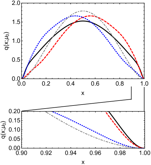
Figure 1: The pion and kaon PDF at $\mu_{0}=520$ MeV. The solid black line depict $u^{\pi}(x,\mu_{0})$ from our calculation, with blue dotted curve for $u^{K}(x,\mu_{0})$ and red dashed curve for $\bar{s}^{K}(x,\mu_{0})$. The gray dot-dashed curve is obtained with algebraic model in Chang et al. (2014). The lower plot zooms into the large $x$ region of upper plot.

Let’s first look at the pion $u^{\pi}(x;\mu_{0})$. The distribution is symmetric with respect to $x=1/2$, in line with the $u-d$ isospin symmetry. In this case, the quark and antiquark each carries half of the meson’s light front momentum automatically, i.e., $\langle x\rangle^{\pi}_{u}=0.5$. Note that the quark number sum rule has been implemented $\langle x^{0}\rangle^{\pi}_{u}=1$ as normalization condition. If we take only the handbag diagram, then $\langle x^{0}\rangle^{\pi}_{u}$ continues to be one, model independently Chang et al. (2014), but $\langle x\rangle^{\pi}_{u}$ becomes $0.46$. The modification term proportional to $\partial_{k_{\eta}}\bar{\Gamma}$ therefore collects the 8% missing momentum fraction back to the dressed quarks. This valence picture is further confirmed in the case of kaon, i.e., $\langle x\rangle^{K}_{u}+\langle x\rangle^{K}_{\bar{s}}=1$, more specifically $u^{K}(x)=\bar{s}^{K}(1-x)$, which is the consequence of momentum conservation in terms of dressed quarks.

Another observation is that the solid curve is broader than the dot-dashed one. The latter shows the PDF computed from an algebraic model of the propagators and Bethe-Salpeter amplitudes developed in Ref.Chang et al. (2013) and adapted by the authors of Ref.Chen et al. (2016a) (see, e.g., Eq.(8) of Chen et al. (2016a)). Such algebraic models, based on simple but insightful parameterizations of $S(k)$ and $\Gamma_{\pi}(k)$ have yielded interesting results and discussions both in the meson sector (see e.g. Gao et al. (2014); Mezrag et al. (2016); Chouika et al. (2018)) and in the baryon one Mezrag et al. (2017). In the present case, the realistic quark propagator and BS amplitudes give a broader $u^{\pi}(x;\mu_{0})$ than the one obtain with the algebraic model. The broadness discrepancy can be quantified by studying the $\langle(2x-1)^{2}\rangle_{u}^{\pi}$ of the distributions $u^{\pi}(x;\mu_{0})$. The present computation of the PDF yields $\langle(2x-1)^{2}\rangle_{u}^{\pi}=0.20$ while the algebraic model of Ref.Chen et al. (2016a) gives $\langle(2x-1)^{2}\rangle_{u}^{\pi}=0.15$. The situation is similar with kaon, i.e., $\langle(2x-1)^{2}\rangle_{u}^{K}=0.176$ versus $\langle(2x-1)^{2}\rangle_{u}^{K}=0.134$ obtained with the algebraic model of Ref.Chen et al. (2016a). From our perspective, this difference traces back to a faithful representation of the DCSB effect: the $S(k)$ and $\Gamma(k;P)$ encoding realistic DCSB effect typically generate a parton distribution amplitude (PDA) which is again broader than the one coming from the algebraic model. In the present case, the DB-kernel pion generates a pion PDA $\phi(x)\approx 1.81(x(1-x))^{0.31}(1-0.12C_{2}^{0.81}(2x-1))$, which is broader than $\phi(x)=6x(1-x)$ from algebraic model Chang et al. (2013). This feature is reflected in the case of our PDF.

The underlying connection between PDA and PDF can be viewed from the perspective of pion’s leading twist light front wave function $\psi(x,\mathbb{k}_{\perp}^{2})$ Burkardt et al. (2002); Braun and Filyanov (1990). The PDA is defined as Lepage and Brodsky (1980)

$$\phi(x,\mu^{2}) =\int^{\mu^{2}}d^{2}\mathbb{k}_{\perp}\psi(x,\mathbb{k}_{\perp}^{2}),$$ (13)

while

$$q(x,\mu_{0}^{2}) \approx\int d^{2}\mathbb{k}_{\perp}|\psi(x,\mathbb{k}_{\perp}^{2})|^{2}$$ (14)

approximates the PDF at some low hadronic scale in the absence of higher Fock state Burkardt et al. (2002) and neglecting the higher twist wave function Burkardt et al. (2002); Mezrag et al. (2016). The PDA and PDF are therefore implicitly related and the broadness in $\phi(x,\mu^{2})$ would be reflected in $q(x,\mu_{0}^{2})$, as we have observed above.

Fig. 1 also shows the SU(3) flavor symmetry breaking in the kaon PDF, as $u^{K}(x)\neq\bar{s}^{K}(x)$. The heavier $s$ quark carries a larger fraction of the meson momentum, i.e., $\langle x\rangle^{K}_{\bar{s}}=0.55$, with the rest $45\%$ carried by $u$ quark. We remind that for the kaon PDA, a similar result is obtained, i.e., $\langle(2x-1)\rangle_{\phi}=0.04$ Shi et al. (2014). The 10% difference in kaon’s $s$ and $u$ quark PDF is significantly smaller than their current quark mass ratio $m_{s}/m_{u}\gtrsim 20$. Therefore the SU(3) flavor symmetry is strongly masked by the dressing effect on light quarks through DCSB.

The end point behavior of the valence PDFs is shown in the lower plot in Fig. 1. Theoretically, as $x\rightarrow 1$, one quark carries almost all the plus momentum of its parent meson and gets far off shell. Then the pQCD becomes valid and predicts the power behavior of valence PDF $\sim(1-x)^{2}$ as $x\rightarrow 1$ Ji et al. (2005). This power behavior is respected by all our curves as shown by the plot. It starts from some inflection point around $x\gtrsim 0.95$, signaling the transition from soft nonperturbative QCD dynamics to hard pQCD interactions.

We futher parameterize our PDFs with

$$q(x;\mu_{0})=30[x(1-x)]^{2}\left[1+\sum_{j=1}^{j_{m}}a_{j}C_{j}^{5/2}(2x-1)\right].$$ (15)

We find with $j_{m}=10$ the curves can well be represented by parameters in Table. 2.

Table 2: Fitting parameters in Eq. (15) for $u^{\pi}(x,\mu_{0})$ and $\bar{s}^{K}(x,\mu_{0})$.

	$a_{1}$	$a_{2}$	$a_{3}$	$a_{4}$	$a_{5}$
$\pi$	0	0.125	0	0.0463	0
K	0.137	0.0894	0.0313	0.0292	0.00671
	$a_{6}$	$a_{7}$	$a_{8}$	$a_{9}$	$a_{10}$
$\pi$	0.0181	0	0.00651	0	0.00152
K	0.00801	0.00178	0.00214	0.000728	0.000518

We then perform the NLO DGLAP evolution on valence-quark distribution $u^{\pi}_{v}(x)=u^{\pi}(x)-\bar{u}^{\pi}(x)$ using the QCDNUM package Botje (2011). The strong coupling constant is set to be the optimal value in NLO global PDF analysis $\alpha_{s}(1\textrm{GeV})=0.491$ Martin et al. (2009) and the variable flavor number scheme (VFNS) is taken. It is found that for $u_{v}^{\pi}(x,\mu_{0})$, $\mu_{0}=520$ MeV produces $\langle x\rangle_{v}^{\pi}\sim 0.24$ at $\mu_{2}=2\textrm{GeV}$, close to the $\pi N$ Drell-Yan data analysis $2\langle x\rangle_{v}^{\mu_{2}}=0.47(2)$ Sutton et al. (1992); Gluck et al. (1999) and lattice simulation $2\langle x\rangle_{v}^{\mu_{2}}=0.48(4)$ Detmold et al. (2003). The evolved valence quark distribution $u^{\pi}_{v}(x,\mu_{4})$ with $\mu_{4}=4$ GeV is plotted in Fig. 2. As it can be seen, our result generally agrees with existing data analysis. Especially it favors the result from Aicher et al. (2010) when $x\gtrsim 0.6$. In this connection, LO analysis found almost linear decrease at large x, i.e., $\sim(1-x)^{2+\beta}$ with $\beta=-0.74$ Conway et al. (1989) while NLO analysis almost halved this value, i.e., $\beta=-0.40$ Aicher et al. (2010). The authors of Aicher et al. (2010) show that the logarithmic threshold resummation brings considerable reduction at large $x$, i.e., $\beta=0.34$ and therefore agrees with pQCD prediction $\beta>0$. Since we already have $\beta=0$ at $\mu_{0}$, DGLAP evolution to higher scale further shifts the support of $u_{v}^{\pi}(x;\mu_{0})$ from larger $x$ to smaller $x$ and therefore increases the value of $\beta$.

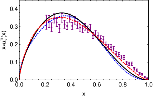
Figure 2: Our pion valence PDF NLO evolved to $\mu_{4}=4$ GeV is displayed as the black solid curve. NLO analysis of Fermilab E-615 pionic Drell-Yan data with soft-gluon resummation Aicher et al. (2010) is plotted as blue dotted curve ($\mu=4$ GeV). Without soft-gluon resummation, NLO analysis gives the red dot-dashed line ($\langle M_{\gamma}\rangle=5.2$ GeV) Wijesooriya et al. (2005). The purple filled cricles are LO analysis result ($\langle M_{\gamma}\rangle=5.2$ GeV) Conway et al. (1989).

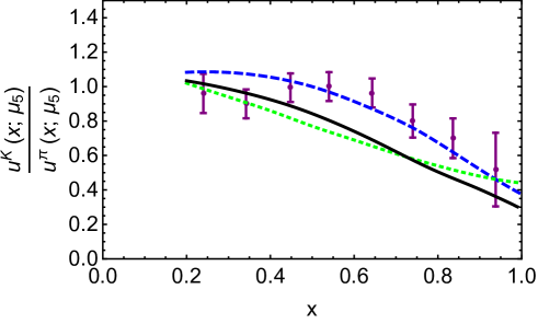
Figure 3: The ratio of $\bar{u}$ distribution function in $K^{-}$ to that of $\pi^{-}$, i.e., $\bar{u}^{K}(x;\mu_{5})/\bar{u}^{\pi}(x;\mu_{5})$ with $\mu_{5}=5.2$ GeV. The blue filled circles are experimental data from Badier et al. (1980). Our result is depicted as the black solid curve. Green dotted curve is the NJL model calculation with proper-time regularization Hutauruk et al. (2016) and blue dashed curve is from Chen et al. (2016a).

We finally depict the the ratio of $\bar{u}$ distribution function in $K^{-}$ to that of $\pi^{-}$, i.e., $\bar{u}^{K}(x;\mu_{5})/\bar{u}^{\pi}(x;\mu_{5})$ with $\mu_{5}=5.2$ GeV, in Fig. 3. Generally speaking, our result undershoots many data points in the valence region, but shows agreement at low and large $x$ region. We point out same situation occurs in the NJL model calculation with proper-time regularization (green dotted curve) Hutauruk et al. (2016), which also starts with the valence picture for mesons. The cause of the deviation at intermediate $x$ region deserves further investigation but one clue can be found in Chang et al. (2014); Chen et al. (2016a). Therein the authors point out that nonperturbatively, the pion should have more gluon content than the kaon does at certain hadronic scale $\mu_{0}^{\prime}$. By incorporating the gluon effect, they found good agreement with valence PDF data for both the pion and the kaon. Herein if we incorporate this gluon effect into our $\bar{u}^{\pi/K}(x;\mu_{0})$ and bring them to $\bar{u}^{\pi/K}(x;\mu_{0}^{\prime})$ , then the $\bar{u}^{\pi}(x;\mu_{0})$ and $\bar{u}^{K}(x;\mu_{0})$ would both shift to lower $x$ but $\bar{u}^{\pi}(x;\mu_{0})$ would shift more, since more of the quark momentum in the pion should be carried away by gluons than in the kaon. The consequence is that $\bar{u}^{K}(x;\mu_{0}^{\prime})$ would get close to $\bar{u}^{\pi}(x;\mu_{0}^{\prime})$. Note that in the large $x$ region the gluon effect is suppressed Chang et al. (2014) and the ratio changes little, i.e., $\bar{u}^{K}(x;\mu_{0}^{\prime})/\bar{u}^{\pi}(x;\mu_{0}^{\prime})|_{x\rightarrow 1}=\bar{u}^{K}(x;\mu_{0})/\bar{u}^{\pi}(x;\mu_{0})|_{x\rightarrow 1}$. In this way, the overall outcome would be raising the ratio from $\bar{u}^{K}(x;\mu_{0})/\bar{u}^{\pi}(x;\mu_{0})$ to $\bar{u}^{K}(x;\mu_{0}^{\prime})/\bar{u}^{\pi}(x;\mu_{0}^{\prime})$ in the intermediate $x$ region with the large $x$ region unchanged. After DGLAP evolution, the curve $\bar{u}^{K}(x;\mu_{5})/\bar{u}^{\pi}(x;\mu_{5})$ should inherit this remedy and get closer to the data.

IV summary

Starting with the solution of the Bethe-Salpeter equation for the pion, in a beyond rainbow-ladder truncation of QCD’s Dyson-Schwinger equations, we have computed the valence-quark PDF of pion and kaon within the modified impulse approximation. These PDFs give the purely valence picture of pion and kaon at hadronic scale, and exhibit many properties stemming from QCD. For instance, the dynamical chiral symmetry breaking generally broadens the PDFs at hadronic scale, similarly to the case of parton distribution amplitude. The $SU(3)$ flavor symmetry breaking, masked by the DCSB, causes typically $10\%$ asymmetry in the kaon’s PDFs. At large $x$, all our PDFs decreases with the power behavior $\sim(1-x)^{2}$, respecting the pQCD prediction. We then evolve these valence quark distribution functions to experimental scale. Despite good agreement with the pion valence PDF, the ratio $\bar{u}^{K}(x;\mu_{5})/\bar{u}^{\pi}(x;\mu_{5})$ generally undershoots the data. We therefore sketch a resolution to this discrepancy, based on the argument that the pion hosts more gluons than the kaon at hadronic scale Chen et al. (2016a). Nevertheless in the DSE-BSE framework, a conclusive verification of this problem calls for a nonperturbative study on the pion and kaon bound state equations incorporating $q\bar{q}g$ component.

Appendix A

In obtaining Eq. (12) from Eqs. (11), we find the following integral variable transformation useful,

$$\prod_{i=1}^{3}\int_{0}^{1}dx_{i}\prod_{j=1}^{2}\int_{-1}^{1}d\alpha_{j}=\prod_{i=1}^{5}\int_{0}^{1}da_{i}|J_{a}|+\prod_{i=1}^{5}\int_{0}^{1}db_{i}|J_{b}|.$$ (16)

$|J_{a}|$ and $|J_{b}|$ are the Jacobian determinants of the new integral variables $a_{i}$ and $b_{i}$. We introduce some auxiliary variables as

$$u =(1-\alpha_{1})/2$$ (17)

$$v =(2-x_{3}-x_{3}\alpha_{2})(1-x_{2})/2$$ (18)

$$z =ux_{1}+v(1-x_{1}),$$ (19)

then the variable transformation is

$$a_{1} =z$$ (20)

$$a_{2} =\frac{u}{z}$$ (21)

$$a_{3} =\frac{x_{1}(1-u)}{1-z}$$ (22)

$$a_{4} =\frac{x_{2}}{1-v}$$ (23)

$$a_{5} =\frac{x_{3}-(1-v/(1-x_{2}))}{v/(1-x_{2})}$$ (24)

and $b_{i}=a_{i}$ except $b_{2}=(u-z)/(1-z)$ and $b_{3}=x_{1}u/z$. In practice, this brings Eq. (11) to the form

$$\langle x^{m}\rangle=\int_{0}^{1}da_{1}a_{1}^{m}(G_{0}+G_{1}m+G_{2}m^{2}+G_{3}m^{3})$$ (25)

where $G_{i}$’s are functions of $a_{1}$ and has no dependence in $m$. To further reduce it to Eq. (12), we need to remove terms proportional to $m^{i}$ with $i>0$. We exemplify with the term $\int_{0}^{1}da_{1}a_{1}^{m}m^{2}G_{2}$. The starting point is the identity

$$\int_{0}^{1}da_{1}\frac{\textrm{d}^{2}(a_{1}^{m+2}G_{2})}{\textrm{d}a_{1}^{2}}=0.$$ (26)

The equality can be checked numerically. Fully expand the derivative in the integrand and one gets

$$\int_{0}^{1}da_{1}a_{1}^{m}m^{2}G_{2} =\int_{0}^{1}da_{1}a_{1}^{m}[-m(3G_{2}+2a_{1}G_{2}^{\prime})$$

$$-(2G_{2}+4a_{1}G_{2}^{\prime}+a_{1}^{2}G_{2}^{\prime\prime})].$$ (27)

The term proportional to $m^{2}$ is reduced to terms of $m^{1}$ and $m^{0}$. Therefore in practice we start from the $m^{3}$ term and employing similar procedures iteratively until all the terms proportional to $m^{i}$ with $i>0$ are removed, leaving only Eq. (12).