Conditional Sparse $\ell_{p}$-norm Regression With Optimal Probability

Abstract

We consider the following conditional linear regression problem: the task is to identify both (i) a $k$-DNF condition $c$ and (ii) a linear rule $f$ such that the probability of $c$ is (approximately) at least some given bound $\mu$, and $f$ minimizes the $\ell_{p}$ loss of predicting the target $z$ in the distribution of examples conditioned on $c$. Thus, the task is to identify a portion of the distribution on which a linear rule can provide a good fit. Algorithms for this task are useful in cases where simple, learnable rules only accurately model portions of the distribution. The prior state-of-the-art for such algorithms could only guarantee finding a condition of probability $\Omega(\mu/n^{k})$ when a condition of probability $\mu$ exists, and achieved an $O(n^{k})$-approximation to the target loss, where $n$ is the number of Boolean attributes. Here, we give efficient algorithms for solving this task with a condition $c$ that nearly matches the probability of the ideal condition, while also improving the approximation to the target loss. We also give an algorithm for finding a $k$-DNF reference class for prediction at a given query point, that obtains a sparse regression fit that has loss within $O(n^{k})$ of optimal among all sparse regression parameters and sufficiently large $k$-DNF reference classes containing the query point.

1 Introduction

In areas such as advertising, it is common to break a population into segments, on account of a belief that the population as a whole is heterogeneous, and thus better modeled as separate subpopulations. A natural question is how we can identify such subpopulations. A related question arises in personalized medicine. Namely, we need existing cases to apply data-driven methods, but how can we identify cases that should be grouped together in order to obtain more accurate models?

In this work, we consider a problem of this sort recently formalized by Juba 2017: we are given a data set where each example has both a real-valued vector together with a Boolean-valued vector associated with it. Let $\vec{Y}$ denote the real-valued vector for some example, and let $\vec{X}$ denote the vector of Boolean attributes. We are also given some target prediction $Z$ of interest, and we wish to identify a $k$-DNF $c$ such that $c(\vec{X})$ specifies a subpopulation on which we can find a linear predictor for $Z$, $\langle\vec{a},\vec{Y}\rangle$, that achieves small loss. In particular, it may be that neither $\vec{a}$, nor any other linear predictor achieves small loss over the entire data distribution, and we simply wish to find the subset of the distribution, determined by our $k$-DNF $c$ evaluated on the Boolean attributes of our data, on which accurate regression is possible. We refer to this subset of the distribution as a "segment".

Juba proposed two algorithms for different families of loss functions, one for the sup norm (that only applies to $O(1)$-sparse regression) and one for the usual $\ell_{p}$ norms. But, the algorithm for the $\ell_{p}$ norm has a major weakness, namely that it can only promise to identify a condition $c^{\prime}(\vec{X})$ that has a probability polynomially smaller than optimal. This is especially problematic if the segment had relatively small probability to begin with: it may be that there is no such condition with enough examples in the data for adequate generalization. By contrast, the algorithm for the sup norm recovers a condition $c^{\prime}$ with probability essentially the same as the optimal condition, but of course the sup norm is an undesirable norm to use for regression, as it is maximally sensitive to outliers. In general, $\ell_{p}$ regression is more tolerant to outliers as $p$ decreases, and the sup norm is roughly “$p=\infty$.”

In this work, in Theorem 10, we show how to give an algorithm for $O(1)$-sparse $\ell_{p}$ regression with a two-fold improvement over the previous $\ell_{p}$ regression algorithm (mentioned above) when the coefficient vector is sparse:

1. The new algorithm recovers a condition $c^{\prime}$ with probability essentially matching the optimal condition.

2. We also obtain a smaller blow-up of the loss relative to the optimal regression parameters $\vec{a}$ and optimal condition $c$, reducing the degree of this polynomial factor.

More concretely, Juba’s previous algorithm identifies $k$-DNF conditions, as does ours. This algorithm only identified a condition of probability $\Omega(\mu/n^{k})$ when a condition with probability $\mu$ exists, and only achieved loss bounded by $O(\epsilon n^{k})$ when it is possible to achieve loss $\epsilon$. We improve the probability of the condition to $(1-\eta)\mu$ for any desired $\eta>0$, and also reduce the bound on the loss to $\tilde{O}(\epsilon n^{k/2})$, or further to $\tilde{O}(\epsilon g\log\log(n^{k}))$ if the condition has only $g$ “terms” (ANDs of literals), in Corollary 12. This latter algorithm furthermore features a smaller sample complexity, that only depends logarithmically on the number $n$ of Boolean attributes. We include a synthetic data experiment demonstrating that the latter algorithm can successfully recover more terms of a planted solution than Juba’s sup norm algorithm.

We also give an algorithm for the closely related reference class regression problem in Theorem 14. In this problem, we are given a query point $\vec{x}^{*}$ (along with values for the real attributes $\vec{y}^{*}$), and we wish to estimate the corresponding $z^{*}$. In order to compute this estimate for a single point, we find some $k$-DNF $c^{\prime}$ such that $c^{\prime}(\vec{x}^{*})=1$ so $\vec{x}^{*}$ is in the support of the distribution conditioned on $c^{\prime}(\vec{X})$, and such that there are (sparse) regression parameters $\vec{a}^{\prime}$ for $c^{\prime}$ that (nearly) match the optimal loss for sparse regression under any condition $c$ with $c(\vec{x}^{*})=1$. In this case, the condition $c^{\prime}$ is a reference class containing $\vec{x}^{*}$, obtaining the tightest possible fit among $k$-DNF classes containing $\vec{x}^{*}$. We think of this as describing a collection of “similar cases” for use in estimating the target value $z^{*}$ from the attributes $\vec{y}^{*}$. For this problem, we guarantee that we find a condition $c^{\prime}$ and sparse regression parameters $\vec{a}^{\prime}$ that achieve loss within $O(n^{k})$ of optimal.

Our algorithms are based on sparsifiers for linear systems, for example as obtained for the $\ell_{2}$ norm by Batson et al. 2012, and as obtained for non-Euclidean $\ell_{p}$ norms by Cohen and Peng 2015 based on Lewis weights (Lewis, 1978). The strategy is similar to Juba’s sup norm algorithm: there, by enumerating the vertices of the polytopes obtained on various subsets of the data, he is able to obtain a list of all possible candidates for the optimal estimates of the sup-norm regression coefficients. Here, we can similarly obtain such a list of estimates for the $\ell_{p}$ norms by enumerating the possible sparsified linear systems. Sparsifiers are often used to accelerate algorithms, e.g., to run in time in terms of the number of nonzero entries rather than the size of the overall input, though here we use that the size of a sparsified representation is small in a rather different way. Namely, the small representation allows for a feasible enumeration of possible candidates for the regression coefficients.

We note that this means that we also obtain an algorithm for $O(1)$-sparse $\ell_{p}$-norm regression in the list-learning model (Balcan et al., 2008; Charikar et al., 2017). Although Charikar et al. in particular are able to solve a large family of problems in the list-learning model, they observe that their technique can only obtain trivial estimates for regression problems. We show that once we have such a list, algorithms for the conditional distribution search problem (Juba, 2016; Zhang et al., 2017; Juba et al., 2018) can be generically used to extract a description of a good event $c$ for the given candidate linear rule. Similar algorithms can also then be used to find a good reference class.

1.1 Relationship to other work

The conditional linear regression problem is most closely related to the problem of prediction with a “reject” option. In this model, a prediction algorithm has the option to abstain from making a prediction. In particular, El-Yaniv and Weiner 2012 considered linear regression in such a model. However, like most of the work in this area, their approach is based on scoring the “confidence” of a prediction function, and only making a prediction when the confidence is sufficiently high. This does not necessarily yield a nice description of the region in which the predictor will actually make predictions. On the other hand, Cortes et al. 2016 consider an alternative variant of learning with rejection that does obtain such nice descriptions; but, in their model, they assume that abstention comes at a fixed, known cost, and they simply optimize the overall loss when their space of possible prediction values includes this fixed-cost “abstain” option. By contrast, we can explicitly consider various rates of coverage or loss.

Our work is also related to the field of robust statistics (Huber, 1981; Rousseeuw and Leroy, 1987): in this area, one seeks to mitigate the effect of outliers. That is, roughly, we suppose that a small fraction of the data has been corrupted, and we wish for our models and inferences to be relatively unaffected by this corrupted data. The difference between robust statistics and the conditional regression problem is that in conditional regression we are willing to ignore most of the data. We only wish to find a small fraction, described by some rule, on which we can obtain a good regression fit.

Another work that similarly focuses on learning for small subsets of the data is the the work by Charikar et al. 2017 in the list-learning model of Balcan et al. 2008. In that work, one seeks to find a setting of some parameters that (nearly) minimizes a given loss function on an unknown small subset of the data. Since it is generally impossible to produce a single set of parameters to solve this task – many different small subsets could have different choices of optimal parameters – the objective is to produce a small list of parameters that contains a near-optimal solution for the unknown subset somewhere in it. As we mentioned above, our approach actually gives a list-learning algorithm for $O(1)$-sparse $\ell_{p}$ regression; but, we show furthermore how to identify a conditional distribution such that some regression fit in the list obtains a good fit, thus also solving the conditional linear regression task. Indeed, in general, we find that algorithms for solving the list-learning task for regression yield algorithms for conditional linear regression. The actual technique of Charikar et al. does not solve our problem since their approximation guarantee essentially always admits the zero vector as a valid approximation. Thus, they also do not obtain an algorithm for list-learning (sparse) regression either.

Another task similar to list-learning of linear regression is the problem of finding dense linear relationships, as solved by RANSAC (Fischler and Bolles, 1981). But, these techniques only work in constant dimension. By contrast, although we are seeking sparse regression rules, this is a sparse fit in high dimension. As with list-learning, in contrast to the conditional regression problem, such algorithms do not provide a description of the points fitting the dense linear relationship.

Finally, yet another task similar to list-learning for regression is fitting linear mixed models (McCulloch and Searle, 2001; Jiang, 2007). In this approach, one seeks to explain all (or almost all) of the data as a mixture of several linear rules. The guarantee here is incomparable to ours: in contrast to list-learning, the linear mixed model simply needs a list of linear rules that accounts for nearly all of the data; it does not need to find a list that accounts for all possible sufficiently large subsets of the data. So, there is no guarantee that any of the mixture components represent an approximation to the regression parameters corresponding to an event of interest. On the other hand, in linear mixed models, one does not need to give any description at all of which points should lie in which of the mixture components. In applications, one usually assigns points to the linear rule that gives it the smallest residual, but this may be less useful for predicting the values for new points.

2 Preliminaries

We now formally define the problems we consider in this work, and recall the relevant background.

2.1 The conditional regression and distribution search tasks

Formally, we focus on the following task:

Definition 1 (Conditional $\ell_{p}$-norm Regression)

Conditional $\ell_{p}$-norm linear regression is the following task. Suppose we are given access to i.i.d. examples drawn from a joint distribution over $(\vec{X},\vec{Y},Z)\in\{0,1\}^{n}\times\{\vec{y}\in\mathbb{R}^{d}:\|y\|_{2}\leq b\}\times[-b,b]$ such that for some $k$-DNF $c^{*}$ and some coefficient vector $\vec{a}^{*}\in\mathbb{R}^{d}$ with $\|\vec{a}^{*}\|_{2}\leq b$, $\mathbb{E}[|\langle\vec{a}^{*},\vec{Y}\rangle-Z|^{p}|c^{*}(\vec{X})]\leq\epsilon$ and $\Pr[c^{*}(\vec{X})]\geq(1+\eta)\mu$ for some given $b>0$, $\epsilon>0$, $\eta>0$, and $\mu>0$. Then we wish to find $\hat{c}$ and $\hat{\vec{a}}$ such that $\mathbb{E}[|\langle\hat{\vec{a}},\vec{Y}\rangle-Z|^{p}|\hat{c}(\vec{X})]^{1/p}\leq\alpha\epsilon$ and $\Pr[\hat{c}(\vec{X})]\geq(1-\eta)\mu$ for an approximation factor function $\alpha$.

If $\vec{a}^{*}$ has at most $s$ nonzero components, and we require $\hat{\vec{a}}$ likewise has at most $s$ nonzero components, then this is the conditional $s$-sparse $\ell_{p}$-norm regression task.

As stressed by Juba 2017, the restriction to $k$-DNF conditions is not arbitrary. If we could identify conditions that capture arbitrary conjunctions, even for one-dimensional regression, this would yield PAC-learning algorithms for general DNFs. In addition to this being an unexpected breakthrough, recent work by Daniely and Shalev-Shwartz 2016 shows that such algorithms would imply new algorithms for random $k$-SAT, falsifying a slight strengthening of Feige’s hypothesis (Feige, 2002). We thus regard it as unlikely that any algorithm can hope to find conditions of this kind. Of the classes of Boolean functions that do not contain arbitrary conjunctions, $k$-DNFs are the most natural large class, and hence are the focus for this model.

The difficulty of the problem lies in the fact that initially we are given neither the condition nor the linear predictor. Naturally, if we are told what the relevant subset is, we can just use standard methods for linear regression to obtain the linear predictor; conversely, if we are given the linear predictor, then we can use algorithms for the conditional distribution search (learning abduction) task (introduced by Juba 2016, recalled below) to identify a condition on which the linear predictor has small error. Our final algorithm actually uses this connection, by considering a list of candidates for the linear predictors to use for labeling the data, and choosing the linear predictor that yields a condition that selects a large subset. In particular, we will use algorithms for the following weighted variant of the conditional distribution search task:

Definition 2 (Conditional Distribution Search)

Weighted conditional distribution search is the following problem. Suppose we are given access to examples drawn i.i.d. from a distribution over $(\vec{X},W)\in\{0,1\}^{n}\times[0,b]$ such that there exists a $k$-DNF condition $c^{*}$ with $\Pr[c^{*}(\vec{X})]\geq(1+\eta)\mu$ and $\mathbb{E}[W|c^{*}(\vec{X})]\leq\epsilon$ for some given parameters $\eta,\mu,b,\epsilon>0$. Then, find a $k$-DNF $\hat{c}$ such that $\Pr[\hat{c}(\vec{X})]\geq(1-\eta)\mu$ and $\mathbb{E}[W|\hat{c}(\vec{X})]<\alpha\cdot\epsilon$ for some approximation factor function $\alpha$ (or INFEASIBLE if no such $c^{*}$ exists).

This task is closely related to agnostic conditional distribution search, which is the special case where the weights only take values $0$ or $1$. The current state of the art for agnostic conditional distribution search is an algorithm given by Zhang et al. 2017, achieving an $\tilde{O}(\sqrt{n^{k}})$-approximation to the optimal error. That work built on an earlier algorithm due to Peleg 2007. Peleg’s work already showed how to extend his original algorithm to a weighted variant of the problem, and we observe that an analogous modification of the algorithm used by Zhang et al. will obtain an algorithm for the more general weighted conditional distribution search problem we are considering here:

Theorem 3 (Peleg 2007, Zhang et al. 2017)

There is a polynomial-time algorithm for weighted conditional distribution search achieving an $\tilde{O}(n^{k/2}(\log b+\log 1/\eta+\log\log 1/\delta))$-approximation with probability $1-\delta$ given $m=\Theta\left(\frac{b^{3}}{\mu\epsilon\eta^{2}}(n^{k}+\log\frac{1}{\delta})\right)\text{ examples.}$

We note that it is possible to obtain much stronger guarantees when we are seeking a small formula. Juba et al. 2018 present an algorithm that, when there is a $k$-DNF with $g$ terms achieving error $\epsilon$, uses only $m=\tilde{O}(\frac{gk}{\mu\epsilon\eta^{2}}\log\frac{n}{\delta})$ examples and obtains a $k$-DNF with probability at least $(1-\eta)\mu$ and error $\tilde{O}(\epsilon g\log m)$. Although this is stated for the unweighted case (i.e., $\epsilon$ is a probability), it is easy to verify that since our loss is nonnegative and bounded, by rescaling the losses to lie in $[0,1]$, we can obtain an analogous guarantee for the weighted case:

Theorem 4 (Juba et al. 2018)

There is a polynomial-time algorithm for weighted conditional distribution search when the condition has $g$ terms using $m=\tilde{O}(\frac{bgk}{\mu\epsilon\eta^{2}}\log\frac{n}{\delta})$ examples achieving an $\tilde{O}(g\log m)$-approximation using a $k$-DNF with $\tilde{O}(g\log m)$ terms with probability $1-\delta$.

2.2 Reference class regression

Using a similar approach, we will also solve a related problem, selecting a best $k$-DNF “reference class” for regression. In this task, we are not merely seeking some $k$-DNF event of probability $\mu$ on which the conditional loss is small. Rather, we are given some specific observed Boolean attribute values $\vec{x}^{*}$, and we wish to find a $k$-DNF condition $c$ that is satisfied by $\vec{x}^{*}$ solving the previous task. That is, $c$ should have probability at least $\mu$ and our sparse regression fit has small conditional loss, conditioned on $c$. Naturally, the motivation here is that we have some specific point $(\vec{x}^{*},\vec{y}^{*})$ for which we are seeking to predict $z^{*}$, and so we are looking for a “reference class” $c$ such that we can get the tightest possible regression estimate of $z^{*}$ from $\vec{y}^{*}$; to do so, we need to take $\mu$ large enough that we have enough data to get a high-confidence estimate, and we need $\vec{x}^{*}$ to lie in the support of the conditional distribution for which we are computing this estimate.

Definition 5 (Reference Class $\ell_{p}$-Regression)

Reference class $\ell_{p}$-norm regression is the following task. We are given a query point $\vec{x}^{*}\in\{0,1\}^{n}$, target density $\mu\in(0,1)$, ideal loss bound $\epsilon_{0}>0$ approximation parameter $\eta>0$, confidence parameter $\delta>0$, and access to i.i.d. examples drawn from a joint distribution over $(\vec{X},\vec{Y},Z)\in\{0,1\}^{n}\times\{\vec{y}\in\mathbb{R}^{d}:\|\vec{y}\|_{2}\leq b\}\times[-b,b]$. We wish to find $\hat{\vec{a}}\in\mathbb{R}^{d}$ with $\|\hat{\vec{a}}\|_{2}\leq b$ and a reference class $k$-DNF $\hat{c}$ such that with probability $1-\delta$, (i) $\hat{c}(\vec{x}^{*})=1$, (ii) $\Pr[\hat{c}(\vec{X})]\geq(1-\eta)\mu$, and (iii) for a fixed approximation factor $\alpha>1$, $\mathbb{E}[|\langle\hat{\vec{a}},\vec{Y}\rangle-Z|^{p}|\hat{c}(\vec{X})]^{1/p}\leq\alpha\max\{\epsilon^{*},\epsilon_{0}\}$ where $\epsilon^{*}$ is the optimal $\ell_{p}$ loss $\mathbb{E}[|\langle\vec{a}^{*},\vec{Y}\rangle-Z|^{p}|c^{*}(\vec{X})]^{1/p}$ over $\vec{a}^{*}\in\mathbb{R}^{d}$ of $\|\vec{a}^{*}\|_{2}\leq b$ and $k$-DNFs $c^{*}$ such that $c^{*}(\vec{x}^{*})=1$ and $\Pr[c^{*}(\vec{X})]\geq\mu$. If we also require both $\hat{\vec{a}}$ and $\vec{a}^{*}$ to have at most $s$ nonzero components, then this is the reference class $s$-sparse $\ell_{p}$-norm regression task.

The selection and use of such reference classes for estimation goes back to work by Reichenbach 1949. Various refinements of this approach were proposed by Kyburg 1974 and Pollock 1990, e.g., to choose the estimate provided by the highest-accuracy reference class that is consistent with the most specific reference class containing the point of interest $\vec{x}^{*}$. Our approach is not compatible with these proposals, as they essentially disallow the use of the kind of disjunctive classes that are our exclusive focus. Along the lines we noted earlier, it is unlikely that there exist efficient algorithms for selecting reference classes that capture arbitrary conjunctions, so $k$-DNFs are essentially the most expressive class for which we can hope to solve this task. Bacchus et al. 1996 give a nice discussion of other unintended shortcomings of disallowing disjunctions. A concrete example discussed by Bacchus et al. is the genetic disease Tay-Sachs. Tay-Sachs only occurs in two very specific, distinct populations: Eastern European Jews and French Canadians. Thus, a study of Tay-Sachs should consider a reference class at least partially defined by a disjunction over membership in these two populations.

2.3 $\ell_{p}$ sparsification

Our approach is based on techniques for extracting low-dimensional sketches of small subspaces in high dimensions. The usual $\ell_{2}$ norm uses much simpler underlying techniques, and we describe it first. The extension to $\ell_{p}$ norms for $p\neq 2$ is obtained via Lewis weights (Lewis, 1978).

2.3.1 Euclidean sparsifiers

The kind of sketches we need originate in the work of Batson et al. 2012. Specifically, it will be convenient to start from the following variant due to Boutsidis et al. 2014:

Lemma 6 (BSS weights (Boutsidis et al., 2014))

Let $[u]\in\mathbb{R}^{d\times t}$ ($t<d$) be the matrix with rows $\vec{u}_{1},\ldots,\vec{u}_{d}$ such that $\sum_{i=1}^{d}u_{i}u_{i}^{\top}=I_{t}$. Then given an integer $r\in(t,d]$, there exist $s_{1},\ldots,s_{d}\geq 0$ such that at most $r$ of the $s_{i}$ are nonzero and for the $d\times r$ matrix $[s]$ with $i$th column $\sqrt{s_{i}}\vec{e}_{i}$,

$$\lambda_{t}([u]^{\top}[s][s]^{\top}[u])\geq(1-\sqrt{t/r})^{2}\text{ and }\lambda_{1}([u]^{\top}[s][s]^{\top}[u])\leq(1+\sqrt{t/r})^{2}$$

where $\lambda_{j}$ denotes the $j$th largest eigenvalue.

In particular, taking $r=t/\gamma^{2}$ for some $\gamma\in(0,1)$, we obtain that for the $[s]$ guaranteed to exist by Lemma 6, $\|[s]^{\top}[u]\vec{v}\|_{2}^{2}=([s]^{\top}[u]\vec{v})^{\top}([s]^{\top}[u]\vec{v})$ for any $\vec{v}$, and hence by Lemma 6, $(1-\gamma)\|\vec{v}\|_{2}\leq\|[s][u]\vec{v}\|_{2}\leq(1+\gamma)\|\vec{v}\|_{2}.$ Furthermore, we can bound the magnitude of the entries of $[s]$ for orthonormal $[u]$ as follows:

Lemma 7

Suppose the rows of $[u]$ are orthonormal. Then the matrix $[s]$ obtained by Lemma 6 has entries of magnitude at most $(1+\sqrt{t/r})\sqrt{d}$.

Proof:   Observe that since the each $i$th row of $[u]$ has unit norm, it must have an entry $u_{i,j^{*}}$ that is at least $1/\sqrt{d}$ in magnitude. By the above argument,

$$\|[s]^{\top}[u]\vec{e}_{j^{*}}\|_{2}^{2}\leq(1+\sqrt{t/r})^{2}\|\vec{e}_{j^{*}}\|_{2}^{2}=(1+\sqrt{t/r})^{2}$$

where notice in particular, the $i$th row of $[s]^{\top}$ contributes at least $(\sqrt{s_{i}}u_{i,j^{*}})^{2}\geq s_{i}/d$ to the norm. Thus, $s_{i}\leq(1+\sqrt{t/r})^{2}d$.     

2.3.2 Sparsifiers for non-Euclidean norms

It is possible to obtain an analogue of the BSS weights for $p\neq 2$ using techniques based on Lewis weights (Lewis, 1978). Lewis weights are a general way to reduce problems involving $\ell_{p}$ norms to analogous $\ell_{2}$ computations. Cohen and Peng 2015 applied this to sparsification to obtain the following family of sparsifiers:

Theorem 8 ($\ell_{p}$ weights (Cohen and Peng, 2015))

Given a $d\times t$ matrix $[u]$ there exists a set of $r(p,t,\gamma)$ weights $s_{1},\ldots,s_{r}$ such that for the $d\times r$ matrix $[s]$ which has as its $i$th column $s_{i}\vec{e}_{i}$,

$$(1-\gamma)\|[u]\vec{v}\|_{p}\leq\|[s]^{\top}[u]\vec{v}\|_{p}\leq(1+\gamma)\|[u]\vec{v}\|_{p}$$

where $r(p,t,\gamma)$ is asymptotically bounded as in Table 1.

Table 1: Dimension required for $(1\pm\gamma)$-approximate $\ell_{p}$ sparsification of $t$-dimensional subspaces. $p=2$ uses BSS weights.

$p$	Required dimension $r$
$p=1$	$\frac{t\log t}{\gamma^{2}}$
$1<p<2$	$\frac{1}{\gamma^{2}}t\log(t/\gamma)\log^{2}\log(t/\gamma)$
$p=2$	$t/\gamma^{2}$
$p>2$	$\frac{\log 1/\gamma}{\gamma^{5}}t^{p/2}\log t$

Cohen and Peng also show how to construct the sparsifiers for a given matrix efficiently, but we won’t be able to make use of this, since we will be searching for the sparsifier for an unknown subset of the rows.

We furthermore obtain an analogue of Lemma 7 for the $\ell_{p}$ weights, using essentially the same argument:

Lemma 9

Suppose the rows of $[u]$ are orthonormal. Then the matrix $[s]$ obtained by Theorem 8 has entries of magnitude at most $(1+\gamma)\sqrt{d}$.

3 The weighting algorithms for conditional and reference class regression

The results from sparsification of linear systems tell us that we can estimate the loss on the subset of the data selected by the unknown condition by computing the loss on an appropriate “sketch,” a weighted average of the losses on a small subset of the data. The dimensions in Table 1 give the size of these sparsified systems, i.e., the number of examples from the unknown subset we need to use to estimate the loss over the whole subset. The key point is that since the predictors are sparse, the dimension is small; and, since we are willing to accept a constant-factor approximation to the loss, a small number of points suffice. Therefore, it is feasible to enumerate these small tuples of points to obtain a list of candidate sets of points for use in the sketch. We also need to enumerate the weights for these points, but since we have also argued that the weights are bounded and we are (again) willing to tolerate a constant-factor approximation to the overall expression, there is also a small list of possible approximate weights for the points. The collection of points, together with the weights, gives a candidate for what might be an appropriate sketch for the empirical loss on the unknown subset. We can use each such candidate approximation for the loss to recover a candidate for the linear predictor. Thus, we obtain a list of candidate linear predictors that we can use to label our data as described above. More precisely, our algorithm is as shown in Algorithm 1. In the following, let $\Pi_{d_{1},\ldots,d_{s}}$ denote the projection to coordinates $d_{1},d_{2},\ldots,d_{s}$.

input : Examples $(\vec{x}^{(1)},\vec{y}^{(1)},z^{(1)}),\ldots,(\vec{x}^{(m)},\vec{y}^{(m)},z^{(m)})$, target loss bound $\epsilon$ and fraction $\mu$.

output : A $k$-DNF over $x_{1},\ldots,x_{n}$ and linear predictor over $y_{1},\ldots,y_{d}$, or INFEASIBLE if none exist.

subroutines : WtCond takes as inputs examples $(\vec{x}^{(1)},\ldots,\vec{x}^{(m)})$, nonnegative weights $(w^{(1)},\ldots,w^{(m)})$, and a bound $\mu$, and returns a $k$-DNF $\hat{c}$ over $x_{1},\ldots,x_{n}$ solving the weighted conditional distribution search task.

begin

       Let $m_{0}=\lceil\frac{1}{\mu}(\frac{b^{2p}}{\gamma^{2p}\epsilon^{2p}}(2pb+\sqrt{2\ln(12/\delta)})^{2}+\ln\frac{3}{\delta})\rceil$, $r$ is as given in Table 1.

       forall $(d_{1},\ldots,d_{s})\in{[d]\choose s}$, $(q_{1},\ldots,q_{r})\in\{-\lceil\frac{1}{\gamma}(\ln r-\frac{1}{p}\ln\gamma)\rceil,\ldots,0,\ldots,\lceil\ln(s+1)/2\gamma\rceil\}$ and $(j_{1},\ldots,j_{r})\in{[m]\choose r}$ do

             Let $\vec{a}$ be a solution to the following convex optimization problem: minimize $\sum_{\ell=1}^{r}((1+\gamma)^{q_{\ell}}(\langle\vec{a},\Pi_{d_{1},\ldots,d_{s}}\vec{y}^{(j_{\ell})}\rangle-z^{(j_{\ell})})^{p}$ subject to $\|\vec{a}\|_{p}\leq b$.

            Put $c\leftarrow$ the output of WtCond on $(\vec{x}^{(1)},\ldots,\vec{x}^{(m)})$ with the weights $w^{(i)}=|\langle\vec{a},\Pi_{d_{1},\ldots,d_{s}}\vec{y}^{(i)}\rangle-z^{(i)}|^{p}$ and bound $\mu$.

             if WtCond did not return INFEASIBLE and $\hat{\mathbb{E}}[(\langle\vec{a},\Pi_{d_{1},\ldots,d_{s}}\vec{Y}\rangle-Z)^{p}|c(\vec{X})]^{1/p}\leq\alpha\epsilon$ then  return $\vec{a}$ and $c$.

            

       end forall

      return INFEASIBLE.

end

Algorithm 1 Weighted Sparse Regression

Theorem 10 (Conditional sparse $\ell_{p}$-norm regression)

For any constant $s$ and $\gamma>0$, $r$ as given in Table 1 for $t=(s+1)$, and $m=\Theta\left(\frac{((1+\gamma)b)^{3}}{\mu\epsilon\eta^{2}}(n^{k}+s\log d+r\log\frac{m_{0}\log(\gamma^{1/p}s/r)}{\gamma}+\log\frac{1}{\delta})+m_{0}\right)$ examples, Algorithm 1 runs in polynomial time and solves the conditional $s$-sparse $\ell_{p}$ regression task with $\alpha=\tilde{O}((1+\gamma)\sqrt{n^{k}}(\log b+\log\frac{1}{\eta}+\log\log\frac{1}{\delta})\epsilon)$.

In our proof of this theorem, we will find it convenient to use the Rademacher generalization bounds for linear predictors (note that $x\mapsto|x|^{p}$ is $pb^{p-1}$-Lipschitz on $[-b,b]$):

Theorem 11 (Bartlett and Mendelson 2002, Kakade et al. 2009)

For $b>0$, $p\geq 1$, random variables $(\vec{Y},Z)$ distributed over $\{\vec{y}\in\mathbb{R}^{d}:\|y\|_{2}\leq b\}\times[b,b]$, and any $\delta\in(0,1)$, let $L_{p}(\vec{a})$ denote $\mathbb{E}[|\langle\vec{a},\vec{Y}\rangle-Z|^{p}]$, and for an an i.i.d. sample of size $m$ let $\hat{L}_{p}(\vec{a})$ be the empirical loss $\frac{1}{m}\sum_{j=1}^{m}|\langle\vec{a},\vec{y}^{(j)}\rangle-z^{(j)}|^{p}.$ We then have that with probability $1-\delta$ for all $\vec{a}$ with $\|a\|_{2}\leq b$,

$$|L_{p}(\vec{a})-\hat{L}_{p}(\vec{a})|\leq\frac{2pb^{p+1}}{\sqrt{m}}+b^{p}\sqrt{\frac{2\ln(4/\delta)}{m}}.$$

Note that although this bound is stated in terms of the $\ell_{2}$ norm of the attribute and parameter vectors $\vec{y}$ and $\vec{a}$, we can obtain a bound in terms of the dimension $s$ of the sparse rule if we are given a bound $B$ on the magnitude of the entries: $b\leq\sqrt{s}B$.

Proof of Theorem 10:   Given that we are directly checking the empirical $\ell_{p}$ loss before returning $\vec{a}$ and $c$, for the quoted number of examples $m$ it is immediate by a union bound over the iterations that any $\vec{a}$ and $c$ we return are satisfactory with probability $1-\delta$. All that needs to be shown is that the algorithm will find a pair that passes this final check.

By Theorem 11, we note that it suffices to have $\frac{b^{2p}}{\gamma^{2p}\epsilon^{2p}}(2pb+\sqrt{2\ln(12/\delta)})^{2}$ examples from the distribution conditioned on the unknown $k$-DNF event $c^{*}$ to obtain that the $\ell_{p}$ loss of each candidate for $\vec{a}$ is estimated to within an additive $\gamma\epsilon$ with probability $1-\delta/3$. By Hoeffding’s inequality, therefore when we draw $m_{0}$ examples, there is a sufficiently large subset satisfying $c^{*}$ with probability $1-\delta/3$.

We let $[u]$ be an orthonormal basis for $\mathrm{span}\{(\Pi_{d_{1},\ldots,d_{s}}\vec{y}^{(j)},z^{(j)}):c^{*}(\vec{x}^{(j)})=1,j\leq m_{0}\}$ and invoke Lemma 6 for $\ell_{2}$ or Theorem 8 for $p\neq 2$. In either case, there is some set of weights $s_{1},\ldots,s_{r_{0}}$ for a subset of $r_{0}$ coordinates $j_{1},\ldots,j_{r_{0}}$ such that for any $\vec{v}$ in the column span of $[u]$, $[s]^{\top}[u]\vec{v}$ has $\ell_{p}$ norm that is a $1\pm\gamma$-approximation to the $\ell_{p}$ norm of $[u]\vec{v}$. In particular, for any $\vec{a}$, observing $\vec{v}=[y]\vec{a}-\vec{z}$ is in the column span of $[u]$ by construction, we obtain

$$(1-\gamma)\|[y]\vec{a}-\vec{z}\|_{p}\leq\|[s]^{\top}([y]\vec{a}-\vec{z})\|_{p}\leq(1+\gamma)\|[y]\vec{a}-\vec{z}\|_{p}.$$

Now, we observe that we can discard weights (and dimensions) from $s_{1},\ldots,s_{r_{0}}$ of magnitude smaller than $\gamma/r_{0}^{1/p}$, since for any unit vector $\vec{v}$, the contribution of such entries to $\|[s]^{\top}[u]\vec{v}\|_{p}^{p}$ (recalling there are at most $r_{0}$ nonzero entries) is at most $\gamma^{p}$. So we may assume the $r\leq r_{0}$ remaining weights all have magnitude at least $\gamma/r^{1/p}$. Furthermore, if we round each weight to the nearest power of $(1+\gamma)$, this only changes $\|[s]^{\top}[u]\vec{v}|_{p}^{p}$ by an additional $(1\pm\gamma)$ factor. Finally, we note that since $(\Pi_{d_{1},\ldots,d_{s}}\vec{y}^{(j)},z^{(j)})$ has dimension $s+1$, Lemmas 7 and 9 guarantee that the magnitude is also at most $(1+\gamma)\sqrt{s+1}$. Thus it indeed suffices to find the powers $(q_{1},\ldots,q_{r})$ for our $r$ examples $j_{1},\ldots,j_{r}$ such that $(1+\gamma)^{q_{\ell}}$ is within $(1+\gamma)$ of $s_{\ell}$, and the resulting set of weights will approximate the $\ell_{p}$-norm of every $\vec{v}$ in the column span to within a $1+3\gamma$-factor.

Now, when the loop in Algorithm 1 considers (i) the dimensions $d^{*}_{1},\ldots,d^{*}_{s}$ contained in the optimal $s$-sparse regression rule $\vec{a}^{*}$ (ii) the set of examples $j^{*}_{1},\ldots,j^{*}_{r}$ used for the sparse approximation for these coordinates and (iii) the appropriate weights $(1+\gamma)^{q^{*}_{1}},\ldots,(1+\gamma)^{q^{*}_{r}}$, the algorithm will obtain a vector $\vec{a}$ that achieves a $(1+3\gamma)$-approximation to the empirical $\ell_{p}$-loss of $\vec{a}^{*}$ on the same $s$ coordinates.

It then follows from Theorem 3 that with probability at least $1-\delta/3$ over the data, WtCond will in turn return to us a $k$-DNF $c$ with probability $(1-\eta)\mu$ that selects a subset of the data on which $\vec{a}$ achieves an $\alpha\epsilon=\tilde{O}((1+\gamma)\sqrt{n^{k}}(\log b+\log 1/\eta+\log\log 1/\delta)\epsilon)$ approximation to the empirical $\ell_{p}$ loss of $\vec{a}^{*}$ on $c^{*}$. This choice of $\vec{a}$ and $c$ passes the final check and is thus sufficient.     

By simply plugging in the algorithm from Theorem 4 for WtCond, we can obtain the following improvement when the desired $k$-DNF condition is small:

Corollary 12

For any constant $s$ and $\gamma>0$, $r$ as given in Table 1 for $t=(s+1)$, and $m=\Theta\left(\frac{(1+\gamma)bgk}{\mu\epsilon\eta^{2}}\left(\log\frac{n}{\delta}+s\log d+r\log\frac{m_{0}\log(\gamma^{1/p}s/r)}{\gamma}\right)+m_{0}\right)$ examples, if there is a $g$-term $k$-DNF solution to the conditional $s$-sparse $\ell_{p}$-regression task, then the modified Algorithm 1 runs in polynomial time and solves the task with a $\tilde{O}(g\log m)$-term $k$-DNF with $\alpha=\tilde{O}((1+\gamma)\epsilon g\log m)$.

Note that this guarantee is particularly strong in the case where the $k$-DNF would be small enough to be reasonably interpretable by a human user.

The extension to reference class $\ell_{p}$-norm regression proceeds by replacing the weighted condition search algorithm with a variant of the tolerant elimination algorithm from Juba 2016, given in Algorithm 2.

input : Examples $(\vec{x}^{(1)},w^{(1)}),\ldots,(\vec{x}^{(m)},w^{(m)})$, query point $\vec{x}^{*}$, minimum fraction $\mu_{0}$, minimum loss target $\epsilon_{0}$, approximation parameter $\eta$.

output : A $k$-DNF over $x_{1},\ldots,x_{n}$.

begin

       Initialize $\mu\leftarrow 1$, $\hat{c}\leftarrow\bot$, $\hat{\epsilon}\leftarrow\max_{j}w^{(j)}$

       while $\mu\geq\mu_{0}$ do

             Initialize $\epsilon\leftarrow\hat{\epsilon}$

             while $\epsilon\geq\epsilon_{0}/(1+\eta)$ do

                   Initialize $c$ to be the empty disjunction

                   forall Terms $T$ of at most $k$ literals do

                         if $\sum_{j:T(\vec{x}^{(j)})=1}w^{(j)}\leq\epsilon\mu m$ then  Add $T$ to $c$.

                        

                   end forall

                  Put $\epsilon\leftarrow\epsilon/(1+\eta)$

             end while

            if $c(\vec{x}^{*})=1$, $\sum_{j=1}^{m}c(\vec{x}^{(j)})\geq\mu m$, and $\epsilon<\hat{\epsilon}$ then  Put $\hat{c}\leftarrow c$, $\hat{\epsilon}\leftarrow\epsilon$

             Put $\mu\leftarrow\mu/(1+\eta)$

       end while

      return $\hat{c}$

end

Algorithm 2 Reference Class Search

Lemma 13

If $m\geq\Omega(\frac{b^{3}}{\eta^{2}(\epsilon_{0}+\epsilon^{*})\mu_{0}}(k\log n+\log\frac{1}{\eta\delta}+\log\log\frac{1}{\mu_{0}}+\log\log\frac{b}{\epsilon_{0}}))$ where $W\in[0,b]$, then Algorithm 2 returns a $k$-DNF $\hat{c}$ such that with probability $1-\delta$, 1. $\hat{c}(\vec{x}^{*})=1$ 2. $\Pr[\hat{c}(\vec{X})]\geq\mu_{0}/(1+\eta)$ 3. $\mathbb{E}[W|\hat{c}(\vec{X})]\leq O((1+\eta)^{4}n^{k}(\epsilon_{0}+\epsilon^{*}))$where $\epsilon^{*}$ is the minimum $\mathbb{E}[W|c^{*}(\vec{X})]$ over $k$-DNF $c^{*}$ such that $c^{*}(\vec{x}^{*})=1$ and $\Pr[c^{*}(\vec{X})]\geq(1+\eta)\mu_{0}$.

Proof:   For convenience, let $N\leq(1+\log_{1+\eta}b/\epsilon_{0})(1+\log_{1+\eta}1/\mu_{0})$ denote the total number of iterations. Consider first what happens when the loop considers the largest $\mu\leq\Pr[c^{*}(\vec{X})]/(1+\eta)$ and the smallest $\epsilon$ that is at least $(1+\eta)^{2}\epsilon^{*}$. On this iteration, for each term $T$ of $c^{*}$, we observe that $\mathbb{E}[W\cdot T(\vec{X})]\leq\epsilon^{*}\Pr[c^{*}(\vec{X})]$—indeed,

$$\mathbb{E}[W\cdot T(\vec{X})]\leq\mathbb{E}[W\cdot c^{*}(\vec{X})]\leq\epsilon^{*}\Pr[c^{*}(\vec{X})].$$

So, since $W$ is bounded by $b$, by a Chernoff bound, $\frac{1}{m}\sum_{j:T(x^{(j)})=1}w^{(j)}\leq(1+\eta)\epsilon^{*}\Pr[c^{*}(\vec{X})]$ with probability $1-\frac{\delta}{2{n\choose\leq k}N}$. Since this is in turn at most $\epsilon\mu$, $T$ will be included in $c$ on this iteration. But similarly, for $T$ not in $c$ with $\mathbb{E}[W\cdot T(\vec{X})]>(1+\eta)\mu\epsilon$, the Chernoff bound also yields that $\sum_{j:T(x^{(j)})=1}w^{(j)}\geq\epsilon\mu m$ with probability $1-\delta/2{n\choose\leq k}N$. By a union bound over all $T\in c^{*}$ and $T$ not in $c^{*}$ with such large error, we see that with probability at least $1-\delta/2N$, all of the terms of $c^{*}$ are included in $c$ and only terms with $\mathbb{E}[W\cdot T(\vec{X})]\leq(1+\eta)\mu\epsilon$ are included in $c$. So,

$$\mathbb{E}[W\cdot c(\vec{X})] \leq\sum_{T\text{ in }c}\mathbb{E}[W\cdot T(\vec{X})]$$

$$\leq O((1+\eta)n^{k}\mu\epsilon).$$

Furthermore, by yet another application of a Chernoff bound, $c^{*}$ is true of at least $\mu m$ examples with probability at least $1-\delta/2N$. Thus, with probability $1-\delta/N$, after this iteration $\hat{c}$ is set to some $k$-DNF and $\hat{\epsilon}\leq(1+\eta)^{2}\max\{\epsilon^{*},\epsilon_{0}\}$.

Now, furthermore, on every iteration, we see more generally that with probability $1-\delta/N$, only terms with $\mathbb{E}[W\cdot T(\vec{X})]\leq(1+\eta)\mu\epsilon$ are included in $c$, and $\hat{c}$ is only updated if $c(\vec{x}^{*})=1$ and $\Pr[c(\vec{X})]\geq\mu/(1+\eta)$, where $\mu\geq\mu_{0}$. Thus, for the $\hat{c}$ we return, since $\mathbb{E}[W\cdot c(\vec{X})]\leq O((1+\eta)n^{k}\mu\epsilon)$ and $\mathbb{E}[W|c(\vec{X})]=\mathbb{E}[W\cdot c(\vec{X})]/\Pr[c(\vec{X})]$, $\mathbb{E}[W|\hat{c}(\vec{X})]\leq O((1+\eta)^{2}n^{k}\hat{\epsilon})$. Thus, with probability $1-\delta$ overall, since we found above that $\hat{\epsilon}\leq(1+\eta)^{2}\max\{\epsilon^{*},\epsilon_{0}\}$, we return a $k$-DNF $\hat{c}$ as claimed.     

Now, as noted above, our algorithm for reference class regression is obtained essentially by substituting Algorithm 2 for the subroutine WtCond in Algorithm 1; the analysis, similarly, substitutes the guarantee of Lemma 13 for Theorem 3. In summary, we find:

Theorem 14 (Reference class regression)

For any constant $s$ and $\gamma>0$, $r$ as given in Table 1 for $t=(s+1)$, and $m\geq m_{0}+\Omega\left(\frac{(1+\gamma)^{3}b^{3}}{\eta^{2}(\epsilon_{0}+\epsilon^{*})\mu_{0}}\left(r\log\frac{m_{0}\log(\gamma^{1/p}s/r)}{\gamma}+\log\left(\frac{n^{k}d^{s}}{\eta\delta}\log\frac{1}{\mu_{0}}\log\frac{(1+\gamma)b}{\epsilon_{0}}\right)\right)\right)$ examples, our modified algorithm runs in polynomial time and solves the reference class $s$-sparse $\ell_{p}$ regression task with $\alpha=O((1+\gamma)(1+\eta)^{4}n^{k})$.

4 Experimental evaluation

To evaluate our algorithm’s performance in practice, we two kinds of experiments: one using synthetic data with a planted solution, and another using some standard benchmark data sets from the LIBSVM repository (Chang and Lin, 2011).

Synthetic data.

To generate the synthetic data sets, we first chose a random 2-DNF over Boolean attributes by sampling terms uniformly at random. We also fixed two out of $d$ coordinates at random and sampled parameters $\vec{a}$ from a mean $0$, variance $\sigma^{2}$ Gaussian for our target regression fit. For the actual data, we then sampled Boolean attributes $\vec{X}$ that, with 25% probability are a uniformly random satisfying assignment to the DNF and with 75% probability are a uniformly random falsifying assignment. We sampled $\vec{Y}$ from a standard Gaussian in $\mathbb{R}^{d}$. Finally, for the examples where $\vec{X}$ was a satisfying assignment, we let $Z$ be given by the linear rule $\langle\vec{a},\vec{Y}\rangle+\nu$ where $\nu$ is a mean $0$, variance $\sigma^{2}$ Gaussian; otherwise, if $\vec{X}$ was a falsifying assignment, $Z$ was set to $\nu^{*}$ where $\nu^{*}$ is a standard mean $0$, variance $1$ Gaussian. (Parameters in Table 2.) Thus, conditioned on the planted formula, there is a small-error regression fit $\vec{a}$—the expected error of $\vec{a}$ is $|\nu|$. Off of this planted formula, the expected error for the optimal prediction $z=0$ is $|\nu^{*}|=1$.

Table 2: Synthetic Data Set Properties

Size	Real Attributes ($d$)	Boolean Attributes ($\vec{X}$)	$k$-DNF Terms	Variance $\sigma^{2}$
1000	6	10	4	0.01
5000	10	50	16	0.1

For these simple data sets, we made several modifications to simplify and accelerate the algorithm. First, we simply fixed all of the weights (of the form $(1+\gamma)^{q_{i}}$) to $1$, i.e., $q_{i}=0$ for all $i$, since the leverage scores for Gaussian data (and indeed, most natural data sets) are usually small. Second, we set $m_{0}=200$ for the 1000-example data set and $m_{0}=500$ for the 5000-example data set. Third, we used the version of the algorithm for small DNFs considered in Corollary 12, that uses algorithm of Juba et al. 2018 (recalled in Theorem 4) for WtCond.

With these modifications, we ran Algorithm 1 for $\ell_{2}$ regression with $s=2$, $\gamma=1$, and $\mu=0.22$ on the 1000-example data set. The algorithm was able to identify the planted $2$-DNF together with the two components used in the regression rule in this case, and thus also we approximately identify the linear predictor. The mean squared error of the approximate predictor returned by our algorithm was $0.0149$ on the planted $2$-DNF (c.f. the ideal linear fit has variance-$0.01$ Gaussian noise added to it). However, we note that once the planted $2$-DNF has been identified, a good regression fit can be found by any number of methods. We also ran Algorithm 1 for $\ell_{2}$ regression with $s=2$, $\gamma=1$, and $\mu=0.2465$ on the 5000-example data set. The algorithm was able to identify a subset of $11$ out of the $16$ planted $k$-DNF terms, picking up about $98\%$ of the planted $k$-DNF data. The mean squared error of the approximate predictor was $0.4221$.

As a baseline, we also used the algorithm from Juba 2017 for conditional sparse sup-norm regression on our synthetic data. In order to obtain reasonable performance, we needed to make some modifications: we modified the algorithm along the lines of Algorithm 1, to only search over tuples of a random $m_{0}=200$ examples for the 1000-example data set and $m_{0}=500$ for the 5000-example data set in producing its candidate regression parameters. We also chose to take the parameters that achieved the smallest residuals under the sup norm, among those that obtained a condition satisfied by the desired fraction of the data. Again, we used $s=2$, and for the norm bound we used a threshold of $\epsilon=0.24$ for the 1000-example data set and $1.1$ for the 5000-example data set. (We considered a range of possible thresholds; when $\epsilon\approx 1.5$ on the $\sigma^{2}=0.1$ data, the sup norm algorithm starts adding terms outside the planted DNF, significantly increasing its error.) For the 1000-example data set, this algorithm was able to identify the planted $2$-DNF. However, for the 5000-example data set, it only found 10 out 16 terms of the planted $2$-DNF, picking up about $96\%$ of the planted $k$-DNF data.

Real-world benchmarks.

We also compared Algorithm 1 against selective regressors (El-Yaniv and Wiener, 2012) on some of the LIBSVM (Chang and Lin, 2011) regression data sets that were used to evaluate that work. We split each of those datasets into a training set (1/3 of the data) and test set (2/3 of the data). We generated Boolean attributes by choosing different binary splits (median, quartile) on the numerical features, excluding the target attribute. We then run our algorithm 1 on the training set to obtain a $2$-DNF. Next, we filtered both the training and test data satisfying the $2$-DNF, using the first one to train a new regression fit on the selected subset and the other as a holdout to estimate the error of this resulting regression fit. We compared this to the test error for selective regression. Risk-Coverage (RC) curves of the results are shown in Figure 1. We outperform the baseline on the Boston housing dataset, and we generally achieved lower error than the baseline for lower coverage (less than 0.5) and somewhat higher error for higher coverage for the other three data sets (Body fat, Space, and Cpusmall). Note that in addition, we obtained a $2$-DNF that describes the subpopulation on all four, which is the main advantage of our method. Since selective regression first tries to fit the entire data set, and then chooses a subset where that fixed predictor does well, it is to be expected that it may miss a small subset where a different predictor can do better, but that its freedom to abstain on a somewhat arbitrary subset may give it an advantage at high coverage.

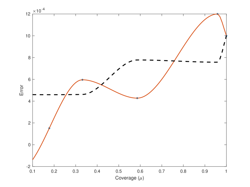
(a) Body fat

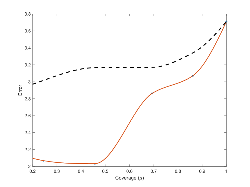
(b) Boston housing

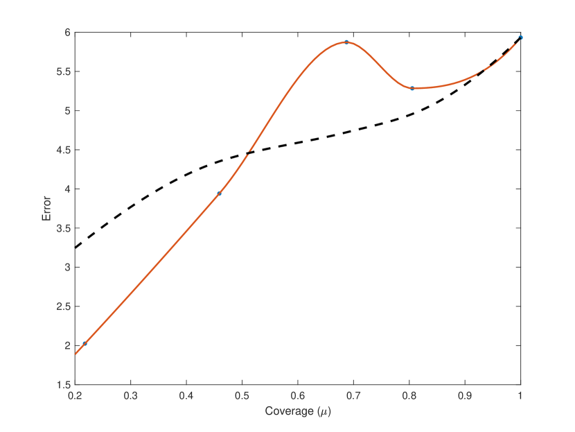
(c) Cpusmall

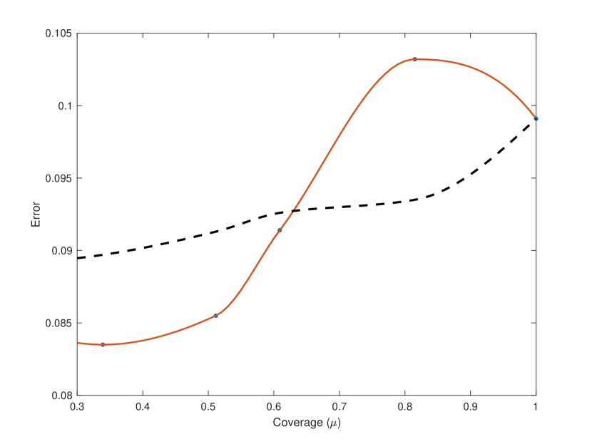
(d) Space

Figure 1: RC curves of Algorithm 1 (red line) and the baseline method (dashed line) on different regression data sets from the LIBSVM repository. The horizontal axis represents the coverage ($\mu$), while the vertical axis represents the error.

5 Directions for future work

There are several natural open problems. First, although sparsity is desirable, our exponential dependence of the running time (or list size) on the sparsity is problematic. (The sup norm regression algorithm (Juba, 2017) also suffered this deficiency.) Is it possible to avoid this? Second, our algorithm for reference class regression has an $O(n^{k})$ blow-up of the loss, as compared to $\tilde{O}(n^{k/2})$ for conditional regression. Can we achieve a similar approximation factor for reference class regression? Finally, we still do not know how close to optimal this blow-up of the loss is; in particular, we do not have any lower bounds. Note that this is a computational and not a statistical issue, since we can obtain uniform convergence over all $k$-DNF conditions.

References

- Bacchus et al. [1996] Fahiem Bacchus, Adam J. Grove, Joseph Y. Halpern, and Daphne Koller. From statistical knowledge bases to degrees of belief. Artificial Intelligence, 87:75–143, 1996.
- Balcan et al. [2008] Maria-Florina Balcan, Avrim Blum, and Santosh Vempala. A discriminative framework for clustering via similarity functions. In Proc. 40th STOC, pages 671–680, 2008.
- Bartlett and Mendelson [2002] Peter L Bartlett and Shahar Mendelson. Rademacher and gaussian complexities: Risk bounds and structural results. JMLR, 3:463–482, 2002.
- Batson et al. [2012] Joshua Batson, Daniel A Spielman, and Nikhil Srivastava. Twice-ramanujan sparsifiers. SIAM J. Comput., 41(6):1704–1721, 2012.
- Boutsidis et al. [2014] Christos Boutsidis, Petros Drineas, and Malik Magdon-Ismail. Near-optimal column-based matrix reconstruction. SIAM J. Comput., 43(2):687–717, 2014.
- Chang and Lin [2011] Chih-Chung Chang and Chih-Jen Lin. Libsvm: A library for support vector machines. ACM Trans. Intell. Syst. Technol., 2(3):27:1–27:27, May 2011. ISSN 2157-6904. doi: 10.1145/1961189.1961199. URL http://doi.acm.org/10.1145/1961189.1961199.
- Charikar et al. [2017] Moses Charikar, Jacob Steinhardt, and Gregory Valiant. Learning from untrusted data. In Proc. 49th STOC, pages 47–60, 2017.
- Cohen and Peng [2015] Michael B Cohen and Richard Peng. row sampling by lewis weights. In Proc. 47th STOC, pages 183–192, 2015.
- Cortes et al. [2016] Corinna Cortes, Giulia DeSalvo, and Mehryar Mohri. Learning with rejection. In ALT 2016, volume 9925 of LNAI, pages 67–82. 2016.
- Daniely and Shalev-Shwartz [2016] Amit Daniely and Shai Shalev-Shwartz. Complexity theoretic limtations on learning DNF’s. In Proc. 29th COLT, volume 49 of JMLR Workshops and Conference Proceedings, pages 1–16. 2016.
- El-Yaniv and Wiener [2012] Ran El-Yaniv and Yair Wiener. Pointwise tracking the optimal regression function. In Advances in Neural Information Processing Systems, pages 2042–2050, 2012.
- Feige [2002] Uriel Feige. Relations between average case complexity and approximation complexity. In Proc. 34th STOC, pages 534–543, 2002.
- Fischler and Bolles [1981] Martin A. Fischler and Robert C. Bolles. Random sample consensus: A paradigm for model fitting with applications to image analysis and automated cartography. Communications of the ACM, 24(6):381–395, 1981.
- Huber [1981] Peter J. Huber. Robust Statistics. John Wiley & Sons, New York, NY, 1981.
- Jiang [2007] Jiming Jiang. Linear and Generalized Linear Mixed Models and Their Applications. Springer, Berlin, 2007.
- Juba [2016] Brendan Juba. Learning abductive reasoning using random examples. In Proc. 30th AAAI, pages 999–1007, 2016.
- Juba [2017] Brendan Juba. Conditional sparse linear regression. In LIPIcs-Leibniz International Proceedings in Informatics, volume 67. Schloss Dagstuhl-Leibniz-Zentrum fuer Informatik, 2017. Proc. 8th ITCS.
- Juba et al. [2018] Brendan Juba, Zongyi Li, and Evan Miller. Learning abduction under partial observability. In Proc. 32nd AAAI, pages 1888–1896, 2018.
- Kakade et al. [2009] Sham M Kakade, Karthik Sridharan, and Ambuj Tewari. On the complexity of linear prediction: Risk bounds, margin bounds, and regularization. In Advances in neural information processing systems, pages 793–800, 2009.
- Kyburg [1974] Henry E. Kyburg. The Logical Foundations of Statistical Inference. Reidel, Dordrecht, 1974.
- Lewis [1978] D. Lewis. Finite dimensional subspaces of . Studia Mathematica, 63(2):207–212, 1978.
- McCulloch and Searle [2001] Charles E. McCulloch and Shayle R. Searle. Generalized, Linear, and Mixed Models. John Wiley & Sons, New York, NY, 2001.
- Peleg [2007] David Peleg. Approximation algorithms for the label-covermax and red-blue set cover problems. J. Discrete Algorithms, 5:55–64, 2007.
- Pollock [1990] John L. Pollock. Nomic Probabilities and the Foundations of Induction. Oxford University Press, Oxford, 1990.
- Reichenbach [1949] Hans Reichenbach. Theory of Probability. University of California Press, Berkeley, CA, 1949.
- Rousseeuw and Leroy [1987] Peter J. Rousseeuw and Annick M. Leroy. Robust Regression and Outlier Detection. John Wiley & Sons, New York, NY, 1987.
- Zhang et al. [2017] Mengxue Zhang, Tushar Mathew, and Brendan Juba. An improved algorithm for learning to perform exception-tolerant abduction. In Proc. 31st AAAI, pages 1257–1265, 2017.