Spectroscopic and imaging observations of small-scale reconnection events

Abstract

We present spectroscopic and imaging observations of small-scale reconnection events on the Sun. Using the Interface Region Imaging Spectrograph (IRIS) observations, one reconnection event is first detected as IRIS jets with fast bi-directional velocities in the chromosphere and transition region, which are identified as non-Gaussian broadenings with two extended wings in the line profiles of Si iv, C ii, and Mg ii k. The magnetograms under the IRIS jets from Helioseismic and Magnetic Images exhibit magnetic flux cancellation simultaneously, supporting that the IRIS jets are driven by magnetic reconnection. The Atmospheric Imaging Assembly images also show an extreme ultraviolet (EUV) brightening which is shortly after the underlying IRIS jets, i.e., in the 131 Å, 171 Å, 193 Å, 211 Å, and 94 Å channels, implying that the overlying EUV brightening in the corona is caused by the IRIS jets in the chromosphere and transition region. We also find another three reconnection events which show the same features during this IRIS observation. Our observational results suggest that the small-scale reconnection events might contribute to the coronal heating. The new result is that the process of magnetic reconnection is detected from the photosphere through chromosphere and transition region to the corona.

1 Introduction

Magnetic reconnection is a fundamental dynamical process in all magnetized astrophysical plasmas including solar atmosphere. It is thought to be the most efficient transfer of magnetic energy into plasma bulk acceleration or heating particles to the higher energy (Priest & Forbes, 2002; Mackay & Yeates, 2012). Therefore, it plays a significant role on the solar eruptions in a wide range of scales from $\sim$1000 Mm to $\sim$1 Mm, i.e., coronal mass ejections (CMEs, Lin et al., 2005), filament eruptions (Mackay et al., 2010), solar flares (Aschwanden, 2002), bright points (BPs, Priest et al., 1994), and transition-region explosive events (Innes et al., 1997). In two-dimensional (2D) reconnection model (Shibata, 1999; Priest & Forbes, 2000), it occurs at an X-point where anti-parallel magnetic field lines converge and reconnect. In the last few decades, using the high temporal and spatial resolution data, many observational evidences of magnetic reconnection on the Sun have been reported, i.e., loop-top hard X-ray source (Masuda et al., 1994), cusp-shaped post-flare loops(Tsuneta et al., 1992), reconnection inflows or outflows (Yokoyama et al., 2001; Takasao et al., 2012), magnetic null point (Zhang et al., 2012), bi-directional moving structures (Ning & Guo, 2014), and high-energetic particles (Klassen et al., 2005; Li et al., 2007), as well as the bi-directional jets with high velocity (Dere et al., 1991; Innes et al., 2015).

Using the extreme ultraviolet (EUV) and X-ray observations, Su et al. (2013) presented a process of magnetic reconnection during a solar flare, which was observed when a set of coronal loops were moving toward another set of loops and then formed an X-type structure. The X-shape geometry can also be found in two anti-parallel loops with small scale (Yang et al., 2015) or between an eruption filament and its nearby coronal loops (Li et al., 2016a). Many signatures of magnetic reconnection were observed in a spectacular eruptive flare (X8.2), such as the current sheets, reconnection inflow, hot cusp structure, and post-flare loops (Li et al., 2018; Yan et al., 2018a). These observations are based on the high-resolution imaging data (e.g., Masuda et al., 1994; Liu et al., 2010; Xue et al., 2016), such as the Reuven Ramaty High Energy Solar Spectroscopic Imager (RHESSI), the Atmospheric Imaging Assembly (AIA) and Helioseismic and Magnetic Imager (HMI) on board Solar Dynamics Observatory (SDO), and the New Vacuum Solar Telescope (NVST). On the other hand, the bi-directional plasma jets observed from the spectroscopic data usually considered as the signature of small-scale magnetic reconnection (Dere, 1994; Innes et al., 1997). They often appeared as non-Gaussian broadenings with two extended wings of spectral lines, the extended velocities could be more than 100 km s^-1 in both red and blue wings (Brueckner & Bartoe, 1983; Chae et al., 1998; Curdt et al., 2012). Using the spectroscopic observations from Solar Ultraviolet Measurements of Emitted Radiation (SUMER) and Interface Region Imaging Spectrograph (IRIS), a typical line profiles (i.e., Si iv, O iv) with non-Gaussian broadenings were found, which were produced by small-scale magnetic reconnections (Winebarger et al., 2002; Innes et al., 2015). These small-scale reconnections often appeared repetitively on the Sun (Doyle et al., 2006; Gupta & Tripathi, 2015). Besides these imaging and spectroscopic observations, the numerical results from magnetohydrodynamic (MHD) simulations (e.g., Roussev et al., 2001; Heggland et al., 2009; Ni et al., 2015) also support the fact that magnetic reconnection plays an important role in solar eruptions.

On solar surface, the temperature in the corona ($\sim$10⁶ K) is much higher than that in the photosphere ($\sim$6$\times$10³ K) and chromosphere ($\sim$10⁴ K). Moreover, the solar corona has radiative losses by EUV emission, which indicates that the plasma temperature could be maintained continuously by some heating source. (Aschwanden, 2005). However, it is still unclear how radiation from such hot plasmas in the corona is maintained, which is famous as ‘coronal heating problem’ (Klimchuk, 2006; Reale, 2014). Until now, various models have been proposed to account for this topic, such as the dissipation of Alfvén waves (e.g., McIntosh et al., 2011; Mathioudakis et al., 2013; Grant et al., 2018), the magnetic energy released from the nanoflares (Parnell & Jupp, 2000; Antolin et al., 2008; Ishikawa et al., 2017) or the coronal BPs (CBPs, Longcope, 1998; Zhang et al., 2001; Schmelz et al., 2013), and also the small-scale but fast-moving jets (De Pontieu et al., 2011; Tian et al., 2014; Henriques et al., 2016). For those models, the key step is to identify the origin of energy release (Klimchuk, 2006), which might be originally driven by the constant photospheric motions, such as the movements of intergranular lanes (Ji et al., 2012; Hong et al., 2017), or the flux cancellation of magnetic fields (Priest et al., 1994; Innes & Teriaca, 2013; Tian et al., 2018).

Using high-resolution observations in soft X-ray (SXR) and EUV channels, various small-scale eruptions on the Sun have been explored to discover the signatures of coronal heating process, such as CBPs, nanoflares, transition-region explosive events, blinkers, fast-moving jets (e.g., Benz & Krucker, 1998; Parnell et al., 2002; Schmelz et al., 2013; Yan et al., 2018b; Young et al., 2018). CBPs are small-scale brightness enhancements observed in SXR and EUV imaging observations, their lifetime could be ranging from minutes to hours (Hong et al., 2014; Alipour & Safari, 2015). Nanoflares are tiny brightenings in EUV wavelengths, and their typical time scales are a few minutes (Benz & Krucker, 1998; Ishikawa et al., 2017). Transition-region explosive events are small-scale and short-time transients observed in EUV lines in the temperature ranges of about 6$\times$10⁴ K $-$ 7$\times$10⁵ K, and these line profiles exhibit non-Gaussian broadenings with two extended wings (Brueckner & Bartoe, 1983; Dere et al., 1991; Huang et al., 2014). Blinkers are small-scale intensity enhancements in EUV lines (Harrison, 1997; Chae et al., 2000; Brković & Peter, 2004). The fast-moving jets are also small scale with speeds of hundreds of km s^-1, and their lifetimes are around 60 s (Tian et al., 2014; Henriques et al., 2016). Until now, the physical nature of these small-scale events is not yet fully understood. However, they are believed to be related with the movements of magnetic fields in the photosphere, i.e., flux cancelling, emerging flux (see Dere et al., 1991; Chae et al., 1998; Innes & Teriaca, 2013).

It is well known that the origin of coronal heating lies in photospheric energy, but how this gets to the corona is still an open question. In this paper, using the spectroscopic and imaging observations from the IRIS (De Pontieu et al., 2014) and SDO (Pesnell et al., 2012), we present a detailed investigation of four small-scale reconnection events in solar atmosphere. Our observations support the magnetic reconnection model, and might be helpful to coronal heating problem.

2 Observations

IRIS performed two very large dense rasters in the NOAA active region (AR) 12680 from 01:13:14 UT to 02:51:26 UT on 2017 September 18, i.e., 175″ along the spectral slit, 320 raster steps with a step size of $\sim$0.35″. Thus, the field-of-view (FOV) of Slit-Jaw Imager (SJI) for this observation is about 112″$\times$175″with a time cadence of $\sim$37 s. Each raster lasted for about 2946 s with a step cadence of $\sim$9.2 s. Therefore, each SJI image contains four raster steps. Figure 1 shows the context images from IRIS/SJI (De Pontieu et al., 2014) and SDO/AIA (Lemen et al., 2012) observations. Notice that the AIA data have been “re-spiked” with the routine of AIA_RESPIKE.pro in solar software (SSW), as pervious observations found that some EUV kernels were incorrectly flagged by the AIA de-spiking routine (Young et al., 2013; Li et al., 2016b). Then the AIA 1600 Å image (0.6″/pixel) is used to co-align with the SJI 1330 Å image (0.33″/pixel) by cross-correlation since they both include the UV continuum emissions, as indicated by the yellow contours in panels (a) and (c). The red box outlines a bright feature in Far Ultraviolet (FUV) wavelength, it is located at the edge of a sunspot. Panels (b) and (d) give the zoomed images in SJI 1330 Å and AIA 1600 Å. The FUV bright event is scanned by the slits of IRIS, as shown by the vertical lines in panel (b). The solid vertical line marks the site of IRIS slit at around 02:48:23 UT, which is also the time of the given SJI 1330 Å image in panel (a). Only the bottom part of the FUV bright event is seen in the AIA 1600 Å image, which might be due to the different dominant emission lines in AIA 1600 Å (C iv) and SJI 1330 Å (C ii), resulting the formed temperature in AIA 1600 Å (log$T~{}\sim$ 5.0, Lemen et al., 2012) is higher than that in SJI 1330 Å (log$T~{}\sim$ 4.3, De Pontieu et al., 2014).

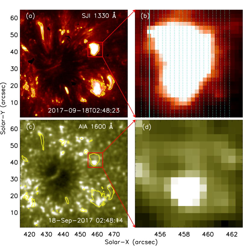
Figure 1: Left: UV images in SJI 1330 Å (a) and AIA 1600 Å (c). The yellow contours are from the SJI 1330 Å intensities. Right: Zoomed images ($\sim$8.7″$\times$8.7″) outlined by the red box in SJI 1330 Å (b) and AIA 1600 Å (d). The solid vertical line marks the slit of IRIS at the given time ($\sim$02:48:23 UT), while the dashed vertical lines mark the IRIS slits at other times.

3 Results

To investigate the evolution of this FUV bright event, a series of FUV images in SJI 1400 Å are shown in the upper panels of Figure 2. The FUV bright event displays a loop-like structure at these given panels. At the beginning ($\sim$02:48:13 UT), the bright event is not yet scanned by the slits of IRIS. Then the bright event reaches its maximum brightness at about 02:48:50 UT, and it is scanned by the IRIS slits. Finally, the FUV bright event becomes weaker and weaker, i.e., at around 02:49:27 UT and 02:50:04 UT. During this time interval, the spectral slits firstly go through the double loop legs, and then cross the loop-top region (marked by the blue horizontal line), as indicated by the vertical lines. As mentioned above, the time cadence of the IRIS/SJI is only a quarter of IRIS spectra. Therefore, each SJI image is over-plotted with four vertical lines which represent the spectral slit sites. The middle panels show the similar FUV bright event in SJI 1330 Å images. The lower panels give a series of Near Ultraviolet (NUV) images in SJI 2796 Å, which also exhibit the NUV bright event with a similar behaviors as that in SJI 1400 Å and 1330 Å.

Figure 3 shows the IRIS spectra during the FUV/NUV bright event scanned by the IRIS slits at four IRIS windows, i.e., ‘Si iv 1394 Å’, ‘Si iv 1403 Å’, ‘C ii’ and ‘Mg ii k’. Although the bright event has achieved its maximum brightness in FUV band at about 02:48:50 UT (Figure 2), the slit of IRIS scans two loop legs of the FUV/NUV bright event, which exhibits two clearly enhancements of the line cores in Si iv 1393.76 Å and 1402.77 Å (6.3$\times$10⁴ K), C ii 1334.53 Å and 1335.71 Å (2$\times$10⁴ K), i.e., the slit positions at $\sim$39″ and $\sim$43″. Then the slits of IRIS move through the main body of the FUV/NUV bright event, the line cores are continued to be enhanced. At the same time, two line wings are also enhanced simultaneously, which can be extended to more than 100 km s^-1 in both red and blue wings, as outlined by the horizontal lines in the lowest panels in Figure 3. These extended red and blue wings are similar to the bi-directional jets reported by Innes et al. (1997), which could be regarded as the reconnection event. Thus the loop-top locations marked by the horizontal lines are most likely the reconnection sites. We also note that the blue/red wings of Mg ii k (10⁴ K) line can also be nearly 100 km s^-1 (the lowest panel), indicating the reconnection event might take place from the lower chromosphere to the transition region. Therefore, it is different from the pervious transition-region explosive events (e.g., Innes et al., 1997; Huang et al., 2014), which are usually detected in the spectral lines with formation temperatures between 6$\times$10⁴ K and 7$\times$10⁵ K (Wilhelm et al., 2007).

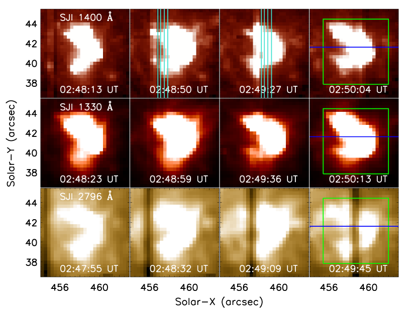
Figure 2: Snapshots in SJI 1400 Å, 1330 Å, and 2796 Å with a FOV of about 8.7″$\times$8.7″. The vertical lines mark the IRIS slits at the given snapshot. The green box outline the regions that used for the calculation of the intensities and magnetic fluxes shown in Figure 5. The horizontal lines outline the loop-top region.

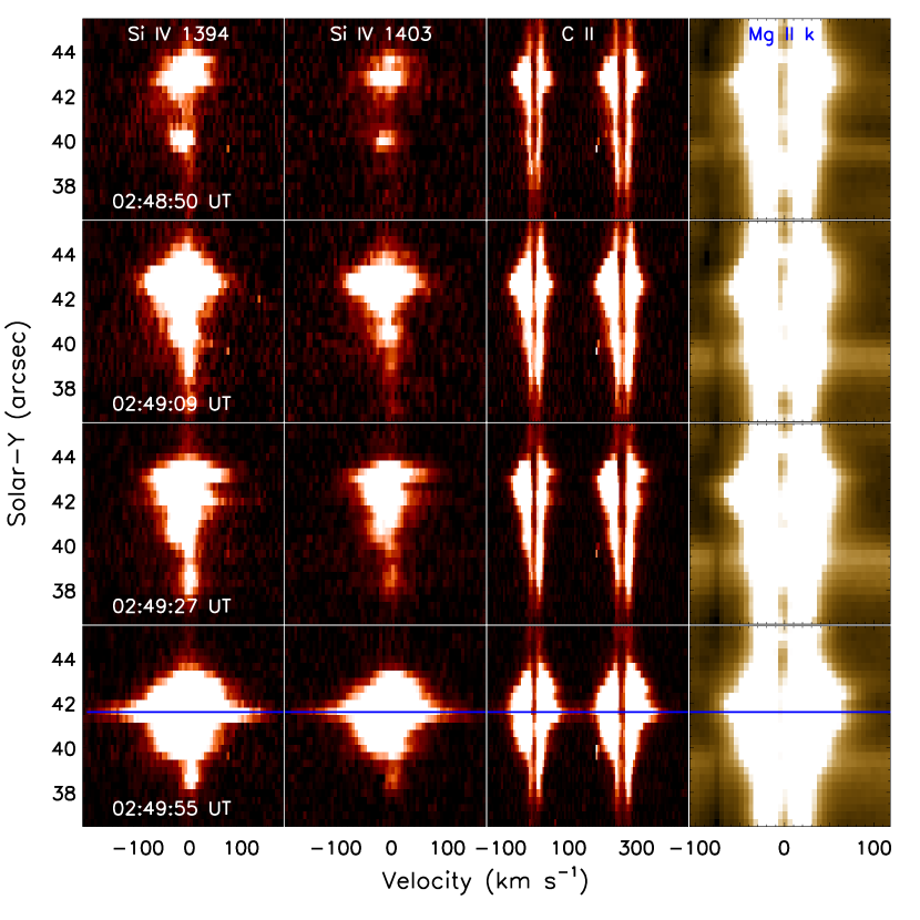
Figure 3: Simultaneous IRIS spectra of the reconnection event at the spectral windows of ‘Si iv 1394 Å’, ‘Si iv 1403 Å’, ‘C ii’ and ‘Mg ii k’, respectively. The observed times are given in the left panels. The horizontal lines outline the loop-top region in Figure 2.

To confirm this reconnection event, we then plot the line-of-sight (LOS) magnetograms from SDO/HMI (Schou et al., 2012), as shown in the upper panels of Figure 4. We can see that the loop-top region is located above the polarity inversion line between the positive and negative magnetic fields, as indicated by the red arrow and horizontal line. This observational fact suggests a possible flux cancellation of opposite magnetic polarities (Innes & Teriaca, 2013; Li et al., 2016c). On the other hand, the positive magnetic fields during the reconnection event become stronger and stronger (indicated by the red arrows), implying the flux emergence of positive magnetic field during the reconnection event (Solanki et al., 2003; Zhao et al., 2017). In contrary, the negative magnetic fields become weaker and weaker, confirming the magnetic flux cancellation. All these observational facts suggest that the evolution of magnetic fields in the photosphere provide the energy for driving the IRIS jets in the chromosphere and transition region (Peter et al., 2014; Tian et al., 2018).

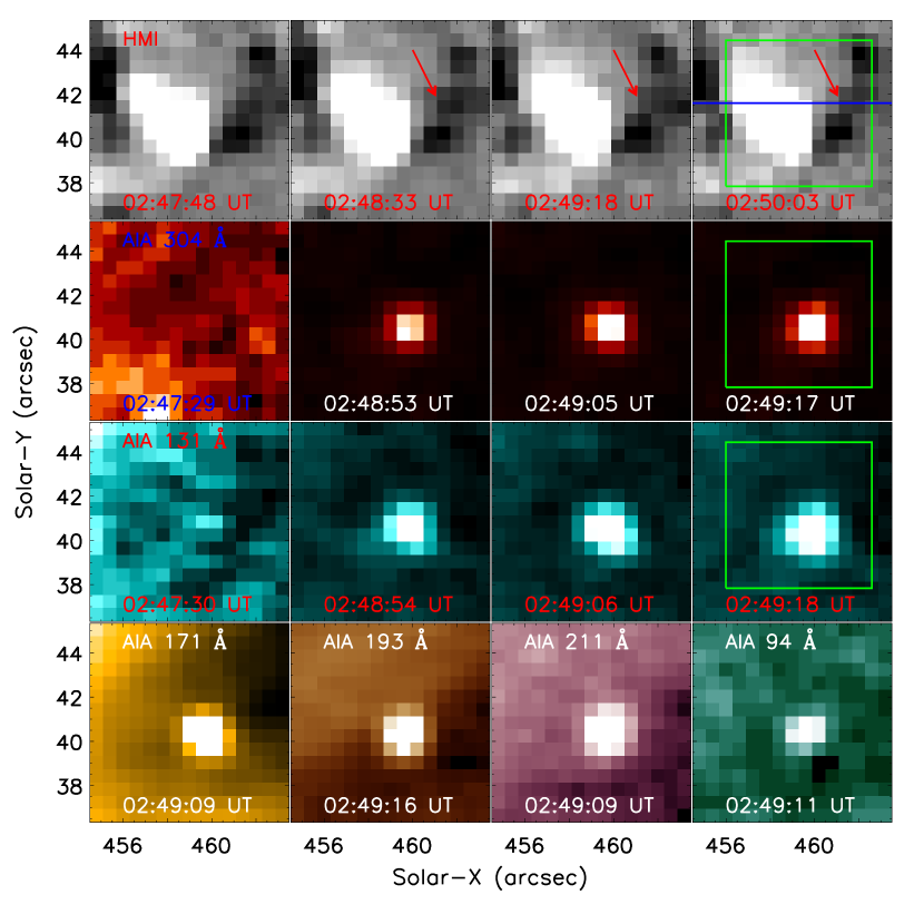
Figure 4: HMI LOS magnetograms in scale levels of $\pm$50 G, as well as AIA EUV images in 304 Å, 131 Å, 171 Å, 193 Å, and 94 Å. The green box outline the regions that used for the calculation of the intensities and magnetic fluxes shown in Figure 5. The horizontal line outlines the loop-top region in Figure 2.

To examine the response of the reconnection event in the corona, we also show the AIA images in EUV passbands in the rows 2$-$4 of Figure 4. The first-column panels in the rows of 2 and 3 display the EUV images at around 02:47 UT in AIA 304 Å and 131 Å, respectively. They does not exhibit any bright features at the reconnection event region outlined by the green box. However, both of these two channels appear to brighten in the green box region between $\sim$02:48 UT$-$02:49 UT. The other AIA EUV channels also become bright simultaneously, i.e., in AIA 171 Å, 193 Å, 211 Å, and 94 Å, as shown in the lowest panels in Figure 4. The EUV brightening from the SDO/AIA is situated closely to the reconnection sites, suggesting that the EUV brightening in the corona is caused by the magnetic reconnection which occurs in the chromosphere and transition region. All these observational facts imply that the energy that used to heat the solar corona originates from the magnetic flux cancellation in the photosphere.

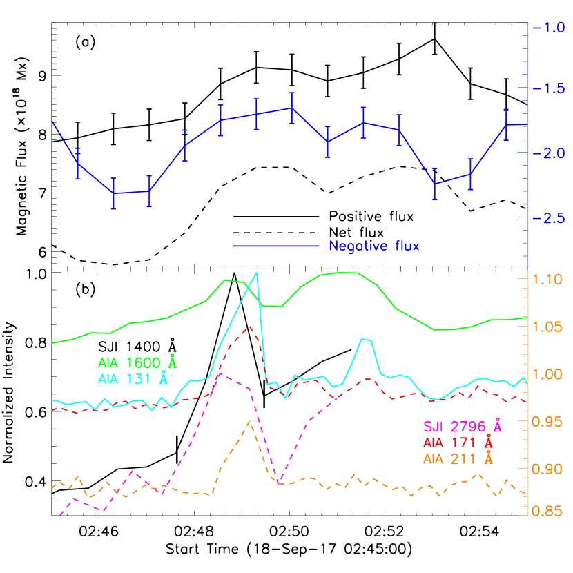
Figure 5: Panel (a): Temporal evolution of the positive (black), negative (blue) and net (dashed) magnetic fluxes from the red box given in Figure 4. The error bars ($\pm\sigma$) are given for positive and negative fluxes, respectively. Panel (b): Time series of the normalized intensity in SJI 1400 Å (black) and 12796 Å (purple), as well as AIA 1600 Å (green), 131 Å (turquoise), 171 Å (red), and 211 Å (orange). Two vertical ticks enclose the lifetime of the IRIS jets in SJI 1400 Å.

The reconnection event is identified as the flux cancellation of opposite magnetic fields in the photosphere, the IRIS jets with fast bi-directional velocities in the chromosphere and transition region, the EUV brightening in the corona. To look closely their temporal relationships, the time series of these parameters are plotted in Figure 5, the integral region is outlined with a green box in Figures 2 and 4. Panel (a) shows that the positive and net magnetic fluxes increase rapidly from $\sim$02:47 UT to $\sim$02:49 UT, and then decrease. While the negative magnetic fluxes are contrary, they greatly decrease and then grow slowly. The standard deviations ($\sigma$) of positive and negative magnetic fluxes are obtained from their time-evolution profiles, as shown by the error bars. The maximum values of the changing positive and negative fluxes are greater than their standard deviations, indicating that the changed fluxes of magnetic fields are reliable. Our observational results suggest that the rate of positive flux emergence is greater than that of flux cancellation. At the same time, the normalized intensities in SJI 1400 Å (black) and SJI 2796 Å (purple) exhibit a pronounced peak at almost the same time, as shown in panel (b). We note that double peaks appear in AIA 1600 Å flux (green), corresponding with two peaks in positive magnetic flux. However, the second peak is missed by the IRIS observations. Therefore, only the first one which corresponds to the SJI peak is studied in this paper. The same peak are also detected in EUV passbands, such as AIA 131 Å (turquoise), 171 Å (red), and 211 Å (orange). Notice that the solid lines are shown in the left axis, while the dashed lines are displayed with the right axis. It is interesting that the peak time of these EUV fluxes in SDO/AIA images is later than that of the FUV/NUV fluxes in IRIS/SJI images, indicating that the released energy in the chromosphere and transition region can spread to the overlying corona. This observational result is consistent with the traditional one-dimensional model of the solar atmosphere (Vernazza et al., 1976, 1981).

4 Discussions

To clearly illustrate that the magnetic energy in the photosphere is strong enough to drive the IRIS jets in the chromosphere and transition region and then cause the EUV brightening in the corona, the energy budgets in the solar atmospheres are given. Firstly, we estimate the released magnetic energy (E${}_{m}~{}=~{}E_{1}-E_{2}$) that derived from photospheric magnetic fields. Here, E₁ and E₂ are the total magnetic energy at the onset ($\sim$02:47 UT) and peak ($\sim$02:49 UT) times of reconnection event, respectively. They are estimated by integrating $B^{2}/8\pi$ over the area (green box) shown in the upper panels in Figure 4 with a height of $\sim$1 Mm (Sharykin et al., 2017), which is the low-limit site of this reconnection event, i.e., the height of lower chromosphere (Sturrock et al., 1986). Then considering the uncertainties of magnetic fluxes (error bars in Figure 5 a), the released magnetic energy is estimated to be about (6.7$\pm$1.9)$\times$10²⁷ erg. Next, we can estimate the kinetic energy (E${}_{k}~{}=~{}\rho Vv^{2}$) in the transition regions from the IRIS jets. Here, $\rho$ is the transition-region density ($\sim$10^-13 g cm^-3) on the Sun, $v$ is the Doppler velocity ($\sim$150 km s^-1) of Si iv 1393.76 Å line which formed in the transition region. $\frac{1}{2}$ is removed from the kinetic energy as the IRIS jets are bi-directional. The volume ($V~{}\approx~{}w^{2}~{}vt$) might be estimated by the width ($w~{}\approx$ 1″) and propagation distance ($vt$) along the LOS of the IRIS jets at its maximum speed in Figures 3 (bottom panel) and 5 (b). Here, we assume that the Doppler velocity of the IRIS jets can reach the maximum speed of $\sim$150 km s^-1 during their whole lifetime ($\sim$110 s), as shown by two vertical ticks in Figure 5 (b). Because the IRIS observational mode is scanned, we could not obtain the entire evolution of a fixed position. Therefore, the kinetic energy in the transition region estimated here is an upper-limit value, which is about 2$\times$10²⁶ erg.

We then calculate the upper limit (Aschwanden, 2005) of thermal energy (E${}_{t}~{}\approx~{}3n_{e}k_{B}T_{e}l^{3}$) in the corona from the EUV brightening. Here, a cube volume ($l^{3}$) is assumed for the EUV brightening, $n_{e}$ is the typical coronal number density ($\sim$10⁹ cm^-3, Tian et al., 2016), $k_{B}$ is Boltzmann constant, $l$ is estimated from the scale ($\sim$3″) of the EUV brightening in Figure 4. $T_{e}$ can be obtained from the differential emission measure (DEM) result using SDO/AIA data in six EUV channels (Cheng et al., 2012) at the peak brightness, which is about 1.85 MK, as shown in Figure 6. Notice that the confident temperature (log T) range is from 5.8 to 6.6, given on the uncertainties (colored rectangles) of the DEM analysis. Thus the upper limit of the thermal energy is around 7$\times$10²⁴ erg. Our results suggest that the released magnetic energy in the photosphere is big enough to drive the IRIS jets in the chromosphere and transition region, and then cause the EUV brightening in the corona, in the case that the thermal energy produced in the transition region is of the same order (10²⁶ erg) of the E_k, i.e., $E_{m}~{}\gg~{}E_{k}~{}+~{}E_{t}$.

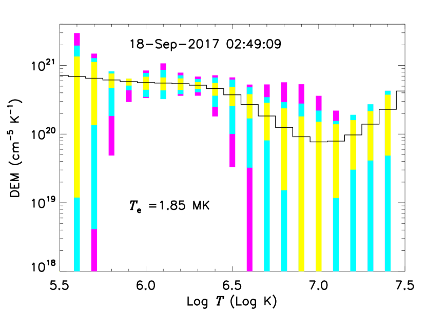
Figure 6: DEM analysis result. The black profile shows the best-fitted DEM curve from AIA observations. The yellow, turquoise, and purple rectangles represent the regions that contain 50%, 51%$-$80%, and 81%$-$95% of the Monte Carlo solutions.

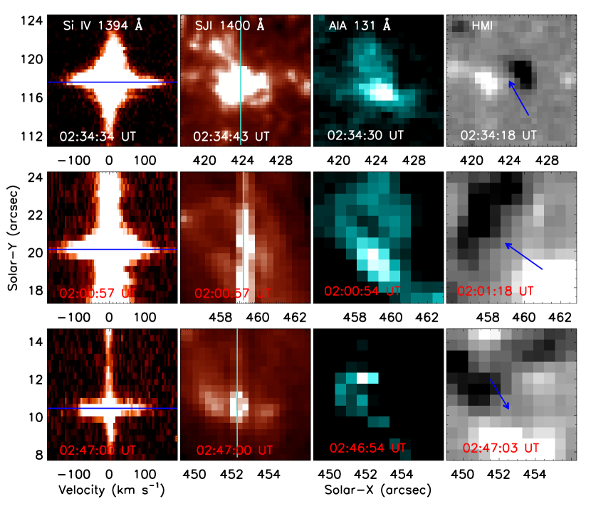
Figure 7: Three similar reconnection events during this IRIS observation.

One reconnection event is detailed studied in the previous section, it originates in the photosphere and subsequently spreads to the corona. Then more cases from the IRIS and SDO observations are found. Figure 7 shows three similar reconnection events in this IRIS FOV during its observational time. These reconnection events exhibit the same features. They are firstly identified as the IRIS jets with fast bi-directional velocities in the transition region (first column), such as the simultaneous enhancements of two extended line wings of Si iv 1393.76 Å. They all display the enhanced coronal emission, i.e., AIA 131 Å brightening (third column). Finally, all these events are located above the polarity inversion line between the positive and negative magnetic fields, as indicated by the blue arrows. Although there are a lot of transition-region and coronal enhanced events in the imaging observations, most of them are missed by the slit of IRIS. Therefore, the observations of IRIS jets with fast bi-directional velocities are rare. Likely, four such IRIS jets are observed, and the underlying photospheric magnetic field shows flux cancellation, while the overlying coronal emission appears EUV brightening, which confirm the process of magnetic reconnection from the photosphere through the chromosphere and transition region to the corona. All our observations suggest that the IRIS jets driven by the photospheric magnetic fields could light up the corona. However, due to the limitation of IRIS observations, at what percent this kind of reconnection event contributes to the coronal heating is hard to be estimated.

To illustrate the process of magnetic reconnection, a sketch is showed in Figure 8. They are firstly identified as the IRIS jets with fast bi-directional velocities in NUV and FUV lines (blue and red arrows in the middle panel), indicating that the reconnection sites are ranging from the lower chromosphere (Mg ii k) to the transition region (Si iv). On the other hand, the reconnection events originate in the photosphere, which exhibit the flux cancellation between positive and negative magnetic fields, as shown in the lower panel. They can spread to the corona and cause the EUV brightening, as shown in the upper panel. Our observations of reconnection events agree well with the 2-D reconnection model (Shibata, 1999; Priest & Forbes, 2000), the magnetic reconnection occurs at the X-point sites (i.e., chromosphere and transition region) where anti-parallel magnetic field lines converge and reconnect, and these magnetic field lines are rooted in the positive and negative fields, as shown by the purple and green curves in Figure 8. The IRIS jets could be the reconnection outflows along the LOS, which are driven by the flux cancellation in the photosphere and can cause the EUV brightening in the corona.

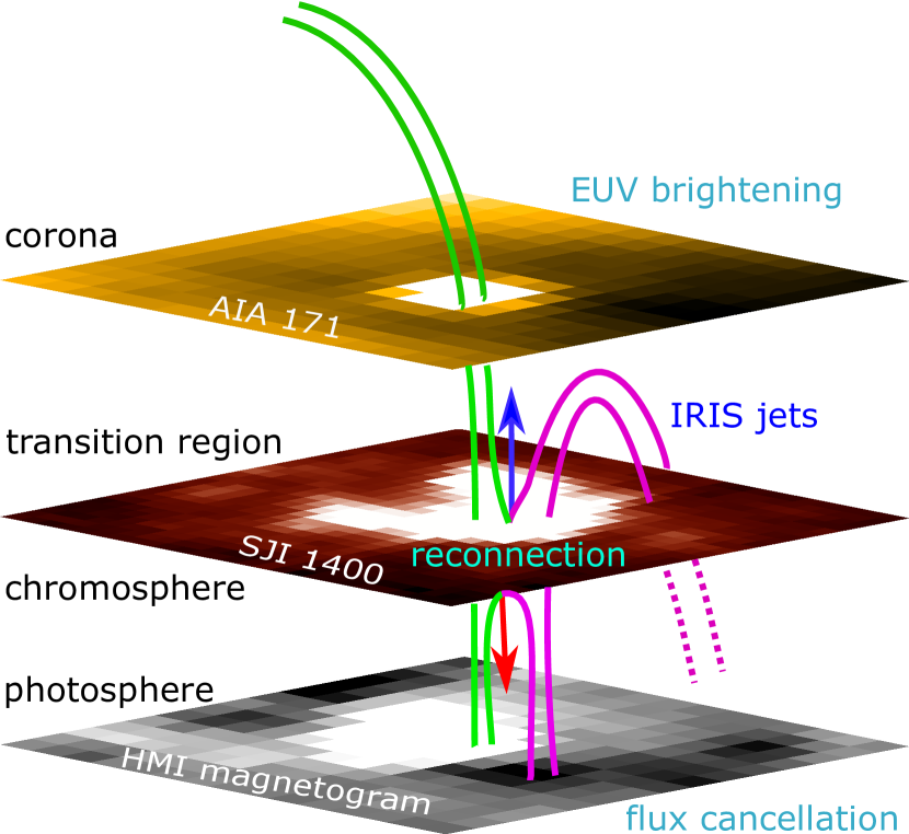
Figure 8: Sketch plot of the reconnection events. The blue and red arrows indicate the IRIS jets with bi-directions along LOS in the chromosphere and transition region. The purple and green curves represent the magnetic field lines.

There have been lots of observations of transient brightenings in the chromosphere, transition region or corona in the past four decades, i.e., the High-Resolution Telescope and Spectrograph (HRTS) rocket flights from 1979 (Dere et al., 1981), such as coronal bullets, HRTS jets, transition-region explosive events, blinkers, nanoflares, spicules, and solar tornadoes. Sometimes, they might be associated with changing magnetic field conditions in the photosphere. However, these small-scale events were only detected in one individual or two solar atmospheres at each observation, and their observations were separated to spectroscopy or image. For example, coronal bullets were observed as small and discrete ejecta of chromospheric plasmas in EUV lines, their speed could accelerate to be $\sim$450 km s^-1 (Brueckner, 1980; Karpen et al., 1984). HRTS jets changed their blueshifted and redshifted components rapidly, and the derived LOS velocities were in the range of 10$-$100 km s^-1 (Karpen et al., 1982; Brueckner & Bartoe, 1983). Transition-region explosive events were identified as non-Gaussian broadening profiles in EUV lines (Dere et al., 1991; Innes & Teriaca, 2013). Blinkers were detected as the intensity enhancements in EUV/SXR lines (Harrison, 1997; Chae et al., 2000). Nanoflares were observed as EUV brightenings in the corona (Benz & Krucker, 1998; Ishikawa et al., 2017). Spicules were dynamic jet-like features in the chromosphere or corona (Pereira et al., 2016; De Pontieu et al., 2017). Solar tornadoes were observed as tornado-like structures of magnetized plasmas in the corona (Su et al., 2012; Wedemeyer-Böhm et al., 2012). Using the spectroscopic (IRIS) and imaging (SDO/AIA and SDO/HMI) observations, the reconnection events in this study can be observed in almost all the solar atmospheres, i.e., flux cancellation in the photosphere, IRIS jets in the chromosphere and transition region, and EUV brightening in the corona, as shown in the Figure 8.

5 Summary

Using the spectroscopic and imaging observations from IRIS and SDO, we detailed report a reconnection event that firstly identify as IRIS jets in the chromosphere and transition region, which are associated with the magnetic flux cancellation in the photosphere and the EUV brightening in the corona. The IRIS jets can be detected in the spectral lines of Mg ii k, C ii and Si iv, implying that the site of magnetic reconnection is from the lower chromosphere to the transition region. The contemporaneous flux cancellation confirms the magnetic reconnection, which also indicates that the driver of the energy release lies in the photosphere. While the AIA EUV brightening suggests that the IRIS jets driven by the underlying flux cancellation can cause the overlying coronal emission. Then another three reconnection events are found during this IRIS observation, which further suggest that the origin of coronal heating lies in the photosphere and support the heating model of small-scale magnetic reconnection. Future works will focus on analyzing much more cases and performing a statistical research.

References

- Alipour & Safari (2015) Alipour, N., & Safari, H. 2015, ApJ, 807, 175
- Antolin et al. (2008) Antolin, P., Shibata, K., Kudoh, T., Shiota, D., & Brooks, D. 2008, ApJ, 688, 669
- Aschwanden (2002) Aschwanden, M. J. 2002, Space Sci. Rev., 101, 1
- Aschwanden (2005) Aschwanden, M. J. 2005, Physics of the Solar Corona (2nd ed.; Chichester: Praxis Publishing)
- Benz & Krucker (1998) Benz, A. O., & Krucker, S. 1998, Sol. Phys., 182, 349
- Brković & Peter (2004) Brković, A., & Peter, H. 2004, A&A, 422, 709
- Brueckner (1980) Brueckner, G. E. 1980, Highlights of Astronomy, 5, 557
- Brueckner & Bartoe (1983) Brueckner, G. E., & Bartoe, J.-D. F. 1983, ApJ, 272, 329
- Chae et al. (1998) Chae, J., Wang, H., Lee, C.-Y., Goode, P. R., & Schühle, U. 1998, ApJ, 504, L123
- Chae et al. (2000) Chae, J., Wang, H., Goode, P. R., Fludra, A., & Schühle, U. 2000, ApJ, 528, L119
- Cheng et al. (2012) Cheng, X., Zhang, J., Saar, S. H., & Ding, M. D. 2012, ApJ, 761, 62
- Curdt et al. (2012) Curdt, W., Tian, H., & Kamio, S. 2012, Sol. Phys., 280, 417
- De Pontieu et al. (2011) De Pontieu, B., McIntosh, S. W., Carlsson, M., et al. 2011, Science, 331, 55
- De Pontieu et al. (2014) De Pontieu, B., Title, A. M., Lemen, J. R., et al. 2014, Sol. Phys., 289, 2733
- De Pontieu et al. (2017) De Pontieu, B., De Moortel, I., Martinez-Sykora, J., & McIntosh, S. W. 2017, ApJ, 845, L18
- Dere et al. (1981) Dere, K. P., Bartoe, J.-D. F., & Brueckner, G. E. 1981, BAAS, 13, 845
- Dere et al. (1991) Dere, K. P., Bartoe, J.-D. F., Brueckner, G. E., Ewing, J., & Lund, P. 1991, J. Geophys. Res., 96, 9399
- Dere (1994) Dere, K. P. 1994, Advances in Space Research, 14, 13
- Doyle et al. (2006) Doyle, J. G., Popescu, M. D., & Taroyan, Y. 2006, A&A, 446, 327
- Grant et al. (2018) Grant, S. D. T., Jess, D. B., Zaqarashvili, T. V., et al. 2018, Nature Physics, 14, 480
- Gupta & Tripathi (2015) Gupta, G. R., & Tripathi, D. 2015, ApJ
- Harrison (1997) Harrison, R. A. 1997, Sol. Phys., 175, 467
- Heggland et al. (2009) Heggland, L., De Pontieu, B., & Hansteen, V. H. 2009, ApJ, 702, 1
- Henriques et al. (2016) Henriques, V. M. J., Kuridze, D., Mathioudakis, M., & Keenan, F. P. 2016, ApJ, 820, 124
- Hong et al. (2014) Hong, J., Jiang, Y., Yang, J., et al. 2014, ApJ, 796, 73
- Hong et al. (2017) Hong, Z.-X., Yang, X., Wang, Y., et al. 2017, Research in Astronomy and Astrophysics, 17, 25
- Huang et al. (2014) Huang, Z., Madjarska, M. S., Xia, L., et al. 2014, ApJ, 797, 88
- Innes et al. (1997) Innes, D. E., Inhester, B., Axford, W. I., & Wilhelm, K. 1997, Nature, 386, 811
- Innes & Teriaca (2013) Innes, D. E., & Teriaca, L. 2013, Sol. Phys., 282, 453
- Innes et al. (2015) Innes, D. E., Guo, L.-J., Huang, Y.-M., & Bhattacharjee, A. 2015, ApJ, 813, 86
- Ishikawa et al. (2017) Ishikawa, S.-n., Glesener, L., Krucker, S., et al. 2017, Nature Astronomy, 1, 771
- Ji et al. (2012) Ji, H., Cao, W., & Goode, P. R. 2012, ApJ, 750, L25
- Karpen et al. (1982) Karpen, J. T., Oran, E. S., Mariska, J. T., Boris, J. P., & Brueckner, G. E. 1982, ApJ, 261, 375
- Karpen et al. (1984) Karpen, J. T., Oran, E. S., & Boris, J. P. 1984, ApJ, 287, 396
- Klassen et al. (2005) Klassen, A., Krucker, S., Kunow, H., et al. 2005, Journal of Geophysical Research (Space Physics), 110, A09S04
- Klimchuk (2006) Klimchuk, J. A. 2006, Sol. Phys., 234, 41
- Lemen et al. (2012) Lemen, J. R., & Title, A. M., & Akin, D. J., et al. 2012, Sol. Phys., 275, 17
- Li et al. (2007) Li, C., Tang, Y. H., Dai, Y., Fang, C., & Vial, J.-C. 2007, A&A, 472, 283
- Li et al. (2016b) Li, D., Innes, D. E., & Ning, Z. J. 2016b, A&A, 587, A11
- Li et al. (2016c) Li, D., Ning, Z., & Su, Y. 2016c, Ap&SS, 361, 301
- Li et al. (2016a) Li, L., Zhang, J., Peter, H., et al. 2016a, Nature Physics, 12, 847
- Li et al. (2018) Li, Y., Xue, J. C., Ding, M. D., et al. 2018, ApJ, 853, L15
- Lin et al. (2005) Lin, J., Ko, Y.-K., Sui, L., et al. 2005, ApJ, 622, 1251
- Liu et al. (2010) Liu, R., Lee, J., Wang, T., et al. 2010, ApJ, 723, L28
- Longcope (1998) Longcope, D. W. 1998, ApJ, 507, 433
- Mackay et al. (2010) Mackay, D. H., Karpen, J. T., Ballester, J. L., Schmieder, B., & Aulanier, G. 2010, Space Sci. Rev., 151, 333
- Mackay & Yeates (2012) Mackay, D. H., & Yeates, A. R. 2012, Living Reviews in Solar Physics, 9, 6
- Masuda et al. (1994) Masuda, S., Kosugi, T., Hara, H., Tsuneta, S., & Ogawara, Y. 1994, Nature, 371, 495
- Mathioudakis et al. (2013) Mathioudakis, M., Jess, D. B., & Erdélyi, R. 2013, Space Sci. Rev., 175, 1
- McIntosh et al. (2011) McIntosh, S. W., de Pontieu, B., Carlsson, M., et al. 2011, Nature, 475, 477
- Ni et al. (2015) Ni, L., Kliem, B., Lin, J., & Wu, N. 2015, ApJ, 799, 79
- Ning & Guo (2014) Ning, Z., & Guo, Y. 2014, ApJ, 794, 79
- Parnell & Jupp (2000) Parnell, C. E., & Jupp, P. E. 2000, ApJ, 529, 554
- Parnell et al. (2002) Parnell, C. E., Bewsher, D., & Harrison, R. A. 2002, Sol. Phys., 206, 249
- Pesnell et al. (2012) Pesnell, W. D., Thompson, B. J., & Chamberlin, P. C. 2012, Sol. Phys., 275, 3
- Pereira et al. (2016) Pereira, T. M. D., Rouppe van der Voort, L., & Carlsson, M. 2016, ApJ, 824, 65
- Peter et al. (2014) Peter, H., Tian, H., Curdt, W., et al. 2014, Science, 346, 1255726
- Priest et al. (1994) Priest, E. R., Parnell, C. E., & Martin, S. F. 1994, ApJ, 427, 459
- Priest & Forbes (2000) Priest, E., & Forbes, T. 2000, Magnetic Reconnection, UK: Cambridge University Press
- Priest & Forbes (2002) Priest, E. R., & Forbes, T. G. 2002, A&ARv, 10, 313
- Roussev et al. (2001) Roussev, I., Galsgaard, K., Erdélyi, R., & Doyle, J. G. 2001, A&A, 370, 298
- Reale (2014) Reale, F. 2014, Living Reviews in Solar Physics, 11, 4
- Schmelz et al. (2013) Schmelz, J. T., Winebarger, A. R., Kimble, J. A., et al. 2013, ApJ, 770, 160
- Schou et al. (2012) Schou, J., Scherrer, P. H., Bush, R. I., et al. 2012, Sol. Phys., 275, 229
- Sharykin et al. (2017) Sharykin, I. N., Sadykov, V. M., Kosovichev, A. G., Vargas-Dominguez, S., & Zimovets, I. V. 2017, ApJ, 840, 84
- Shibata (1999) Shibata, K. 1999, Ap&SS, 264, 129
- Solanki et al. (2003) Solanki, S. K., Lagg, A., Woch, J., Krupp, N., & Collados, M. 2003, Nature, 425, 692
- Sturrock et al. (1986) Sturrock, P. A., Holzer, T. E., Mihalas, D. M., & Ulrich, R. K. 1986, Physics of the Sun. Volume 2, 2
- Su et al. (2012) Su, Y., Wang, T., Veronig, A., Temmer, M., & Gan, W. 2012, ApJ, 756, L41
- Su et al. (2013) Su, Y., Veronig, A. M., Holman, G. D., et al. 2013, Nature Physics, 9, 489
- Takasao et al. (2012) Takasao, S., Asai, A., Isobe, H., & Shibata, K. 2012, ApJ, 745, L6
- Tian et al. (2014) Tian, H., DeLuca, E. E., Cranmer, S. R., et al. 2014, Science, 346, 1255711
- Tian et al. (2016) Tian, H., Young, P. R., Reeves, K. K., et al. 2016, ApJ, 823, L16
- Tian et al. (2018) Tian, H., Zhu, X., Peter, H., et al. 2018, ApJ, 854, 174
- Tsuneta et al. (1992) Tsuneta, S., Hara, H., Shimizu, T., et al. 1992, PASJ, 44, L63
- Vernazza et al. (1976) Vernazza, J. E., Avrett, E. H., & Loeser, R. 1976, ApJS, 30, 1
- Vernazza et al. (1981) Vernazza, J. E., Avrett, E. H., & Loeser, R. 1981, ApJS, 45, 635
- Wedemeyer-Böhm et al. (2012) Wedemeyer-Böhm, S., Scullion, E., Steiner, O., et al. 2012, Nature, 486, 505
- Wilhelm et al. (2007) Wilhelm, K., Marsch, E., Dwivedi, B. N., & Feldman, U. 2007, Space Sci. Rev., 133, 103
- Winebarger et al. (2002) Winebarger, A. R., Emslie, A. G., Mariska, J. T., & Warren, H. P. 2002, ApJ, 565, 1298
- Xue et al. (2016) Xue, Z., Yan, X., Cheng, X., et al. 2016, Nature Communications, 7, 11837
- Yan et al. (2018a) Yan, X. L., Yang, L. H., Xue, Z. K., et al. 2018a, ApJ, 853, L18
- Yan et al. (2018b) Yan, L., Peter, H., He, J., Xia, L., & Wang, L. 2018b, A&A, 611, A49
- Yang et al. (2015) Yang, S., Zhang, J., & Xiang, Y. 2015, ApJ, 798, L11
- Yokoyama et al. (2001) Yokoyama, T., Akita, K., Morimoto, T., Inoue, K., & Newmark, J. 2001, ApJ, 546, L69
- Young et al. (2013) Young, P. R., Doschek, G. A., Warren, H. P., & Hara, H. 2013, ApJ, 766, 127
- Young et al. (2018) Young, P. R., Tian, H., Peter, H., et al. 2018, arXiv:1805.05850
- Zhang et al. (2001) Zhang, J., Kundu, M. R., & White, S. M. 2001, Sol. Phys., 198, 347
- Zhang et al. (2012) Zhang, Q. M., Chen, P. F., Guo, Y., Fang, C., & Ding, M. D. 2012, ApJ, 746, 19
- Zhao et al. (2017) Zhao, J., Schmieder, B., Li, H., et al. 2017, ApJ, 836, 52