An integral transform technique for kinetic systems with collisions

Abstract

The linearized Vlasov-Poisson system can be exactly solved using the $G$-transform, an integral transform introduced in Refs. Morrison and Pfirsch, 1992; Morrison, 1994, 2000 that removes the electric field term, leaving a simple advection equation. We investigate how this integral transform interacts with the Fokker-Planck collision operator. The commutator of this collision operator with the $G$-transform (the “shielding term”) is shown to be negligible. We exactly solve the advection-diffusion equation without the shielding term. This solution determines when collisions dominate and when advection (i.e.  Landau damping) dominates. This integral transform can also be used to simplify gyro-/drift-kinetic equations. We present new gyrofluid equations formed by taking moments of the $G$-transformed equation. Since many gyro-/drift-kinetic codes use Hermite polynomials as basis elements, we include an explicit calculation of their $G$-transform.

I Introduction

One of the intriguing features of the Vlasov-Poisson system is the ability of an electrostatic wave to damp, even in the absence of any dissipation mechanism.Landau (1946) This can occur because the electrostatic wave couples to a continuum of modes describing all of the possible ways that the distribution function can vary in velocity space.

The linearized Vlasov-Poisson system can be solved using the Laplace transform,Landau (1946); Lenard and Bernstein (1958) normal modes,van Kampen (1955) a Green’s function,Thompson (1962); Callen (2014) or numerically by a variety of codes (e.g. Refs. Cheng and Knorr, 1976; Heath et al., 2012; Pezzi et al., 2016; Kraus et al., 2017). Another method for describing Landau damping, which employs an integral transform in velocity space based on the Hilbert transform, was introduced in Refs. Morrison and Pfirsch, 1992; Morrison, 1994, 2000. Applying this $G$-transform to the linearized Vlasov-Poisson equation completely removes the electric field term. The resulting advection equation is trivially solved, and then the inverse transform is applied to return the solution to the original coordinates.

Versions of this integral transform exist for a variety of models,Morrison (2003) and there is one that can be used effectively on any collisionless kinetic model with one velocity dimension.

A simple and important way to extend the linearized Vlasov-Poisson system is to add collisions. The Landau-Boltzmann collision operator for Coulomb collisions is usually unmanageable, so simpler collision operators are often used instead. A good collision operator, such as the Fokker-Planck operator,Rayleigh (1891); Fokker (1914); Chandrasekhar (1943); Lenard and Bernstein (1958); Degond and Lucquin-Desreux (1992) acts as a diffusion in velocity space, conserves particle number, and has a Maxwellian equilibrium. Typically, the collision frequency is assumed to be small. Even if the collision frequency is small, collisions shouldn’t be completely neglected. Landau damping produces fine structures in velocity space for which the diffusion eventually becomes important.

The picture of Landau damping is similar to Kolmogorov turbulence: energy which is input on large velocity scales cascades down to smaller velocity scales until it reaches a dissipation velocity scale where the collisions are important. There is also an intermediate velocity scale where collisions are important for particles with small parallel velocities.White and Hazeltine (2017) Since the damping rate typically depends more on the creation of fine structures in velocity space than on the details of the collision operator, replacing the complete collision operator with a simplified version is reasonable. Landau damping causes the effective dissipation rate to be much higher than the collision frequency. The importance of the fine structures in determining the dissipation rate can be seen by noticing that if the initial conditions have fine structures in velocity space, then the damping rate can be much higher than if the initial conditions differ from a Maxwellian in a more gradual way.Pezzi et al. (2016)

Gyrokinetics and drift-kinetics are a natural places to look for applications for the $G$-transform because they have only one velocity dimension. In many applications, the plasma has a strong magnetic field. A particle’s motion perpendicular to this field mostly follows small circles around the field lines. This motion does not need to be resolved. Instead, the three-dimensional Vlasov-Poisson equations are integrated over the perpendicular velocity dimensions. Drift velocities which depend on the fields can be added to preserve the important aspects of the perpendicular motion. The resulting system has three spatial dimensions, one velocity dimension and time. Frieman and Chen (1982); Brizard and Hahm (2007); Krommes (2012)

The $G$-transform has been used to analyze data from laboratory experiments.Sarfaty et al. (1996); Skiff et al. (2000, 2002); Skiff (2002) Doppler-resolved laser induced fluorescence measures the dependence of the distribution function on the velocity parallel to the laser beam. $G$-transforming the data at a single point yields the amplitudes of the van Kampen modes excited by an externally created wave. The spatial dependence of the electric field can be determined from the van Kampen mode amplitudes using a measurement of the velocity distribution function at a single point. The $G$-transform could also be used on satellite data to measure Landau damping and nonlinear energy transfer between fields and particles in the heliosphere.Howes et al. (2016, 2018)

The paper is organized as follows. In Sec. II we review general properties of the $G$-transform and its use on the one-dimensional linearized Vlasov-Poisson system. This is followed by Sec. III that deals with collisions. Here we show that the $G$-transform almost commutes with the collision operator. The resulting equations have an exact solution which allows us to easily compare advection and diffusion. These results are robust to changes in initial conditions or the collision operator. Sec. IV shows how the $G$-transform can also be used to simplify gyro-/dirft-kinetic equations. The resulting equations, which no longer have a parallel electric field, can be solved numerically using a basis of Hermite polynomials or we can take moments of them to get novel drift-fluid equations. We conclude in Sec. V.

II One-Dimensional Vlasov-Poisson

One of the simplest models for a plasma is the one-dimensional Vlasov equation for a single species plasma,

$$\frac{\partial f}{\partial t}+v\frac{\partial f}{\partial x}-\frac{e}{m}\frac{\partial\phi}{\partial x}\frac{\partial f}{\partial v}=0\,,$$ (1)

where the electric field is determined self-consistently using the Poisson equation,

$$\nabla^{2}\phi=4\pi e\int_{\mathbb{R}}fdv-4\pi\rho_{b}\,,$$ (2)

with $e$ and $m$ being the electron charge and mass, respectively, and $\rho_{b}$ being a neutralizing background positive charge density. Linearizing (1) and (2) about an arbitrary homogeneous equilibrium, $n_{0}f_{0}(v)$ and Fourier transforming the perturbation in position, yields

$$\frac{\partial f_{k}}{\partial t}+ikv\,f_{k}-i\,\frac{\omega_{P}^{2}}{k}\int_{\mathbb{R}}f_{k}\,dv^{\prime}\,\frac{df_{0}}{dv}=0,$$ (3)

which we consider for an arbitrary initial conditions $\overset{\circ}{f_{k}}(v)$. In (3) the third term comes from substituting the linearized Poisson equation in for the electric field, and the second term will be refereed to as the advection term.

Equation (3) can be exactly solved using the $G$-transform, which relies on the Hilbert transform. So we review it and some of its properties next.

II.1 Hilbert Transform Properties

The Hilbert Transform is defined by

$$H[g](v):=\frac{1}{\pi}\mathchoice{{\vbox{\hbox{$\textstyle-$ }}\kern-6.52776pt}}{{\vbox{\hbox{$\scriptstyle-$ }}\kern-4.91667pt}}{{\vbox{\hbox{$\scriptscriptstyle-$ }}\kern-3.95833pt}}{{\vbox{\hbox{$\scriptscriptstyle-$ }}\kern-3.54166pt}}\!\!\int_{\mathbb{R}}\frac{g(u)}{u-v}\,du,$$ (4)

where $\mathchoice{{\vbox{\hbox{$\textstyle-$ }}\kern-6.52776pt}}{{\vbox{\hbox{$\scriptstyle-$ }}\kern-4.91667pt}}{{\vbox{\hbox{$\scriptscriptstyle-$ }}\kern-3.95833pt}}{{\vbox{\hbox{$\scriptscriptstyle-$ }}\kern-3.54166pt}}\!\!\int$ is the Cauchy principle part of the integral. Following is a list of some basic Hilbert transform properties, with well-known proofs (see e.g. Ref. King, 2009):

$$\bullet\ \ H[\ldots]\ \mathrm{is\ a\ linear\ operator.}$$ (5)

$$\bullet\ \ \mathrm{If}\ g(v)\ \mathrm{has\ a\ Hilbert\ transform,\ then\ there\ is\ a\ function}$$

$$\qquad G,\ \mathrm{analytic\ in\ the\ upper\ half\ complex}\ v-\mathrm{plane,\ that}$$

$$\qquad\mathrm{limits\ to\ the\ real}\ v\ \mathrm{axis\ with}$$

$$\qquad g(v)=g_{R}(v)+ig_{I}(v),$$ (6)

$$\qquad\mathrm{where\ the\ real\ and\ imaginary\ parts\ of}\ G\ \mathrm{are\ related\ by}$$

$$\qquad g_{R}=H[g_{I}]\ ,\hskip 30.00005ptg_{I}=-H[g_{R}]\,.$$ (7)

$$\bullet\ \ \mathrm{The\ inverse\ of\ the\ Hilbert\ transform\ is\ negative\ itself,\ i.e.}$$

$$\qquad H[H[g]]=-g\,.$$ (8)

$$\bullet\ \ \mathrm{For\ two\ functions}\ g_{1}\ \mathrm{and}\ g_{2},\ \mathrm{the\ following\ convolution}$$

$$\qquad\mathrm{identity\ holds:}$$

$$\qquad H[g_{1}H[g_{2}]+g_{2}H[g_{1}]]=H[g_{1}]H[g_{2}]-g_{1}g_{2}\,.$$ (9)

$$\bullet\ \ \mathrm{The\ Hilbert\ transform\ commutes\ with\ differentiation,\ i.e.}$$

$$\qquad H\left[\frac{\partial g}{\partial u}\right]=\frac{\partial}{\partial v}H[g]\,.$$ (10)

$$\bullet\ \ \mathrm{The\ Hilbert\ transform\ has\ the\ following\ multiplication}$$

$$\qquad\mathrm{by}\ u\ \mathrm{identity:}$$

$$\qquad H[ug]=vH[g]+\frac{1}{\pi}\mathchoice{{\vbox{\hbox{$\textstyle-$ }}\kern-6.52776pt}}{{\vbox{\hbox{$\scriptstyle-$ }}\kern-4.91667pt}}{{\vbox{\hbox{$\scriptscriptstyle-$ }}\kern-3.95833pt}}{{\vbox{\hbox{$\scriptscriptstyle-$ }}\kern-3.54166pt}}\!\!\int_{\mathbb{R}}g(u)\ du\,.$$ (11)

$$\bullet\ \ \mathrm{The\ adjoint\ of\ the\ Hilbert\ transform\ is\ negative\ itself,\ i.e.}$$

$$\qquad\mathchoice{{\vbox{\hbox{$\textstyle-$ }}\kern-6.52776pt}}{{\vbox{\hbox{$\scriptstyle-$ }}\kern-4.91667pt}}{{\vbox{\hbox{$\scriptscriptstyle-$ }}\kern-3.95833pt}}{{\vbox{\hbox{$\scriptscriptstyle-$ }}\kern-3.54166pt}}\!\!\int_{\mathbb{R}}f\ H[g]\ dv=-\mathchoice{{\vbox{\hbox{$\textstyle-$ }}\kern-6.52776pt}}{{\vbox{\hbox{$\scriptstyle-$ }}\kern-4.91667pt}}{{\vbox{\hbox{$\scriptscriptstyle-$ }}\kern-3.95833pt}}{{\vbox{\hbox{$\scriptscriptstyle-$ }}\kern-3.54166pt}}\!\!\int_{\mathbb{R}}g\ H[f]\ dv\,.$$ (12)

$$\bullet\ \ \mathrm{The\ Hilbert\ transform\ reverses\ the\ parity\ of\ a\ function,\ i.e.}$$

$$\qquad\mathbf{\Pi}\Big{[}H[f]\Big{]}=-\mathbf{\Pi}[f]\,.$$ (13)

Of interest in plasma physics is that fact that the Hilbert transform of a Gaussian is the real part of the plasma Z function, i.e.

$$Z\left(\frac{u}{v_{t}}\right) := \pi H\left[\frac{1}{\sqrt{\pi}}e^{-v^{2}/v_{t}^{2}}\right]$$ (14)

$$= \frac{1}{\sqrt{\pi}}\mathchoice{{\vbox{\hbox{$\textstyle-$ }}\kern-6.52776pt}}{{\vbox{\hbox{$\scriptstyle-$ }}\kern-4.91667pt}}{{\vbox{\hbox{$\scriptscriptstyle-$ }}\kern-3.95833pt}}{{\vbox{\hbox{$\scriptscriptstyle-$ }}\kern-3.54166pt}}\!\!\int_{\mathbb{R}}e^{-v^{2}/v_{t}^{2}}\frac{dv}{v-u}\,.$$

From Hilbert transform properties (10) and (11) and from our knowledge of the derivative of a Gaussian, we can determine that the derivative of the plasma Z function satisfies:

$$\frac{\partial Z}{\partial u} = -\frac{2}{v_{t}}\left(1+\frac{u}{v_{t}}Z\left(\frac{u}{v_{t}}\right)\right)\,.$$ (15)

II.2 $G$-Transform and Exact Linear Solution

The $G$-transform is defined by

$$f(v)=G[g](v):=\epsilon_{R}(v)g(v)+\epsilon_{I}(v)H[g](v)\,,$$ (16)

where

$$\epsilon_{I}(v):=-\pi\frac{\omega_{P}^{2}}{k^{2}}\frac{\partial f_{0}(v)}{\partial v}\ \mbox{and}\ \epsilon_{R}(v):=1+H[\epsilon_{I}](v).$$ (17)

In order for an integral transform to be useful, it has to have an inverse, which for this one is given by

$$g(u)=G^{-1}[f](u):=\frac{\epsilon_{R}(u)}{|\epsilon(u)|^{2}}f(u)-\frac{\epsilon_{I}(u)}{|\epsilon(u)|^{2}}H[f](u)\,,$$ (18)

where $|\epsilon|^{2}:=\epsilon_{R}^{2}+\epsilon_{I}^{2}$. It is straightforward to check that $g(u)=G^{-1}[G[g]](u)$ using the definition of $\epsilon_{R}$ (17) and Hilbert transform properties (8) and (9).

The $G$-transform provides an exact solution to the one-dimensional linear Vlasov equation. Morrison and Pfirsch (1992); Morrison (1994, 2000) The transform takes you to new coordinates that naturally unravel the phase mixing. In these new coordinates, there is no term from the electric field, so the equation is trivial.

Apply the inverse $G$-transform in velocity space to (3) gives

$$\frac{\partial}{\partial t}G^{-1}[f_{k}]+ik\,G^{-1}[vf_{k}]$$

$$\hskip 56.9055pt-i\frac{\omega_{P}^{2}}{k}\int_{\mathbb{R}}f_{k}dv^{\prime}\,G^{-1}\left[\frac{df_{0}}{dv}\right]=0\,.$$ (19)

Defining $g_{k}:=G^{-1}[f_{k}]$, the first term is simple, while the other two terms will take a little bit of work.

The second term can be dealt with using Hilbert transform property (11). The correction term is the integral of a nonsingular quantity, so we can remove the principal value from the integral,

$$G^{-1}[vf_{k}(v)] = \frac{\epsilon_{R}}{|\epsilon|^{2}}uf_{k}(u)-\frac{\epsilon_{I}}{|\epsilon|^{2}}H[vf_{k}(v)]$$ (20)

$$= \frac{\epsilon_{R}}{|\epsilon|^{2}}uf_{k}(u)$$

$$\quad-\frac{\epsilon_{I}}{|\epsilon|^{2}}\left(uH[f_{k}(v)]+\frac{1}{\pi}\mathchoice{{\vbox{\hbox{$\textstyle-$ }}\kern-6.52776pt}}{{\vbox{\hbox{$\scriptstyle-$ }}\kern-4.91667pt}}{{\vbox{\hbox{$\scriptscriptstyle-$ }}\kern-3.95833pt}}{{\vbox{\hbox{$\scriptscriptstyle-$ }}\kern-3.54166pt}}\!\!\int_{\mathbb{R}}f_{k}(v)dv\right)$$

$$= u\left(\frac{\epsilon_{R}}{|\epsilon|^{2}}f_{k}(u)-\frac{\epsilon_{I}}{|\epsilon|^{2}}H[f_{k}(v)]\right)$$

$$\quad-\frac{1}{\pi}\frac{\epsilon_{I}}{|\epsilon|^{2}}\int_{\mathbb{R}}f_{k}(v)dv$$

$$= u\,G^{-1}[f_{k}]-\frac{\epsilon_{I}}{\pi|\epsilon|^{2}}\int_{\mathbb{R}}f_{k}(v)dv\,.$$

The third term can be dealt with by recognizing that ${df_{0}}/{dv}$ is only a constant away from $\epsilon_{I}$ and that $H[\epsilon_{I}]=\epsilon_{R}-1$. Thus,

$$G^{-1}\left[\frac{df_{0}}{dv}\right] = G^{-1}\left[-\frac{k^{2}}{\pi\omega_{P}^{2}}\,\epsilon_{I}\right]=-\frac{k^{2}}{\pi\omega_{P}^{2}}G^{-1}[\epsilon_{I}]$$ (21)

$$= -\frac{k^{2}}{\pi\omega_{P}^{2}}\left(\frac{\epsilon_{R}}{|\epsilon|^{2}}\epsilon_{I}-\frac{\epsilon_{I}}{|\epsilon|^{2}}(\epsilon_{R}-1)\right)$$

$$= -\frac{k^{2}}{\pi\omega_{P}^{2}}\frac{\epsilon_{I}}{|\epsilon|^{2}}\,.$$

Upon plugging these results back into (19) we observe the remarkable cancellation

$$\frac{\partial g_{k}}{\partial t} = -ik\left(ug_{k}-\frac{\epsilon_{I}}{\pi|\epsilon|^{2}}\int_{\mathbb{R}}f_{k}dv\right)$$ (22)

$$\qquad+\ i\frac{\omega_{P}^{2}}{k}\int_{\mathbb{R}}f_{k}dv^{\prime}\left(-\frac{k^{2}}{\pi\omega_{P}^{2}}\frac{\epsilon_{I}}{|\epsilon|^{2}}\right)$$

$$= -ikug_{k}\,.$$

The solution of (22) is trivial,

$$g_{k}(u,t)=\overset{\circ}{g_{k}}(u)\,e^{-ikut}\,.$$ (23)

The one-dimensional linear Vlasov equation can be solved by first inverse $G$-transforming the initial conditions to get $\overset{\circ}{g_{k}}(u)$, using the solution (23), and then $G$-transforming back into the original coordinates,

$$f_{k}(v,t)=G\left[G^{-1}[\overset{\circ}{f_{k}}(v)]\,e^{-ikut}\right]\,.$$ (24)

It can be shown that this solution is equivalent to van Kampen’s solution, which in turn is equivalent to Landau’s.

II.3 Landau Damping

Evidently, the solution of (24) must include Landau damping. If the equilibrium distribution function is monotonically decreasing, then the spatial dependence of a perturbation (associated with the electric field) decays. How does Landau damping appear in this solution?

The distribution function itself doesn’t damp - it could not because this is a Hamiltonian system. Instead, what damps are the density and electrical field perturbations, which are proportional to the integral of the distribution function. For example,

$$n_{k}(t) = \int_{\mathbb{R}}G\left[G^{-1}[\overset{\circ}{f_{k}}](u)\,e^{-ikut}\right]dv$$

$$= \int_{\mathbb{R}}\left(\epsilon_{R}(v)\,G^{-1}[\overset{\circ}{f_{k}}](v)\ e^{-ikvt}\right.$$

$$+ \left.\epsilon_{I}(v)\,\frac{1}{\pi}\,\mathchoice{{\vbox{\hbox{$\textstyle-$ }}\kern-6.52776pt}}{{\vbox{\hbox{$\scriptstyle-$ }}\kern-4.91667pt}}{{\vbox{\hbox{$\scriptscriptstyle-$ }}\kern-3.95833pt}}{{\vbox{\hbox{$\scriptscriptstyle-$ }}\kern-3.54166pt}}\!\!\int_{\mathbb{R}}G^{-1}[\overset{\circ}{f_{k}}](u)\,e^{-ikut}\frac{du}{u-v}\right)dv$$

$$= \int_{\mathbb{R}}dv\,\epsilon_{R}(v)\,G^{-1}[\overset{\circ}{f_{k}}](v)\ e^{-ikvt}$$

$$+ \frac{1}{\pi}\,\mathchoice{{\vbox{\hbox{$\textstyle-$ }}\kern-6.52776pt}}{{\vbox{\hbox{$\scriptstyle-$ }}\kern-4.91667pt}}{{\vbox{\hbox{$\scriptscriptstyle-$ }}\kern-3.95833pt}}{{\vbox{\hbox{$\scriptscriptstyle-$ }}\kern-3.54166pt}}\!\!\int_{\mathbb{R}}du\int_{\mathbb{R}}dv\ \frac{1}{u-v}\epsilon_{I}(v)\,G^{-1}[\overset{\circ}{f_{k}}](u)\ e^{-ikut}\,.$$

Because the integrals in (II.3), including the integrals in the $G^{-1}$-transform, are not simple, we will only look for the damping in the long time limit.

The Riemann-Lebesgue lemma determines the long time limit; for any sufficiently smooth function $F(\zeta)$,

$$\lim\limits_{t\rightarrow\infty}\int_{\mathbb{R}}F(\zeta)\,e^{-i\zeta t}\,d\zeta=0\,.$$ (26)

The integrals in (II.3) are of the form specified in the Riemann-Lebesgue Lemma, if we assume that the initial conditions are sufficiently smooth and $|\epsilon|^{2}$ is never zero along the real axis. We can thus conclude,

$$\lim\limits_{t\rightarrow\infty}n_{k}(t)=0\,.$$ (27)

The density perturbation of the plasma (and thus the electric field) decays to zero as time $\rightarrow\infty$. The Riemann-Lebesgue Lemma also tells us that the decay rate will be proportional to the distance from the real axis to the nearest pole of $F(\zeta)$. In our case, that is the distance from the real axis to the nearest place where $|\epsilon|^{2}=0$. From this one can obtain the usual damping rate.Morrison and Pfirsch (1992)

III Collisions

Let us now consider collisions together with the Vlasov-Poisson dynamics by adding a collision operator to the right-hand side of (3),

$$\frac{\partial f_{k}}{\partial t}+ikvf_{k}-i\frac{\omega_{P}^{2}}{k}\int_{\mathbb{R}}f_{k}dv^{\prime}\frac{df_{0}}{dv}=\mathcal{C}[f]\,.$$ (28)

Equation (28) is no longer Hamiltonian. A manifestation of this is that any good the collision operator $\mathcal{C}[f]$, will have asymptotic stability to a Maxwellian distribution. A common choice for describing collisions is the Fokker-Planck operator,Rayleigh (1891); Fokker (1914); Chandrasekhar (1943); Lenard and Bernstein (1958); Degond and Lucquin-Desreux (1992) that has the form

$$\mathcal{C}[f]:=\nu\left(\frac{v_{t}^{2}}{2}\frac{\partial^{2}f_{k}}{\partial v^{2}}+v\frac{\partial f_{k}}{\partial v}+f_{k}\right)\,.$$ (29)

This operator gives zero when it acts on the Maxwellian

$$f_{0}(v)=\frac{1}{\sqrt{\pi}v_{t}}e^{-v^{2}/v_{t}^{2}}.$$ (30)

If the advection and electric field terms are set to zero, then any other initial function of velocity will decay to this Maxwellian.

Without collisions we had a continuum of possible equilibria, but adding the Fokker-Planck collision operator selects (30) as the only equilibrium. Thus we no longer work with general $\epsilon_{I}(v)$ and $\epsilon_{R}(v)$ - instead we can be content with a special case of the Maxwellian, where

$$\epsilon_{I} = \sqrt{\pi}\,\frac{2\omega_{P}^{2}}{k^{2}v_{t}^{2}}\,\frac{v}{v_{t}}\,e^{-v^{2}/v_{t}^{2}}$$ (31)

$$\epsilon_{R} = 1+\frac{2\omega_{P}^{2}}{k^{2}v_{t}^{2}}+\frac{2\omega_{P}^{2}}{k^{2}v_{t}^{2}}\,\frac{v}{v_{t}}\,Z\left(\frac{v}{v_{t}}\right)\,.$$ (32)

In (32) $Z$ is the real part of the plasma Z function of (14).

If $\nu$ is small, we might be tempted to treat the collision operator as a perturbation on the original problem. This is not easy because we are faced with a singular perturbation. The small parameter multiplies the highest derivative of $f$ with respect to $v$. If $f$ has structure on extremely small velocity scales, then the highest derivative of $f$ can become $O(1/\nu)$, making a conventional perturbation theory illegitimate. For the Vlasov-Poisson system, we are guaranteed that $f$ will eventually get fine structure in $v$, since it behaves as $e^{-ikut}$ for large $t$.

This motivates our use of the $G$-transform to attack this problem.

III.1 $G$-Transform and Collisions

Now, let us apply the inverse $G$-transform in velocity space to (28). Because we have already seen the cancellation that occurs with the Vlasov part of this equation, we need only examine its affect on the collision operator, which leads to

$$\frac{\partial g_{k}}{\partial t}+ikug_{k}=G^{-1}\left[\mathcal{C}[G[g_{k}]]\right]\,.$$ (33)

We will have to determine the commutation relations between the $G$-transform and the collision operator. Before doing so we state some properties of the collision operator. The proofs are all simple and some indications of how to approach them are given immediately after each.

$$\bullet\ \ \mathcal{C}[\ldots]\ \mathrm{is\ a\ linear\ operator.}$$ (34)

$$\bullet\ \ \mathcal{C}[\epsilon_{I}]=-\nu\epsilon_{I}.$$ (35)

$$\qquad\mathrm{Recall}\ \epsilon_{I}\propto{df_{0}}/{dv}\propto v\ \exp({-v^{2}/v_{t}^{2}})\ \mathrm{and\ consider}$$

$$\qquad\mathrm{the\ derivatives\ of\ this.}$$

$$\bullet\ \ \mathcal{C}[AB]=B\,\mathcal{C}[A]+A\,\mathcal{C}[B]-\nu AB+\nu v_{t}^{2}\frac{\partial A}{\partial v}\frac{\partial B}{\partial v}.$$ (36)

$$\qquad\mathrm{Use\ the\ product\ rule\ several\ times\ and\ rearrange.}$$

$$\bullet\ \ \mathcal{C}[H[A]]=H[\mathcal{C}[A]].$$ (37)

$$\qquad\mathrm{Use\ Hilbert\ transform\ properties\ \eqref{HDeriv}\ and\ \eqref{Hu},\ and}$$

$$\qquad\mathrm{note\ everything\ decays\ at}\ \infty.$$

$$\bullet\ \ \mathcal{C}[\epsilon_{R}]=\nu(2-\epsilon_{R}).$$ (38)

$$\qquad\mathrm{Use\ the\ definition\ of}\ \epsilon_{R}\ \mathrm{of\ \eqref{EpsDefinition}\ and\ collision}$$

$$\qquad\mathrm{operator\ property\ \eqref{CollEpsI}.}$$

In order to evaluate $\mathcal{C}[G[g_{k}]]$, we first use the linearity property (34),

$$\mathcal{C}[G[g_{k}]]=\mathcal{C}[\epsilon_{R}g_{k}]+\mathcal{C}[\epsilon_{R}H[g_{k}]]\,.$$ (39)

Next we use the collision operator product rule (36) on each term, and then apply the collision operator on $\epsilon_{I}$ using property (35) and on $\epsilon_{R}$ using property (38),

$$\mathcal{C}[\epsilon_{R}g_{k}] = \epsilon_{R}\mathcal{C}[g_{k}]+g_{k}\mathcal{C}[\epsilon_{R}]-\nu\epsilon_{R}g_{k}+\nu v_{t}^{2}\frac{\partial\epsilon_{R}}{\partial v}\frac{\partial g_{k}}{\partial v}$$

$$= \epsilon_{R}\mathcal{C}[g_{k}]+2\nu(1-\epsilon_{R})g_{k}+\nu v_{t}^{2}\frac{\partial\epsilon_{R}}{\partial v}\frac{\partial g_{k}}{\partial v}\,,$$

$$\mathcal{C}[\epsilon_{I}H[g_{k}]] = \epsilon_{I}\mathcal{C}[H[g_{k}]]+H[g_{k}]\mathcal{C}[\epsilon_{I}]-\nu\epsilon_{I}H[g_{k}]$$ (40)

$$\hskip 56.9055pt+\nu v_{t}^{2}\frac{\partial\epsilon_{I}}{\partial v}\frac{\partial H[g_{k}]}{\partial v}$$

$$= \epsilon_{I}H[\mathcal{C}[g_{k}]]-2\nu\epsilon_{I}H[g_{k}]$$

$$\hskip 56.9055pt+\nu v_{t}^{2}\frac{\partial\epsilon_{I}}{\partial v}H\left[\frac{\partial g_{k}}{\partial u}\right]\,.$$

We can also commute the collision operator with the Hilbert transform using property (37), and note that a derivative can move inside of a Hilbert transform using Hilbert transform property (10). Thus we obtain

$$\mathcal{C}[G[g_{k}]] = \epsilon_{R}\mathcal{C}[g_{k}]+2\nu(1-\epsilon_{R})g_{k}+\nu v_{t}^{2}\frac{\partial\epsilon_{R}}{\partial v}\frac{\partial g_{k}}{\partial v}$$

$$+\epsilon_{I}H[\mathcal{C}[g_{k}]]-2\nu\epsilon_{I}H[g_{k}]+\nu v_{t}^{2}\frac{\partial\epsilon_{I}}{\partial v}H\left[\frac{\partial g_{k}}{\partial u}\right]$$

$$= \big{(}\epsilon_{R}\mathcal{C}[g_{k}]+\epsilon_{I}H[\mathcal{C}[g_{k}]]\big{)}+2\nu g_{k}$$

$$\hskip 45.52458pt-2\nu(\epsilon_{R}g_{k}+\epsilon_{I}H[g_{k}])$$

$$\hskip 45.52458pt+\nu v_{t}^{2}\left(\frac{\partial\epsilon_{R}}{\partial v}\frac{\partial g_{k}}{\partial v}+\frac{\partial\epsilon_{I}}{\partial v}H\left[\frac{\partial g_{k}}{\partial u}\right]\right)$$

$$= G[\mathcal{C}[g_{k}]]+2\nu(g_{k}-G[g_{k}])$$

$$\hskip 45.52458pt+\nu v_{t}^{2}\left(\frac{\partial\epsilon_{R}}{\partial v}\frac{\partial g_{k}}{\partial v}+\frac{\partial\epsilon_{I}}{\partial v}H\left[\frac{\partial g_{k}}{\partial u}\right]\right)\,.$$

Using this result in (33), we can determine how the collision operator interacts with the $G$-transform,

$$\frac{\partial g_{k}}{\partial t}+ikug_{k} = G^{-1}\left[\mathcal{C}[G[g_{k}]]\right]$$

$$= G^{-1}\bigg{[}G[\mathcal{C}[g_{k}]]+2\nu(g_{k}-G[g_{k}])$$

$$+\nu v_{t}^{2}\left(\frac{\partial\epsilon_{R}}{\partial v}\frac{\partial g_{k}}{\partial v}+\frac{\partial\epsilon_{I}}{\partial v}H\left[\frac{\partial g_{k}}{\partial u}\right]\right)\bigg{]}$$

$$= \mathcal{C}[g_{k}]+2\nu G^{-1}[g_{k}]-\nu g_{k}$$

$$+2\nu v_{t}^{2}\,G^{-1}\bigg{[}\left(\frac{\partial\epsilon_{R}}{\partial v}\frac{\partial g_{k}}{\partial v}+\frac{\partial\epsilon_{I}}{\partial v}H\left[\frac{\partial g_{k}}{\partial u}\right]\right)\bigg{]}\,.$$

When dealing with the $G^{-1}$ of the last term, we use Hilbert transform property (9) to simplify the $H[...H[...]]$ term.

Finally, we obtained the $G$-transformed one-dimensional Vlasov equation with collisions:

$$\frac{\partial g_{k}}{\partial t}+ikug_{k} = \mathcal{C}[g_{k}]+2\nu(G^{-1}[g_{k}]-g_{k})$$ (44)

$$+ \frac{\nu v_{t}^{2}}{|\epsilon|^{2}}\bigg{[}\left(\epsilon_{R}\frac{\partial\epsilon_{R}}{\partial u}-\epsilon_{I}\frac{\partial\epsilon_{I}}{\partial u}\right)\frac{\partial g_{k}}{\partial u}$$

$$+ \left(\epsilon_{R}\frac{\partial\epsilon_{I}}{\partial u}+\epsilon_{I}\frac{\partial\epsilon_{R}}{\partial u}\right)H\left[\frac{\partial g_{k}}{\partial v}\right]\bigg{]}\,.$$

The left hand side of this equation is simply advection: the electric field term has vanished. The right-hand side of this equation has the collision operator in terms of $u$, but it also has other terms. The rest of the right-hand side describes how the electric field and the collisions interact. We will call all of them the shielding term, $\mathcal{S}[g_{k}]$.

III.2 Dropping the Shielding Term

What have we gained by doing the $G^{-1}$-transformation?

At first, it doesn’t look like we’ve gained very much. If the collision operator isn’t there, the $G$-transform transforms an integro-differential equation into a differential equation. The equations of motion are dramatically simpler since they are local in $k$ and $v$. However, the shielding term that arises from the $G$-transform of the collision operator is also nonlocal. We have replaced an integro-differential equation with another integro-differential equation. And, the new one looks more complicated.

However, if we know that some terms are small, it is a reasonable approximation to drop all of the complicated terms on the right-hand side and add them in later as a perturbation.

In most physical situations when the Vlasov equation is relevant, the collision frequency $\nu$ is assumed to be smaller than the other frequencies in the system.

$$\nu g_{k}\ll\frac{\partial g_{k}}{\partial t}\ ,\ kug_{k}$$ (45)

All of the terms on the right-hand side are proportional to $\nu$, so they all appear to be smaller than the terms on the left hand side of (44). This suggests that it might be possible to treat the collision term as a perturbation in the original problem and not worry about $G$-transforming the collision operator.

Having a small collision frequency is not enough to make sure that the right-hand side remains small. The collision operator has a term proportional to ${\partial^{2}g_{k}}/{\partial u^{2}}$, which is the highest derivative with respect to $u$ in the problem. Although the left hand side may be originally dominant, the dynamics create small-scale structure in velocity space, with terms proportional to $\exp({ikvt})$. These small scales in velocity space make the collision operator significant, even for small collision frequencies.

Note, unlike the Fourier transform, the Hilbert transform preserves scale. If g(u) = H[f(v)](u) and $f$ is rapidly varying, say $f(v/\lambda)$ for $\lambda<<1$, then $g(u/\lambda)$. Thus rapid variation is also preserved by the $G$-transform: a solution with a rapid scale of variation $\exp({ikut})$ in $u$ will have a scale of variation $\exp({ikvt})$ in $v$, and vice versa.

The highest derivative in the shielding term is ${\partial g_{k}}/{\partial u}$. When a function has extremely small scales, its higher order derivatives are larger than its lower order derivatives. Even when the right-hand side of this equation is important, the collision operator still dominates the shielding term.

This same argument could also be used for the last two terms of the collision operator (29). They both are also multiplied by the small parameter $\nu$ and neither has a second derivative. If we are justified in dropping the shielding terms, then we are also justified in dropping the latter two terms of the collision operator.

We thus have two reasonable approximations that we could make: drop the shielding terms and keep the entire collision operator or drop everything except the second derivative. We call the second derivative by itself $\mathcal{D}[g_{k}]$ for diffusion and everything else can be lumped together into an expanded set of shielding terms $\mathcal{S}^{\prime}[g_{k}]$.

If we keep only the second derivative, the resulting solution is easier to solve and analyze analytically. However, it’s long-time limit is strange. The full collision operator relaxes to a Maxwellian with width $v_{t}$. The collision operator $\mathcal{D}$ results in a Gaussian whose width increases without bound. This is not too big of a concern for us since our perturbations will decay on a much shorter time than the collision time $1/\nu$. Numerically, these ever-expanding tails cause problems at the boundary. When we consider the problem numerically in Sec. III.7, we use the entire collision operator. A comparison of the analytic solutions for both of these reasonable approximations in found in Appendix A. The two solutions agree anywhere they are significantly different from zero.

The shielding term is a good term to initially ignore, and then add back in as a perturbation.

III.3 Exact Solution of the Advection-Diffusion Equation

Given the arguments of Sec. III.2, we proceed with the local equation:

$$\frac{\partial g_{k}}{\partial t}+ikug_{k}=\nu\frac{v_{t}^{2}}{2}\frac{\partial^{2}g_{k}}{\partial u^{2}}\,,$$ (46)

an equation that can be exactly solved. First Fourier transform in velocity. This reduces the equation to being first order in time and velocity instead of being first order in time and second order in velocity. We can then use the method of characteristics to solve this problem with the Fourier transformed initial conditions. Afterwards, we inverse Fourier transform back into the original velocity coordinate. Instead of working through this calculation, we will just state the solution. For more details, see Sec. III.8, where we consider the corresponding inhomogeneous problem. Given the equation (46) and an initial condition which is Gaussian in velocity and has a wave number $k$ in position,

$$g_{k}(u,0)=\frac{1}{\sqrt{\pi}v_{t}}e^{-{u^{2}}/{v_{t}^{2}}}\,,$$ (47)

the solution to (46) is

$$g(u,t) = \frac{1}{\sqrt{\pi}v_{t}\sqrt{1+2\nu t}}\exp\bigg{[}-\frac{u^{2}}{v_{t}^{2}\,(1+2\nu t)}$$

$$-ikut\,\frac{1+\nu t}{1+2\nu t}-\frac{1}{12}k^{2}v_{t}^{2}\nu t^{3}\,\frac{2+\nu t}{1+2\nu t}\bigg{]}\,.$$

As a check, it is not difficult to plug this solution back into the equations and see that it does satisfy them. An existence and uniqueness theorem guarantees that this is the only correct solution.

The exponential of (III.3) has three terms. The first term is the result of the diffusion part of the equation. If we ignore advection here, the remaining heat equation will cause a Gaussian to spread out in time. The variance in velocity space increases, but the amplitude of the perturbation does not change. The time scale for this process is $1/\nu$. In our ordering, the perturbation will already have decayed away before this increased variance becomes significant.

The second term is primarily the result of the advection part of the equation. It is a velocity dependent phase shift of the initial conditions. This doesn’t change the amplitude of the perturbation to the distribution function. As we saw in Sec. II.3, it does result in Landau damping for the perturbation to the density and electric field.

The rate at which this occurs is modulated by an extra factor resulting from the collision operator. This factor is unity at $t=0$ and decays to $1/2$ as $t\rightarrow\infty$. This change occurs with a time scale $1/\nu$, so the perturbation will already have damped away before its effect becomes significant. However, as we will see in Sec. III.5, this effect can occur much sooner for other initial conditions.

The third term is the result of the interaction between the two terms. It is also where the damping of the perturbation to the distribution function comes from. Neither term individually damps the distribution function, but their interaction does.

This term is modulated by a factor which varies from $2$ at $t=0$ to $1/2$ as $t\rightarrow\infty$. The time scale over which this happens is $1/\nu$, so it will be close to $2$ until the perturbation has almost entirely decayed.

If we define the decay time, $t_{D}$, for this equation to be the time for the perturbation to the distribution function to decay to $1/e$ of its original value, and then approximate the modulating factor to be $2$, we find

$$-1=-\frac{1}{6}k^{2}v_{t}^{2}\nu t_{D}^{3}\ \Rightarrow\ t_{D}=\left(\frac{6}{k^{2}v_{t}^{2}\nu}\right)^{1/3}\,.$$ (49)

Since this goes as $\nu^{-1/3}$, this time is much shorter than the time scale associated with the collisions by themselves. Callen also found an effective damping rate which scales as the (parallel) collision frequency to the $1/3$ when considering a similar problem.Callen (2014)

III.4 Advection-Diffusion Crossover

We can take our solution and plug it back into each of the terms of (44). Doing so will tell us when each of the terms dominates - when advection dominates the damping and when collisions dominate the damping.

It is easy to evaluate the terms in (46) on the solution:

$$\mathcal{A}[g_{k}] = iku\,g_{k}$$ (50)

$$\mathcal{D}[g_{k}] = \frac{\nu}{(1+2\nu t)^{2}}\Big{(}2\frac{u^{2}}{v_{t}^{2}}-\frac{1}{2}v_{t}^{2}k^{2}t^{2}(1+\nu t)^{2}$$ (51)

$$\quad-(1+2\nu t)+2ikut(1+\nu t)\Big{)}\,g_{k}\,,$$

whence we can calculate the ratio of the diffusion term to the advection term. Nondimensionalizing the result using $\varepsilon=\nu/kv_{t}$ , $\tau=kv_{t}t$ , and $\xi=u/v_{t}$ gives

$$\frac{\mathcal{D}[g_{k}]}{\mathcal{A}[g_{k}]} = \frac{-i\,\varepsilon}{\xi(1+2\varepsilon\tau)^{2}}\Big{(}2\xi^{2}-\frac{1}{2}\tau^{2}(1+\varepsilon\tau)^{2}$$ (52)

$$-(1+2\varepsilon\tau)+2i\xi\tau(1+\varepsilon\tau)\Big{)}\,.$$

In Fig. 1, we plot the magnitude of the ratio of (52) for various nondimensionalized times and velocities to see when each term dominates and when the two terms are comparable. For this plot, we fix $\varepsilon=0.1$.

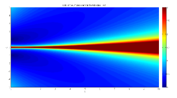
Figure 1: The magnitude of the ratio of the collision term to the advection term, plotted as a function of non-dimensional time and velocity, respectively.

The advection term dominates for small times and large velocities. The collision term dominates for large times and small velocities. For sufficiently large velocities, the collisions start becoming important again, but the distribution function is so small at these velocities that this isn’t significant.

III.5 Other Initial Conditions

The perturbation to the distribution function could be a very different temperature than the equilibrium temperature that appears in the collision operator. Let us choose as an initial condition in $u$ a Gaussian with a different initial thermal velocity, say $v_{I}$,

$$g_{k}(u,0)=\frac{1}{\sqrt{\pi}v_{I}}e^{-{u^{2}}/{v_{I}^{2}}}\,.$$ (53)

The calculation proceeds as before. Upon defining $\alpha:=v_{I}^{2}/v_{t}^{2}$, we find

$$g(u,t) = \frac{1}{\sqrt{\pi}v_{t}\sqrt{\alpha+2\nu t}}\exp\bigg{[}-\frac{u^{2}}{v_{t}^{2}\,(\alpha+2\nu t)}$$

$$-ikut\,\frac{\alpha+\nu t}{\alpha+2\nu t}-\frac{1}{12}v_{t}^{2}k^{2}\nu t^{3}\,\frac{2\alpha+\nu t}{\alpha+2\nu t}\bigg{]}\,.$$

This has the same asymptotic behavior as before, but the time it takes for the modulation factors to transition from close to unity to close to $1/2$ is now $\alpha/\nu$. This transition is observable if this time is shorter than the decay time, i.e.

$$\frac{\alpha}{\nu}\lesssim t_{D}\ \Rightarrow\ \frac{v_{I}}{v_{t}}\lesssim\left(\frac{\nu}{kv_{t}}\right)^{1/3}\,.$$ (55)

In order to measure the modulation of the phase mixing term, you have to use initial conditions with thermal velocities much smaller than the equilibrium thermal velocity.

We could also consider initial conditions in $u$ that are a polynomial times a Gaussian. The calculation proceeds as before - the only difference is that there is now a polynomial multiplying everything. The solution will also be (III.3), multiplied by some polynomial in $u$ and $t$.

An appropriately chosen set of polynomials, such as the Hermite polynomials, will form a complete basis. Any other bounded function that decays quickly enough in velocity can be written as a superposition of these functions. Our analysis of the solution in Sec. III.3 also applies for many initial conditions.

III.6 Realistic Initial Conditions

Gaussian initial conditions in velocity are not physically realistic in $u$ space. The initial conditions (47) are commonly used in kinetics because they represent a purely spatial perturbation to the distribution function. We have transformed the velocity coordinate, so we should use different initial conditions for the advection-diffusion equation, viz.

$$\overset{\circ}{g_{k}}(u)=G^{-1}\left[\overset{\circ}{f_{k}}(v)\right]=G^{-1}\left[\frac{1}{\sqrt{\pi}v_{t}}e^{-{v^{2}}/{v_{t}^{2}}}\right].$$ (56)

We assume that the thermal velocity for the equilibrium is the same as the thermal velocity of the initial conditions. We’ve already calculated $\epsilon_{I}$ (31) and $\epsilon_{R}$ (32). Thus the initial condition of (56) in $G^{-1}$-transformed space is

$$\overset{\circ}{g_{k}}(u) = \frac{\frac{1}{\sqrt{\pi}v_{t}}e^{-u^{2}/v_{t}^{2}}(1+\frac{2\omega_{P}^{2}}{k^{2}v_{t}^{2}})}{A^{2}+B^{2}}\,,$$ (57)

where

$$A := \sqrt{\pi}\frac{2\omega_{P}^{2}}{k^{2}v_{t}^{2}}\frac{u}{v_{t}}e^{-u^{2}/v_{t}^{2}}$$

$$B := 1+\frac{2\omega_{P}^{2}}{k^{2}v_{t}^{2}}+\frac{2\omega_{P}^{2}}{k^{2}v_{t}^{2}}\frac{u}{v_{t}}Z({u}/{v_{t}})\,.$$ (58)

We will use (57) in Sec. III.7.

III.7 Numerically Comparing Advection and Diffusion

Instead of trying to deal with the initial conditions (57) analytically, we solved the advection-diffusion equation with the entire collision operator (105) numerically using a finite difference method. Our code is written in MATLAB, and is simple enough to be run on a personal laptop.

A Gaussian equilibrium distribution function,

$${f_{0}}(v)=\frac{1}{\sqrt{\pi}v_{t}}e^{-v^{2}/v_{t}^{2}}\,,$$

with units in velocity and position where $v_{t}=1$ and $k=2\pi$ was chosen. In the code we used 200 cells in $x$ with periodic boundary conditions and 200 cells in $v$ that range between $\pm 2.5v_{t}$ with Dirichlet boundary conditions. In our units of time, the collision frequency is $\nu=0.1$ and the plasma frequency is $\omega_{P}=5$. Our time step was $0.01$ and we ran the advection-diffusion equation until $t=2$, at which point the initial perturbation had almost completely decayed. The decay time (49) for these parameters is $t_{D}=1.15$. The non-dimensional parameters for this run are

$$\frac{kv_{t}}{\nu}=20\pi\ ,\ \frac{\omega_{P}}{\nu}=50.$$ (59)

To construct the realistic initial conditions (57), we used MATLAB’s built in Hilbert transform to numerically apply the $G^{-1}$-transform to Gaussian initial conditions in the original coordinates. Any other initial conditions for the original coordinates could be similarly numerically $G^{-1}$ transformed. After finding the solution, we numerically apply the $G$-transform to get the solution in the original velocity coordinate.

We emphasize that our finite difference solution of the advection-diffusion equation did not include the shielding term since it should be small. This assumption is checked below.

We can compare the sizes of various terms in both the original coordinates and in the $G^{-1}$-transformed coordinates. In both velocity coordinates, there is a time derivative, an advection term, and a Fokker-Planck collision operator. Even though the terms look the same, the solution is different in the two coordinates, so we will get different results when we evaluate the term on the solution. The original coordinates also have a term from the electric field and the transformed coordinates also have the shielding term.

We take the solution for the advection-diffusion equation and evaluate it on all of the terms in both coordinates. The shielding term, evaluated on the solution calculated without it, should be small. We also $G$-transform the shielding term evaluated on the solution back into the original coordinates, so we can see how significant what we neglected is there.

We $L^{1}$ integrate all of these terms in both position and velocity and plot the resulting magnitudes of each as a function of time in Fig. 2.

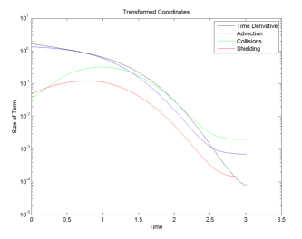
(a)  

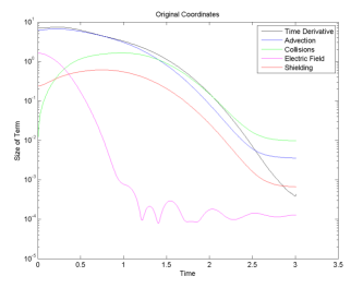
(b)  

Figure 2: The time dependence of each of the terms of the collisional Vlasov equation, $L^{1}$ integrated in position and velocity. (a) In the $G^{-1}$-transformed coordinates, there are four terms: a time derivative, an advection term, a Fokker-Planck collision operator, and the shielding term. Neglecting the shielding term when finding the solution is justified since the shielding term is always at least an order of magnitude smaller than the dominant term. (b) In the original coordinates, there are four terms: a time derivative, an advection term, a Fokker-Planck collision operator, and an electric field term. We also $G$-transformed the shielding term evaluated on the solution to see how significant the dropped term is. It is always at least an order of magnitude below the dominant term.

For small times, the advection term is dominant in both the original and transformed coordinates. In the original coordinates, the electric field term is the same order of magnitude as the advection term. One way that we could have reached the (local) advection-diffusion equation is by dropping the electric field terms and not $G$-transforming. We see here that this plan is illegitimate. Increasing the plasma frequency increases the significance of the electric field at small times.

For large times, the collision term is dominant in both the original and transformed coordinates. This is unsurprising since the advection term creates small scale structures in velocity space. The collision operator has the highest order velocity derivative in the equation, so it becomes more significant when there is lots of small scale structure.

At an intermediary time, there is a crossover where collisions replace advection as the dominant term.

The shielding term is always at least an order of magnitude lower than the other terms. This gives us confidence that neglecting it is reasonable.

III.8 Introducing the Shielding Term as a Perturbation

Since we know that the shielding terms and part of the collision operator will be small compared to the other terms, we can stick a small parameter, $\delta$, in front of these terms and write the solution $g$ as a series in this parameter,

$$g_{k}=g_{k}^{(0)}+\delta g_{k}^{(1)}+\delta^{2}g_{k}^{(2)}+\cdots\,.$$ (60)

The resulting hierarchy of equations reads

$$\frac{\partial g_{k}^{(0)}}{\partial t}+ikug_{k}^{(0)} = \mathcal{D}[g_{k}^{(0)}]$$ (61)

$$\frac{\partial g_{k}^{(1)}}{\partial t}+ikug_{k}^{(1)} = \mathcal{D}[g_{k}^{(1)}]+\mathcal{S}^{\prime}[g_{k}^{(0)}]$$ (62)

$$\frac{\partial g_{k}^{(2)}}{\partial t}+ikug_{k}^{(2)} = \mathcal{D}[g_{k}^{(2)}]+\mathcal{S}^{\prime}[g_{k}^{(1)}]$$

$$\vdots$$

where $\mathcal{D}$ and $\mathcal{S}^{\prime}$ were defined in Sec. III.2.

The zeroth order equation is the one solved above. All of the equations of other orders are inhomogeneous versions of the one solved above. The only addition is a known function of velocity, determined by the lower order solutions, added to the right-hand side.

The initial conditions of the higher order terms are all taken to be zero, i.e., the initial conditions are entirely included in the zeroth order equation.

Upon Fourier transforming in velocity space, $u\rightarrow\eta$, letting $\hat{g}:=\mathcal{F}[g_{k}^{(n)}]$ and $\hat{S}:=\mathcal{F}[\mathcal{S}^{\prime}[g_{k}^{(n-1)}]]$ gives

$$\frac{\partial\hat{g}}{\partial t}+k\frac{\partial\hat{g}}{\partial\eta}+\frac{1}{2}\nu v_{t}^{2}\eta^{2}\hat{g}=\hat{S}(\eta)\,.$$ (64)

We solve (64) using the method of characteristics, leading to the following set of differential equations for $t(r,s),\eta(r,s),$ and $\hat{g}(r,s)$:

$$\frac{dt}{ds} = 1\,,\qquad\frac{d\eta}{ds}=k,$$ (65)

$$\frac{d\hat{g}}{ds} = -\frac{1}{2}\nu v_{t}^{2}\eta^{2}\hat{g}+\hat{S}(\eta)$$ (66)

$$t(r,0) = 0\,,\qquad\eta(r,0)=r\,,\quad\hat{g}(r,0)=0$$ (67)

These equations are straightforward to solve. The first two are trivial,

$$t(r,s)=s,\hskip 20.00003pt\eta(r,s)=ks+r\,.$$ (68)

Next we plug these into the equation for $\hat{g}(r,s)$, and solve it using an integrating factor. Since we explicitly know what $\eta(r,s)$ is, we can evaluate the integrals in the exponentials. We cannot evaluate the integral $ds^{\prime\prime}$ unless we specify explicitly what $\mathcal{F}[\mathcal{S}^{\prime}[g_{k}^{(0)}]]$ is. Thus,

$$\frac{d}{ds}\left[\hat{g}\,e^{-\nu\frac{v_{t}^{2}}{2}\int\limits_{0}^{s}\eta^{2}(s^{\prime})ds^{\prime}}\right] = e^{-\nu\frac{v_{t}^{2}}{2}\int\limits_{0}^{s}\eta^{2}(s^{\prime}))ds^{\prime}}\,\hat{S}(\eta(s))$$

$$\hat{g}(r,s) = e^{\nu\frac{v_{t}^{2}}{2}\int\limits_{0}^{s}\eta^{2}(s^{\prime})ds^{\prime}}\int\limits_{0}^{s}e^{-\nu\frac{v_{t}^{2}}{2}\int\limits_{0}^{s^{\prime\prime}}\eta^{2}(s^{\prime\prime\prime})ds^{\prime\prime\prime}}\hat{S}(\eta(s^{\prime\prime}))\,ds^{\prime\prime}$$ (69)

$$= \exp\Big{[}\frac{\nu v_{t}^{2}}{6k}(k^{3}s^{3}+3k^{2}s^{2}r+3ksr^{2})\Big{]}$$

$$\times\int\limits_{0}^{s}\exp\Big{[}-\frac{\nu v_{t}^{2}}{6k}(k^{3}s^{\prime\prime 3}+3k^{2}s^{\prime\prime 2}r+3ks^{\prime\prime}r^{2})\Big{]}$$

$$\qquad\times\,\hat{S}(ks^{\prime\prime}+r)\,ds^{\prime\prime}\,.$$

We now invert (68) to get $s(t,\eta)$ and $r(t,\eta)$,

$$s=t,\hskip 20.00003ptr=\eta-kt\,,$$ (70)

and substitute these in to get $\hat{g}(\eta,t)$. Note that we do not substitute anything in for $s^{\prime\prime}$ since it is the integration variable. From this point onward, we refer to it as $s$. With the above we obtain

$$\hat{g}(\eta,t) = \exp\Big{[}\frac{\nu v_{t}^{2}}{6k}(3\eta^{2}kt-3\eta k^{2}t^{2}+k^{3}t^{3})\Big{]}$$ (71)

$$\times\int\limits_{0}^{t}\exp\Big{[}-\frac{\nu v_{t}^{2}}{6k}(3\eta^{2}ks-3\eta k^{2}s^{2}+k^{3}s^{3})\Big{]}$$

$$\qquad\times\,\hat{S}(\eta+k(s-t))\,ds\,.$$

Finally the inverse Fourier transform of (71) in velocity space yields $g_{k}^{(1)}(v,t)$. We will not write this out explicitly since our expressions are long enough already.

The higher order corrections can be done using exactly the same technique.

III.9 Other Collision Operators

The strategy for any collision operator is the same. We show that the commutator between the collision operator and the $G$-transform is small, then neglect it. The dramatic simplification of the left hand side only creates a small correction of the right-hand side.

If we choose some local collision operator with a finite number of velocity derivatives, say

$$Q_{n}[g_{k}]:=c\frac{\partial^{n}}{\partial v^{n}}g_{k}+\mathcal{O}\left[\frac{\partial}{\partial v}\right]^{n-1}g_{k}\,,$$ (72)

then we may consider how this collision operator acts on the $G$-transform.

$$Q_{n}[G[g_{k}]] = c\frac{\partial^{n}}{\partial v^{n}}\Big{(}\epsilon_{R}g_{k}+\epsilon_{I}H[g_{k}]\Big{)}+\mathcal{O}\left[\frac{\partial}{\partial v}\right]^{n-1}g_{k}$$ (73)

$$= \epsilon_{R}c\frac{\partial^{n}g_{k}}{\partial v^{n}}+\epsilon_{I}H\left[c\frac{\partial^{n}g_{k}}{\partial v^{n}}\right]+\mathcal{O}\left[\frac{\partial}{\partial v}\right]^{n-1}g_{k}$$

$$= G\left[c\frac{\partial^{n}g_{k}}{\partial v^{n}}\right]+\mathcal{O}\left[\frac{\partial}{\partial v}\right]^{n-1}g_{k}$$

$$= G[Q_{n}[g_{k}]]+\mathcal{O}\left[\frac{\partial}{\partial v}\right]^{n-1}g_{k}$$

The commutator between $Q_{n}$ and $G$ is $\mathcal{O}\left[{\partial}/{\partial v}\right]^{n-1}g_{k}$. As long as the original collision operator is multiplied by a small collision frequency, this shielding term will always be much smaller than either the advection term or the collision term. It can be neglected. The only problems could arise when $g_{k}$ is close to the kernal of $Q_{n}$ and the velocity is small.

IV Gyrokinetics and Drift-Kinetics

A three-dimensional highly magnetized plasma is often approximated by gyrokinetic or drift-kinetic equations. Frieman and Chen (1982); Brizard and Hahm (2007); Krommes (2012) We consider small electrostatic perturbations around an equilibrium with slab geometry - the equilibrium has no electric field and the magnetic field is constant and pointed in the $z$ direction. The motion of the ions is driven by an equilibrium density and temperature gradient in the $x$ direction, while the motion of the electrons is determined by quasineutrality. Since most of the particles’ motion is gyration about magnetic field, we can integrate over the gyrophase and use the adiabatic invariance of the magnetic moment to reduce the number of velocity dimensions to one: the velocity along the magnetic field lines. To make this approximation, we have to assume that the equilibrium fields do not vary on a length scale shorter than the Larmor radius and that the relevant time scales are long compared to the Larmor frequency. The perturbed quantities are allowed to vary on a length scale comparable to the Larmor radius, so the $\vec{E}\times\vec{B}$ nonlinearity is significant.

The system obtained by the above approximations is the subject of ongoing numerical studies. Hatch et al. (2014); Schekochihin et al. (2016) Specifically, the equations, in three spatial dimensions, one velocity dimension, and time, are

$$\frac{\partial f}{\partial t}+v\frac{\partial f}{\partial z}+\frac{\partial\varphi}{\partial z}\,vF_{M}+\frac{1}{2}\rho_{i}v_{t}\ [\varphi,f]_{x,y}=\mathcal{C}[f]+\chi\,,$$ (74)

where $\rho_{i}={mv_{t}}/({eB})$,

$$\varphi=\frac{ZT_{e}}{T_{i}}\int f\,dv\,,\quad F_{M}=\frac{1}{\sqrt{\pi}v_{t}}e^{-v^{2}/v_{t}^{2}}\,,$$ (75)

and

$$\chi=\left(-\frac{\rho_{i}v_{t}}{2}\frac{\partial\varphi}{\partial y}\right)\!\left(\frac{1}{L_{n}}+\left(\frac{v^{2}}{v_{t}^{2}}-\frac{1}{2}\right)\frac{1}{L_{T}}\right)F_{M},$$ (76)

with $L_{n},L_{T}$ being length scales for density and temperature gradients, respectively. The nonlinear Poisson bracket term of (74) is the perpendicular advective derivative, i.e.,

$$\vec{V}_{\perp}\cdot\nabla_{\perp}f = \frac{1}{2}\rho_{i}v_{t}\left(\hat{z}\times\nabla_{\perp}\varphi\right)\cdot\nabla_{\perp}f$$ (77)

$$= \frac{1}{2}\rho_{i}v_{t}\,[\varphi,f]_{x,y}\,.$$

IV.1 $G$-Transforming Gyro-/drift-kinetics

The gyrokinetic and drift-kinetic equations can be simplified using a slightly simple form of the $G^{-1}$-transform. In drift-kinetics, quasineutrality replaces the Poisson equation, so there are no derivatives in the relationship between $\varphi$ and $\int f\,dv$. We do not have to Fourier transform this equation in position before applying the $G^{-1}$ transform; the $\epsilon^{\prime}s$ are independent of $k$.

The only change is in the definition of $\epsilon_{I}$:

$$\epsilon_{I}(v):=\pi\,\frac{ZT_{e}}{T_{i}}\,vF_{M}(v)\,.$$ (78)

The rest of the $G$-transform and its inverse for gyrokinetics are the same as before (16-18).

The gyrokinetic equations are extremely similar. Instead of evaluating the fields at the gyrocenter, the fields are evaluated at a gyroradius away from the gyrocenter. This introduces some additional dependence on the perpendicular spatial directions to the Poisson equation. $\epsilon_{I}$ will reflect this as well:

$$\epsilon_{I}(v)=\frac{\pi\,vF_{M}(v)\,e^{-k_{\perp}^{2}}}{\frac{T_{i}}{ZT_{e}}+1-e^{-k_{\perp}^{2}}I_{0}(k_{\perp})}\,,$$ (79)

where $I_{0}$ is the zeroth order modified Bessel function. This does depend on $k_{\perp}$, but it does not require you to Fourier transform in the parallel spatial direction.

We will focus on the drift-kinetic equations because they are simpler and the calculations proceed similarly.

We take the $G^{-1}$-transform of all terms of (74) and realize that the spatial and time derivatives commute with the $G^{-1}$-transform, as does any function of only space and time, such as $\varphi$. We define $g:=G^{-1}[f]$ and consider each term of (74). The first term is simple. The second term can be dealt with using Hilbert transform property (11),

$$G^{-1}[vf] = \frac{\epsilon_{R}}{|\epsilon|^{2}}uf-\frac{\epsilon_{I}}{|\epsilon|^{2}}\left(uH[f]+\frac{1}{\pi}\mathchoice{{\vbox{\hbox{$\textstyle-$ }}\kern-6.52776pt}}{{\vbox{\hbox{$\scriptstyle-$ }}\kern-4.91667pt}}{{\vbox{\hbox{$\scriptscriptstyle-$ }}\kern-3.95833pt}}{{\vbox{\hbox{$\scriptscriptstyle-$ }}\kern-3.54166pt}}\!\!\int_{\mathbb{R}}f\,dv\right)$$ (80)

$$= u\,G^{-1}[f]-\frac{\epsilon_{I}}{\pi|\epsilon|^{2}}\int_{\mathbb{R}}f\,dv\,.$$

The third term can be dealt with by recognizing that $vF_{M}$ is only a constant away from $\epsilon_{I}$ and that $H[\epsilon_{I}]=\epsilon_{R}-1$,

$$G^{-1}\left[vF_{M}\right]=\frac{T_{i}}{\pi ZT_{e}}G^{-1}[\epsilon_{I}]=\frac{T_{i}}{\pi ZT_{e}}\frac{\epsilon_{I}}{|\epsilon|^{2}}\,.$$ (81)

The sum of these two terms of (74) simplify. Note that the $\epsilon^{\prime}s$ depend only on velocity, so they commute with spatial derivatives,

$$\frac{\partial}{\partial z}G^{-1}[vf] + \frac{\partial\varphi}{\partial z}G^{-1}[vF_{M}]=u\frac{\partial g}{\partial z}-\frac{\epsilon_{I}}{\pi|\epsilon|^{2}}\frac{\partial}{\partial z}\int_{\mathbb{R}}f\,dv^{\prime}$$ (82)

$$+ \frac{ZT_{e}}{T_{i}}\frac{\partial}{\partial z}\int_{\mathbb{R}}f\,dv^{\prime}\frac{T_{i}}{\pi ZT_{e}}\frac{\epsilon_{I}}{|\epsilon|^{2}}$$

$$= u\frac{\partial g}{\partial z}\,.$$

The nonlinear Poisson bracket term of (74) involves something that depends only on space acting on $f$, thus the $G^{-1}$-transform acts directly on $f$. This term also involves $\varphi$, which is proportional to the integral of $f$, and we need to express $\varphi$ in terms of $g$. The Hilbert transform property (12) gives

$$\int_{\mathbb{R}}f\,dv = \int_{\mathbb{R}}G[g]\,dv=\int_{\mathbb{R}}(\epsilon_{R}g+\epsilon_{I}H[g])\,dv$$ (83)

$$= \int_{\mathbb{R}}(g+H[\epsilon_{I}]g+\epsilon_{I}H[g])\,dv$$

$$= \int_{\mathbb{R}}g\,dv\,.$$

Thus we see that the density, or the velocity integral of anything else, is the same in both the original velocity coordinates and in the $G^{-1}$-transformed velocity coordinates. Also, $\varphi$ remains unchanged.

$$G^{-1}\left[\frac{1}{2}\rho_{i}v_{t}[\varphi,f]_{x,y}\right]=\frac{1}{2}\rho_{i}v_{t}\left[\frac{ZT_{e}}{T_{i}}\!\int_{\mathbb{R}}\!g\,du\,,\,g\right]_{x,y}\!\!\!.$$ (84)

We use the Fokker-Planck collision operator on the right-hand side of (74). This is convenient because its interaction with the $G^{-1}$-transform has already been determined in Sec. III. As before, after $G^{-1}$-transforming, we get the Fokker-Planck collision operator plus the shielding term, and the shielding term is small and can be neglected.

The source term, $\chi$, is some particular function of velocity. After $G^{-1}$-transforming it becomes a new particular function of $u$. Call it $\bar{\chi}(u)$.

The $G^{-1}$-transformed drift-kinetic equations are:

$$\frac{\partial g}{\partial t}+u\frac{\partial g}{\partial z}+\frac{1}{2}\rho_{i}v_{t}\frac{ZT_{e}}{T_{i}}\left[\int_{\mathbb{R}}g\,du\,,\,g\,\right]$$ (85)

$$\hskip 113.81102pt=\mathcal{C}[g]+\mathcal{S}[g]+\bar{\chi}(u)\,.$$

Equation (85) is a main result of this paper. We have shown that if the source and collisions are neglected, the parallel electric field can be exactly eliminated. Also, in the case of collisions, the shielding term is small, so one can eliminate the electric field and retain the use of $\mathcal{C}$ alone. Thus one can solve a simpler equation in $u$ and then $G$-transform back to the original velocity coordinates after the calculation of the dynamics is finished.

This calculation is typically done using Hermite polynomials to discretize velocity space. We include an explicit calculation of the $G^{-1}$-transform of the Hermite polynomials in Appendix B.

One of the problems in gyro-/drift-kinetics is the relative importance of Landau damping and dissipation due to turbulence in the directions perpendicular to the magnetic field. Landau damping dominates when the parallel streaming time is large compared to the nonlinear correlation time.Hatch et al. (2013, 2014) Otherwise, the perpendicular turbulence suppresses Landau damping. Landau damping is suppressed when the perpendicular nonlinearity creates structures in velocity space which anti-phase-mix (like the plasma echo) and return energy from fine velocity scales to the spatial dependence of the distribution function and fields.Schekochihin et al. (2016) In future work, we hope to use the $G$-transform to further illuminate this gyrokinetic behavior.

IV.2 $u$-Fluid Equations

One technique for solving gyro-/drift-kinetics is to take moments in velocity space. The resulting hierarchy of equations are known as the gyrofluid equations. More specifically, define the zeroth, first, second, and third moments of the gyrokinetic distribution fluid, respectively,

$$\rho:=\int_{\mathbb{R}}f\,dv\ \ j:=\int_{\mathbb{R}}v\,f\,dv\ ,$$ ,

$$P:=\int_{\mathbb{R}}v^{2}\,f\,dv\ \ Q:=\int_{\mathbb{R}}v^{3}\,f\,dv\ ,$$ , (86)

then take the corresponding moments of (74) to obtain fluid equations.

The zeroth moment of (74) gives

$$\frac{\partial\rho}{\partial t}+\frac{\partial j}{\partial z}=-\frac{\rho_{i}v_{t}}{2L_{n}}\frac{\partial\varphi}{\partial y}\,,$$ (87)

where the moment of the third term of (74) is zero since $vF_{M}$ is an odd function of velocity. The nonlinear term is zero since it reduces to the perpendicular Poisson bracket of something with itself. The collision operator is a total derivative and it decays as $v\rightarrow\infty$, so its integral is zero. The source term is an explicit function of velocity which can be evaluated.

The first order moment of (74) is

$$\frac{\partial j}{\partial t}+\frac{\partial P}{\partial z}+\frac{v_{t}^{2}}{2}\frac{\partial\varphi}{\partial z}+\frac{\rho_{i}v_{t}}{2}\frac{ZT_{e}}{T_{i}}[\rho,j]_{x,y}=-\nu j\,.$$ (88)

Note, the third term of (88) is an explicit function of velocity that can be evaluated and the nonlinear term reduces to the perpendicular Poisson bracket of the zeroth and first moments. From integration by parts, the collision operator reduces to linear drag, while the source term, being an even function of velocity, vanishes.

Notice that if all of the fluid variables are uniform in space and time, (88) reduces to Ohm’s Law: $E=-\partial\varphi/\partial z\propto j$.

Proceeding, the second order moment of (74) is

$$\frac{\partial P}{\partial t}+\frac{\partial Q}{\partial z}+\frac{\rho_{i}v_{t}}{2}\frac{ZT_{e}}{T_{i}}[\rho,P]_{x,y}=-2\nu\left(P-\frac{v_{t}^{2}}{2}\rho\right)$$

$$\hskip 56.9055pt-\frac{\rho_{i}v_{t}^{3}}{4}\left(\frac{1}{L_{n}}+\frac{1}{L_{T}}\right)\frac{\partial\varphi}{\partial y}\,.$$ (89)

Note, the moment of the third term of (74) vanishes since $v^{3}F_{M}$ is an odd function of velocity, while the nonlinear term reduces to the perpendicular Poisson bracket of the zeroth and second moments. With integration by parts, the collision operator becomes the first term on the right-hand side, and the source term is an explicit function of velocity that can be evaluated.

We could continue taking higher moments, with the usual hierarchy where the $n^{th}$ equation is coupled to the $(n+1)^{th}$ moment through the advection term. To close the fluid equations, we have to make additional assumptions, for example, we could assume that the third moment is some specified function of the lower moments: $Q=Q(\rho,j,P)$.

Alternatively, we can write fluid equations in the transformed velocity coordinate. These we call the $u$-fluid equations. That is, instead of taking the velocity of moments of (74), we take $u$ moments of (85).

In (83), we saw that the zeroth moments in $u$ and $v$ of any function are the same. We will now prove similar results for the first and second moments of any function.

For the first moment, consider

$$\int_{\mathbb{R}}u\,G[g]\,du=\int_{\mathbb{R}}(u\,\epsilon_{R}\,g+u\,\epsilon_{I}\,H[g])\,du\,.$$ (90)

Focusing on the second term on the right-hand side of (90), we apply the Hilbert transform property (12) to move the Hilbert transform off of $g$. Then we apply the Hilbert transform property (11) to separate $u$ from $\epsilon_{I}$. The correction term is zero since $\epsilon_{I}$ is a total derivative. Therefore,

$$\int_{\mathbb{R}}u\,\epsilon_{I}\,H[g]\,du = -\int_{\mathbb{R}}H[u\,\epsilon_{I}]\,g\,du$$ (91)

$$= -\int_{\mathbb{R}}\!u\,g\,H[\epsilon_{I}]\,du-\frac{1}{\pi}\!\int_{\mathbb{R}}g\,du\!\int_{\mathbb{R}}\!\epsilon_{I}\,du^{\prime}$$

$$= -\int_{\mathbb{R}}u\,g\,H[\epsilon_{I}]\,du\,,$$

and

$$\int_{\mathbb{R}}u\,G[g]\,du = \int_{\mathbb{R}}(u\,(1+H[\epsilon_{I}])\,g-u\,g\,H[\epsilon_{I}])\,du$$ (92)

$$= \int_{\mathbb{R}}u\,g\,du\,.$$

Now let $f=G^{-1}[g]$ in (92), yielding

$$\int_{\mathbb{R}}u\,G^{-1}[f]\,du = \int_{\mathbb{R}}\!u\,g\,du$$ (93)

$$= \int_{\mathbb{R}}\!u\,G[g]\,du=\int_{\mathbb{R}}\!u\,f\,du\,.$$

Therefore, the first moment of any function is invariant under $G^{-1}$ transforms.

For the second moment, we will prove something similar to (93), by considering

$$\int_{\mathbb{R}}u^{2}\,G[g]\,du=\int_{\mathbb{R}}(u^{2}\,\epsilon_{R}\,g+u^{2}\,\epsilon_{I}\,H[g])\,du\,.$$ (94)

First focus on the second term of (94). We apply property (12) to move the Hilbert transform off of $g$, then property (11) twice to separate $u$ from $\epsilon_{I}$, yielding

$$\int_{\mathbb{R}}\!u^{2}\,\epsilon_{I}\,H[g]\,du = -\int_{\mathbb{R}}g\,H[u^{2}\epsilon_{I}]\,du$$

$$= -\int_{\mathbb{R}}g\,u\,H[u\epsilon_{I}]\,du$$

$$\hskip 28.45274pt-\frac{1}{\pi}\int_{\mathbb{R}}g\,du\int_{\mathbb{R}}u^{\prime}\,\epsilon_{I}\,du^{\prime}$$

$$= -\int_{\mathbb{R}}g\,u^{2}\,H[\epsilon_{I}]\,du$$

$$\hskip 14.22636pt-\frac{1}{\pi}\int_{\mathbb{R}}u\,g\,du\int_{\mathbb{R}}\epsilon_{I}\,du^{\prime}$$

$$\hskip 28.45274pt-\frac{1}{\pi}\int_{\mathbb{R}}g\,du\int_{\mathbb{R}}u^{\prime}\,\epsilon_{I}\,du^{\prime}\,.$$

The second term of the above is zero since $\epsilon_{I}$ is a total derivative. The integral of $\epsilon_{I}$ in the last term can be explicitly evaluated for any definition of $\epsilon_{I}$: (17), (78), or (79). We focus on (78) and find

$$\frac{1}{\pi}\int_{\mathbb{R}}u^{\prime}\,\epsilon_{I}\,du^{\prime} = \frac{1}{\pi}\int_{\mathbb{R}}u^{\prime}\,\pi\frac{ZT_{e}}{T_{i}}u^{\prime}F_{M}\,du^{\prime}$$

$$= \frac{ZT_{e}}{T_{i}}\int_{\mathbb{R}}(u^{\prime})^{2}F_{M}\,du^{\prime}=\frac{ZT_{e}}{T_{i}}\frac{v_{t}^{2}}{2}\,.$$

Once again, let $g=G^{-1}[f]$. Recall that the zeroth moment of any function is invariant under $G^{-1}$, so

$$\int_{\mathbb{R}}u^{2}\,G[g]\,du = \int_{\mathbb{R}}u^{2}\,\epsilon_{R}\,g\,du$$ (96)

$$-\int_{\mathbb{R}}u^{2}\,H[\epsilon_{I}]\,g\,du-\frac{ZT_{e}}{T_{i}}\frac{v_{t}^{2}}{2}\!\int_{\mathbb{R}}g\,du$$

$$= \int_{\mathbb{R}}u^{2}\,g\,du-\frac{ZT_{e}}{T_{i}}\frac{v_{t}^{2}}{2}\int_{\mathbb{R}}g\,du\,,$$

$$\int_{\mathbb{R}}u^{2}\,G^{-1}[f]\,du = \int_{\mathbb{R}}u^{2}\,f\,du+\frac{ZT_{e}}{T_{i}}\frac{v_{t}^{2}}{2}\int_{\mathbb{R}}f\,du\,.$$ (97)

The transformed second moment is equal to the original second moment plus a correction proportional to the zeroth moment. If we continue this pattern, we find that each transformed moment is equal to the original moment plus some corrections proportional to lower order moments with the same parity.

Define the second and third $u$ moments as:

$$\bar{P}:=\int_{\mathbb{R}}u^{2}\,g\,du\ ,\ \bar{Q}:=\int_{\mathbb{R}}u^{3}\,g\,du\,.$$ (98)

Note that because of (83) and (93), the zeroth and first moments remain unchanged. The second $u$ moment is related to the original moment according to

$$\bar{P}=P+\frac{ZT_{e}}{T_{i}}\frac{v_{t}^{2}}{2}\rho\,.$$ (99)

This same relationship holds between the two pressures (as opposed to the second moments) because the difference between the second moment and the pressure depends only on the first and zeroth moments, both of which are invariant under $G$-transforms.

Beginning with the zeroth moment of (85), the first two terms are simple, as before. The nonlinear term is zero since it reduces to the perpendicular Poisson bracket of something with itself. Using the argument (83), the zeroth $u$ moment of the right-hand side must be the same as the zeroth $v$ moment. The collision operator’s contribution and the source term’s contribution are the same as before. We get exactly (87) again.

We next consider the first order moment of (85). The first term and second terms are obvious, while the nonlinear term reduces to the perpendicular Poisson bracket of the zeroth and first moment.

When dealing with the source term, it will be helpful to utilize parity. We note that typically the equilibrium distribution function is even, derivatives and Hilbert transforms by (13) reverse parity, $\epsilon_{I}\propto\partial f_{0}/\partial v$ (or $\epsilon_{I}\propto vF_{M}$) is odd, and $\epsilon_{R}=1+H[\epsilon_{I}]$ is even. Thus the $G$-transform and its inverse also preserve parity. Because the source term of (76) in the original coordinates is even, the $G^{-1}$-transformed source term $\bar{\chi}(u)$ is also even. The first moment of any even function is zero, so we get no contribution from the source.

Proceeding to the collision and shielding terms, we can deal with them using (93):

$$\int_{\mathbb{R}}u(\mathcal{C}[g]+\mathcal{S}[g])\,du = \int_{\mathbb{R}}u\,G^{-1}[\mathcal{C}[G[g]]]\,du=\int_{\mathbb{R}}\!u\,\mathcal{C}[G[g]]\,du$$ (100)

$$= \nu\int_{\mathbb{R}}\!u\frac{\partial}{\partial u}\!\left(\!\frac{v_{t}^{2}}{2}\frac{\partial}{\partial u}G[g]+u\,G[g]\!\right)\!du$$

$$= -\nu\!\int_{\mathbb{R}}\!\left(\frac{v_{t}^{2}}{2}\frac{\partial}{\partial u}G[g]+u\,G[g]\right)du$$

$$= -\nu\int_{\mathbb{R}}u\,G[g]\,du=-\nu\int_{\mathbb{R}}u\,g\,du$$

$$= -\nu j\,.$$

Putting it all together, we find the first moment (85) is

$$\frac{\partial j}{\partial t}+\frac{\partial\bar{P}}{\partial z}+\frac{1}{2}\rho_{i}v_{t}\frac{ZT_{e}}{T_{i}}\,[\rho,j]_{x,y}=-\nu j\,.$$ (101)

We look for something corresponding to Ohm’s law in vain. The only way that all of the $u$ fluid quantities can be uniform in space and time is if $j$ is zero. The $G^{-1}$-transform removes the electric field, so there is nothing to balance the equilibrium $u$ current against.

Finally we consider the second order moment of (85). The first and second terms are again trivial and the nonlinear terms is again a Poisson bracket.

Equation (97) allows us to determine the second moment of the $G^{-1}$-transformed source term:

$$\int_{\mathbb{R}}u^{2}\,G^{-1}[\chi]\,du = \int_{\mathbb{R}}u^{2}\,\chi\,du+\frac{ZT_{e}}{T_{i}}\frac{v_{t}^{2}}{2}\int_{\mathbb{R}}\chi\,du$$

$$= -\frac{\rho_{i}v_{t}^{3}}{4}\frac{\partial\varphi}{\partial y}\left(\frac{1}{L_{n}}\left(1+\frac{ZT_{e}}{T_{i}}\right)+\frac{1}{L_{T}}\right)\,.$$

We can now use (97) and then (83) and (96) to deal with the collision and shielding terms simultaneously. Recall that the collision operator is a total derivative, so the integral of it acting on anything over all space is zero. Thus,

$$\int_{\mathbb{R}}u^{2}(\mathcal{C}[g] + \mathcal{S}[g])\,du=\int_{\mathbb{R}}u^{2}\,G^{-1}[\mathcal{C}[G[g]]]\,du$$ (102)

$$= \int_{\mathbb{R}}u^{2}\,\mathcal{C}[G[g]]\,du+\frac{ZT_{e}}{T_{i}}\frac{v_{t}^{2}}{2}\int_{\mathbb{R}}\mathcal{C}[G[g]]\,du$$

$$= \nu\int_{\mathbb{R}}u^{2}\,\frac{\partial}{\partial u}\left(\frac{v_{t}^{2}}{2}\frac{\partial}{\partial u}G[g]+u\,G[g]\right)du$$

$$= \nu v_{t}^{2}\int_{\mathbb{R}}G[g]\,du-2\nu\int_{\mathbb{R}}u^{2}\,G[g]\,du$$

$$= \nu v_{t}^{2}\int_{\mathbb{R}}g\,du-2\nu\int_{\mathbb{R}}u^{2}\,g\,du$$

$$\hskip 56.9055pt+2\nu\frac{ZT_{e}}{T_{i}}\frac{v_{t}^{2}}{2}\int_{\mathbb{R}}g\,du$$

$$= \nu v_{t}^{2}\left(1+\frac{ZT_{e}}{T_{i}}\right)\rho-2\nu\bar{P}\,.$$

Finally, the second moment of (85) is

$$\frac{\partial\bar{P}}{\partial t}+\frac{\partial\bar{Q}}{\partial z}+\frac{1}{2}\rho_{i}v_{t}\,\frac{ZT_{e}}{T_{i}}\,[\rho,\bar{P}]_{x,y}=$$

$$\hskip 28.45274pt-2\nu\left(\bar{P}-\frac{v_{t}^{2}}{2}\left(1+\frac{ZT_{e}}{T_{i}}\right)\rho\right)$$

$$\hskip 42.67912pt-\frac{\rho_{i}v_{t}^{3}}{4}\frac{\partial\varphi}{\partial y}\left(\frac{1}{L_{n}}\left(1+\frac{ZT_{e}}{T_{i}}\right)+\frac{1}{L_{T}}\right)\,.$$

Once again, we get a hierarchy of coupled equations. These equations could be used as an alternative to gyrofluid equations. They are simpler because we have eliminated the parallel electric field.

The challenge is that we do not intuitively understand what the $u$ moments mean. We cannot transform back to the usual gyrofluid variables because we have already integrated over the velocity. This also makes it more difficult to determine an appropriate closure. Some closures are similar. If a barotropic closure is appropriate for the original moments, then a barotropic closure is also appropriate for the $u$ moments because the difference between the two pressures only depends on the density (99). However, the $u$ pressure would not be expected to have a single polytropic index, even if the original pressure does. Also, other closure ideas may apply (e.g. those of Ref. Perin et al., 2014). Once we have developed some intuition about dynamics in $u$ space from gyrokinetic models, we will be better able to interpret and use these new gyrofluid equations.

V Conclusion

We described how the one dimensional linearized Vlasov-Poisson system can be exactly solved using the $G$-transform, an integral transform based on the Hilbert transform, that removes the electric field term. In terms of this integral transform, Landau damping appears as the Riemann-Lebesgue Lemma: a rapidly oscillating function integrates to zero.

The $G$-transform can be used for any kinetic theory with one velocity dimension. Given that efficient Hilbert transform algorithms exist, it is numerically easy to implement.

We analyzed how the $G$-transform interacts with the Fokker-Planck collision operator. The commutator between the $G$-transform and the collision operator gives rise to an additional term, which we call the shielding term. The shielding term was shown to be small. If there is no small scale structure in velocity space, then the collision term and the shielding term are small since they are multiplied by a small parameter, the collision frequency. If there is small scale structure in velocity space, then the collision term is significant since it contains the highest order velocity derivative. The shielding term is still unimportant since its velocity derivatives are all lower order than the collision term.

If we drop the shielding term, then the resulting advection-diffusion equation can be exactly solved. We wrote an explicit solution for simple initial conditions and used it to determine when advection dominates and when collisions dominate the equation (Figure 1). We then numerically solved the advection-diffusion equation for more realistic initial conditions and showed that our conclusions are not substantially different from the simple initial conditions (Figure 2). We then discussed how the shielding term could be included as a perturbation.

Although we focused on the Fokker-Planck collision operator, similar arguments also apply for any other collision operators that are local in $v$. The shielding term will be small because it is multiplied by a small parameter and has only lower order velocity derivatives than the collision term. If future work, we intend to extend this argument to more complicated collision operators, such as the one dimensional linearized Landau-Boltzmann operator Boltzmann (1872); Lifshitz and Pitaevskii (1981) and pitch angle scattering. Hasselmann and Wibberenz (1968)

The most fruitful applications of the $G$-transform will likely be found in gyro-/drift-kinetics, which have one velocity dimension while still capturing much of the relevant physics for tokamak and space plasmas. For this system the $G$-transform is slightly modified: since the Poisson equation has been replaced by quasineutrality, the $G$-transform no longer has spatial dependence. It removes the linear electric field term, leaves the nonlinearity unchanged, and only modifies the collision operator by a small perturbation (85).

We compared gyrofluid equations found by taking moments in both the original velocity space and in the transformed $u$ space. There is nothing corresponding to Ohm’s law in the transformed gyrofluid equations: the electric field has been removed, so the only things that can balance the first $u$ moment are spatial and time derivatives of other $u$ moments.

Gyrokinetic codes often use Hermite polynomials times a Gaussian as a basis in velocity space. We give an explicit expression for the transformed basis elements (118).

We are currently working to include the $G$-transform in gyrokinetic codes. Numerically, computing the $G$-transform involves computing a Hilbert transform and storing the real and imaginary parts of the plasma dielectric function. Since the transform removes the linear electric field, it removes the coupling between each Hermite polynomial and the zeroth Hermite polynomial. Hermite polynomials are only coupled to their neighbors through the advection term. The perpendicular nonlinearity coupling of different perpendicular wave numbers remains unchanged.

One of the interesting features of gyrokinetics is that the importance of Landau damping to the dissipation rate can change dramatically depending on the nonlinearity. We hope to use the $G$-transform to inform a model with only a few modes that shows the same behavior.

Appendix A Comparing Collision Operators

After $G$-transforming the Fokker-Planck collision operator, we get the same collision operator plus some corrections which we call the shielding terms. The shielding terms are expected to be small because they are multiplied by the small parameter $\nu$ and do not contain the highest order velocity derivative. Two of the terms in the collision operator are also the same order of magnitude of the shielding operator. We have a choice between dropping everything but the second velocity derivative term or just dropping the shielding term. Both equations can be solved analytically for general initial conditions.

If we drop everything except the second velocity derivative, the resulting equations,

$$\frac{\partial g_{k}}{\partial t}+iku\,g_{k}=\nu\frac{v_{t}^{2}}{2}\frac{\partial^{2}g_{k}}{\partial u^{2}}\,,$$ (103)

with initial conditions $\overset{\circ}{g_{k}}(u)$, has solution:

$$g_{k}(t,u) = \frac{1}{\sqrt{\pi}v_{t}\sqrt{2\nu t}}\ \int du^{\prime}\,\overset{\circ}{g_{k}}(u^{\prime})\exp\Big{[}-\frac{i}{2}k(u+u^{\prime})t$$ (104)

$$-\frac{(u-u^{\prime})^{2}}{2v_{t}^{2}\nu t}-\frac{1}{24}k^{2}v_{t}^{2}\nu t^{3}\Big{]}$$

When we plug in Gaussian initial conditions (47), we get the solution analyzed before (III.3).

If we drop the shielding terms, but keep the entire collision operator, the resulting equations,

$$\frac{\partial g_{k}}{\partial t}+iku\,g_{k}\ =\ \nu\left(\frac{v_{t}^{2}}{2}\frac{\partial^{2}g_{k}}{\partial u^{2}}+u\frac{\partial g_{k}}{\partial u}+g_{k}\right)\,,$$ (105)

with initial conditions $\overset{\circ}{g_{k}}(u)$, has solution:

$$g_{k}(t,u) = \frac{1}{\sqrt{\pi}v_{t}\sqrt{1-e^{-2\nu t}}}\int du^{\prime}\,\overset{\circ}{g_{k}}(u^{\prime})$$ (106)

$$\exp\Big{[}-i\frac{k}{\nu}(u+u^{\prime})\frac{1-e^{-\nu t}}{1+e^{-\nu t}}-\frac{(u-u^{\prime}e^{-\nu t})^{2}}{v_{t}^{2}(1-e^{-2\nu t})}$$

$$+\frac{k^{2}v_{t}^{2}}{\nu^{2}}\Big{(}\frac{1-e^{-\nu t}}{1+e^{-\nu t}}-\frac{\nu t}{2}\Big{)}\Big{]}$$

To compare these solutions, expand (106) for small $\nu t$.

$$1-e^{-2\nu t} \approx 2\nu t$$ (107)

$$\frac{1-e^{\nu t}}{1+e^{\nu t}} = \tanh\left[\frac{\nu t}{2}\right]\ \approx\ \frac{\nu t}{2}-\frac{\nu^{3}t^{3}}{24}$$ (108)

When we substitute these in and drop anything higher than first order in $\nu$, we find that (106) agrees with (104).

We know that the solutions will decay at a rate given by (49), which is much shorter than $1/\nu$. By the time $\nu t$ gets close to one, the perturbation will have already decayed to close to zero.

Some of the terms we drop also contain velocity. For example, we drop ${i}ku\nu^{2}t^{3}/24$. This term could become large at sufficiently large velocities:

$$u\gtrsim\frac{24}{k\nu^{2}t^{3}}$$ (109)

Since $\nu$ is a small parameter, this will be large compared to $v_{t}$ until well past the decay time. Since any reasonable initial condition decays at large velocity, the distribution function here will be negligibly small.

The two solutions are almost equal whenever the distribution function is significantly different from zero. Since the shielding terms are the same order of magnitude as the difference between these two collision operators, this analysis gives further indication of the legitimacy of dropping them.

Appendix B Hermite Polynomials

Many gyrokinetic codes use Hermite polynomials multiplied by a Gaussian as a basis for velocity space. To use the $G$-transform to simplify gyrokinetic codes, we will need to know how to $G^{-1}$-transform Hermite polynomials.

We define the Hermite polynomials as:

$$H_{n}(\zeta):=\frac{(-1)^{n}}{\sqrt{n!\,2^{n}\sqrt{\pi}}}\,e^{\zeta^{2}}\left(\frac{d}{d\zeta}\right)^{n}e^{-\zeta^{2}}\,.$$ (110)

There are multiple normalizations used for the Hermite polynomials. Changing the normalization does not substantially change our results.

The derivatives of the Gaussian can be written explicitly using the Hermite polynomials. Define the constants out front to be $a_{n}$:

$$\left(\frac{d}{d\zeta}\right)^{n}e^{-\zeta^{2}} = (-1)^{n}\sqrt{n!\,2^{n}\sqrt{\pi}}\,H_{n}(\zeta)\,e^{-\zeta^{2}}$$ (111)

$$=: a_{n}H_{n}(\zeta)\,e^{-\zeta^{2}}\,.$$

Note that $a_{n}=-\sqrt{2n}\,a_{n-1}$.

There is a simple expression for the derivative of a Hermite polynomial:

$$\frac{d}{d\zeta}H_{n}(\zeta) = \sqrt{2n}\,H_{n-1}(\zeta)\,.$$ (112)

Iterate this to get the expression for an arbitrary derivative of a Hermite polynomial. For any integers $n,m$ with $m\leq n$,

$$\left(\frac{d}{d\zeta}\right)^{m}H_{n}(\zeta)=\sqrt{\frac{2^{m}\,n!}{(n-m)!}}\,H_{n-m}(\zeta)\,.$$ (113)

There is an explicit recurrence relation for Hermite polynomials:

$$a_{n+1}H_{n+1} = -2n\,a_{n-1}H_{n-1}-2\zeta\,a_{n}H_{n}\,.$$ (114)

$G^{-1}$-transform the Hermite polynomials, multiplied by a Gaussian. Use Hilbert transform property (10). Recognize the plasma Z function (14) when it appears:

$$G^{-1}\left[\frac{1}{a_{n}}\frac{d^{n}}{d\zeta^{n}}e^{-\zeta^{2}}\right] = \frac{1}{a_{n}}\bigg{(}\frac{\epsilon_{R}}{|\epsilon|^{2}}\frac{d^{n}}{d\zeta^{n}}e^{-\zeta^{2}}$$

$$\qquad-\frac{\epsilon_{I}}{|\epsilon|^{2}}H\left[\frac{d^{n}}{d\zeta^{n}}e^{-\zeta^{2}}\right]\bigg{)}$$

$$= \frac{1}{a_{n}}\bigg{(}\frac{\epsilon_{R}}{|\epsilon|^{2}}\frac{d^{n}}{d\zeta^{n}}e^{-\zeta^{2}}$$

$$\qquad-\frac{\epsilon_{I}}{\sqrt{\pi}|\epsilon|^{2}}\frac{d^{n}}{d\zeta^{n}}Z(\zeta)\bigg{)}\,.$$

The derivative of the plasma Z function is given by (15). The expression for an arbitrary derivative of the plasma Z function can be proved by induction:

$$\frac{d^{n}Z}{d\zeta^{n}} = a_{n}H_{n}(\zeta)\,Z(\zeta)-2\sum\limits_{j=0}^{n-1}a_{j}\!\left(\frac{d}{d\zeta}\right)^{n-1-j}H_{j}(\zeta)\,.$$ (116)

Combine (116) with (113) to get an expression for the derivatives of the plasma Z function explicitly in terms of Hermite polynomials. Plug in the explicit expression for $a_{j}$ (111). Note that the derivatives in the sum will only be nonzero if $n-1-j\leq j$, i.e. $j\geq\frac{n-1}{2}$:

$$\frac{d^{n}Z}{d\zeta^{n}} = a_{n}H_{n}(\zeta)\,Z(\zeta)$$

$$\qquad-2\sum_{j\geq\frac{n-1}{2}}^{n-1}(-1)^{j}\,j!\,\sqrt{\frac{2^{n-1}}{(2j-n+1)!}}\ H_{j}(\zeta)\,.$$

We can now get an expression for the $G^{-1}$-transform of the Hermite polynomials in terms of a Gaussian, the plasma Z function, and Hermite polynomials in the new velocity coordinate:

$$G^{-1}\left[\frac{1}{a_{n}}\,\frac{d^{n}}{d\zeta^{n}}e^{-\zeta^{2}}\right]=\frac{\epsilon_{R}}{|\epsilon|^{2}}\,H_{n}(\zeta)\,e^{-\zeta^{2}}$$

$$\hskip 56.9055pt-\frac{\epsilon_{I}}{\sqrt{\pi}|\epsilon|^{2}}\,H_{n}(\zeta)\,Z(\zeta)$$

$$\hskip 56.9055pt+\frac{2}{\sqrt{\pi}}\frac{\epsilon_{I}}{|\epsilon|^{2}}\sum_{j\geq\frac{n-1}{2}}^{n-1}\frac{(-1)^{j}\,j!}{(-1)^{n}\sqrt{n!\,2^{n}\sqrt{\pi}}}$$

$$\hskip 85.35826pt\times\sqrt{\frac{2^{n-1}}{(2j-n+1)!}}\,H_{j}(\zeta)\,.$$ (118)

Note that the $G^{-1}$-transform of the Hermite polynomials only involves other Hermite polynomials of lower order, so it will not cause any problems when you truncate the Hermite series.

References

• Morrison and Pfirsch (1992) P. J. Morrison and D. Pfirsch, Physics of Fluids B 4, 3038–3057 (1992).
• Morrison (1994) P. J. Morrison, Phys. Plasmas 1, 1447 (1994).
• Morrison (2000) P. J. Morrison, Transport Theory and Statistical Physics 29, 397 (2000).
• Landau (1946) L. D. Landau, Zh. Eksp. Teor. Fiz. 10, 25 (1946).
• Lenard and Bernstein (1958) A. Lenard and I. B. Bernstein, Physical Review 112 (1958).
• van Kampen (1955) N. G. van Kampen, Physica 21, 949 (1955).
• Thompson (1962) W. B. Thompson, An Introduction to Plasma Physics (Pergamon, 1962).
• Callen (2014) J. D. Callen, Physics of Plasmas 21 (2014).
• Cheng and Knorr (1976) C. Z. Cheng and G. Knorr, J. Comp. Phys. 22, 330 (1976).
• Heath et al. (2012) R. E. Heath, I. M. Gamba, P. J. Morrison, and C. Michler, J. Comp. Phys. 231, 1140 (2012).
• Pezzi et al. (2016) O. Pezzi, F. Valentini, and P. Veltri, Physical Review Letters 116 (2016).
• Kraus et al. (2017) M. Kraus, K. Kormann, P. J. Morrison, and E. Sonnendrücker, J. Plasma Phys. 83, 905830401 (2017).
• Morrison (2003) P. J. Morrison, in Nonlinear Processes in Geophysical Fluid Dynamics, edited by O. U. Velasco Fuentes, J. Sheinbaum, and J. Ochoa (Kluwer, Dordrecht, 2003), pp. 53–69.
• Rayleigh (1891) L. Rayleigh, The London, Edinburgh, and Dublin Philosophical Magazine and Journal of Science 32, 424 (1891).
• Fokker (1914) A. D. Fokker, Annalen der Physik 348, 810–820 (1914).
• Chandrasekhar (1943) S. Chandrasekhar, Reviews of Modern Physics 15 (1943).
• Degond and Lucquin-Desreux (1992) P. Degond and B. Lucquin-Desreux, Mathematical Models and Methods in Applied Sciences 2 (1992).
• White and Hazeltine (2017) R. L. White and R. D. Hazeltine, Physics of Plasmas 24 (2017).
• Frieman and Chen (1982) E. A. Frieman and L. Chen, Physics of Fluids 25, 502 (1982).
• Brizard and Hahm (2007) A. J. Brizard and T. S. Hahm, Reviews of Modern Physics 79, 421 (2007).
• Krommes (2012) J. A. Krommes, Annual Review of Fluid Mechanics 44, 175 (2012).
• Sarfaty et al. (1996) M. Sarfaty, S. D. Souza-Machado, and F. Skiff, Phys. Plasmas 3, 4316 (1996).
• Skiff et al. (2000) F. Skiff, C. S. Ng, A. Bhattacharjee, W. A. Noonan, and A. Case, Plasma Physics and Controlled Fusion 42, B27 (2000).
• Skiff et al. (2002) F. Skiff, H. Gunell, A. Bhattacharjee, C. S. Ng, and W. A. Noonan, Phys. Plasmas 9, 1931 (2002).
• Skiff (2002) F. Skiff, IEEE Trans. Plasma Sci. 30, 26 (2002).
• Howes et al. (2016) G. G. Howes, K. G. Klein, and T. C. Li, Journal of Plasma Physics 83, 705830102 (2016).
• Howes et al. (2018) G. G. Howes, A. J. McCubbin, and K. G. Klein, Physics of Plasmas 84, 905840105 (2018).
• King (2009) F. W. King, Hilbert transforms, vol. 2 (Cambridge University Press, 2009).
• Hatch et al. (2014) D. R. Hatch, F. Jenko, V. Bratanov, and A. B. Navarro, Journal of Plasma Physics 80, 531 (2014).
• Schekochihin et al. (2016) A. A. Schekochihin, J. T. Parker, E. G. Highcock, P. J. Dellar, W. Dorland, and G. W. Hammett, Journal of Plasma Physics 82 (2016).
• Hatch et al. (2013) D. R. Hatch, F. Jenko, A. B. Navarro, and V. Bratanov, Physical Review Letters 111 (2013).
• Perin et al. (2014) M. Perin, C. Chandre, P. J. Morrison, and E. Tassi, Ann. Phys. 348, 50 (2014).
• Boltzmann (1872) L. Boltzmann, Sitzungsberichte der Akademie der Wissenschafte, Wein 66, 275 (1872).
• Lifshitz and Pitaevskii (1981) E. M. Lifshitz and L. P. Pitaevskii, Physical Kinetics (Pergamon, 1981).
• Hasselmann and Wibberenz (1968) K. Hasselmann and G. Wibberenz, Z. Geophys. 34, 353 (1968).