Invariant tori for a class of singly thermostated hamiltonians

Abstract.

This paper demonstrates sufficient conditions for the existence of a positive measure set of invariant KAM tori in a singly thermostated, 1 degree-of-freedom hamiltonian vector field. This result is applied to 4 important single thermostats in the literature and it is shown that in each case, if the hamiltonian is real-analytic and well-behaved, then the thermostated system always has a positive measure set of invariant KAM tori for sufficiently weak coupling and high temperature. This extends results of Legoll, Luskin & Moeckel [16, 17].

1. Introduction

In equilibrium statistical mechanics, a mechanical hamiltonian $H$ is viewed as the internal energy of an infinitesimal system that is immersed in, and in equilibrium with, a heat bath $B$ at the temperature $T$. A dynamical model of the exchange of energy was introduced by Nosé [21], based on earlier work of Andersen [2]. This consists of adding an extra degree of freedom $s$ and rescaling momentum by $s$:

$$F =H(q,ps^{-1})+N(s,p_{s}), \text{where }N(s,p_{s})=\dfrac{1}{2M}p_{s}^{2}+nkT\ln s,$$ (1)

$n$ is the number of degrees of freedom of $H$, $M$ is the “mass” of the thermostat and $k$ is Boltzmann’s constant. Solutions to Hamilton’s equations for $F$ model the evolution of the state of the infinitesimal system along with the exchange of energy with the heat bath.

Nosé’s thermostat is reduced by eliminating the state variable $s$ and rescaling time $t$ [12]. The Nosé-Hoover thermostat of the $1$ degree of freedom hamiltonian $H$ is the following vector field:

$$\dot{q} =H_{\rho}, \dot{\rho}=-H_{q}-\epsilon\xi\rho, \dot{\xi}=\epsilon\left(\rho\cdot H_{\rho}-T\right),$$ (2)

where $\epsilon^{2}=1/M$ and $\rho=ps^{-1}$.

Hoover observed that this thermostat was ineffective in producing the statistics of the Gibbs-Boltzmann distribution from single orbits of the thermostated harmonic oscillator [12]. Numerous extensions of the Nosé-Hoover thermostat have appeared, but this thermostat remains the touchstone in the literature. This note focuses on those thermostats which model the exchange of energy with the heat bath using a single, additional thermostat variable ($\xi$ in 2), the so-called single thermostats.

To state the main result of this paper, some terminology is necessary. Let $\Sigma={\bf R}$ or ${\bf T}^{1}$ and $H:T^{*}\Sigma\longrightarrow{\bf R}$ be a $C^{r}$ hamiltonian function. A thermostat for $H$ is a vector field $\mathrm{T}=\mathrm{T}_{\beta}$ on the extended phase space $P=T^{*}\Sigma\times{\bf R}$ that preserves a Gibbs-Boltzmann-like measure and “heats” (resp. “cools”) $H$ at low (resp. high) temperature relative to the temperature $T=1/\beta$. Definition 2.1 makes precise this heuristic description. The vector field $Y_{\epsilon,\beta}=X_{H}+\epsilon\,\mathrm{T}_{\beta}$ on the extended phase space $P$ describes the thermostated hamiltonian system; the parameter $\epsilon$ determines the coupling strength between the system and heat bath. When $\mathrm{T}$ is the Nosé-Hoover thermostat, the vector field $Y_{\epsilon,\beta}$ is described by the differential equations (eq. 2).

A hamiltonian $H$ is well-behaved if it satisfies definition 3.1. Roughly, this means that $H$ should be topologically well-behaved (proper, Morse, compact critical set) and physically well-behaved (no local maxima, finite moments of momentum at all positive temperatures).

Theorem 1.1.

Let $H:T^{*}\Sigma\longrightarrow{\bf R}$ be a real-analytic, well-behaved hamiltonian. If the thermostat vector field $\mathrm{T}=\mathrm{T}_{\beta}$ is a

1. Nosé-Hoover thermostat (§ 5.2);

2. Tapias, Bravetti & Sanders logistic thermostat (§ 5.3);

3. Watanabe-Kobayashi thermostat (§ 5.4); or

4. Hoover-Sprott-Hoover thermostat (§ 5.5),

then there is a function $E:(0,\infty)\longrightarrow[0,\infty)$, with finitely many zeros, such that for each $\beta>0$ and all $\epsilon\in[0,E(\beta))$, the thermostated vector field $Y_{\epsilon,\beta}$ on $P=T^{*}\Sigma\times{\bf R}$ has a positive measure set of invariant tori.

The zeroes of $E$ are the inverse temperatures of critical cycles of $H$. Except for case (3), the critical cycles have an effective temperature of zero so $E$ is never zero; in case (3), a saddle may have a positive effective temperature and for such (inverse) temperatures $E=0$, i.e. the present techniques are not applicable.

Legoll, Luskin and Moeckel [16, 17] prove the existence of KAM tori for the Nosé-Hoover thermostated harmonic oscillator; they indicate that the general case reduces to proving the non-isochronicity of an associated averaged hamiltonian. The present note derives the averaged hamiltonian and uses this to prove case (1) of the above theorem (see § 5.2 and remark 5.1). Watanabe and Kobayashi [27] introduce a $2$-parameter family of thermostats. They show, with the thermostated harmonic oscillator, that the associated averaged thermostat has a first integral. The present note extends this by deriving the hamiltonian and symplectic structure of the averaged thermostat in the general setting in order to prove case (3) above. The thermostats of Tapias, Bravetti & Sanders and Hoover, Sprott & Hoover have been investigated by computationally-oriented researchers with the aim of finding ergodic single thermostats [26, 13, 14].

Theorem 1.1 is proven in three parts: first, it is proven that there is a cross-section such that the Poincaré return map of the averaged system has a stable fixed point; second, if the return map is isochronous in a neighbourhood of this fixed point, real-analyticity globalizes the isochronicity; finally, a sufficiently explicit hamiltonian of the return map is computed and used to prove that the hamiltonian $H$ has a degenerate global minimum. Under much weaker hypotheses (e.g. $H$ and $\mathrm{T}$ are only $C^{r}$), one proves the existence of positive-measure sets of invariant tori in a neighbourhood of a thermostatic equilibrium which satisfies a twist condition (Theorem 4.1).

A related obstruction is observed in the classical adiabatic piston problem. In one variant of this problem, a box of fixed size is filled with a gas that is separated by a massive piston. The piston is free to move parallel to an axis of the box without friction. Neishtadt & Sinai and Wright [20, 28] show that the Anosov-Kasuga averaging theorem , combined with ergodicity of the gas dynamics, imply that in the infinite mass limit the piston oscillates deterministicly and for large but finite mass $M$ the piston’s motion is approximately oscillatory for an $O(\sqrt{M})$ time period. Shah, et. al. [25] explain that in slow-fast systems the Gibbs volume entropy of the fast subsystem is conserved, so ergodicity of the fast subsystem frustrates ergodicity of the whole. Indeed, for the Nosé-Hoover thermostat, it is proven that in the decoupled limit of $\epsilon=0$, the thermostat’s state oscillates in a potential well $U$ where $U$ is an analogue of the free energy of the fast subsystem (see eq. 22).

The outline of this paper is: § 2 introduces a definition of a single thermostat for a hamiltonian system; § 3 establishes notation and terminology to discuss $1$ degree-of-freedom hamiltonian systems; § 4 derives a Poincaré return map, invariant symplectic form, & hamiltonian for the averaged thermostated vector field; § 5 proves Theorem 1.1 using the results of the previous section.

2. Single Thermostats

Here and throughout the paper, an object is smooth if it is $C^{r}$ for some $r>7$ and a map is proper if the pre-image of every compact set is compact.

Let $\Sigma$ be a smooth manifold, $T^{*}\Sigma$ its cotangent bundle and $\left\{,\right\}$ the canonical Poisson bracket. Let $\pi:P\longrightarrow T^{*}\Sigma$ be a trivial line (or circle) bundle over $T^{*}\Sigma$. One should think of $P$ as an extended phase space which models the state of a mechanical system with points $(q,p)\in T^{*}\Sigma$ and the thermostat’s local state with $\xi\in\pi^{-1}(q,p)$. Triviality of $P$ implies that there is a unique pullback of $\left\{,\right\}$ to $P$ such that $\xi$ is a locally-defined Casimir; this pullback is denoted by $\left\{,\right\}$, too. This pullback is characterized by the property that if $(q_{i},p_{i},\xi)$ are local coordinates on $P$ such that $(q_{i},p_{i})$ are canonical coordinates on $T^{*}\Sigma$, then $\left\{p_{i},q_{j}\right\}=\delta_{ij}=-\left\{q_{j},p_{i}\right\}$ and all other brackets vanish.

Given a smooth hamiltonian $H:T^{*}\Sigma\longrightarrow{\bf R}$, let $X_{H}=\left\{H\circ\pi,\cdot\right\}$ be the hamiltonian vector field lifted to $P$. Say that a probability measure

$$\mathrm{d}\mu_{\beta}=Z_{1}(\beta)^{-1}\exp(-\beta G_{\beta}(q,p,\xi))\,\mathrm{d}q\,\mathrm{d}p\,\mathrm{d}\xi$$ (3)

projects to the probability measure

$$\mathrm{d}m_{\beta}=Z(\beta)^{-1}\exp(-\beta H(q,p))\,\mathrm{d}q\,\mathrm{d}p$$ (4)

if $\mathrm{d}m_{\beta}=\int_{\xi}\mathrm{d}\mu_{\beta}$, i.e. if $\mathrm{d}m_{\beta}$ is a marginal of $\mathrm{d}\mu_{\beta}$. It is a natural convention in the literature on thermostats to postulate that the invariant measure $\mathrm{d}\mu_{\beta}$ of the thermostated vector field projects to the Gibbs-Boltzmann probability measure $\mathrm{d}m_{\beta}$ of the mechanical system. Somewhat surprisingly, the main result of this paper does not require such an assumption.

Definition 2.1.

A smooth, $(\epsilon,\beta)$-dependent, vector field $\mathrm{T}=\mathrm{T}_{\epsilon,\beta}=\mathrm{T}_{0}+O(\epsilon)$ on $P$ is a thermostat for $H$ if there is a smooth probability measure $\mathrm{d}\mu_{\beta}$ on $P$ such that the following holds

1. $\mathrm{d}\mu_{\beta}$ is invariant for $Y_{\epsilon}=X_{H}+\epsilon\mathrm{T}$ for all $\epsilon$;

2. $G_{\beta}$ is proper for all $\beta>0$;

3. there exists an interval of regular values of $H$, $[c_{-},c_{+}]$, constants $d_{-}<d_{+}$ and a connected component $P_{c,d}\subset(H\times\xi)^{-1}([c_{-},c_{+}]\times[d_{-},d_{+}])$ such that

   1. the average value of $\langle\mathrm{d}\xi,\mathrm{T}_{0}\rangle$ is of opposite sign on $P_{c,d}\cap H^{-1}(c_{-})$ and $P_{c,d}\cap H^{-1}(c_{+})$;

   2. the average value of $\langle\mathrm{d}H,\mathrm{T}_{0}\rangle$ is of opposite sign on $P_{c,d}\cap\xi^{-1}(d_{-})$ and $P_{c,d}\cap\xi^{-1}(d_{+})$.

Part (3) may be roughly translated into the following description: In the $H-\xi$ plane there is a box $[c_{-},c_{+}]\times[d_{-},d_{+}]$ and (a) on the left (resp. right) edge $\xi$ decreases (resp. increases) on average; (b) on the bottom (resp. top) edge $H$ increases (resp. decreases) on average. The condition (a) says that, on average, the thermostat state $\xi$ does not increase or decrease indefinitely; (b) says that the hamiltonian $H$ is heated at low energy and cooled at high energy. The thermostat vector field may be temperature-dependent; in principle, one should insist that the average temperature along almost every orbit of the thermostated vector field $Y_{\epsilon}$ be $T=1/\beta$ (such is the case for the four thermostats in Theorem 1.1), but even with such a hypothesis condition 3 seems necessary. The thermostat vector field may also be $\epsilon$-dependent; this is a natural assumption because it implies that an averaging transformation transforms a thermostat vector field to a thermostat vector field (see definition 4.1 and the subsequent paragraph below). In the following, the $\beta$-dependence of the thermostat vector field $\mathrm{T}$ is suppressed: this is partly for expedience, partly because $\beta>0$ is fixed throughout, and partly because the notation is meant to suggest that the thermostat vector field $\mathrm{T}$ is forcing the hamiltonian as if it were in contact with a heat bath at temperature $T$.

The requirement that the (log of the) density of the invariant measure $\mathrm{d}\mu_{\beta}$ be proper, (2), may appear unnatural at first sight. However, it implies that the hamiltonian $H$ is proper–which is natural–and it is a property shared by all examples in the literature known to the author (see section 5 below).

Definition 2.1 encompasses that of Ramshaw [22, Section V]. This latter work, which develops a formalism that encapsulates earlier single thermostats, posits specific forms of $G$ and $\mathrm{T}$.

3. Preliminary Materials

This section establishes notation and terminology for subsequent sections. Throughout, $\Sigma={\bf R}$ or ${\bf T}^{1}$ and $T^{*}\Sigma=\left\{(q,p)\mid q\in\Sigma,p\in{\bf R}\right\}$ is the cotangent bundle. A smooth function $H:T^{*}\Sigma\longrightarrow{\bf R}$ (also called a hamiltonian function) is Morse if, at each critical point its Hessian is non-degenerate; it is a topological Morse function if each critical point has a neighbourhood homeomorphic to a neighbourhood of a critical point of a Morse function $H^{\prime}$ and $H^{\prime}$ is conjugate to $H$ by this homeomorphism; $H$ is proper if the pre-image of each compact set is compact; $H$ is mechanical if $H(q,p)=\frac{1}{2}p^{2}+V(q)$ and quasi-mechanical if $H(q,p)=F(p)+V(q)$ where $F$ is even, $F(0)=0$ and $F^{\prime}(p)/p>0$ for all $p\neq 0$. The following definition summarizes the key properties needed in the present paper.

Definition 3.1 (Well behaved).

If $H:T^{*}\Sigma\longrightarrow{\bf R}$ is a smooth hamiltonian that satisfies

1. $H$ is proper;

2. $H$ is (topologically) Morse;

3. $H$ has a compact critical set;

4. $H$ has no local maxima;

5. for all odd integers $k\geq 1$ and $\beta>0$, $\mathbf{E}_{\beta}[p^{k-1}]$ and $\mathbf{E}_{\beta}[p^{k}\cdot H_{p}]$ exist and

   $$\limsup_{\beta\searrow 0}\dfrac{\mathbf{E}_{\beta}[p^{k}\cdot H_{p}]}{\mathbf{E}_{\beta}[p^{k-1}]}=+\infty,$$ (5)

   where $\mathbf{E}_{\beta}[\varphi]=\iint_{T^{*}\Sigma}\varphi\,\mathrm{d}m_{\beta}$ is the expected value of $\varphi$ with respect to the Gibbs-Boltzmann measure (eq. 4);

then $H$ is said to be (topologically) well-behaved.

Conditions (1-3) are fairly natural assumptions. Condition (4) is modelled on the same property for mechanical hamiltonians. Condition (5) is also, given the setting: if $H$ is mechanical, the stated ratio of mean values is $T$ (independent of $k$), and the assumption is that the “effective” temperature $\mathbf{E}_{\beta}[p^{k}\cdot H_{p}]/\mathbf{E}_{\beta}[p^{k-1}]$ of the system should converge to infinity as $T$ does provided that $H$ is “well-behaved”.

This paper is primarily concerned with smooth, topologically well-behaved hamiltonians $H$. $H$ has only local minima and saddle critical points by condition 4. Moreover, properness implies that $H$ is bounded below and it attains that lower bound (which will be assumed to be $0$ henceforth). Conditions (2+3) imply that $H$ has only finitely many critical points. If $c$ is a local minimum, then $H^{-1}(c)$ is a union of a finite number $r_{c}$ of regular circles and $k_{c}$ minimum points. A neighbourhood $N_{c}$ of the critical level is a disjoint union of $r_{c}$ annuli and $k_{c}$ disks. On the other hand, if $c$ is a saddle critical value, then since $H$ has no local maxima, $H^{-1}(c)$ also has a simple description: there are $r_{c}\geq 0$ regular circles, and $s_{c}>0$ singular path components. When $\Sigma={\bf R}$, the $i$-th singular component of $H^{-1}(c)$ consists of $k_{c,i}+1>1$ circles pinched at $k_{c,i}$ distinct points. A small neighbourhood $N_{c}$ of $H^{-1}(c)$ is a disjoint union of $r_{c}$ annuli and $s_{c}$ disks where the $i$-th disk has $k_{c,i}+1$ disjoint, smaller disks removed from its interior. The boundary of $N_{c}$ consists of the boundary of those deleted smaller disks and the “lower half” of the annuli boundaries (which make up $H^{-1}(c-\epsilon)$) and the boundary of the larger disk and “upper half” of the annuli boundaries (which make up $H^{-1}(c+\epsilon)$). When $\Sigma={\bf T}^{1}$, the above description holds except for the largest saddle critical value: in that case, a neighbourhood $N_{c}$ of $H^{-1}(c)$ is easiest to describe: it is a cylinder with $k_{c}$ disjoint disks removed. The boundary of $N_{c}$ consists of $2$ essential circles ($=H^{-1}(c+\epsilon)$) and $k_{c}$ inessential circles ($=H^{-1}(c-\epsilon)$); $N_{c}$ retracts onto $H^{-1}(c)$, which is $\max\left\{2,k_{c}\right\}$ circles pinched at $k_{c}$ points. Finally, if $c$ is a critical value of mixed type (i.e. $H^{-1}(c)$ contains both a local minimum and a saddle), then $H^{-1}(c)$ contains $r_{c}$ regular circles, $k_{c}$ local minima and $s_{c}$ saddle components and the above descriptions of a neighbourhood $N_{c}$ are combined. Because the saddle components are most important for the purposes here, a critical value $c$ will be said to be a saddle value if $s_{c}>0$, i.e. if $H^{-1}(c)$ contains a saddle.

The preceding paragraph implies that the coarse topological structure of the level-sets of $H$ can be summarized in a directed tree $\Gamma_{H}$ with the following structure: (see figure 1)

1. $\Gamma_{H}$ is a finite tree with each branch either terminating at a vertex (a local minimum) or branching into $s_{c}>1$ separate branches (a saddle), the root vertex is labeled $\infty$ and the highest vertices are labeled $0$; or

2. $\Gamma_{H}$ is obtained from a finite tree similar to that described in the first case by splitting the root branch and vertex in two (and labeling the latter as $\pm\infty$).

Each edge of $\Gamma_{H}$ is naturally homeomorphic to a closed interval by $H$, and $H$ partially orders the graph, too.

The graph $\Gamma_{H}$ has a second, equally valuable description. Each point $\gamma\in\Gamma_{H}$ is a path-connected component of a level set of $H$. When $\mathrm{d}H|_{\gamma}$ does not vanish (i.e. when $\gamma$ lies in the interior of an edge), $\gamma$ is a circle and an orbit of the hamiltonian flow $\varphi^{t}$ of $H$. Moreover, there is a canonical quotient map $\psi$ and functions $I,\tilde{I}$ such that

commutes. The quotient map $\psi$ is the quotient map obtained from the equivalence relation $\sim$ where $X\sim X^{\prime}$ iff $H(X)=H(X^{\prime})$ and $X$ and $X^{\prime}$ lie in the same path-connected component of $H^{-1}(H(X^{\prime}))$. The function $\tilde{I}$ is defined by

$$2\pi\tilde{I}(\gamma)=\oint_{\gamma}p\,\mathrm{d}q.$$

$\tilde{I}$ is continuous on $\Gamma_{H}$ less the set of saddle vertices. At a saddle vertex $\sigma$ one has the identity

$$\lim_{\gamma\searrow\sigma}\tilde{I}(\gamma)=\sum_{\gamma}\lim_{\gamma\nearrow\sigma}\tilde{I}(\gamma),$$

where the right-hand sum is the sum over all edges incoming to $\sigma$. This also holds for vertices of local minima, with the convention that the sum over an empty set is $0$ (i.e. $\tilde{I}$ is continuous at local minimum vertices).

If $B_{H}=\Gamma_{H}-V_{H}$ is the set of points that are not vertices, i.e. $B_{H}$ is the union of the interiors of the edges of $\Gamma_{H}$, and $L=\psi^{-1}(B_{H})$, then $\psi|L$ is a proper submersion whose fibres are circles. Classical constructions yield the existence of angle-action variables $(\theta,I):L\longrightarrow\coprod{\bf T}^{1}\times{\bf R}$ where the disjoint union is taken over the edge set of $\Gamma_{H}$ [3, §50]. In these variables, $H=H(I)$ and $H_{I}>0$ since $\tilde{I}$ is monotone increasing in $H$. If $\sigma$ is a saddle vertex, then as $\gamma\longrightarrow\sigma$ (from above or below), $H_{I}(\tilde{I}(\gamma))\longrightarrow 0$ since the period goes to $\infty$; if $\sigma$ is a local minimum vertex, then as $\gamma\searrow\sigma$, $H_{I}(\tilde{I}(\gamma))\longrightarrow\omega_{\sigma}>0$ where $\omega_{\sigma}$ is the frequency of the linearized oscillations at $\sigma$. It follows that the function

$$\mathrm{K}(I)=I\cdot H_{I}(I)$$ (6)

is a continuous, non-negative function that vanishes only on the vertex set of $\Gamma_{H}$ and is smooth on $B_{H}$. Condition 5 of the well-behaved definition with $k=1$ implies that $\mathrm{K}$ maps a root edge of $\Gamma_{H}$ surjectively onto $[0,\infty)$ (see Lemma 5.1).

Let it be noted that $\Gamma_{H}$ is defined for all $C^{2}$ proper hamiltonians, but it is not as nice in the general case. If $H$ is topologically well-behaved, then $\Gamma_{H}$ has the structure and properties described above.

Figure 1. An example of $\Gamma_{H}$ and the contours of $H$ with two critical levels at heights $c=1$ (red) & $2$ (blue). The regular circle on the left branch is a marked point, not a vertex.

Background references for this material include [5] and [6, chapter 2]. A construction of the Reeb graph $\Gamma_{H}$ for compact surfaces is described there.

4. Weakly Coupled Single Thermostats

In the sequel, $H:T^{*}\Sigma\longrightarrow{\bf R}$ is a proper, smooth function; $\mathrm{T}$ is a thermostat for $H$ in the sense of definition 2.1 and $\mathrm{d}\mu_{\beta}$ is an invariant probability measure in the same sense.

In the variables $(\theta,I,\xi)$ on $\pi^{-1}(L)\subset P$, one has

$$X_{H} =H_{I}\,\partial_{\theta}, \mathrm{T} =a\,\partial_{\theta}+b\,\partial_{I}+c\,\partial_{\xi}$$ (7)

$$=a_{0}\,\partial_{\theta}+b_{0}\,\partial_{I}+c_{0}\,\partial_{\xi}+O(\epsilon)$$

where $a,b,c$ are smooth functions of $(\theta,I,\xi;\epsilon)$ and $a_{0},b_{0},c_{0}$ are independent of $\epsilon$. The invariance of $\mathrm{d}\mu_{\beta}$ implies that

$$\langle\mathrm{d}G,X_{H}\rangle \equiv 0, G =G(I,\xi)$$ so and (8)

$$\beta\langle\mathrm{d}G,\mathrm{T}\rangle-{\mathrm{div}}(\mathrm{T}) \equiv 0, a_{\theta} =\beta\,b\,G_{I}-b_{I}+\beta\,c\,G_{\xi}-c_{\xi}.$$ so (9)

4.1. Averaging

Let $x̄$ denote the mean value of $x$ over $\theta$: $x̄(I,\xi)=\frac{1}{2\pi}\int_{0}^{2\pi}x(\theta,I,\xi)\mathrm{d}\theta$. If $x=x̄$, then the over-bar will be omitted. Equations 8–9 imply that

$$0 \equiv\beta\,\bar{b}\,G_{I}-\bar{b}_{I}+\beta\,c̄\,G_{\xi}-c̄_{\xi}.$$ (10)

Let $P_{c,d}\subset H^{-1}([c_{-},c_{+}])\cap\xi^{-1}([d_{-},d_{+}])$ be the compact, connected component from condition (3) of definition 2.1. The hamiltonian $H$ is critical-point free on $P_{c,d}$, so $H_{I}\neq 0$ on this set. Moreover, it is clear that the condition (3) is satisfied for all sufficiently small perturbations of the solid torus $P_{c,d}$, too.

Definition 4.1.

A first-order averaging transformation is a near-identity map $F_{\epsilon}:P_{c,d}\longrightarrow\pi^{-1}(L)$ such that

1. $F_{\epsilon}=1+O(\epsilon)$;

2. $F_{\epsilon\,*}\,\left(X_{H}+\epsilon\mathrm{T}\right)=X_{H}+\epsilon\bar{\mathrm{T}}_{0}+O(\epsilon^{2})$; and

3. $F_{\epsilon}^{*}\mathrm{d}\mu_{\beta}=\mathrm{d}\mu_{\beta}$,

for all $\epsilon,\beta>0$.

Conditions (2+3) imply that the transformed thermostated vector field $\tilde{Y}_{\epsilon}:=F_{\epsilon\,*}Y_{\epsilon}$ is itself a thermostated vector field and $\tilde{\mathrm{T}}=\bar{\mathrm{T}}_{0}+O(\epsilon)$ is also a thermostat for $H$ according to definition 2.1. For reference, the averaged vector field is $\bar{Y}_{\epsilon}=X_{H}+\epsilon\bar{\mathrm{T}}$ and it coincides with $\tilde{Y}_{\epsilon}$ up to $O(\epsilon^{2})$.

Lemma 4.1.

There exists $c^{\prime},d^{\prime}$ and a first-order averaging transformation $F_{\epsilon}:P_{c^{\prime},d^{\prime}}\longrightarrow\pi^{-1}(L)$ for all $\epsilon$ sufficiently small.

Proof.

The existence of a near-identity transformation $f_{\epsilon}$ satisfying conditions (1+2) of definition 4.1 follows from averaging theory [24]. Indeed, one verifies that

$$f_{\epsilon}(\theta,I,\xi) =(\theta,I,\xi)+\epsilon\,(\varphi,\iota,\eta), \iota =\dfrac{1}{2\pi H_{I}}\times\int_{0}^{\theta}\left(\bar{b}(I,\xi)-b(I,t,\xi)\right)\,\mathrm{d}t$$ (11)

$$\varphi =\dfrac{1}{2\pi H_{I}}\times\int_{0}^{\theta}\left(\bar{a}(I,\xi)-a(I,t,\xi)-H_{II}\iota\right)\,\mathrm{d}t$$

$$\eta =\dfrac{1}{2\pi H_{I}}\times\int_{0}^{\theta}\left(\bar{c}(I,\xi)-c(I,t,\xi)\right)\,\mathrm{d}t$$

is such a transformation provided that $P_{c,d}$ is shrunk by a fixed amount, i.e. $c^{\prime}_{\pm}=c_{\pm}+O(\epsilon_{0})$ and similarly for $d^{\prime}_{\pm}$. It is straightforward to verify that $f_{\epsilon}^{*}\,\mathrm{d}\mu_{\beta}=(1+O(\epsilon^{2}))\,\mathrm{d}\mu_{\beta}$–this follows from the fact that the averaged vector field $\bar{Y}_{\epsilon}$ preserves $\mathrm{d}\mu_{\beta}$ and $\tilde{Y}_{\epsilon}=\bar{Y}_{\epsilon}+O(\epsilon^{2})$.

Moser’s isotopy trick [18, Lemma 2] implies there is a diffeomorphism $g_{\epsilon}=1+O(\epsilon^{2})$ such that $g_{\epsilon}^{*}f_{\epsilon}^{*}\,\mathrm{d}\mu_{\beta}=\mathrm{d}\mu_{\beta}$. The statement of that lemma assumes the domain is a unit cube $[0,1]^{n}\subset{\bf R}^{n}$, but the proof that constructs the diffeomorphism works without alteration for the case where one or more coordinates are $1$-periodic, too. The lemma also requires that the volume forms $f_{\epsilon}^{*}\,\mathrm{d}\mu_{\beta}$ and $\mathrm{d}\mu_{\beta}$ coincide on a neighbourhood of the boundary of the solid torus $P_{c,d}$; by means of a $C^{\infty}$ bump function that is unity on $P_{c^{\prime},d^{\prime}}\subset P_{c,d}$ and vanishes on a neighbourhood of the boundary of $P_{c,d}$ this can be achieved. It follows that $F_{\epsilon}=f_{\epsilon}\circ g_{\epsilon}$ satisfies conditions (1–3) of definition 4.1. ∎

Remark 4.1.

If $H$ is $C^{r}$ in the natural mechanical coordinates $(q,p)$ on $T^{*}\Sigma$, then $I,\xi$ are $C^{r}$ functions but $\theta$ is only $C^{r-1}$ (since it is a normalized time along the flow of the $C^{r-1}$ vector field $X_{H}$). This implies that the averaging transformation $f_{\epsilon}$ is $C^{r-2}$; Moser’s construction does not reduce differentiability [18, p. 291] so $g_{\epsilon}$ and hence the first-order averaging transformation $F_{\epsilon}$ is $C^{r-2}$ and hence $\tilde{Y}_{\epsilon}$ is $C^{r-3}$ while $\bar{Y}_{\epsilon}$ is $C^{r-1}$.

In the following, it is assumed that the constants $c_{\pm},d_{\pm}$ in definition 2.1 are chosen so that there is a first-order averaging transformation $F_{\epsilon}$ defined on $P_{c,d}$ for all $\epsilon$ sufficiently small.

Define

$$\tilde{\lambda}_{\epsilon} =\langle\mathrm{d}\theta,\tilde{Y}_{\epsilon}\rangle, \tilde{Z}_{\epsilon} =\tilde{\lambda}_{\epsilon}^{-1}\,\tilde{Y}_{\epsilon}, \mathrm{d}\tilde{\Lambda}_{\epsilon,\beta} =\tilde{\lambda}_{\epsilon}\,\mathrm{d}\mu_{\beta};$$ (12)

$$\bar{\lambda}_{\epsilon} =\langle\mathrm{d}\theta,\bar{Y}_{\epsilon}\rangle, \bar{Z}_{\epsilon} =\bar{\lambda}_{\epsilon}^{-1}\,\bar{Y}_{\epsilon}, \mathrm{d}\bar{\Lambda}_{\epsilon,\beta} =\bar{\lambda}_{\epsilon}\,\mathrm{d}\mu_{\beta}$$

The scalars $\tilde{\lambda}_{\epsilon}$ and $\bar{\lambda}_{\epsilon}$ both equal $H_{I}+\epsilon\bar{a}+O(\epsilon^{2})$ so their difference is $O(\epsilon^{2})$. The vector field $\tilde{Z}_{\epsilon}$ (resp. $\bar{Z}_{\epsilon}$) preserves the volume form $\mathrm{d}\tilde{\Lambda}_{\epsilon,\beta}$ (resp. $\mathrm{d}\bar{\Lambda}_{\epsilon,\beta}$) and these volume forms differ by $O(\epsilon^{2})$. It is assumed that $\epsilon$ is sufficiently small that neither scalar vanishes on $P_{c,d}$.

Let

$$S=S_{c,d}=P_{c,d}\cap\left\{\theta\equiv 0\bmod 2\pi\right\},$$ (13)

which is a Poincaré section for $\tilde{Z}_{\epsilon}$ and $\bar{Z}_{\epsilon}$. Let $\tilde{\rho}_{\epsilon}$ (resp. $\bar{\rho}_{\epsilon}$) be the return map of $\tilde{Z}_{\epsilon}$ (resp $\bar{Z}_{\epsilon}$). The return map of each vector field is the flow map restricted to $S$ evaluated at time $2\pi$, due to the normalization in (eq. 12). The return map $\tilde{\rho}_{\epsilon}$ (resp. $\bar{\rho}_{\epsilon}$) preserves the area form $\mathrm{d}\tilde{m}_{\epsilon,\beta}=\left.\tilde{\Lambda}_{\epsilon,\beta}\right|_{S}$ (resp. $\mathrm{d}\bar{m}_{\epsilon,\beta}=\left.\bar{\Lambda}_{\epsilon,\beta}\right|_{S}$) (c.f. [16, §3]). It follows from (eq. 12) that $\mathrm{d}\tilde{m}_{\epsilon,\beta}=\mathrm{d}\bar{m}_{\epsilon,\beta}+O(\epsilon^{2})$ and that $\mathrm{d}\bar{m}_{\epsilon,\beta}=Z(\beta)^{-1}\,H_{I}\,\exp(-\beta G)\,\mathrm{d}I\wedge\mathrm{d}\xi+O(\epsilon)$ (note the difference in orders).

Lemma 4.2.

There exist diffeomorphisms $\tilde{g}_{\epsilon}=1+\epsilon\tilde{g}_{1}+O(\epsilon^{2})$, $\bar{g}_{\epsilon}=1+\epsilon\bar{g}_{1}+O(\epsilon^{2})$ of $S$ such that for all $\epsilon$ sufficiently small

1. $\tilde{g}_{\epsilon}-\bar{g}_{\epsilon}=O(\epsilon^{2})$, i.e. $\tilde{g}_{1}=\bar{g}_{1}$;

2. $\tilde{g}_{\epsilon}^{*}\,\mathrm{d}\tilde{m}_{\epsilon,\beta}=\omega_{\beta}=\bar{g}_{\epsilon}^{*}\,\mathrm{d}\bar{m}_{\epsilon,\beta}$ where $\omega_{\beta}=Z(\beta)^{-1}\,H_{I}\,\exp(-\beta G)\,\mathrm{d}I\wedge\mathrm{d}\xi$;

3. $\tilde{\psi}_{\epsilon}=\tilde{g}_{\epsilon}^{-1}\circ\tilde{\rho}_{\epsilon}\circ\tilde{g}_{\epsilon}$ and $\bar{\psi}_{\epsilon}=\bar{g}_{\epsilon}^{-1}\circ\bar{\rho}_{\epsilon}\circ\bar{g}_{\epsilon}$ preserve the symplectic form $\omega_{\beta}$;

4. $\tilde{\psi}_{\epsilon}-\bar{\psi}_{\epsilon}=O(\epsilon^{2})$.

Proof.

The existence of $\tilde{g}_{1}$ (resp. $\bar{g}_{1}$) that satisfies condition (2) is a consequence of Moser’s isotopy trick [18] and the remarks preceding this lemma. (1) and (4) likewise follow from the same remarks. (3) is a simple consequence of (2) and the same remarks. ∎

Remark 4.2.

The family of symplectic maps, $\epsilon\to\tilde{\psi}_{\epsilon}$ (resp. $\epsilon\to\bar{\psi}_{\epsilon}$), is a symplectic isotopy to the identity. Therefore, $\tilde{\psi}_{\epsilon}$ (resp. $\bar{\psi}_{\epsilon}$) is the time-$2\pi$ map of a time-dependent hamiltonian vector field $\tilde{R}_{\epsilon}$ (resp. $\bar{R}_{\epsilon}$) on $(S,\omega_{\beta})$. Indeed, the vector field may be constructed from a hamiltonian suspension flow: define an equivalence relation $\sim$ on $M={\bf R}\times{\bf R}\times S$ by $(k,t+2\pi,s)\sim(k,t,\tilde{\psi}_{\epsilon}(s))$ for all $(k,t,s)\in{\bf R}\times{\bf R}\times S$. The symplectic form $\Omega_{\beta}=-\mathrm{d}k\wedge\mathrm{d}t+\omega_{\beta}$ is invariant, as is the hamiltonian vector field $\tilde{X}=\partial_{t}$ with hamiltonian $\tilde{H}=k$. The symplectic manifold $(M/\sim,\Omega_{\beta})$ is symplectomorphic to ${\bf R}\times{\bf R}/2\pi{\bf Z}\times S$ via a “near identity” symplectomorphism. The pullback of $\tilde{X}$ (resp. $\tilde{H}$) is $\partial_{t}+\tilde{R}_{\epsilon}$ (resp. $\tilde{H}_{\epsilon,\beta}=k+\tilde{G}_{\epsilon,\beta}$) where $\tilde{R}_{\epsilon}$ annihilates both $\mathrm{d}k$ and $\mathrm{d}t$. It is clear that

$$\tilde{R}_{\epsilon} =\dfrac{\epsilon}{H_{I}}\left(\bar{b}_{0}\,\partial_{I}+\bar{c}_{0}\,\partial_{\xi}\right)+O(\epsilon^{2})$$ (14)

$$=:\epsilon\bar{R}_{0}+O(\epsilon^{2}),$$

and that $\bar{R}_{\epsilon}=\epsilon\bar{R}_{0}+O(\epsilon^{2})$, too. Of course, the second-order remainder terms differ and may depend on $(k,t)$, too. In the sequel, one normalizes the family of hamiltonian functions by requiring them to vanish identically at some fixed point in $S$.

Lemma 4.3.

The hamiltonian function $\tilde{G}_{\epsilon,\beta}=\epsilon\tilde{G}_{0,\beta}+O(\epsilon^{2})$ (resp. $\bar{G}_{\epsilon,\beta}=\epsilon\bar{G}_{0,\beta}+O(\epsilon^{2})$) of $\tilde{R}_{\epsilon}$ (resp. $\bar{R}_{\epsilon}$) satisfies

1. $\tilde{G}_{0,\beta}=\bar{G}_{0,\beta}$; and

2. $\bar{G}_{0,\beta}(I,\xi)=\displaystyle\int\limits_{d_{-}}^{\xi}Z(\beta)^{-1}\,\exp(-\beta G(I,x))\,\bar{b}_{0}(I,x)\,\mathrm{d}x\bmod I.$

Proof.

Condition (1) follows from the equality of $\tilde{R}_{\epsilon}$ and $\bar{R}_{\epsilon}$ to second-order in $\epsilon$. The formula for $\bar{G}_{0,\beta}$ follows from computing the interior product of $\bar{R}_{\epsilon}$ with the symplectic form $\omega_{\beta}$. ∎

4.2. Critical points of the averaged hamiltonian

In lemmas 4.4 & 4.5, one uses that the Poincaré section $S_{c,d}$ is connected. This follows from the connectedness of $P_{c,d}$ in definition 2.1.

Lemma 4.4.

$\bar{G}_{0,\beta}$ has a critical point $(I_{0},\xi_{0})$ in the interior of $S_{c,d}$.

Proof.

Let $\hat{b}(H,\xi)=\bar{b}_{0}(I(H),\xi)$ and similarly for $\hat{c}$. The averaged value of $\langle\mathrm{d}H,\mathrm{T}\rangle$ (resp. $\langle\mathrm{d}\xi,\mathrm{T}\rangle$) is $H_{I}\bar{b}_{0}+O(\epsilon)$ (resp. $\bar{c}_{0}+O(\epsilon)$). We will assume, without loss of generality, that

1. $s\hat{b}(u,d_{s})>0$ for all $s\in\left\{+,-\right\}$, $u\in[c_{-},c_{+}]$; and

2. $s\hat{c}(c_{s},v)>0$ for all $s\in\left\{+,-\right\}$, $v\in[d_{-},d_{+}]$.

Define the map $r=r(H,\xi)$, by

$$r(H,\xi) =(\hat{c}(H,\xi),\hat{b}(H,\xi)), r:W\longrightarrow{\bf R}^{2},$$ (15)

$W=[c_{-},c_{+}]\times[d_{-},d_{+}]$. By definition 2.1 and the fact that $H_{I}$ does not change sign, for all $\epsilon$ sufficiently small, $r(\partial W)\subset{\bf R}^{2}-\left\{0\right\}$. Since $W$ is affinely homeomorphic to the square $[-1,1]\times[-1,1]$, the present lemma now follows from the topological lemma 4.6. ∎

Lemma 4.5.

Assume that the critical points of $\bar{G}_{0,\beta}$ are isolated and that for some ${\mathrm{B}},{\mathrm{C}}\in\left\{-1,1\right\}$,

1. $s\,{\mathrm{B}}\,\hat{b}(u,d_{s})>0$ for all $s\in\left\{+,-\right\}$, $u\in[c_{-},c_{+}]$; and

2. $s\,{\mathrm{C}}\,\hat{c}(c_{s},v)>0$ for all $s\in\left\{+,-\right\}$, $v\in[d_{-},d_{+}]$.

Then the sum of the indices of the critical points of $\bar{R}_{0}$ in $S_{c,d}$ is $-{\mathrm{B}}{\mathrm{C}}$. In particular, if the critical points are non-degenerate and ${\mathrm{B}}{\mathrm{C}}=-1$, then there is an elliptic critical point.

Proof.

From lemma 4.4, there is at least one critical point in the pre-image of $W$. The sum of the indices of the critical points is $-{\mathrm{B}}{\mathrm{C}}\times{\mathrm{deg}}(r|\partial W)=-{\mathrm{B}}{\mathrm{C}}$. ∎

Lemma 4.6.

Let $W=[-1,1]\times[-1,1]\subset{\bf R}^{2}$ and $f:W\longrightarrow{\bf R}^{2}$ be a continuous map such that

$$f(u,v) =(x(u,v),y(u,v)) \text{ and }sy(u,s)>0,\ sx(s,v)>0$$

$$\text{ where }s\in\left\{1,-1\right\},\ u,v\in[-1,1].$$ (16)

Then, $0\in f(W)$.

Proof.

This is clear; see figure 2.

Figure 2. The domain and image of $f$ in Lemma 4.6.

∎

Theorem 4.1.

Assume that $H$, $G$ and $\mathrm{T}$ are $C^{r}$ for some $r>7$ and either

1. that conditions (1–2) of lemma 4.5 hold with ${\mathrm{B}}{\mathrm{C}}=-1$ and the period of the vector field $\bar{R}_{0}$ is not constant in a neighbourhood of the elliptic critical point $(I_{0},\xi_{0})$; or

2. the averaged hamiltonian $\bar{G}_{0,\beta}$ is proper and $\bar{R}_{0}$ has a non-constant period,

then for all $\epsilon$ sufficiently small the Poincaré return map $\tilde{\psi}_{\epsilon}:S\longrightarrow S$ has a positive measure set of invariant circles.

Corollary 4.1.

Assume the hypotheses of Theorem 4.1. For all $\epsilon$ sufficiently small, the thermostated vector field $Y_{\epsilon}$ (2.1) possesses a positive measure set of invariant tori.

Proof of Theorem 4.1 & Corollary 4.1.

Let $(I_{0},\xi_{0})$ be either (1) an elliptic critical point; or (2) a regular point. In either case, there exists action-angle variables $(J,\rho)$ for $\tilde{G}_{0,\beta}$ which are defined in a neighbourhood of $(I_{0},\xi_{0})$ (with an unimportant singularity at $(I_{0},\xi_{0})$ in case 1). In these coordinates, $\tilde{G}_{0,\beta}=\tilde{G}_{0,\beta}(J)$. Since the period of $\tilde{R}_{0}$ is $2\pi\left(\frac{\partial\tilde{G}_{0,\beta}}{\partial J}\right)^{-1}$, non-constancy of the period implies that there is some neighbourhood of $(I_{0},\xi_{0})$ on which $\frac{\partial^{2}\tilde{G}_{0,\beta}}{\partial J^{2}}$ is not identically zero.

It follows that in the coordinates $(k,t,J,\rho)$, the hamiltonian $\tilde{H}_{\epsilon,\beta}=k+\tilde{G}_{\epsilon,\beta}=k+\epsilon\bar{G}_{0,\beta}(J)+O(\epsilon^{2})$ constructed in remark 4.2 is in the form described by [4, eq. 2.2.7]. Proposition II in chapter II, §2 of [4] implies that if $\tilde{G}_{\epsilon,\beta}$ is real-analytic, then there exists a positive measure set of invariant circles of $\tilde{\psi}_{\epsilon}$ in a neighbourhood of the point $(I_{0},\xi_{0})$.

The hypothesis of real-analyticity may be relaxed to infinite differentiability of $\tilde{H}_{\epsilon,\beta}$ due to the work of Herman/Féjoz [11, Théorème 57]. To obtain the result in $C^{s}$, one may follow the arguments in the proof of [16, Theorem 2] and observe that in the angle-action coordinates $(\rho,J)$, the Poincaré return map $\tilde{\psi}_{\epsilon}=(\rho,J+2\pi\epsilon\bar{G}_{0,\beta}^{\prime}(J))+O(\epsilon^{2})$. By [19, Theorem 2.11] and the subsequent discussion, if $\tilde{\psi}_{\epsilon}$ is $C^{s}$ for $s>4$, then the present theorem follows provided that $r$ is chosen correctly. Finally, by remark 4.1 and lemma 4.2, if $H$, $G$ and $\mathrm{T}$ are $C^{r}$ in the coordinates $(p,q,\xi)$ on the extended phase space $T^{*}\Sigma\times{\bf R}$, then $\tilde{\psi}_{\epsilon}$ is $C^{r-3}$, so $r$ must exceed $7$. ∎

Remark 4.3.

The proof of Theorem 4.1 is similar to the proofs in [16, 17]. The distinctive aspect here is that the coarse, topological, properties of the thermostat vector field $\mathrm{T}$ (it tries to heat the mechanical system $H$ when $H$ is small, and tries to cool when $H$ is large) combined with the existence of a Poincaré section and the invariant Gibbs-Boltzmann measure force the existence of KAM tori. The version of (degenerate) KAM theory used here was pioneered by Arnol^′d in his study of the $n+1$ body problem. In this variant, the unperturbed hamiltonian is integrable with invariant isotropic tori (“fast angles”) and the leading term in the perturbation supplies a complementary set of “slow angles” after averaging over the fast angles [4, chapter I, §8]. Non-degeneracy conditions similar to the usual ones (e.g. the frequency map is a local diffeomorphism) play a similar role in the theory. While this aspect of the theory is solid, Arnol^′d’s application to the $n+1$-body problem was discovered to be flawed by Herman in the late 1990s. This stimulated the extension of the Nash-Moser approach along with weaker conditions on the frequency map to this setting as exposed by Féjoz [11]. Subsequently, Chierchia & Pusateri and Chierchia & Pinzari improved on Arnol’d’s real-analytic results [10, 8, 9].

5. Examples

In this section, Theorem 4.1 is applied to a number of single thermostats that appear in the literature. Throughout, it will be assumed that $H$ is well-behaved.

5.1. Separable Thermostats

This section describes an abstract type of thermostat vector field that satisfies the properties of 2.1.

Definition 5.1 (Separable Thermostat).

Let

$$\mathrm{T} =A\,\partial_{q}+B\,\partial_{p}+C\,\partial_{\xi},$$ where (17)

$$A =A_{0}(q,p)\,A_{1}(\xi), B =B_{0}(q,p)\,B_{1}(\xi), C =C_{0}(q,p)\,C_{1}(\xi).$$

If $\mathrm{d}\mu_{\beta}$ (eq. 3) is invariant for $\mathrm{T}$ and if there is an interval of regular values $[c_{-},c_{+}]$ for $H$ such that on a connected component $e$ of $H^{-1}([c_{-},c_{+}])$,

1. $\overline{A_{0}H_{q}}$ and $\overline{B_{0}H_{p}}$ are both non-negative and at least one is positive;

2. $\overline{C}_{0}$ changes sign; and

3. both $A_{1}$ and $B_{1}$ are odd functions of $\xi$;

4. $C_{1}$ is a positive function.

then $\mathrm{T}$ is called a separable thermostat for $H$.

Theorem 5.1.

Let $\mathrm{T}$ be a separable thermostat for $H$ and assume, in addition, that on the same component $e$ of $H^{-1}([c_{-},c_{+}])$,

1. $\left({\mathrm{sign}}(A_{1})+{\mathrm{sign}}(B_{1})\right){\mathrm{sign}}(\xi)<0$;

2. ${\mathrm{deg}}(\overline{C}_{0}|e)=1$;

3. the period of $\bar{R}_{0}$ is not constant.

Then, the conclusions of Theorem 4.1 and Corollary 4.1 apply.

Proof.

Hypothesis 2 of the theorem combined with condition 2 of definition 5.1 implies that $\overline{C}_{0}$ changes from negative to positive. Therefore the stated hypotheses imply conditions (1–2) of lemma 4.5 hold with $[d_{-},d_{+}]=[-1,1]$ and the sign terms ${\mathrm{B}}=-1$, ${\mathrm{C}}=1$. ∎

5.2. Nosé-Hoover Thermostat

In this case [12], the thermostat vector field is separable and

$$G_{\beta} =H+\frac{1}{2}\xi^{2}, A_{0},A_{1} =0,$$

$$B_{0} =p, B_{1} =-\xi, C_{0} =p\cdot H_{p}-T, C_{1} =1.$$ (18)

If one lets $\mathrm{K}=\overline{B_{0}H_{p}}=\overline{p\cdot H_{p}}$ (twice the averaged kinetic energy), then $\overline{C}=\bar{c}=\mathrm{K}-T$ and $H_{I}\bar{b}=-\mathrm{K}\,\xi$. Note that a straightforward change of variables [7, eq. 18] shows that

$$\mathrm{K}=\overline{p\cdot H_{p}}=\dfrac{1}{2\pi}\oint p\frac{\mathrm{d}q}{\mathrm{d}t}\mathrm{d}\theta=I\cdot H_{I}.$$ (19)

(Compare to [17, eqs 34–5].) From lemma 4.3, it follows that the hamiltonian of the vector field $\bar{R}_{0}$ is

$$\bar{G}_{0,\beta}=\left(\beta Z(\beta)\right)^{-1}\,I\,\exp\left(-\beta G_{\beta}\right).$$ (20)

The integral found in [17, 27] can be obtained by noting that $\bar{R}_{0}$ is also hamiltonian with respect to the area form $T\omega_{\beta}/\bar{G}_{0,\beta}=H_{I}\,I^{-1}\,\mathrm{d}I\wedge\mathrm{d}\xi$. If one changes to Darboux coordinates $(\sigma,\xi)$ where

$$\sigma=\int_{I_{0}}^{I}H_{I}\,\mathrm{d}I/I$$ (21)

and $(I_{0},\xi_{0}=0)$ is the critical point (where $I_{0}\cdot H_{I}(I_{0})=T$), then the hamiltonian $\bar{G}_{0,T}$ of $\bar{R}_{0}$ with respect to $\mathrm{d}\xi\wedge\mathrm{d}\sigma$ is

$$\bar{G}_{0,T}=\underbrace{\xi^{2}/2}_{F(\xi)}+\underbrace{H(I(\sigma))-T\,\ln I(\sigma)}_{U_{T}(\sigma)}.$$ (22)

Remark 5.1.

A formula similar to (eq. 22) appears in [17, eq.s 33–35, 41], although the explicit form of $U_{T}$ is not there because the formula (eq. 19) was not used by the authors. A similar expression appears in [27, p. 040102-3] for the special case of the harmonic oscillator. [17] defines the canonical coordinates $(\xi,\sigma)$ via $I=I_{0}\,e^{\sigma}$. This is due to an oversight: although the authors mention normalization of the return time to the Poincaré section, in their calculations the normalization is omitted with the consequence that the symplectic form used there omits the $H_{I}$ term. The reader may trace this back to the use of the vector field $\tilde{Y}_{\epsilon}$ rather than the normalized vector field $\tilde{Z}_{\epsilon}$ (eq. 12). Consequently, the right-hand side of the differential equations in [17, eq. 41] need to be divided by $\omega(a)$ [17, eq. 37] ($H_{I}$ in terms of the present paper). This is mentioned only because the proof of the following theorem is significantly less involved if one omits the $H_{I}$ term in the definition of $\sigma$ (eq. 21).

Lemma 5.1.

Let $H:T^{*}\Sigma\longrightarrow{\bf R}$ be well-behaved. Then, for all $T>0$, the Nosé-Hoover thermostat $\mathrm{T}$ is a separable thermostat in the sense of definition 5.1.

Proof.

All but condition 2 is clear. To prove this, let’s prove that $\mathrm{K}$ surjects onto $[0,\infty)$. Since $\mathrm{K}$ maps the vertex set of $\Gamma_{H}$ to $0$, it suffices to prove $\mathrm{K}$ is not bounded above.

Assume that $\mathrm{K}$ is bounded above by $T_{1}>0$ on $\Gamma_{H}$. Computation of the mean value of $\mathrm{K}$ with respect to the Gibbs-Boltzmann measure $\exp(-\beta H)\mathrm{d}I\mathrm{d}\theta/Z(\beta)$ on $\Gamma_{H}$ gives

$$T_{1}\geq\mathbf{E}_{\beta}[\mathrm{K}],$$ (23)

where $T=1/\beta$. But since $\mathbf{E}_{\beta}[\mathrm{K}]=\mathbf{E}_{\beta}[p\cdot H_{p}]$ and $H$ is well-behaved, by hypothesis, condition (5) of definition 3.1 implies the right-hand side of (eq. 23) is unbounded. Contradiction. Therefore, $\mathrm{K}$ is not bounded above on $\Gamma_{H}$.

Since $\Gamma_{H}$ has finitely-many compact edges and $\mathrm{K}$ is continuous, $\mathrm{K}$ must map one of the (at most two) non-compact edges onto $[0,\infty)$. ∎

Remark 5.2.

One can compute $\mathbf{E}_{\beta}[\mathrm{K}]=T\times\left(1-\limsup_{H\longrightarrow\infty}I\exp(-\beta H)\right)$, which shows that it suffices to assume that $I=o(e^{\beta H})$ for all $\beta>0$, rather than condition 5 of definition 3.1.

Theorem 5.2.

Let $H:T^{*}\Sigma\longrightarrow{\bf R}$ be a well-behaved, real-analytic hamiltonian. Then the period of $\bar{R}_{0}$ is not constant in a neighbourhood of the critical point $(I_{0},0)$.

Proof of Theorem 5.2.

Since $H$ is bounded below, it can be assumed without loss that $0$ is its (and $V$’s) global minimum. Let $H_{0}=H(I_{0})$ be the value of $H$ at the thermostatic equilibrium action $I_{0}$.

Assume that the period of $\bar{R}_{0}$ is constant in a neighbourhood of the elliptic critical point $(I_{0},0)$. Real analyticity implies that the period is constant on the entire phase space. Since $(\sigma,\xi)$ are Darboux coordinates and $\bar{G}_{0,T}$ is a mechanical hamiltonian, the potential $U=U_{T}$ must be isochronous and real analytic. In particular, $U$ must increase to the right of $I_{0}$ and decrease to the left.

From this, it follows that $U$ is bounded below, with a unique critical point at $\sigma=0$. Moreover,

$$U_{\sigma} =I-TI_{H}=I\left(1-T/\mathrm{K}(I)\right) U_{\sigma\sigma} =I\left(I_{H}-TI_{HH}\right).$$ (24)

Claim 5.2.1.

$H$ has no critical values in $[H_{0},\infty)$.

We use the notation and terminology introduced in section 3. Let $\gamma_{0}\in\Gamma_{H}$ be the connected component of $H^{-1}(H_{0})$ where the thermostatic equilibrium is attained. Since $\mathrm{K}(I_{0})=T$, the point $\gamma_{0}$ is not a vertex, so let $c_{0}\subset\Gamma_{H}$ be the interior of the edge containing $\gamma_{0}$. The claim 5.2.1 is equivalent to the claim that $\sup c_{0}=\pm\infty$.

Assume otherwise, so $v=\sup c_{0}$ is a saddle vertex. But $\lim_{\gamma\nearrow v}\tilde{I}(\gamma)>0$ and $\mathrm{K}(\tilde{I}(v))=0$ from section 3, which implies that $U_{\sigma}\searrow-\infty$ as $\gamma\nearrow v$. Since $U$ is increasing to the right of $\sigma=0$ (i.e. for $\gamma\in c_{0}$ such that $\gamma_{0}<\gamma<v$), this is a contradiction. Therefore, the $\sup c_{0}$ is not a saddle vertex so it can only be $\pm\infty$.

It is a tautology that the following dichotomy holds.

Definition 5.2 (Critical Dichotomy).

Let $c_{0}\in\Gamma_{H}$ be the interior of the edge described above. Either $\min c_{0}$ is

1. a saddle vertex; or

2. a local minimum vertex.

Claim 5.2.2.

In case (2) of the critical dichotomy the minimum is degenerate.

Since $\Gamma_{H}$ is connected and $\sup c_{0}=\pm\infty$, one concludes that $\min c_{0}$ must be the unique global minimum vertex of $\Gamma_{H}$. Since $\tilde{I}(\gamma)\searrow 0$ and $H\searrow 0$ as $\gamma\searrow\min c_{0}$, therefore $U\nearrow\infty$. If $\liminf U_{\sigma}=-\infty$, then (eq. 24) implies that $\limsup I_{H}=\infty$ ($\liminf H_{I}=0$) and so the minimum must be degenerate.

Therefore, to complete the proof of claim 5.2.2, it remains to show that $\liminf_{I\longrightarrow 0^{+}}U_{\sigma}=-\infty$. Assume that $U_{\sigma}$ is bounded below by $-1/c$ for some $c>0$. Let $\sigma_{\pm}(u)$ be the inverses of $U(\sigma)$: $U(\sigma_{\pm}(u))=u$ for all $u\geq 0$ and $\pm\sigma_{\pm}(u)>0$ for all $u>0$. Then $\sigma_{-}^{\prime}(u)$ is bounded above by $-c$, so there is a $d>0$ such that $\sigma_{-}(u)\leq-cu+d$ for all $u$. Since $\sigma_{+}(u)\geq 0$, it follows that $\Delta(u)=\sigma_{+}(u)-\sigma_{-}(u)\geq cu-d$ for all $u>0$. But, it is known [15, 23] that if $U$ is an isochronous potential, then $\Delta(u)$ is a constant multiple of $\sqrt{u}$. This contradiction proves that $\liminf U_{\sigma}=-\infty$, as required.

Claim 5.2.3.

In case (1) of the critical dichotomy the following holds:

1. As $\gamma\searrow\min c_{0}$,

2. $I\searrow I_{1}>0$;

3. $I_{H}\nearrow\infty$;

4. $U_{\sigma}\searrow-\infty$. And,

5. $U$ is bounded.

1 & 2 follow from section 3 since $\min c_{0}$ is a saddle vertex. 3 follows from (eq. 24) and 2. From 1 and (eq. 22) it follows that $U$ is bounded from above on the interval $(\min c_{0},\gamma_{0}]$ and 3 implies that $U$ does not extend to the left of $\min c_{0}$; on the other hand, $U$ reaches its minimum value at $\gamma_{0}$ (where $\sigma=0$). But the image of $[\gamma_{0},\sup c_{0})$ equals that of $(\min c_{0},\gamma_{0}]$. Therefore, $U$ is bounded, hence 4.

Finally, the finite value $g=\sup U_{T}(\sigma)$ is a critical point of $\bar{G}_{0,T}$ since the topology of the level sets of $\bar{G}_{0,T}$ change at height $g$. This contradicts the constancy of the period of $\bar{R}_{0}$.

Therefore, only case (2) of the critical dichotomy can hold, in which case claim 5.2.2 holds, too. ∎

Remark 5.3 (Isochronous potentials).

The proof of claim 5.2.2 uses the fact that if $U$ is an isochronous potential, then $\Delta(u)$ is proportional to $\sqrt{u}$ [15, 23]. A more elementary proof consists in showing that the action function $J$ satisfies $2\pi J(g)\geq cg^{\frac{3}{2}}-2dg^{\frac{1}{2}}$ while $J$ is proportional to $g$.

Remark 5.4 (Degenerate global minimum).

In case (2) of the critical dichotomy, above, it is shown that the critical point at $H=0$ must be degenerate. Since $H$ is real analytic, the degeneracy is finite, so a straightforward calculation shows that $I=cH^{r}+o(H^{r})$ for some constant $c>0$ and integer $n\geq 2$ with $r=\frac{1}{2}(1+1/n)$. Therefore, the infimum $\sigma_{1}$ of $\sigma$ is finite.

Let’s examine a particular example: $V(q)=(\omega q)^{2n}$ for $n\geq 2$. A computation shows that $I=\gamma\,H^{r}$ where $r=\frac{1}{2}(1+1/n)$ and $\gamma$ is a structural constant, $H_{0}=rT$, $\sigma=(H^{s}-H_{0}^{s})/(s\gamma)$ where $s=1-r$ (so $\sigma_{1}=-H_{0}^{s}/(s\gamma)$), and

$$U/H_{0}=\left(1+\sigma/\sigma_{1}\right)^{1/s}-\ln\left(1+\sigma/\sigma_{1}\right)^{1/s}.$$

The third-order Birkhoff normal form of $\bar{G}_{0,T}$ is, up to a $T$-dependent constant,

$$\omega\,\gamma\,J-A\,\gamma^{2}\,J^{2}+B\,\gamma^{3}J^{3}+O(J^{4}), \omega =H_{0}^{1/2-s},\,A=\frac{6\,s^{2}-6\,s+1}{{24\,H_{0}^{2s}}},$$ where

and $$B =\frac{180\,s^{4}-312\,s^{3}+168\,s^{2}-36\,s+5}{1728\,H_{0}^{3s+1/2}}$$

Since the resultant of the numerators of $A$ and $B$ is $-6912$, the hamiltonian is not isochronous for any value of $s$, hence $n$.

On the other hand, one can try to “design” a hamiltonian $H$ given $U$ using (eq. 21) & (eq. 22). In this case, one gets

$$H(\sigma)=H_{0}-T\ln\left(1-\beta\,I_{0}\,\int_{0}^{\sigma}\exp(-\beta\tilde{U}(\sigma))\,\mathrm{d}\sigma\right),$$ (25)

where $\tilde{U}=U-U_{0}$ is a function defined on $(\sigma_{1},\infty)$; $U_{0}=U(0)=H_{0}-T\ln I_{0}$. The function $\tilde{U}$ satisfies

$$\int_{\sigma_{1}}^{\infty}\exp\left(-\beta\tilde{U}(\sigma)\right)\mathrm{d}\sigma =\frac{T}{I_{0}}\times\exp(\beta H_{0}),$$ (26)

$$\int_{0}^{\infty}\exp\left(-\beta\tilde{U}(\sigma)\right)\mathrm{d}\sigma =\frac{T}{I_{0}},$$ (27)

so the integral of $\exp(-\beta U)$ over $(\sigma_{1},\infty)$ is $T$.

One can use equations (eq. 25)–(eq. 27) to reconstruct $H$ and $I$ as functions of $\sigma$. A tractable case is when $\tilde{U}$ is rational; since the isochronous case is of particular interest one can assume, without significant loss of generality, that

$$\tilde{U}(\sigma)=\left((\sigma+1)-(\sigma+1)^{-1}\right)^{2}.$$ (28)

In this case, one computes

$$\int_{-1}^{\infty}\exp\left(-\beta\tilde{U}(\sigma)\right)\mathrm{d}\sigma =\sqrt{\frac{\pi}{4\beta}}$$ (29)

$$\int_{0}^{\infty}\exp\left(-\beta\tilde{U}(\sigma)\right)\mathrm{d}\sigma =\sqrt{\frac{\pi}{4\beta}}\,W_{0}, W_{0} =W(0),$$ (30)

where $W=W(\sigma)$ is defined in (eq. 32). Combined with (eq. 26) & (eq. 27), one finds that

$$H_{0} =-T\,\ln(W_{0}), I_{0} =\frac{2\,T^{\frac{1}{2}}}{\sqrt{\pi}\,W_{0}}.$$ (31)

From this one determines that (with $\sigma=\tau-1$)

$$H =-T\ln W, I=H_{\sigma} =\frac{2\,T^{\frac{1}{2}}}{\sqrt{\pi}\,W}\times\exp\left(-\beta(\tau-1/\tau)^{2}\right)$$ (32)

where $$2W =e^{4\beta}\,\operatorname{erfc}\left(\sqrt{\beta}(\tau+1/\tau)\right)+\operatorname{erfc}\left(\sqrt{\beta}(\tau-1/\tau)\right),$$

and $\operatorname{erfc}$ is the complementary error function [1, Chapter 7]. One finds that $\lim_{I\longrightarrow 0^{+}}H/I^{\alpha}$ is $0$ if $\alpha=1$ and $\infty$ if $\alpha>1$. On the other hand, for the oscillator with potential $V=(\omega q)^{2n}$ the same limit is $0$ for $1\leq\alpha<1/r$ and $1/r>1$ when $n>1$. So, by the arguments of the first paragraph of this remark, the hamiltonian $H$ cannot be mechanical and real analytic. Indeed, I am uncertain if $H$ extends to a $C^{2}$ hamiltonian, mechanical or otherwise, in the $(q,p)$ coordinates.

To rule out all possibilities for $H$, one needs to know the general form of an isochronous potential. Bolotin & MacKay [23, p. 220] prove that if $U$ is a $C^{r}$ ($r\geq 2$) isochronous potential on ${\bf R}$ with a critical point at $0$, and $U^{\prime\prime}(0)=2$, then there is a continuous (shear) function $\hat{\sigma}:[0,\infty)\longrightarrow{\bf R}$ such that $\hat{\sigma}(u)=o(\sqrt{u})$ at $0$, $\hat{\sigma}$ is $C^{r}$ on $(0,\infty)$, $|\hat{\sigma}^{\prime}(u)|<\frac{1}{2}u^{-\frac{1}{2}}$ for $u>0$ and the function $U=U(\sigma)$ is defined implicitly as the zero locus of the function $K(\sigma,u)=u-(\sigma-\hat{\sigma}(u))^{2}$. Geometrically, the graph of the potential $U$ is obtained from the parabola $u=\sigma^{2}$ by the shearing transformation $(\sigma,u)\longrightarrow(\sigma-\hat{\sigma}(u),u)$. The general case is obtained from this result by rescaling $u$ and restricting the domain of $K$. However, even with this additional information, I am unable to prove if the example with $\tilde{U}$ determined by (eq. 28) is illustrative of the general case or a singular case.

Remark 5.5 (The averaged kinetic energy).

As mentioned above, the formula for the averaged kinetic energy (eq. 19) is not used in [17]. Nonetheless, the authors numerically compute this integral, called $k_{0}$ there, for the planar pendulum $H=\frac{1}{2}p^{2}-\cos q$ by integrating Hamilton’s equations. On the other hand, it follows from (eq. 19) and [7, eq.s 11–13] that

$$\mathrm{K}=\dfrac{2(H+1)}{1-kK^{\prime}(k)/K(k)},\qquad H+1=\dfrac{2}{k^{2}},\quad I=\dfrac{8K(k)}{\pi k},$$

where $K(k)$ is an elliptic integral described in [7]. Figure 3 (resp. 4) reproduces figure 10 (resp. 11) of [17] using only these formulas.

Figure 3. $\mathrm{K}$ vs. $H$ for the planar pendulum $H=\frac{1}{2}p^{2}-\cos q$, c.f. [17, Figure 10]. The vertical red line is the energy level of the saddle fixed point.

Figure 4. $W$ vs. $a$ for the planar pendulum $H=\frac{1}{2}p^{2}-\cos q$, c.f. [17, Figure 11]. The vertical red line is the action of the saddle fixed point.

Figure 5. $\sigma$, $\ln I$ and their difference for the planar pendulum.

5.3. Logistic Thermostat of Tapias, Bravetti & Sanders

In [26], Tapias, Bravetti & Sanders introduce a “logistic thermostat”, which is very similar to Hoover’s with:

$$G_{\beta} =H+F, A_{0},A_{1} =0,$$

$$B_{0} =p, B_{1} =-F^{\prime}, C_{0} =p\cdot H_{p}-T, C_{1} =1,$$ (33)

where $F=\ln\left(\cosh\left(\xi\right)\right)$ and $F^{\prime}=\tanh\left(\xi\right)$. [26] uses the variable $\zeta$ for the thermostat and parameter $Q$ (which would be $\sqrt{Q}$ in Hoover’s thermostat). These are related to $\xi$ and $\epsilon$ by $\xi=\epsilon\zeta/2$ and $\epsilon=1/Q$. That paper also uses $2TF$ in lieu of $F$, but there is no qualitative difference in the analysis below. The choices here are dictated by the desire to portray clearly this thermostat as a perturbation of Hoover’s (which it is), since with the choices made, $F=\frac{1}{2}\xi^{2}+O(\xi^{4})$.

Indeed, let $F_{\eta}(\xi)=\eta^{-2}F(\eta\xi)=\frac{1}{2}\xi^{2}+\eta^{2}\tilde{F}_{\eta}(\xi)$. For $\eta=0$, one has Hoover’s thermostat and for $\eta=1$, the logistic thermostat. Equations (eq. 20)–(eq. 22) hold for the averaged thermostat from equations (eq. 33) (with $\frac{1}{2}\xi^{2}$ replaced by $F(\xi)$ in the latter equation). Let $\varphi_{\eta}:(\rho,J)\longrightarrow(\xi,\sigma)$ be the angle-action map for $\bar{G}_{0,T;\eta}$ where $T$ is held fixed. The thermostatic equilibrium is at $(\sigma,\xi)=(0,0)$ independently of $\eta$. If $H$ is real analytic, then $\eta\mapsto\bar{G}_{0,T;\eta}^{\prime\prime}(J)$ is a real-analytic function that does not vanish at $\eta=0$ for some $J$. Therefore, it is non-zero for all but a countable set without accumulation points. This “almost” proves that the averaged hamiltonian is never isochronous.

Theorem 5.3.

Let $H:T^{*}\Sigma\longrightarrow{\bf R}$ be a well-behaved, real-analytic hamiltonian. If $F$ (eq. 33) is even, real-analytic and satisfies $F(\xi)/|\xi|\longrightarrow c>0$ as $|\xi|\longrightarrow\infty$, then the period of $\bar{R}_{0}$ is not constant in a neighbourhood of the critical point $(I_{0},0)$.

Remark 5.6.

It is clear that $F(\xi)=\ln\cosh(\xi)$ satisfies the hypothesis of this theorem. The strategy of the proof is similar to that employed for Theorem 5.2, with a similar result: if $\bar{R}_{0}$ has a constant period, then $H$ has a single, degenerate minimum point.

Proof.

Assume the stated hypotheses. Condition 3 of definition 5.1 requires that $F$ is even, so $F^{\prime}(0)=0$ and without loss, $F(0)=0$. If $U_{T}(I(\sigma))$ is bounded above, $\gamma=\sup\left\{U_{T}\right\}$ is a critical value of $\bar{G}_{0,T}$. If $U_{T}$ is not constant, then $\bar{G}_{0,T}$ has two distinct critical values, which contradicts isochronicity. Therefore, $U_{T}$ is unbounded from above and has only one critical value (an absolute minimum, which may be assumed to be $0$) at the point $\sigma=0$.

Claim 5.2.1 holds here, with the same proof as above.

To prove that claim 5.2.2 holds here, it suffices to prove that $\liminf U_{\sigma}=-\infty$. To do this, one uses a method similar to that mentioned in remark 5.3.

For $g>0$, let $\sigma_{\pm}(g)$ be the local inverse to $U_{T}$: $g=U_{T}(I(\sigma_{\pm}(g)))$ and $\pm\sigma_{\pm}(g)>0$. Let $\Delta=\sigma_{+}-\sigma_{-}$. From the previous paragraph it follows that both $\sigma_{+}$ and $-\sigma_{-}$ are increasing, so $\Delta$ is, too.

Let $g\gg 1$. By hypothesis, $F(\xi)=c\,|\xi|\,(1+k(\xi))$ where $k(\xi)\longrightarrow 0$ as $|\xi|\longrightarrow\infty$; without loss of generality, it is assumed $c=1$. The level set $\left\{\bar{G}_{0,T}=g\right\}$ satisfies $|\xi|=g-U_{T}(I(\sigma))+o(g)$ for $|\xi|\gg 1$. Let $(\rho,J)$ be the angle-action variables for $\bar{G}_{0,T}$. It follows, by comparing inscribed and circumscribed rectangles, that for any $0<\alpha<1$,

$$2(1-\alpha)g\Delta(\alpha g) \leq 2\pi J+o(g)\leq 2g\Delta(g).$$ (34)

If $\bar{R}_{0}$ has a constant period in a neighbourhood of the critical point $(I_{0},0)$, then since $F$ and $H$ are real-analytic, its period is constant. Therefore, $\bar{G}_{0,T}=\omega J$ is linear in $J$, and

$$\frac{\pi}{\omega} \leq\lim_{g\longrightarrow\infty}\Delta(g)\leq\frac{\pi}{\omega(1-\alpha)},$$ (35)

hence $\Delta(g)\nearrow\pi/\omega$ as $g\longrightarrow\infty$. This implies that $\sigma_{-}(g)$ has an infimum $\sigma_{1}$ and $\sigma_{+}(g)$ has a supremum $\sigma_{2}=\sigma_{1}+\pi/\omega$.

To summarize: $U=U_{T}(I(\sigma))$ has a bounded domain $(\sigma_{1},\sigma_{2})$ and diverges to $\infty$ as $\sigma$ approaches either endpoint. Therefore $U_{\sigma}$ diverges to $-\infty$ at $\sigma_{1}$ (resp. $\infty$ at $\sigma_{2}$). This proves claim 5.2.2 holds here, too.

To prove that claim 5.2.3 holds here, one notes that the proof above does not make use of the mechanical nature of $\bar{G}_{0,T}$, only its quasi-mechanical nature. Since 4 of that claim is that $U$ is bounded, one obtains a contradiction.

Therefore, only case (2) of the critical dichotomy can hold, in which case claim 5.2.2 holds, too. ∎

Remark 5.7 (Degenerate global minimum).

Similar to remark 5.4, one can examine the case where the potential energy has a degenerate critical point at $q=0$, e.g. $V=(\omega q)^{2n}$. Similar calculations, using the $4$-th order Birkhoff normal form of $\bar{G}_{0,T;\eta}$, show that the isochronicity condition is never satisfied.

5.4. Watanabe & Kobayashi

In [27], Watanabe & Kobayashi generalize Hoover’s thermostat by setting

$$G_{\beta} =H+\frac{1}{2}\xi^{2}, A_{0},A_{1} =0,$$

$$B_{0} =p^{k}, B_{1} =-\xi^{l}, C_{0} =p^{k-1}\left(p\cdot H_{p}-k\,T\right), C_{1} =\zeta_{l}(\xi)$$ (36)

where, when $l=2n+1$, $\zeta_{l}$ is the $n$-th Maclaurin polynomial of $(2/\beta)^{n}\,n!\,\exp(x)$ evaluated at $x=\beta\xi^{2}/2$ [27, eq.s 8–14]. For $(k,l)=(1,1)$, one has Hoover’s thermostat.

In order to have conditions (1–4) hold in definition 5.1 and (1–2) in Theorem 5.1, one needs both $k$ and $l$ to be odd: $k=2m+1$, $l=2n+1$. This is assumed in [27]. It is also assumed there that $H=(q^{2}+p^{2})/2$, but this is not necessary.

The only challenge is condition 2: to locate an interval of regular values $[c_{-},c_{+}]$ such that $\overline{C}_{0}$ alternates sign. To do this, let us define

$$f(I) =k\,\overline{p^{k-1}}, \tilde{\mathrm{K}}(I) =\frac{\overline{p^{k}\cdot H_{p}}}{f(I)}, \overline{C}_{0} =f(I)\,\left(\tilde{\mathrm{K}}(I)-T\right)$$ (37)

where $f(=f_{k})$ and $\tilde{\mathrm{K}}(=\tilde{\mathrm{K}}_{k})$ are smooth, positive functions of $I$. $\tilde{\mathrm{K}}$ can be viewed as a weighted average temperature along an orbit similar to that defined in (eq. 19)–indeed, when $k=1$, one recovers the definition of (eq. 19).

Lemma 5.2.

If $H:T^{*}\Sigma\longrightarrow{\bf R}$ is a well-behaved, smooth hamiltonian, then $\tilde{\mathrm{K}}:B_{H}\longrightarrow{\bf R}$ surjects onto $[0,\infty)$ less a finite number of points.

Proof.

If $k=1$, then this is clear, so assume $k\geq 3$. First, let’s observe that $\tilde{\mathrm{K}}_{k}$ is not bounded above. If $\tilde{\mathrm{K}}_{k}$ were bounded above by some $T_{1}>0$, then integrating over $\Gamma_{H}$ against the Gibbs-Boltzmann measure $\exp(-\beta H)\,\mathrm{d}I/Z(\beta)$ implies that

$$\mathbf{E}_{\beta}[p^{k}\cdot H_{p}]\leq kT_{1}\mathbf{E}_{\beta}[p^{k-1}]$$

where $\mathbf{E}_{\beta}[\varphi]=\iint_{T^{*}\Sigma}\varphi\,\exp(-\beta H)\,\mathrm{d}p\mathrm{d}q/Z(\beta)$ is the mean-value of $\varphi$ with respect to the Gibbs-Boltzmann probability measure at temperature $T=1/\beta$. However, this bound contradicts condition (5) of the definition 3.1.

To proceed, let us define

$$F(I) =\dfrac{1}{2\pi}\iint k\,p^{k-1}\,\mathrm{d}p\,\mathrm{d}q=\int f(I)\,\mathrm{d}I,$$ (38)

where the integration is done over the region in the plane bounded by the component $\gamma_{0}$ of a level set of $H$, i.e. $\left\{\gamma\in\Gamma_{H}\mid\gamma\leq\gamma_{0}\right\}$. A change of variables shows that

$$\overline{p^{k}\cdot H_{p}} =H_{I}\times F(I),$$ (39)

$$\tilde{\mathrm{K}} =H_{I}\,F\,/F_{I}=F/F_{H}.$$ (40)

Claim 5.3.1.

The following alternatives hold at a critical vertex $v$ in the edge $e$.

1. If $v$ is a local minimum vertex, then as $\gamma\searrow v$, $F/F_{H}\longrightarrow 0$ and $\tilde{\mathrm{K}}\longrightarrow 0$;

2. if $v$ is a saddle vertex and all critical points in $v$ lie in $\left\{p=0\right\}$, then as $\gamma\longrightarrow v$, $F$ and $F_{H}$ are bounded away from $0$ and $\tilde{\mathrm{K}}\longrightarrow\kappa_{v}>0$;

3. if $v$ is a saddle vertex that contains a critical point $x_{c}=(q_{c},p_{c})$ with $p_{c}\neq 0$, then as $\gamma\longrightarrow v$, both $F$ and $F_{I}$ are bounded away from $0$, and $\tilde{\mathrm{K}}\longrightarrow 0$.

Proof of claim.

In case (1), let the local minimum value of $H$ be $H_{0}$ and without loss assume $H_{0}=0$. From the non-degeneracy of the local minimum, it follows that there is a positive constant $b$ such that $F=bH^{(k+1)/2}+O(H^{k/2+1})$. Therefore, $F/F_{H}=\frac{2}{k+1}H+O(H^{3/2})\longrightarrow 0$ as the critical point is approached.

In case (3), one has that the invariant probability measure $\mathrm{d}\theta/2\pi$ on the cycle $\gamma$ converges in the weak-$\star$ topology to an invariant probability measure that is supported on critical points $(q_{i},p_{i})$ that are limits of points on $\gamma$ as $\gamma\longrightarrow v$. This implies that $f=F_{I}$ converges to $\sum_{i}\lambda_{i}p_{i}^{k-1}$ where $\lambda_{i}>0$ and $\sum_{i}\lambda_{i}=1$. Therefore, both $F$ and $F_{I}$ are bounded away from $0$ and $\infty$ in a neighbourhood of $v$ on the edge $e$. Since $v$ is a saddle, $H_{I}\longrightarrow 0$.

In case (2), the previous argument yields $F_{I}\longrightarrow 0$. On the other hand, it is straightforward to establish the existence of a lower bound $c>0$ such that $\Delta F\geq c^{-1}\Delta H$ in a neighbourhood of the critical cycles: replace the integrand $p^{k-1}$ by the censored integrand $\raisebox{2.0pt}{$\chi$}_{\eta}(q,p)\times p^{k-1}$ where $\raisebox{2.0pt}{$\chi$}_{\eta}(q,p)$ is $0$ if $|p|<\eta$ and $1$ otherwise. From this it follows that $\liminf_{\gamma\to v}\tilde{\mathrm{K}}$ is positive and since $\tilde{\mathrm{K}}|_{e}$ is continuous, the claim is established. ∎

Figure 6. A neighbourhood of a critical component.

To proceed with the proof of the lemma, let $e\subset\Gamma_{H}$ be an edge on the graph of $H$ and $v$ a vertex of $e$. In cases (1 & 3) of claim 5.3.1, $\tilde{\mathrm{K}}$ vanishes at $v$. Otherwise, in case (2), if $v=\min e$ is a saddle vertex of $H$, then there are incoming edges $e_{1},\ldots,e_{n}$ with $\max e_{i}=\min e$ such each of the incoming edges satisfy (2), too. Let $a_{i}$ (resp. $b_{i}$) be the limit of $F$ (resp. $F_{H}$) along $e_{i}$ as the contour approaches $\max e_{i}$. Then, the limit from above along $e$ of $\tilde{\mathrm{K}}$ is $(a_{1}+\cdots+a_{n})/(b_{1}+\cdots+b_{n})$. This value lies between the minimum and maximum limits along the incoming edges. If the minimum and maximum are the same (so $\tilde{\mathrm{K}}$ is actually single-valued and continuous at this vertex), then the common value must be removed from $[0,\infty)$; otherwise, it lies in the image of $B_{H}$.

To conclude, there is a finite set of edges in $\Gamma_{H}$ that connect a local minimum vertex to the maximal edge whose supremum is $\infty$ and where at each vertex the limit from below of $\tilde{\mathrm{K}}$ is at least as large as the limit from above. This implies that the image of the interiors of these edges contains $[0,\infty)$ except possibly the finite set of limiting values of $\tilde{\mathrm{K}}$ at vertices of these edges. ∎

Definition 5.3.

Let $\tau_{H}$ be the set $[0,\infty)$ less the limiting values of $\tilde{\mathrm{K}}_{k}$ at the vertex set of $\Gamma_{H}$. We call $\tau_{H}$ the set of admissible temperatures.

Lemma 5.3.

Let $T\in\tau_{H}$. Then, there is an edge $e\subset\Gamma_{H}$ and a closed interval $l\subset e$ such that

$$\tilde{\mathrm{K}}_{k}(\min l)<T<\tilde{\mathrm{K}}_{k}(\max l)$$ (41)

and hence $T\in\tilde{\mathrm{K}}_{k}(l)$.

Proof.

The previous lemma proved that there is a sub-graph $\Gamma^{\prime}_{H}\subset\Gamma_{H}$ that is homeomorphic to $[0,\infty)$ such that $\tilde{\mathrm{K}}(\Gamma^{\prime}_{H})=[0,\infty)$ and $\tilde{\mathrm{K}}$ is continuous on $\Gamma^{\prime}_{H}$ except possibly at the vertices; and it extends to an upper semi-continuous function at the vertices. Let $\tilde{\mathrm{K}}^{+}(x)=\max\left\{\tilde{\mathrm{K}}(y)\mid y\leq x,y\in\Gamma^{\prime}_{H}\right\}$. The function $\tilde{\mathrm{K}}^{+}$ is a non-decreasing, continuous map from $\Gamma^{\prime}_{H}$ onto $[0,\infty)$ and $\tilde{\mathrm{K}}^{+}\geq\tilde{\mathrm{K}}$ point-wise.

Let $T\in\tau_{H}$. Then, $S=\left\{x\mid\tilde{\mathrm{K}}^{+}(x)=T\right\}$ is a closed, connected subset of $\Gamma^{\prime}_{H}$. Let $y=\max S$. Since $T$ is not in the image of a vertex in $\Gamma_{H}$, there is an edge $e$ such that $y\in e^{o}$. Since $e^{o}$ is open, there is a $z\in e^{o},z>y$ such that $\tilde{\mathrm{K}}^{+}(z)>T$. Without loss, we can assume that $\tilde{\mathrm{K}}(z)>T$, too.

If there exists an $x\in e^{o}$, $x<y$ such that $\tilde{\mathrm{K}}^{+}(x)<T$, then by similar reasons, the closed interval $l=\left\{t\in e^{o}\mid x\leq t\leq z\right\}$ satisfies (ineq. 41).

To complete the proof, assume there does not exist an $x\in e^{o}$, $x<y$ such that $\tilde{\mathrm{K}}^{+}(x)<T$. Then $\tilde{\mathrm{K}}^{+}$ is constant on the set $e^{o}\cap\left\{x\leq y\right\}$. Since $\tilde{\mathrm{K}}^{+}$ is continuous, this implies that $T=\tilde{\mathrm{K}}^{+}(\min e)$, too. If $\tilde{\mathrm{K}}^{+}(\min e)=\tilde{\mathrm{K}}(\min e)$, then $T$ is in the image of the vertex set of $\Gamma_{H}$. Absurd. Therefore, $T=\tilde{\mathrm{K}}^{+}(\min e)>\tilde{\mathrm{K}}(\min e)$ and by the continuity of $\tilde{\mathrm{K}}|e$, there is an $x\in e^{o}$ such that the closed interval $l=\left\{t\in e^{o}\mid x\leq t\leq z\right\}$ satisfies (ineq. 41). ∎

Remark 5.8.

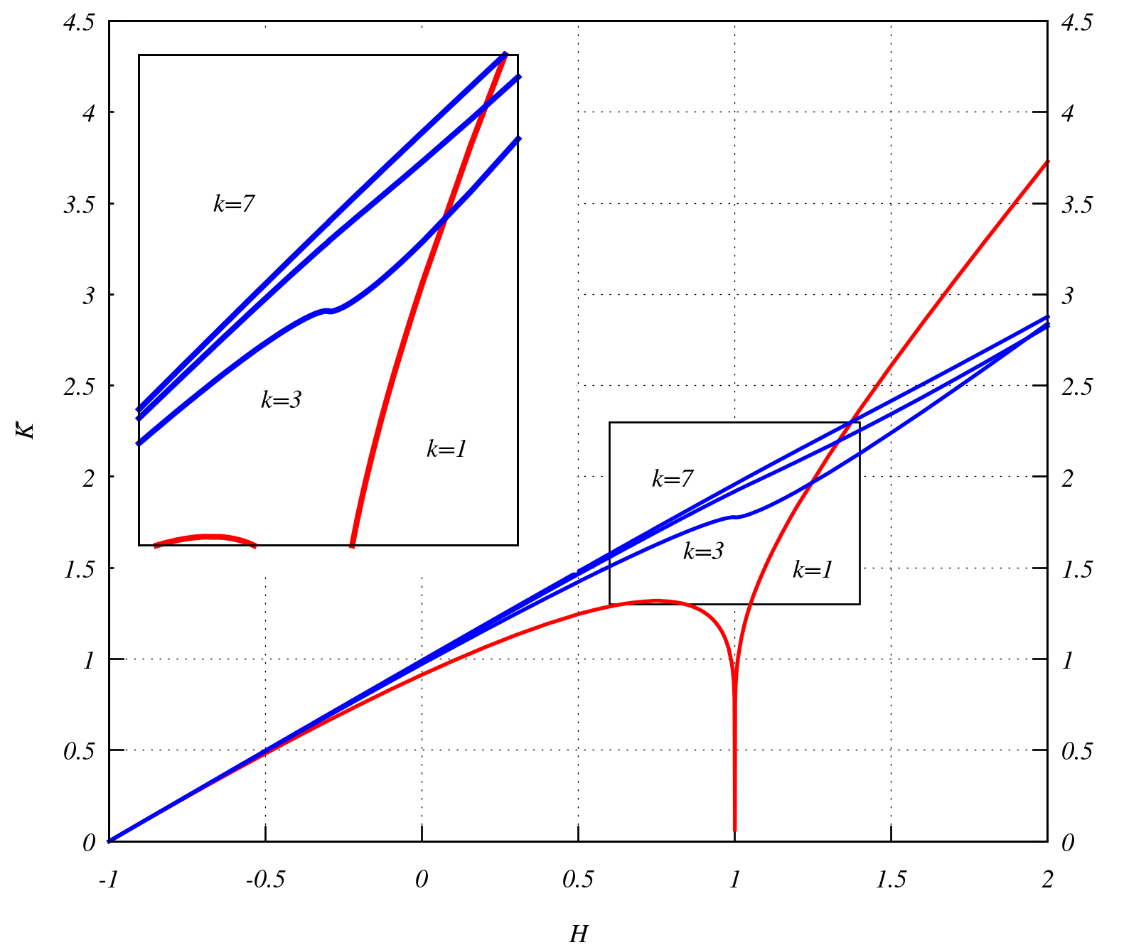
Figure 7. $\tilde{\mathrm{K}}_{k}$, rescaled by $\frac{k+1}{2}$, for the planar pendulum $H=\frac{1}{2}p^{2}-\cos q$ with $k=1,3,5,7$. The inset (upper left) highlights the behaviour near the critical energy level $H=1$.

Let us elaborate on claim 5.3.1. If $H$ is mechanical, $p=H_{p}$, so $\tilde{\mathrm{K}}_{k}=(k+2)^{-1}\times f_{k+2}/f_{k}$. In addition, the change of variables in (eq. 19) implies that for $k\geq 3$, $2\pi f_{k}(I)=k(k-2)H_{I}(I)\times\iint p^{k-3}\mathrm{d}p\wedge\mathrm{d}q$. These two facts imply that $\tilde{\mathrm{K}}_{1}$ tends to $0$ as $I$ approaches a critical action, while $\tilde{\mathrm{K}}_{k}$ tends to a non-zero limit for $k\geq 3$ when the critical action is positive. Figure 7 plots the graphs of $\tilde{\mathrm{K}}_{k}$ for selected values of $k$ and demonstrates these facts for a selected example. In addition, when $H=\frac{1}{2}\left(p^{2}+q^{2}\right)$ is a simple harmonic oscillator, $\tilde{\mathrm{K}}_{k}=\frac{2}{k+1}I$. This fact is seen in figure 7, too.

Figure 6 depicts the level sets of a planar hamiltonian with a saddle cycle $v$ with incoming edges $A$, $B_{0}$ and $B_{1}$ and an outgoing edge $E$ (and there are unique minima inside each white disk-shape region). Case 3 applies to the maximum of both $A$ and $B_{0}$, so the graph of $\tilde{\mathrm{K}}$ on each edge should be roughly $\cap$-shaped. Case 2 applies to the maximum of $B_{1}$ and one expects the graph of $\tilde{\mathrm{K}}$ to be roughly $/$-shaped. Case 3 also applies to the minimum vertex of $E$, so the graph of $\tilde{\mathrm{K}}|_{E}$ should increase monotonically from $0$.

It remains to prove that the vector field $\bar{R}_{0}$ does not have a constant period. The hamiltonian $\overline{G}_{0,\beta}$ of the averaged vector field $\overline{R}_{0}$ and the latter’s hamiltonian $\overline{G}_{0,T}$ with respect to the symplectic form $-T\omega_{\beta}/\overline{G}_{0,\beta}$ from Lemma 4.3 are computed to be

$$\overline{G}_{0,\beta} =(\beta Z(\beta)H_{I}(I))^{-1}\,f(I)\,\tilde{\mathrm{K}}(I)\,\zeta_{l}(\xi)\,\times\exp(-\beta G_{\beta}(I,\xi))$$ (42)

$$\overline{R}_{0} =\dfrac{f(I)\,\tilde{\mathrm{K}}(I)}{H_{I}(I)^{2}}\times\left(-\xi^{l}\,\partial_{I}+\zeta_{l}(\xi)\,H_{I}(I)\,\left[\dfrac{\tilde{\mathrm{K}}(I)-T}{\tilde{\mathrm{K}}(I)}\right]\,\partial_{\xi}\right)$$ (43)

$$\overline{G}_{0,T} =\mathrm{Z}_{l}(\xi)+H(I)-T\ln F_{k}(I),$$ (44)

where $\mathrm{Z}_{l}(\xi)=\frac{1}{2}\xi^{2}-T\ln(\zeta_{l}(\xi)/\zeta_{l}(0))$ and $F=F_{k}$ is defined in (eq. 38). One checks that $\mathrm{Z}_{1}(\xi)=\frac{1}{2}\xi^{2}$ and $F_{1}(I)=I$, so (eq. 44) reproduces the hamiltonian in (eq. 22).

Let it be noted that $(I,\xi)$ are not Darboux coordinates for the rescaled symplectic form. One defines Darboux coordinates via

$$\sigma =\int_{I_{0}}^{I}\frac{(H_{I})^{2}}{f(I)\,\tilde{\mathrm{K}}(I)}\,\mathrm{d}I=\int_{H_{0}}^{H}\mathrm{d}H/F, \chi =\int_{0}^{\xi}\frac{\mathrm{d}\xi}{\zeta_{l}(\xi)}$$ (45)

which for $k=1,l=1$ specializes to the Darboux coordinates introduced above for the Hoover thermostat.

Lemma 5.4.

Let $H:T^{*}\Sigma\longrightarrow{\bf R}$ be a well-behaved, smooth hamiltonian. Then for all $T\in\tau_{H}$, the Watanabe-Kobayashi thermostat (eq. 36) is a separable thermostat in the sense of definition 5.1. In addition, if $l>1$, then conditions 1–3 of Theorem 5.1 are satisfied.

Proof.

Lemma 5.3 proved that condition 2 of the definition of a separable thermostat is satisfied when $T\in\tau_{H}$. It is clear that the other conditions of definition 5.1 hold on the same interval from that lemma.

Let now $T\in\tau_{H}$ and let $H_{0}$ (resp. $I_{0}$) be the energy (resp. action) at the thermostatic equilibrium on the above-mentioned interval. Condition 1 holds by inspection of (eq. 36), and condition 2 holds in view of lemma 5.3. It remains to verify the non-constancy of the period of $\overline{R}_{0}$.

The proof of lemma 5.3 shows that $\tilde{\mathrm{K}}-T$ is negative (resp. positive) on an interval to the left (resp. right) of $I_{0}$. This implies that near $I_{0}$ the graph of the “potential” $U_{T}(I)$ is $\cup$-shaped modulo possible bad behaviour near in a neighbourhood of $I_{0}$ itself. This implies that $\overline{G}_{0,T}$ is proper in some neighbourhood of $(I_{0},0)$.

On the other hand, the hessian of $\overline{G}_{0,T}$

$$\operatorname{hess}\overline{G}_{0,T}=\zeta_{l}(\xi)^{-1}\,\xi^{l-1}(l-\beta\xi^{l+1})\,\left(\mathrm{d}\xi\right)^{2}+T\,\tilde{\mathrm{K}}^{-2}\,\tilde{\mathrm{K}}^{\prime}\,\left(\mathrm{d}H\right)^{2}.$$ (46)

If $\tilde{\mathrm{K}}^{\prime}\neq 0$ at $I_{0}$, then the hessian is positive definite at the thermostatic equilibrium when $l=1$; otherwise it is degenerate. The lowest order term in the coefficient on $(\mathrm{d}\xi)^{2}$ is of degree $l-1$ in $\xi$ since $\zeta_{l}(0)=(2T)^{n}\,n!$. This implies that for $l>1$, $\overline{G}_{0,T}=((2T)^{n}\,n!)^{-1}\,(l+1)^{-1}\,\xi^{l+1}+\frac{1}{2}T^{-1}\,\tilde{\mathrm{K}}^{\prime}(H_{0})\,(H-H_{0})^{2}+O(\xi^{l+3},(H-H_{0})^{3})$. Since $l$ is odd, $\overline{G}_{0,T}$ is proper in a neighbourhood of its critical point. If $l>1$, then the degeneracy of the hessian of $\overline{G}_{0,T}$ at the critical point implies that $\overline{R}_{0}$ is not conjugate to its linearization at the critical point, and therefore its period is not constant.

If $\tilde{\mathrm{K}}^{\prime}=0$ at $I_{0}$, the hessian is degenerate and the period of $\overline{R}_{0}$ cannot be constant in a neighbourhood of $(I_{0},0)$ for similar reasons.

This proves the second part of the lemma. ∎

One is now in a position to prove the analogue to Theorems 5.2 & 5.3.

Theorem 5.4.

Let $H:T^{*}\Sigma\longrightarrow{\bf R}$ be a well-behaved, real-analytic hamiltonian. Then, for all $T\in\tau_{H}$, the period of $\bar{R}_{0}$ is not constant in a neighbourhood of the critical point $(I_{0},0)$.

Proof.

All cases except $l=1$ and $k\geq 3$ follow from Lemma 5.4 or Theorem 5.2, so assume that $l=1$ and $k\geq 3$.

As in the proof of Theorem 5.2, let $\gamma_{0}\in\Gamma_{H}$ be the connected component of the level set of $H$ where the thermostatic equilibrium $(I_{0},0)$ is attained and let $c_{0}\subset\Gamma_{H}$ be the edge containing $\gamma_{0}$.

If $c_{0}$ has a saddle vertex, then either case 2 or 3 of claim 5.3.1 applies. In both cases, $H$ and $F$ are bounded in a $c_{0}$-neighbourhood of the vertex and hence the potential $U_{T}=H-T\ln F$ (eq. 44) is similarly bounded. This contradicts isochronicity. Thus, if $\bar{R}_{0}$ is isochronous, then $c_{0}$ has no saddle vertex. Hence claim 5.2.1 holds.

To prove claim 5.2.2 holds here, one computes, in the Darboux coordinates $(\sigma,\xi)$ (eq. 45), that

$$U_{\sigma}=I_{H}\,f\,\left(\tilde{\mathrm{K}}-T\right)=F_{H}\,\left(\tilde{\mathrm{K}}-T\right).$$ (47)

Assume that the local minimum vertex $\min c_{0}$ is non-degenerate. Then $I_{H}\longrightarrow\omega^{-2}>0$ as $\gamma\searrow\min c_{0}$. On the other hand, both $f$ and $\tilde{\mathrm{K}}$ approach $0$ as $\gamma\searrow\min c_{0}$. This implies that $U_{\sigma}\nearrow 0$ and so $U_{\sigma}$ is bounded on $(\min c_{0},\gamma_{0}]\subset c_{0}$. By the same argument as in the second paragraph following claim 5.2.2, one obtains a contradiction with isochronicity, thereby proving that claim here. Therefore, the local minimum vertex cannot be non-degenerate if the vector field $\bar{R}_{0}$ is isochronous. This completes the proof. ∎

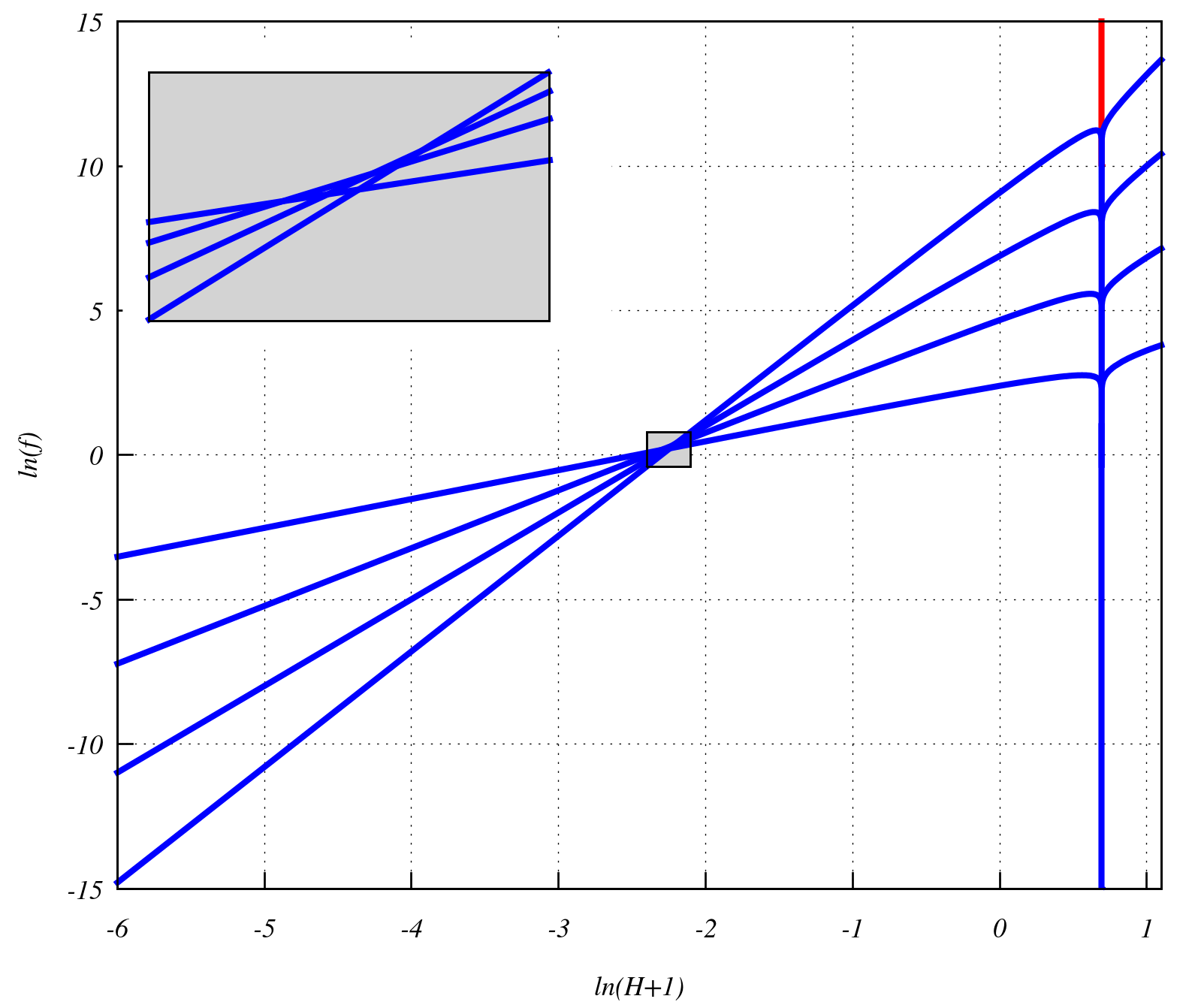
Figure 8. $\ln(f_{k})$ vs. $\ln(H+1)$ for the planar pendulum $H=\frac{1}{2}p^{2}-\cos q$ with $k=3,5,7,9$. The inset (upper left) highlights the behaviour near crossings. The approximate linearity to the left of $H=0$ is striking.

5.5. Hoover & Sprott and Hoover, Sprott & Hoover

In [14], Hoover, Sprott and Hoover obtain numerical results that indicate for some parameter values there are large sets with positive Lyapunov exponents for the thermostat with

$$G_{\beta} =H+\frac{1}{4}\xi^{4}, A_{0} =q, A_{1} =-\xi^{3},$$ (48)

$$B_{0} =p^{3}, B_{1} =-\mu\xi^{3}, C_{1} =1, C_{0} =\left[qH_{q}-T\right]+\mu p^{2}\left[pH_{p}-3T\right].$$

For comparison with [14, eq. [HS],p. 237], their $\xi^{4}$ term is not multiplied by $\beta$ and their $T$ (resp. $\beta$, $\alpha/T$) is $T$ (resp. $\epsilon$, $\epsilon\mu$) here. It is trivial to see that conditions 1, 3 and 4 of definition 5.1 are satisfied. To prove that condition 2 holds, note that on averaging $C_{0}$, one obtains

$$\overline{C}_{0}=\left[\mathrm{K}(I)-T\right]+\mu f(I)\left[\tilde{\mathrm{K}}(I)-T\right],$$ (49)

where $\mathrm{K}$ is the averaged temperature from (eq. 19), $\tilde{\mathrm{K}}=\tilde{\mathrm{K}}_{3}$ is the weighted average temperature from (eq. 37) with $k=3$ and $f=f_{3}$ is defined likewise.

The hamiltonian $\overline{G}_{0,\beta}$ of the averaged vector field $\overline{R}_{0}$ and the latter’s hamiltonian $\overline{G}_{0,T}$ with respect to the symplectic form $-T\omega_{\beta}/\overline{G}_{0,\beta}$ from Lemma 4.3 are computed to be

$$\overline{G}_{0,\beta} =(\beta Z(\beta)H_{I}(I))^{-1}\,\left(\mathrm{K}(I)+\mu f(I)\,\tilde{\mathrm{K}}\right)\exp(-\beta G_{\beta}(I,\xi))$$ (50)

$$\overline{R}_{0} =\frac{1}{H_{I}}\times\left(-\xi^{3}\,(H_{I})^{-1}\,\left[\mathrm{K}(I)+\mu f(I)\,\tilde{\mathrm{K}}(I)\right]\,\partial_{I}+\overline{C}_{0}\,\partial_{\xi}\right)$$ (51)

$$\overline{G}_{0,T} =\xi^{4}/4+\underbrace{H(I)-T\ln Q_{\mu}(I)}_{U_{T}},$$ (52)

where $\ln Q_{\mu}=\int^{H}_{H_{0}}\mathrm{d}H\,\left[\frac{1+\mu f}{\mathrm{K}+\mu f\tilde{\mathrm{K}}}\right]$. One checks that for $\mu=0$ (eq. 52) reproduces the hamiltonian in (eq. 22), while for $\mu=\infty$, the potential coincides with that in (eq. 44).

Lemma 5.5.

Let $H:T^{*}\Sigma\longrightarrow{\bf R}$ be a well-behaved, smooth hamiltonian. Then, for all $T,\mu>0$, the thermostat $\mathrm{T}$ (eq. 48) is a separable thermostat in the sense of definition 5.1.

The proof is similar to that of 5.1.

The following is an immediate consequence of the preceding lemma and the fact that $\overline{G}_{0,T}$ is quartic in $\xi$.

Theorem 5.5.

Let $H:T^{*}\Sigma\longrightarrow{\bf R}$ be a well-behaved, smooth hamiltonian. Then the period of $\bar{R}_{0}$ is not constant in a neighbourhood of the critical point $(I_{0},0)$.

References

- [1] M. Abramowitz and I. A. Stegun, editors. Handbook of mathematical functions with formulas, graphs, and mathematical tables. Dover Publications Inc., New York, 1992. Reprint of the 1972 edition.
- [2] H. C. Andersen. Molecular dynamics simulations at constant pressure and/or temperature. J. Chem. Phys., 72:2384–2393, 1980.
- [3] V. I. Arnol′ d. Mathematical methods of classical mechanics, volume 60 of Graduate Texts in Mathematics. Springer-Verlag, New York, second edition, 1989. Translated from the Russian by K. Vogtmann and A. Weinstein.
- [4] V. I. Arnol′d. Small denominators and problems of stability of motion in classical and celestial mechanics. Uspehi Mat. Nauk, 18(6 (114)):91–192, 1963.
- [5] A. Bolsinov and A. Fomenko. Exact topological classification of hamiltonian flows on smooth two-dimensional surfaces. Journal of Mathematical Sciences, 94(4):1457,1476, 1999.
- [6] A. V. Bolsinov and A. T. Fomenko. Integrable Hamiltonian systems. Chapman & Hall/CRC, Boca Raton, FL, 2004. Geometry, topology, classification, Translated from the 1999 Russian original.
- [7] Butler, Leo T. Topology and integrability in lagrangian mechanics. In H. Canbolat, editor, Lagrangian Mechanics, pages 43–66. Intech, 2016.
- [8] L. Chierchia and G. Pinzari. Properly-degenerate KAM theory (following V. I. Arnold). Discrete Contin. Dyn. Syst. Ser. S, 3(4):545–578, 2010.
- [9] L. Chierchia and G. Pinzari. The planetary -body problem: symplectic foliation, reductions and invariant tori. Invent. Math., 186(1):1–77, 2011.
- [10] L. Chierchia and F. Pusateri. Analytic Lagrangian tori for the planetary many-body problem. Ergodic Theory Dynam. Systems, 29(3):849–873, 2009.
- [11] J. Féjoz. Démonstration du ‘théorème d’Arnold’ sur la stabilité du système planétaire (d’après Herman). Ergodic Theory Dynam. Systems, 24(5):1521–1582, 2004.
- [12] W. G. Hoover. Canonical dynamics: equilibrium phase space distributions. Phys. Rev. A., 31:1695–1697, 1985.
- [13] W. G. Hoover and C. G. Hoover. Singly-Thermostated Ergodicity in Gibbs’ Canonical Ensemble and the 2016 Ian Snook Prize Award. CMST, 23(1):5–8, 2017.
- [14] W. G. Hoover, J. C. Sprott, and C. G. Hoover. Ergodicity of a singly-thermostated harmonic oscillator. Communications in Nonlinear Science and Numerical Simulation, 32(Supplement C):234 – 240, 2016.
- [15] L. D. Landau and E. M. Lifshitz. Mechanics. Course of Theoretical Physics, Vol. 1. Translated from the Russian by J. B. Bell. Pergamon Press, Oxford-London-New York-Paris; Addison-Wesley Publishing Co., Inc., Reading, Mass., 1960.
- [16] F. Legoll, M. Luskin, and R. Moeckel. Non-ergodicity of the Nosé-Hoover thermostatted harmonic oscillator. Arch. Ration. Mech. Anal., 184(3):449–463, 2007.
- [17] F. Legoll, M. Luskin, and R. Moeckel. Non-ergodicity of Nosé-Hoover dynamics. Nonlinearity, 22(7):1673–1694, 2009.
- [18] J. Moser. On the volume elements on a manifold. Transactions of the American Mathematical Society, 120(2):286,294, 1965.
- [19] J. Moser. Stable and random motions in dynamical systems. Princeton Landmarks in Mathematics. Princeton University Press, Princeton, NJ, 2001. With special emphasis on celestial mechanics, Reprint of the 1973 original, With a foreword by Philip J. Holmes.
- [20] A. I. Neishtadt and Y. G. Sinai. Adiabatic piston as a dynamical system. Journal of Statistical Physics, 116(1):815–820, Aug 2004.
- [21] S. Nosé. A unified formulation of the constant temperature molecular dynamics method. J. Chem. Phys., 81:511–519, 1984.
- [22] J. D. Ramshaw. General formalism for singly thermostated hamiltonian dynamics. Phys. Rev. E, 92:052138, Nov 2015.
- [23] S. V. Bolotin and R. S. MacKay. Isochronous potentials. In L. Vázquez, R. S. MacKay, and M. P. Zorzano, editors, Localization And Energy Transfer In Nonlinear Systems, Proceedings Of The Third Conference., pages 217–224. World Scientific, 2003.
- [24] J. A. Sanders, F. Verhulst, and J. Murdock. Averaging methods in nonlinear dynamical systems, volume 59 of Applied Mathematical Sciences. Springer, New York, second edition, 2007.
- [25] K. Shah, D. Turaev, V. Gelfreich, and V. Rom-Kedar. Equilibration of energy in slow–fast systems. Proceedings of the National Academy of Sciences, 114(49):E10514–E10523, 2017.
- [26] D. Tapias, A. Bravetti, and D. P. Sanders. Ergodicity of one-dimensional systems coupled to the logistic thermostat. CMST, 23, 11 2016.
- [27] H. Watanabe and H. Kobayashi. Ergodicity of a thermostat family of the Nosé-Hoover type. Phys. Rev. E, 75:040102, Apr 2007.
- [28] P. Wright. The periodic oscillation of an adiabatic piston in two or three dimensions. Communications in Mathematical Physics, 275(2):553–580, Oct 2007.