Weighted Extended B-Spline Finite Element Analysis of a coupled system of general Elliptic equations

Abstract

In this study we establish the existence and uniqueness of the solution of a coupled system of general elliptic equations with anisotropic diffusion , non-uniform advection and variably influencing reaction terms on Lipschitz continuous domain $\Omega\subset\mathbb{R}^{m}$ (m$\geq$1) with a Dirichlet boundary. Later we consider the finite element (FE) approximation of the coupled equations in a meshless framework based on weighted extended B-Spine functions (WEBS).The a priori error estimates corresponding to the finite element analysis are derived to establish the convergence of the corresponding FE scheme and the numerical methodology has been tested on few examples.

1 Introduction

In this paper we are considering the following class of coupled system,namely general elliptic equations, related to the advection-reaction-diffusion systems appearing in the chemical and biological phenomena:

$$\left\{\begin{array}[]{ll}-\nabla.(\mathfrak{P}(\nabla u_{1})^{\prime})+\mathfrak{R}.\nabla u_{1}+q_{1}u_{1}+q_{2}u_{2}=f_{1},~{}~{}in~{}\Omega\\ -\nabla.(\mathfrak{P}(\nabla u_{2})^{\prime})+\mathfrak{R}.\nabla u_{2}+q_{1}u_{2}-q_{2}u_{1}=f_{2},~{}~{}in~{}\Omega\end{array}\right.$$ (3)

subjected to the Dirichlet boundary condition , where $\Omega$ is a Lipschitz continuous bounded domain in $\mathbb{R}^{m}$ and the functions $q_{1}$ , $q_{2}$ are real essentially bounded which, in order to simplify the exposition,are assumed through out this paper to satisfy certain conditions (see section 3).$\mathfrak{P}$ and $\mathfrak{R}$ are $m\times m$ symmetric matrix and $m\times 1$ vector of essential bounded functions respectively.The elliptic system (3) represents a steady case of reaction-diffusion system of interest in mathematical biology and physicssweers2003bifurcation .Here real functions $u_{1},u_{2}$ which are called activator and inhibitor respectively, can be interpreted as relative concentrations of two substances known as morphogens and the functions $\Phi_{1},\Phi_{2}$ models autocatalytic and saturation effects.In the recent years,a lot of research has been focused on the reaction-diffusion system (3) with cross-diffusion ,electrochemical engineering problem, from theoretical and numerical aspects, and among them coupled system of elliptic equations have received considerable attention,various forms of this system have been proposed in the literature. The aim of this paper is to obtain an existence and uniqueness of the solutions on any bounded Lipschitz domain, in addition to carry out a new meshless (WEB-S) numerical method for the approximate solutions of the system.
On an arbitrary domain finite element approximation of these equations is a highly sought after approach to obtain their numerical solution;In particular WEB-FEM combines the computational advantages of B-Splines and standard mesh-based finite elements.Further it attains the degree and smoothness to be chosen flexibly without substantially increasing the size of problem.Off late spectral Galerkin method chen2015new , Lattice-Boltzmann schemes suga2009stability etc have been used for numerical approximations.In boglaev2012numerical Boglaev have used method of upper and lower solutions , and construct monotone sequence for difference scheme to approximate the solution of coupled system and Xiu et.al chen2015local used stochastic Galerkin and stochastic collocation method in conjunction with the gPC expansions. In view of the computational advantages WEBS-FEA is one of highly desired approach to solve the coupled elliptic system.In the current literature no work is reported on WEBS-FEA of the general coupled elliptic problem.

Weighted Extended B-splines are a new class of finite element basis functions on a conventional cartesian grid of nearly zero cost for solving Dirichlet problems on bounded domains in arbitrary dimensions.It was first proposed by Hollig et al. in hollig2001weighted -hollig2003nonuniform . The WEB-FEM does not require any grid generation. Because of the simple subdivision formulas for tensor product B-splines, grid refinement techniques are easily implemented. The WEB-FEM is a meshless technique which combines the computational efficiency of B-splines and standard mesh-based elements,with weight functions taking care of the boundary.

Here the finite elements are constructed with scaled translates $b^{n}_{k}$,k $\in$ $\mathbb{Z}^{m}$ of the standard m-variate tensor product B-spline of order n. B-splines $b^{n}_{k}$ ($b_{k}$ in abbrev) are polynomials of degree n-1 in the variables $x_{1},x_{2},x_{3}.....x_{m}$ on each grid cells $\mathbb{Q}_{l}$ = h ($[0,1]^{m}$ + $l$), $k_{i}\leq l_{i}\leq k_{i}+n$ in their support(see figure (1) ; provided by H$\ddot{o}$llig).In case of Dirichlet problem on a bounded domain $\Omega\subset\mathbb{R}^{m}$, we multiply $b_{k}$ by a smoothed version w of the distance function to $\partial\Omega$. Then the span of weighted B-splines

$$span\{wb_{k}:\Omega\cap supp~{}b_{k}\neq\phi\}$$

is a possible finite element subspace which conforms both the boundary conditions and yields approximations of optimal order.

In our forthcoming discussion bold letters represents a vector field (i.e, vector valued functions). Henceforth , the grid width used for the spline approximation is denoted by h, and for the functions f,g we write f $\preceq$ g , if f $\leq$ cg and f $\asymp$ g ,if f=cg for some positive constant c which doesn’t depend on the grid width , indices, or arguments of functions and if $\mathbf{x}=(x_{1},x_{2}),\mathbf{y}=(y_{1},y_{2})$ then $\mathbf{x}\star\mathbf{y}=(x_{1}y_{1},x_{2}y_{2})$

The paper is organized under six sections. Abstract variational formulation of the problem is introduced in section (2). Section (3) deals with the existence and uniqueness aspects of the problem. Section (4) deals with a priori estimates and the convergence analysis. Numerical examples are presented in section (5)

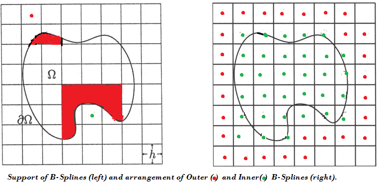
Figure 1: Outer and Inner b-splines

2 Abstract Variational Formulation

Let us consider an abstract boundary value problem

$$\mathcal{L}\mathbf{u}=\mathbf{f},~{}~{}in~{}\Omega~{}~{}and\mathcal{B}\mathbf{u}=0~{}on~{}\partial\Omega$$

with a differential operator $\mathcal{L}$ and an operator $\mathcal{B}$ describing the boundary conditions. Moreover, this problem admits a variational formulation ,(see brenner2008mathematical )

$$a(\mathbf{u,v})=\lambda(\mathbf{v}),~{}~{}\mathbf{v}~{}\in H$$ (4)

where $a$ is a bilinear form and $\lambda$ is a linear functional on a Hilbert Space $H$.Then, for a finite element subspace $\mathbb{B}_{h}\subset H$, the Ritz-Galerkin approximation $\mathbf{u}_{h}$ is defined by

$$a(\mathbf{u}_{h},\mathbf{v}_{h})=\lambda(\mathbf{v}_{h}),~{}\mathbf{v}_{h}~{}\in~{}\mathbb{B}_{h}$$

The coefficients $\mathbf{a}_{i}$ of $\mathbf{u}_{h}$ with respect to a basis $\mathbf{B}_{i}$ of $\mathbb{B}_{h}$ , are determined via the linear system obtained by using $\mathbf{v}_{h}$ = $\mathbf{B}_{k}$ as test functions.

2.1 Ritz-Galerkin Approximation

The Ritz-Galerkin approximation $\mathbf{u}_{h}(\sum_{i}\mathbf{a}_{i}\star\mathbf{B}_{i}$ $\in$ $\mathbb{B}_{h}$ $\subset H$) of the variational problem (4) is determined by the linear system

$$\sum_{i}a(\mathbf{B_{i},B_{k}})=\lambda(\mathbf{B}_{k})$$

$$\textrm{which is written as},$$

$$\mathbf{G}_{h}\mathbf{U=F}.$$

It is well known (cf. gilbarg2015elliptic and strang1973analysis ) that the error of the approximation $\mathbf{u}_{h}$ can be bounded in terms of the distance of u to the subspace $\mathbb{B}_{h}$, spanned by $\mathbf{B}_{i}$.For $\mathbf{v}$ $\in$ $H^{l}(\Omega)$

$$||\mathbf{v}||_{l,\Omega}=\big{(}\sum_{|\alpha|\leq l}\int_{\Omega}|D^{\alpha}\mathbf{v}|^{2}\big{)}^{1/2}$$

represents the norm of the Sobolev space $H^{l}(\Omega)$ we have

$$||\mathbf{u-u_{h}}||_{1}\preceq inf_{\mathbf{v}_{h}\in\mathbb{B}_{h}}||\mathbf{u-v_{h}}||_{1}$$

which in other words implies the following typical error estimate for the standard finite element subspaces involving piecewise polynomials of degree $\leq$ $n-1$

$$||\mathbf{u-u_{h}}||_{1}\preceq h^{n-1}||\mathbf{u}||_{n}$$ (5)

Finally , a feasible estimation for the Galerkin matrix is essential and for standard finite element subspaces using quasi-uniform partitions, the condition with respect to the 2-norm can be bounded in terms of the grid width,

$$cond_{2}G_{h}\preceq h^{-2}$$ (6)

which is moderate enough so that iterative methods, like the preconditioned conjugate gradient algorithm, can be employed to solve the Galerkin system efficiently and in a stable way.We shall show in the following that the properties (5) and (6) remain valid for our new class of finite elements. Hence,WEB-FEM conforms the basic requirements of approximation.

3 Coupled System of General Elliptic Operators

In this section we will study some questions related to the existence and uniqueness of solutions , of the coupled systems of equations of general elliptic operators.

3.1 Existence and uniqueness

Consider the following system of general Elliptic Equations :

$$\left\{\begin{array}[]{ll}-\nabla.(\mathfrak{P}(\nabla u_{1})^{\prime})+\mathfrak{R}.\nabla u_{1}+q_{1}(\mathbf{x})u_{1}+q_{2}(\mathbf{x})u_{2}=f_{1}(\mathbf{x}),~{}~{}in~{}\Omega\\ -\nabla.(\mathfrak{P}(\nabla u_{2})^{\prime})+\mathfrak{R}.\nabla u_{2}+q_{1}(\mathbf{x})u_{2}-q_{2}(\mathbf{x})u_{1}=f_{2}(\mathbf{x}),~{}~{}in~{}\Omega\end{array}\right.$$

with $u_{1}=u_{2}$ = 0 on the boundary, $\mathfrak{P}=(a_{ij}(\mathbf{x}))_{n\times n},$ is a symmetric matrix and $\mathfrak{R}=(r_{k}(\mathbf{x}))_{n\times 1}~{}~{},~{}^{\prime}$ denote transpose. If $f_{1},f_{2},u_{1},u_{2}\in L^{2}(\Omega)$ then from regularity theorem $u_{1},u_{2}~{}\in H^{2}(\Omega)$.Precisely,u $\in(H^{2}(\Omega)\bigcap H^{1}_{0}(\Omega))^{2}$

Let $\Omega$ be a bounded open set in $\mathbb{R}^{n}$. Consider the space $(H_{0}^{1}(\Omega))^{2}=V$ with its product norm($||(._{1},._{2})||=||._{1}||+||._{2}||$). Define for u=($u_{1},u_{2}$), v=($v_{1},v_{2}$) in V, the bilinear form

a(u,v)= $\int_{\Omega}[\nabla v_{1}\mathfrak{P}(\nabla u_{1})^{\prime}+\nabla v_{2}\mathfrak{P}(\nabla u_{2})^{\prime}]+\int_{\Omega}[v_{1}\mathfrak{R}.\nabla u_{1}+v_{2}\mathfrak{R}.\nabla u_{2}]+\int_{\Omega}\textbf{u}\mathfrak{Q}\textbf{v}^{\prime}$

$$where,\mathfrak{Q}=\left(\begin{array}[]{cc}q_{1}&-q_{2}\\ q_{2}&q_{1}\end{array}\right)$$

Clearly,

$$a(\textbf{u},\textbf{u})=\int_{\Omega}[\nabla u_{1}\mathfrak{P}(\nabla u_{1})^{\prime}+\nabla u_{2}\mathfrak{P}(\nabla u_{2})^{\prime}]+\int_{\Omega}[u_{1}\mathfrak{R}.\nabla u_{1}+u_{2}\mathfrak{R}.\nabla u_{2}]+\int_{\Omega}q_{1}(u_{1}^{2}+u_{2}^{2})$$ (7)

which may not be coercive in general. Thus if f = ($f_{1},f_{2}$)  $\in~{}(L^{2}(\Omega))^{2}$, we cannot use Lax-Milgram lemma directly to prove the existence of a solution to the problem: Find u $\in V$ such that

$$a(\textbf{u},\textbf{v})=\langle\textbf{f},\textbf{v}\rangle,for~{}every~{}\mathbf{v}~{}\in V$$ (8)

Theorem 3.1

Let us assume that $\exists$ a $\alpha>$0 such that, $A^{\prime}\mathfrak{P}A\geq\alpha A^{\prime}A$ and ess-inf{$q_{1}(x)$ : $x\in\Omega$}=$\kappa\geq\frac{\alpha}{2}+\frac{\mathcal{B}^{2}}{2\alpha}$ a.e in $\Omega$ where, $\mathcal{B}^{2}=\Sigma_{1}^{n}\parallel r_{k}\parallel^{2}_{\infty}~{}~{}a_{ij},r_{k},q_{1},q_{2}\in L^{\infty}(\Omega)$ then (8) possess an unique solution.

Proof

We shall proceed as follows. From (7) we obtain,

$$a(\textbf{u,u})\succeq(|u_{1}|^{2}_{H^{1}(\Omega)}+|u_{2}|^{2}_{H^{1}(\Omega)})+\int_{\Omega}\sum_{k}r_{k}(x)[\frac{\partial u_{1}}{\partial x_{k}}u_{1}+\frac{\partial u_{2}}{\partial x_{k}}u_{2}]+\int_{\Omega}q_{1}(u_{1}^{2}+u_{2}^{2})$$

Estimation from H$\ddot{o}$lder’s Inequality,

$$|\int_{\Omega}\sum_{k}r_{k}(x)\frac{\partial u_{1}}{\partial x_{k}}u_{1}|$$ (9)

$$\leq \int_{\Omega}\Sigma_{k}|r_{k}(x)||\frac{\partial u_{1}(x)}{\partial x_{k}}||u_{1}|$$

$$\leq \Sigma_{k}||r_{k}||_{L^{\infty}(\Omega)}\int_{\Omega}|\frac{\partial u_{1}(x)}{\partial x_{k}}||u_{1}|$$

$$\leq \Sigma_{k}||r_{k}||_{L^{\infty}(\Omega)}||\frac{\partial u_{1}}{\partial x_{k}}||_{L^{2}(\Omega)}||u_{1}||_{L^{2}(\Omega)}$$

$$\leq \mathcal{B}|u_{1}|_{H^{1}(\Omega)}||u_{1}||_{L^{2}(\Omega)}$$

Similarly,

$$|\int_{\Omega}\sum_{k}r_{k}(x)\frac{\partial u_{2}}{\partial x_{k}}u_{2}|\leq\mathcal{B}|u_{2}|_{H^{1}(\Omega)}||u_{2}||_{L^{2}(\Omega)}$$

Therefore,

$$a(\textbf{u,u})\succeq(|u_{1}|^{2}_{H^{1}(\Omega)}+|u_{2}|^{2}_{H^{1}(\Omega)})-\mathcal{B}(|u_{1}|_{H^{1}(\Omega)}||u_{1}||_{L^{2}(\Omega)}+|u_{2}|_{H^{1}(\Omega)}$$

$$+||u_{2}||_{L^{2}(\Omega)})+\kappa(||u_{1}||^{2}_{L^{2}(\Omega)}+||u_{2}||^{2}_{L^{2}(\Omega)})$$ (10)

from the inequality, $ab\leq\frac{\delta a^{2}}{2}+\frac{b^{2}}{2\delta}$ finally we obtain ,

$$a(\textbf{u,u})\succeq(||u_{1}||_{H^{1}(\Omega)}^{2}+||u_{2}||_{H^{1}(\Omega)}^{2})\succeq||\mathbf{u}||^{2}_{V},~{}~{}i.e~{}coercive$$ (11)

Moreover from Poincare and C-S Inequality it can be shown that,

$$a(\textbf{u,v})\preceq||\mathbf{u}||_{V}||\mathbf{v}||_{V},~{}~{}i.e~{}continuous$$ (12)

Hence,Lax-Milgram lemma ensures a unique solution of (8)

Definition 3.1

Weighted Extended B-Splines [WEB-S]

For i $\in$ I, the WEB-S $B_{i}$ is defined by

$$B_{i}=\frac{w}{w(x_{i})}\Big{(}b_{i}+\sum\limits_{j\in{J}}e_{i,j}b_{j}\Big{)},$$

where $x_{i}$ denotes the center of the grid cell $\mathbb{Q}_{i+l(i)}$ corresponding $b_{i}$.The coefficients $e_{i,j}$ satisfy

$$|e_{i,j}|\preceq 1,e_{i,j}=0for||i-j||\succeq 1$$

and are chosen so that all weighted polynomials ( abbrev wp) of order n are contained in the web space $\mathbb{B}_{h}=span\{B_{i}:i\in\mathbf{I}$}

4 Convergence of WEB-Spline

In this section we prove that the numerical solution [$u_{1,h},u_{2,h}$] converges to a weak solution [$u_{1},u_{2}$] as h $\rightarrow$ 0. Moreover we have extended all our preceding results in vector field.

4.1 Error Estiamtion

Theorem 4.1

Assume $\mathbf{u}\in H_{0}^{n}(\Omega)$ is the solution of (8) and $\mathbf{u}_{h}$ is the solution of discrete system of (3) , then the following error estimation holds :

$$|\mathbf{u-u_{h}}|_{1}\preceq h^{n-1}||\mathbf{u}||_{n}$$

Proof

Let, $\mathbf{u_{h}}=(u_{1,h},u_{2,h})$ be the discrete and $\mathbf{u}=(u_{1},u_{2})$ be a weak solution of the system (3). Then we have the following error equations.

$$\left\{\begin{array}[]{ll}\int_{\Omega}\nabla v_{1}\mathfrak{P}[\nabla(u_{1}-u_{1,h})]^{\prime}+\int_{\Omega}\mathfrak{R}.\nabla(u_{1}-u_{1,h})v_{1}+\int_{\Omega}q_{1}(u_{1}-u_{1,h})v_{1}+\int_{\Omega}q_{2}(u_{2}-u_{2,h})v_{1}=0\\ \int_{\Omega}\nabla v_{2}\mathfrak{P}[\nabla(u_{2}-u_{2,h})]^{\prime}+\int_{\Omega}\mathfrak{R}.\nabla(u_{2}-u_{2,h})v_{2}+\int_{\Omega}q_{1}(u_{2}-u_{2,h})v_{2}-\int_{\Omega}q_{2}(u_{1}-u_{1,h})v_{2}=0\end{array}\right.$$

for all $\mathbf{v}=(v_{1},v_{2})$ $\in$ V

taking $(u_{1,h}-\mathrm{P_{h}}u_{1},u_{2,h}-\mathrm{P_{h}}u_{2})$ as a test function to the above discrete error equation, we have the equality.

$$\int_{\Omega}\nabla(u_{1,h}-\mathrm{P_{h}}u_{1})\mathfrak{P}[\nabla(u_{1}-u_{1,h})]^{\prime}+\int_{\Omega}\mathfrak{R}.\nabla(u_{1}-u_{1,h})(u_{1,h}-\mathrm{P_{h}}u_{1})$$

$$+\int_{\Omega}q_{1}(u_{1}-u_{1,h})(u_{1,h}-\mathrm{P_{h}}u_{1})+\int_{\Omega}q_{2}(u_{2}-u_{2,h})(u_{1,h}-\mathrm{P_{h}}u_{1})=0$$ (13)

$$\int_{\Omega}\nabla(u_{2,h}-\mathrm{P_{h}}u_{2})\mathfrak{P}[\nabla(u_{2}-u_{2,h})]^{\prime}+\int_{\Omega}\mathfrak{R}.\nabla(u_{2}-u_{2,h})(u_{2,h}-\mathrm{P_{h}}u_{2})$$

$$+\int_{\Omega}q_{1}(u_{2}-u_{2,h})(u_{2,h}-\mathrm{P_{h}}u_{2})-\int_{\Omega}q_{2}(u_{1}-u_{1,h})(u_{2,h}-\mathrm{P_{h}}u_{2})=0$$ (14)

from (13),

$$\int_{\Omega}\sum_{i,j}a_{ij}\frac{\partial}{\partial x_{i}}(u_{1}-u_{1,h})\frac{\partial}{\partial x_{j}}(u_{1}-u_{1,h}) = \int_{\Omega}\sum_{i,j}a_{ij}\frac{\partial}{\partial x_{i}}(u_{1}-u_{1,h})\frac{\partial}{\partial x_{j}}(u_{1}-\mathrm{P_{h}}u_{1})$$

$$+\int_{\Omega}\mathfrak{R}.\nabla(u_{1}-u_{1,h})(u_{1,h}-\mathrm{P_{h}}u_{1}) - \int_{\Omega}q_{1}(u_{1}-u_{1,h})^{2}$$

$$+\int_{\Omega}q_{1}(u_{1}-u_{1,h})(u_{1}-\mathrm{P_{h}}u_{1}) - \int_{\Omega}q_{2}(u_{2}-u_{2,h})(u_{1}-u_{1,h})+\int_{\Omega}q_{2}(u_{2}-u_{2,h})(u_{1}-\mathrm{P_{h}}u_{1})$$

Similarly (14) yields,

$$\int_{\Omega}\sum_{i,j}a_{ij}\frac{\partial}{\partial x_{i}}(u_{2}-u_{2,h})\frac{\partial}{\partial x_{j}}(u_{2}-u_{2,h}) = \int_{\Omega}\sum_{i,j}a_{ij}\frac{\partial}{\partial x_{i}}(u_{2}-u_{2,h})\frac{\partial}{\partial x_{j}}(u_{2}-\mathrm{P_{h}}u_{2})$$

$$+\int_{\Omega}\mathfrak{R}.\nabla(u_{2}-u_{2,h})(u_{2,h}-\mathrm{P_{h}}u_{2}) - \int_{\Omega}q_{1}(u_{2}-u_{2,h})^{2}$$

$$+\int_{\Omega}q_{1}(u_{2}-u_{2,h})(u_{2}-\mathrm{P_{h}}u_{2}) + \int_{\Omega}q_{2}(u_{1}-u_{1,h})(u_{2}-u_{2,h})-\int_{\Omega}q_{2}(u_{1}-u_{1,h})(u_{2}-\mathrm{P_{h}}u_{2})$$

adding both,

$$\int_{\Omega}\sum_{i,j}a_{ij}[\frac{\partial}{\partial x_{i}}(u_{2}-u_{2,h})\frac{\partial}{\partial x_{j}}(u_{2}-u_{2,h})+\frac{\partial}{\partial x_{i}}(u_{1}-u_{1,h})\frac{\partial}{\partial x_{j}}(u_{1}-u_{1,h})]$$

$$=\int_{\Omega}\sum_{i,j}a_{ij}[\frac{\partial}{\partial x_{i}}(u_{2}-u_{2,h})\frac{\partial}{\partial x_{j}}(u_{2}-\mathrm{P_{h}}u_{2})+\frac{\partial}{\partial x_{i}}(u_{1}-u_{1,h})\frac{\partial}{\partial x_{j}}(u_{1}-\mathrm{P_{h}}u_{1})]$$

$$-\int_{\Omega}q_{2}[(u_{1}-u_{1,h})(u_{2}-\mathrm{P_{h}}u_{2})-(u_{2}-u_{2,h})(u_{1}-\mathrm{P_{h}}u_{1})]-\int_{\Omega}q_{1}[(u_{1}-u_{1,h})^{2}+(u_{2}-u_{2,h})^{2}]$$

$$+\int_{\Omega}q_{1}[(u_{1}-u_{1,h})(u_{1}-\mathrm{P_{h}}u_{1})+(u_{2}-u_{2,h})(u_{2}-\mathrm{P_{h}}u_{2})]$$

from our assumption , $\mathfrak{P}$ is positive definite by $\alpha~{}>$ 0 and $a_{ij}~{}\in~{}L^{\infty}$ yields ,

$$\alpha\int_{\Omega}\sum_{i}[|\frac{\partial}{\partial x_{i}}(u_{2}-u_{2,h})|^{2}+|\frac{\partial}{\partial x_{i}}(u_{1}-u_{1,h})|^{2}]\preceq|u_{1}-u_{1,h}|_{1}|u_{1}-\mathrm{P_{h}}u_{1}|_{1}+|u_{2}-u_{2,h}|_{1}|u_{2}-\mathrm{P_{h}}u_{2}|_{1}$$

$$+|u_{1}-u_{1,h}|_{0}(|u_{2}-\mathrm{P_{h}}u_{2}|_{0}+|u_{1}-\mathrm{P_{h}}u_{1}|_{0})+|u_{2}-u_{2,h}|_{0}(|u_{1}-\mathrm{P_{h}}u_{1}|_{0}$$

$$+|u_{2}-\mathrm{P_{h}}u_{2}|_{0})-\int_{\Omega}q_{1}[(u_{1}-u_{1,h})^{2}+(u_{2}-u_{2,h})^{2}]$$

$$\int_{\Omega}q_{1}[(u_{1}-u_{1,h})^{2}+(u_{2}-u_{2,h})^{2}]+\frac{\alpha}{2}|\mathbf{u-u_{h}}|^{2}_{1}\preceq|\mathbf{u-u_{h}}|_{1}|\mathbf{u-\mathrm{P_{h}}u}|_{1}+|\mathbf{u-u_{h}}|_{0}|\mathbf{u-\mathrm{P_{h}}u}|_{0}$$ (15)

from the inequality , $\frac{(a+b)^{2}}{2}\leq(a^{2}+b^{2})$ and our definition of product norms.

Clearly $q_{1}>0$ , hence

$$|\mathbf{u-u_{h}}|_{1}\preceq|\mathbf{u-\mathrm{P_{h}}u}|_{1};\textrm{from Poincare Inequality}$$ (16)

Now we give the projection error estimate for u,

Theorem 4.2

Let, $\mathbf{u}\in H^{n}$ be a weak solution of .Then,

$$\|\mathbf{u-\mathrm{P_{h}}u}\|_{1}\preceq h^{n-1}\|\mathbf{u}\|_{n}$$ (17)

The proof uses standard quasi interpolation techniques and can be found on hollig2003finite .

Hence from (15) and (17) we obtain

$$|\mathbf{u-u_{h}}|_{1}\preceq h^{n-1}||\mathbf{u}||_{n},~{}~{}if~{}\textbf{u}~{}\in~{}H^{n}_{0}$$

required error estimation of the system (2).

5 Numerical Experiments

In this section we demonstrate a test example belonging to the class of convection-diffusion equations. In the non isothermal chemical reaction process involving chemical species, the chemical concentrations and the temperature are governed by a coupled system of reaction diffusion equations of the form of (3). We present a selected numerical examples concerning our discussions on preceding sections.The domain in our examples is a quadrant circle $\Omega$ = $\{(x,y):x,y\geq$0 and $1-x^{2}-y^{2}\leq 0\}$, and zero boundary conditions are imposed on $\partial\Omega$.Here, n= degree of the polynomial , h= grid width , e = $L_{2}$ error. Corresponding graphs for the solutions , residual error functions (for h=0.1 and highest order of n) and computation time shown in Figures were measured on a Intel Core i7-4770S CPU 3.10 GHz.

For the following problem, the finite element approximation with B-splines requires :

• specification of the functions and constants appearing in the partial differential equations.

• description of the domain and the essential boundary.

• choice of the spline space.

The domain and the essential boundary are represented by weight functions.

5.1 Weight Functions

The domain $\Omega$ is a subset of the unit square described implicitly by a weight function $w_{\Omega}$ :

$$\Omega=\{(x,y)\in(0,1)^{2}:w_{\Omega}(x,y)>0\}$$

The boundary condition u = 0 on the essential part $\Gamma$ of $\partial\Omega$ is incorporated by a weight function w which is of one sign on $\Omega$ and vanishes linearly on $\Gamma$ cf hollig2004finite

$$\Gamma=\{(x,y)\in\partial\Omega:w_{\Omega}(x,y)=0\}$$

5.2 Splines

For all boundary value problems, solutions are approximated by linear combinations of weighted B-splines:

$$\mathbf{u(x,y)}\approx\mathbf{u}_{h}(x,y)=\sum_{k_{1}=1}^{H+n}\sum_{k_{2}=1}^{H+n}\ w(x,y)\mathbf{u}_{k}(x,y)\star\mathbf{b}_{k}(x,y)~{};\hskip 5.69054ptk=(k_{1},k_{2})$$

for (x,y) $\in(0,1)^{2}$ with $w_{\Omega}>$ 0. Here

• h is the grid width.

• n is the degree of the B-Splines.

• the coefficients $\mathbf{u}_{k}$ are vectors

• $b_{k}$ is the uniform tensor product B-Spline with support ,

  $$[(k_{1}-n-1)h,k_{1}h]\times[(k_{2}-n-1)h,k_{2}h]$$

  corresponds to the grid position k = $(k_{1},k_{2})$

5.3 Residual for the partial differential equation

The residual of the Ritz-Galerkin approximation $\mathbf{u}_{h}$ is defined as

$$r(x,y)=(L\mathbf{u}_{h})(x,y)-f(x,y)$$

where , L is the differential operator of the boundary value problem. The relative error

$$e=||r||_{0,\Omega}/||f||_{0,\Omega}$$

with $||.||_{0,\Omega}$ denoting the $L_{2}$ norm on $\Omega$ provides a measure of accuracy for the solution without having to resort to grid refinement,for details hollig2003nonuniform

5.4 Example: BVP with polynomial coefficients

$$-\nabla.((1+x)(1+y)\nabla u_{1})+xu_{1}+xyu_{2}=\frac{x}{10}-\frac{y}{100}$$ (18)

$$-\nabla.((1+x)(1+y)\nabla u_{2})+xu_{2}-xyu_{1}=\frac{x^{2}}{100}$$ (19)

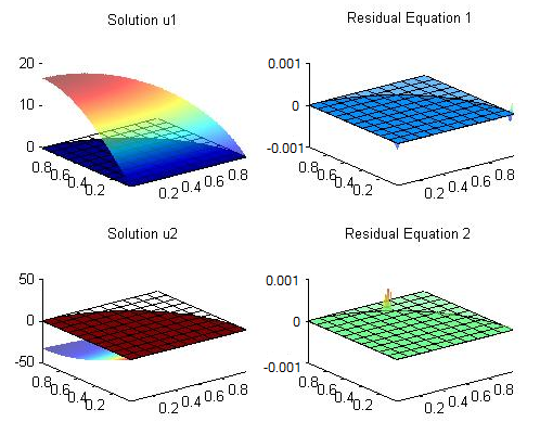
Figure 2: solution functions and the residual error functions corresponding n=4 and h=0.1

6 Conclusion

Following Galerkin Method of Approximation, Existence and Uniqueness of the Non-Cooperative Elliptic Equations has been successfully established.Jackson Inequality, stability estimates of WEB-S basis and Poincare Inequality facilitate the derivation of a priori error estimates to the WEBS-FEA of this system. The proposed WEBS-FE based numerical scheme has been successfully tested on few models.

References

• (1) Sweers, Guido, and William C. Troy. ”On the bifurcation curve for an elliptic system of FitzHugh Nagumo type.” Physica D: Nonlinear Phenomena 177.1-4 (2003): 1-22.
• (2) Chen, Feng. ”A new framework of GPU-accelerated spectral solvers: collocation and Glerkin methods for systems of coupled elliptic equations.” Journal of Scientific Computing 62.2 (2015): 575-600.
• (3) Suga, Shinsuke. ”Stability and accuracy of lattice Boltzmann schemes for anisotropic advection-diffusion equations.” International Journal of Modern Physics C 20.04 (2009): 633-650.
• (4) Boglaev, Igor. ”Numerical solutions of coupled systems of nonlinear elliptic equations.” Numerical Methods for Partial Differential Equations 28.2 (2012): 621-640.
• (5) Chen, Yi, et al. ”Local polynomial chaos expansion for linear differential equations with high dimensional random inputs.” SIAM Journal on Scientific Computing 37.1 (2015): A79-A102.
• (6) H llig, Klaus, Ulrich Reif, and Joachim Wipper. ”Weighted extended B-spline approximation of Dirichlet problems.” SIAM Journal on Numerical Analysis 39.2 (2001): 442-462.
• (7) Hollig, Klaus. Finite element methods with B-splines. Vol. 26. Siam, 2003.
• (8) H llig, Klaus, and Ulrich Reif. ”Nonuniform web-splines.” Computer Aided Geometric Design 20.5 (2003): 277-294.
• (9) Brenner, Susanne, and Ridgway Scott. The mathematical theory of finite element methods. Vol. 15. Springer Science and Business Media, 2007.
• (10) Gilbarg, David, and Neil S. Trudinger. Elliptic partial differential equations of second order. springer, 2015.
• (11) Strang, Gilbert, and George J. Fix. An analysis of the finite element method. Vol. 212. Englewood Cliffs, NJ: Prentice-hall, 1973.