Abstract

Motivated by an explanation of the $R_{K^{(*)}}$ anomalies, we propose a Standard Model extension via two scalar SU(2)_L triplet leptoquarks and three generations of triplet Majorana fermions. The gauge group is reinforced by a $Z_{2}$ symmetry, ensuring the stability of the lightest $Z_{2}$-odd particle, which is a potentially viable dark matter candidate. Neutrino mass generation occurs radiatively (at the three-loop level), and leads to important constraints on the leptoquark couplings to leptons. We consider very generic textures for the flavour structure of the $h_{1}$ leptoquark Yukawa couplings, identifying classes of textures which succeed in saturating the $R_{K^{(*)}}$ anomalies. We subsequently carry a comprehensive analysis of the model’s contributions to numerous high-intensity observables such as meson oscillations and decays, as well as charged lepton flavour violating processes, which put severe constraints on the flavour structure of these leptoquark extensions. Our findings suggest that the most constraining observables are $K^{+}\to\pi^{+}\nu\bar{\nu}$ decays, and charged lepton flavour violating $\mu-e$ conversion in nuclei (among others). Nevertheless, for several classes of flavour textures and for wide mass regimes of the new mediators (within collider reach), this Standard Model extension successfully addresses neutrino mass generation, explains the current $R_{K^{(*)}}$ tensions, and offers a viable dark matter candidate.

1 Introduction

Despite the many successes of the Standard Model (SM) in interpreting experimental data and predicting new phenomena, three independent observations signal the need to consider New Physics (NP) scenarios: neutrino oscillations, the baryon asymmetry of the Universe (BAU), and the lack of a viable dark matter (DM) candidate. Although no direct evidence for NP states has been unveiled at the LHC, certain experimental measurements have revealed non-negligible tensions with respect to the SM predictions. In addition to the anomalous magnetic moment of the muon, recent data hints to several discrepancies with respect to the SM in some $B$-meson decay modes, potentially suggesting the violation of lepton flavour universality (LFUV). In the SM’s original formulation, gauge interactions (both charged and neutral currents) are strictly lepton flavour universal; precise measurements of related electroweak observables - for instance $Z\to\ell\ell$ decays [1] - have so far been in agreement with the SM’s predictions.

The so-called $R_{K^{(\ast)}}$ observables are built from the comparison of the branching ratios (BR) of $B$ into di-muon and di-electron plus $K^{(*)}$ final states, and are parametrised as

$$R_{K^{(\ast)}}\,=\,\frac{\text{BR}(B\to K^{(*)}\,\mu^{+}\,\mu^{-})}{\text{BR}(B\to K^{(*)}\,e^{+}\,e^{-})}\,.$$ (1)

In the above ratio of BRs, the hadronic uncertainties cancel out to a very good approximation, and consequently these observables are sensitive probes of NP contributions [2]. First results on the measurement of $R_{K}$ by LHCb were reported in 2014 [3],

$$R_{K\,[1,6]}^{\text{LHCb}}\,=\,0.745\pm_{0.074}^{0.090}\pm 0.036,$$ (2)

having been obtained (as denoted in subscript) for the dilepton invariant mass squared bin $q^{2}\in[1,6]~{}\text{GeV}^{2}$. This corresponds to a $2.6\sigma$ deviation from the SM prediction of $R_{K}^{\text{SM}}=1.00\pm 0.01$ [4, 5]. The corresponding measurements for the decays into $K^{*}\ell\ell$ were reported in 2017 [6],

$$R_{K^{*}[0.045,1.1]}\,=\,0.66^{+0.11}_{-0.07}\pm 0.03\,,\quad\quad R_{K^{*}[1.1,6]}\,=\,0.69^{+0.11}_{-0.07}\pm 0.05\,,$$ (3)

respectively corresponding to $2.3\sigma$ and $2.6\sigma$ deviations from the expected SM values, $R_{K^{*}[0.045,1.1]}^{\text{SM}}\sim 0.92\pm 0.02$ and $R_{K^{*}[1.1,6]}^{\rm{SM}}\sim 1.00\pm 0.01$ [4, 5].

Interestingly, deviations from SM expectations have also been observed in $B\to D^{(*)}\ell\bar{\nu}$ decays, in particular in the ratio of tau to final states composed of light leptons,

$$R_{D^{(*)}}\,=\,\frac{\Gamma(B\to D^{(*)}\,\tau^{-}\,\bar{\nu})}{\Gamma(B\to D^{(*)}\,\ell^{-}\,\bar{\nu})}\,\quad(\ell=e,\mu)\,.$$ (4)

The measured value for $R_{D}=0.407\pm 0.039\pm 0.024$ [7], reported by several experiments [8, 9, 10, 11, 12, 13, 14], already deviates from the SM prediction $R_{D}^{\text{SM}}=0.299\pm 0.003$ [15] by about $2.3\,\sigma$. The experimental value of $R_{D^{\ast}}=0.304\pm 0.013\pm 0.007$ [7, 13, 14, 16] is also larger than the SM expectation ($R_{D^{\ast}}^{\rm SM}=0.260\pm 0.008$ [17]), exhibiting a $2/6\sigma$ deviation. When combined, the latter experimental results point towards a deviation of 4.1 $\sigma$ from the SM prediction [7, 18, 19, 16]. Other anomalies in $B$ meson decays have emerged concerning the angular observable $P_{5}^{\prime}$ in $B\to K^{\ast}\ell^{+}\ell^{-}$ processes. While LHCb’s results for $P_{5}^{\prime}$ in $B\to K^{\ast}\mu^{+}\mu^{-}$ decays manifest a slight discrepancy with respect to the SM (either due to NP contributions, or possibly a result of SM QCD effects [20]), the Belle Collaboration [21] reported that when compared to the muon case, $P_{5}^{\prime}$ results for electrons show a better agreement with respect to the SM prediction. The $P_{5}^{\prime}$ results could thus be interpreted as suggestive of the fact that NP effects may be dominant for the second generation of leptons.

In view of the above tensions,numerous well-motivated beyond the SM (BSM) scenarios have been proposed in order to address one (or more) of these anomalies. Many NP models in which LFUV effects arise at the loop level do not succeed in explaining the $B$ meson anomalies; this has fuelled the interest to consider BSM constructions capable of inducing LFUV both at tree and loop level, as in the case of models with additional gauge bosons ($Z^{\prime}$), SM extensions via leptoquarks and other NP models (see, for example [22, 23, 24, 25, 26, 27, 5, 28, 29, 30, 31] for model independent studies, [32, 33, 34, 35, 36, 37, 38, 39, 40] for $Z^{\prime}$ extensions, [41, 42, 43, 44, 45, 46, 47, 48, 49, 50, 51, 52, 53, 54, 55, 56, 57, 58, 59, 60, 61, 62] for leptoquark models and [63, 64, 65, 66, 67, 68] for further examples).

The leptoquark hypothesis - both in its scalar and vector field realisations - has been extensively explored in recent years, as have its implications for both quark and flavour dynamics. In particular, having leptoquark couplings which are necessarily flavour non-universal in the lepton sector has multiple implications concerning lepton observables, ranging from the anomalous moment of the muon, to charged lepton flavour violating (cLFV) decays and transitions. Likewise, efforts have been made to connect the neutrino mass generation problem (itself calling upon a modified lepton sector) with an explanation of the flavour tensions via leptoquarks; many such models lead to radiative generation of the light neutrino masses , for instance through mixings with the standard model Higgs boson (in SM extensions via vector leptoquarks [70]), using scalar leptoquarks and color-octet Majorana fermion [55], or calling upon a “coloured Zee-Babu model” [71, 72] (with the addition of scalar leptoquarks and diquarks), which leads to two-loop radiative neutrino mass generation [73]. Extensions of SM via both leptoquarks and additional Majorana fermions aimed at connecting $B$-decay anomalies to neutrino masses (radiatively generated at the three-loop level), and to a solution of the dark matter problem [74, 75], relying on the so-called “coloured KNT models” [76]. These studies also evaluated the impact of the BSM construction to cLFV decays, focusing on the rôle of radiative charged lepton decays, $\ell\to\ell^{\prime}\gamma$.

Building upon the previous analysis, in this work we consider a scalar leptoquark model, which aims at simultaneously explaining the $B$ meson decay anomalies, accounting for neutrino oscillation data and putting forward a viable dark matter candidate. The SM is extended via two scalar leptoquarks $h_{1,2}$ and three generations of triplet neutrinos $\Sigma_{R}^{i}$. The SM symmetry group is enlarged by a discrete $Z_{2}$ symmetry under which only $h_{2}$ and $\Sigma_{R}^{i}$ are odd. While effectively forbidding the realisation of a tree-level type III seesaw [77], the $Z_{2}$ symmetry is instrumental to ensure the stability of the lightest $Z_{2}$-odd particle (the neutral component of the lightest triplet), which is found to be a viable dark matter candidate. Neutrino masses can be radiatively generated and, as we argue here, complying with oscillation data turns out to severely constrain the leptoquark Yukawa couplings. Focusing on saturating the $R_{K^{(*)}}$ anomalies, we carry a thorough analysis of this phenomenological model. Our study relies in assuming generic perturbative textures for the leptoquark Yukawa couplings: in particular, and contrary to previous analyses, we do not forbid couplings of the leptoquarks to the first generation of quark and leptons. Moreover we take into account a comprehensive set of flavour observables (meson and lepton rare decays and transitions); this allows to identify several classes of textures for the leptoquark Yukawa couplings in agreement with observation. Our findings suggest that the most severe constraints arise from $K\to\pi\nu\bar{\nu}$ decays and neutrinoless $\mu-e$ conversion in nuclei - and not from radiative muon decays, as suggested by other studies; furthermore, the joint interplay of these high-intensity observables also disfavours several ansätze for the leptoquark textures previously considered (see [74, 75]).

The paper is organised as follows: after presenting the building blocks of the model in Section 2, and discussing neutrino mass generation in Section 3, Section 4 is devoted to establishing first constraints on the model from the requirement of having a viable DM candidate. The $B$ meson anomalies are presented in Section 5, and the discrepancy between SM prediction and observation is parametrised in terms of the leptoquark couplings. Sections 6 and 7 are dedicated to the constraints potentially arising from rare meson processes and from cLFV decays. Finally, our results (both in what concerns identifying viable textures for the leptoquark Yukawa couplings, as well as numerical studies of the model’s parameter space) are collected in Section 8. We summarise the most important points, as well as our final remarks, in the Conclusions.

2 SM extensions via scalar leptoquarks and Majorana triplets

In this analysis we consider a SM extension in which two scalar leptoquarks $h_{1,2}$ and three generations of Majorana triplets $\Sigma_{R}^{i}$ are introduced, respectively with SU(3)${}_{C}\times$SU(2)${}_{L}\times$U(1)_Y charge assignments of $(\bar{\textbf{3}},\textbf{3},-1/3)$ and $(\textbf{1},\textbf{3},0)$.

As highlighted in the Introduction, the primary goals of this model are to simultaneously address the problem of neutrino mass generation, and provide a viable DM candidate, while explaining the observed anomalies in $B$ meson decays. If sufficiently long-lived or stable, the neutral component of the lightest triplet $\Sigma_{R}^{1}$ gives a potential cold dark matter (CDM) candidate: the quantum corrections generate a mass splitting such that the neutral component is indeed the lightest one; its stability can be ensured by reinforcing the SM gauge group by a discrete $Z_{2}$ symmetry under which both $h_{2}$ and $\Sigma_{R}^{i}$ are odd, while all the SM fields and $h_{1}$ are even. Since - and as mentioned before - $\Sigma_{R}^{1}$ is the lightest state, the final DM relic abundance is solely governed by the relevant electroweak (EW) gauge interactions and $m_{\Sigma_{R}^{1}}$, independent of its Yukawa interactions. This is in contrast with scenarios in which a SU(2)_L singlet fermion is considered as a dark matter candidate, subject only to Yukawa interactions.

It is important to notice that a consequence of the $Z_{2}$ symmetry is that it forbids a conventional type III seesaw mechanism; however, neutrino masses can still be radiatively generated at higher orders (as discussed in the following section), from diagrams involving the new exotic states and down-type quarks.

The complete particle spectrum is presented in Table 1.

	Field	SU(3)${}_{C}\times$SU(2)${}_{L}\times$U(1)Y	$Z_{2}$
Fermions	$Q_{L}\equiv(u,d)^{T}_{L}$	$(\textbf{3},\textbf{2},1/6)$	$1$
	$u_{R}$	$(\textbf{3},\textbf{1},2/3)$	$1$
	$d_{R}$	$(\textbf{3},\textbf{1},-1/3)$	$1$
	$\ell_{L}\equiv(\nu,~{}e)^{T}_{L}$	$(\textbf{1},\textbf{2},-1/2)$	$1$
	$e_{R}$	$(\textbf{1},\textbf{1},-1)$	$1$
	$\Sigma_{R}$	$(\textbf{1},\textbf{3},0)$	$-1$
Scalars	$H$	$(\textbf{1},\textbf{2},1/2)$	$1$
	$h_{1}$	$(\bar{\textbf{3}},\textbf{3},-1/3)$	$1$
	$h_{2}$	$(\bar{\textbf{3}},\textbf{3},-1/3)$	$-1$

Table 1: Particle content and associated charges under the SM gauge group and additional discrete symmetries.

The Lagrangian of the present SM extension can be cast as

$$\mathcal{L}\,=\,\mathcal{L}^{\text{SM}}_{\text{int}}\,+\,\mathcal{L}^{h,\Sigma}_{\text{int}}\,+\,\mathcal{L}^{\Sigma}_{\text{mass}}\,-\,V^{H,h}_{\text{scalar}}\,,$$ (5)

in which $\mathcal{L}^{h,\Sigma}_{\text{int}}$ and $V^{H,h}_{\text{scalar}}$ respectively denote the interactions of $h_{1}$, $h_{2}$ and $\Sigma_{R}^{i}$ with matter, and the scalar potential, while $\mathcal{L}^{\Sigma}_{\text{mass}}$ encodes the Majorana mass term for the fermion triplets. The new interaction and Majorana mass terms are given by

$$\mathcal{L}^{h,\Sigma}_{\text{int}}\,=\,y_{ij}\,\bar{Q}_{L}^{C\,i}\,\epsilon\,(\vec{\tau}.\vec{h}_{1})\,L_{L}^{j}\,+\,z_{ij}\,\bar{Q}_{L}^{C\,i}\,\epsilon\,(\vec{\tau}.\vec{h}_{1})^{\dagger}\,Q_{L}^{j}\,+\,\tilde{y}_{ij}\,\overline{(\vec{\tau}.\vec{\Sigma})}^{C\,i,ab}_{R}[\epsilon\,(\vec{\tau}.\vec{h}_{2})\,\epsilon^{T}]^{ba}\,d_{R}^{j}\,+\,\text{H.c.}\,,$$ (6)

$$\mathcal{L}^{\Sigma}_{\text{mass}}\,=\,-\frac{1}{2}\,\overline{\Sigma^{C}}^{i}\,M_{ij}^{\Sigma}\,\Sigma^{j}\,.$$ (7)

In the above $i,j=1\dots 3$ denote generation indices, while $a,b=1,2$ are SU(2) indices; $\tau^{c}$ are the Pauli matrices ($c=1,2,3$), and we have further defined $\epsilon^{ab}=(i\tau^{2})^{ab}$. Finally, $C$ denotes charge conjugation. The scalar potential (including SM terms) can be written as

$$V(H,h_{1},h_{2})\,= \,\mu_{H}^{2}H^{\dagger}H\,+\,\frac{1}{2}\lambda_{H}\,|H^{\dagger}H|^{2}\,+\,\mu_{h_{1}}^{2}\text{Tr}[h_{1}^{{\dagger}}h_{1}]\,+\,\mu_{h_{2}}^{2}\text{Tr}[h_{2}^{{\dagger}}h_{2}]\,+$$

$$+\,\frac{1}{8}\lambda_{h_{1}}\,[\text{Tr}(h_{1}^{{\dagger}}h_{1})]^{2}\,+\,\frac{1}{8}\lambda_{h_{2}}\,[\text{Tr}(h_{2}^{{\dagger}}h_{2})]^{2}\,+\,\frac{1}{4}\lambda^{\prime}_{h_{1}}\,\text{Tr}[(h_{1}^{{\dagger}}h_{1})]^{2}\,+\,\frac{1}{4}\lambda^{\prime}_{h_{2}}\,\text{Tr}[(h_{2}^{{\dagger}}h_{2})]^{2}\,+$$

$$+\,\frac{1}{2}\lambda_{Hh_{1}}\,(H^{\dagger}H)\,\text{Tr}[h_{1}^{{\dagger}}h_{1}]\,+\,\frac{1}{2}\lambda^{\prime}_{Hh_{1}}\,\sum_{i=1}^{3}(H^{\dagger}\,\tau_{i}\,H)\,\text{Tr}[h_{1}^{{\dagger}}\,\tau_{i}\,h_{1}]\,+$$

$$+\,\frac{1}{2}\lambda_{Hh_{2}}\,(H^{\dagger}H)\,\text{Tr}[h_{2}^{{\dagger}}h_{2}]\,+\,\frac{1}{2}\lambda^{\prime}_{Hh_{2}}\,\sum_{i=1}^{3}(H^{\dagger}\,\tau_{i}\,H)\,\text{Tr}[h_{2}^{{\dagger}}\,\tau_{i}\,h_{2}]\,+$$

$$+\,\frac{1}{4}\lambda_{h}\,\text{Tr}[h_{1}^{\dagger}\,h_{2}]^{2}+\,\frac{1}{8}\lambda^{\prime}_{h}\,[\text{Tr}\,(h_{1}^{\dagger}\,h_{2})]^{2}\,+\,\frac{1}{4}\lambda^{\prime\prime}_{h}\,\text{Tr}[h_{1}^{\dagger}\,h_{1}]\,\text{Tr}[h_{2}^{\dagger}\,h_{2}]\,+\,\text{H.c.}\,.$$ (8)

As can be inferred from inspection of Eq. (6), the simultaneous presence of the first two terms violates baryon number, and can thus lead to $B-L$ conserving dimension-6 contributions to proton decay. In the following analysis, we will assume that these interactions are absent (i.e., $z_{ij}=0$), an hypothesis that can naturally arise from the embedding of the model into an ultraviolet (UV) complete framework, as discussed in [79, 80]. The absence of the diquark couplings then allows to unambiguously assign baryon and lepton number to the scalar leptoquarks $h_{1,2}$.

To cast the interaction Lagrangian in a more explicit way, it is convenient to work in the U(1)${}_{\text{em}}$ basis: the physical states, respectively with electric charges $4/3,-2/3,1/3$ can be written in terms of the SU(2) components as follows

$$h^{4/3}_{j}\,=\,\frac{1}{\sqrt{2}}\left(h^{(1)}_{j}\,-\,ih^{(2)}_{j}\right)\,,\quad h^{-2/3}_{j}\,=\,\frac{1}{\sqrt{2}}\left(h^{(1)}_{j}\,+\,ih^{(2)}_{j}\right)\,,\quad h^{1/3}_{j}\,=\,h^{(3)}_{j}\quad(j=1,2)\,;$$

$$\Sigma^{+}\,=\,\frac{1}{\sqrt{2}}\left(\Sigma^{(1)}\,-\,i\Sigma^{(2)}\right)\,,\quad\Sigma^{-}\,=\,\frac{1}{\sqrt{2}}\left(\Sigma^{(1)}\,+\,i\Sigma^{(2)}\right)\,,\quad\Sigma^{0}\,=\,\Sigma^{(3)}\quad\text{\small(for the 3 generations)}\,.$$ (9)

Using the above redefinitions, the interaction Lagrangian of Eq. (6) can be rewritten as

$$\mathcal{L}^{h,\Sigma}_{\text{int}}\,= \,-y_{ij}\,\bar{d}_{L}^{C\,i}\,h^{1/3}_{1}\,\nu_{L}^{j}-\sqrt{2}\,y_{ij}\,\bar{d}_{L}^{C\,i}\,h^{4/3}_{1}\,e_{L}^{j}+\sqrt{2}\,y_{ij}\,\bar{u}_{L}^{C\,i}\,h^{-2/3}_{1}\,\nu_{L}^{j}-y_{ij}\,\bar{u}_{L}^{C\,i}\,h^{1/3}_{1}\,e_{L}^{j}$$

$$-2\,\tilde{y}_{ij}\,\overline{\Sigma^{0}}^{C\,i}_{R}\,h^{1/3}_{2}\,d_{R}^{j}-2\,\tilde{y}_{ij}\,\overline{\Sigma^{+}}^{C\,i}_{R}\,h^{-2/3}_{2}\,d_{R}^{j}-2\,\tilde{y}_{ij}\,\overline{\Sigma^{-}}^{C\,i}_{R}\,h^{4/3}_{2}\,d_{R}^{j}+\text{H.c.}\;.{}$$ (10)

Following the decomposition of Eq. (2), the most relevant interaction term for neutrino mass diagrams can now be written as

$$\frac{\lambda_{h}}{4}\,\text{Tr}(h_{1}^{\dagger}\,h_{2}\,h_{1}^{\dagger}\,h_{2})\,=\,\frac{\lambda_{h}}{2}\,h_{1}^{-1/3}\,h_{2}^{1/3}\,h_{1}^{-1/3}\,h_{2}^{1/3}\,-\,\lambda_{h}\,h_{1}^{-1/3}\,h_{2}^{-2/3}\,h_{1}^{-1/3}\,h_{2}^{4/3}\,.$$ (11)

In what follows (and for simplicity), we will further assume the couplings $\lambda^{\prime}_{Hh_{1,2}}$ to be negligible; this leads to having degenerate physical masses for the components of the scalar triplets $h_{1,2}$ ($m^{2}_{h_{1(2)}}=\mu_{h_{1(2)}}^{2}+\lambda_{Hh_{1(2)}}v^{2}/2$, with $v$ the SM Higgs vacuum expectation value), and thus allows to comply with EW precision constraints on oblique parameters.

3 Radiative neutrino mass generation and leptonic mixings

As mentioned in the previous section, the $Z_{2}$ symmetry precludes any coupling between the fermion triplets and neutral leptons, which effectively dismisses a type III seesaw explanation of neutrino mass generation (at the tree level). The absence of right-handed neutrinos further excludes the possibility of Dirac-type masses for the neutral leptons. Interestingly, the particle content of the model does allow a natural explanation to the smallness of neutrino masses: these are radiatively generated, from higher order contributions.

The first non-vanishing contributions to $m_{\nu}$ arise at the three-loop level, and are induced by the diagrams displayed in Fig. 1, from the exchange of leptoquarks $h_{1,2}$ and neutral (charged) fermion triplets, calling upon chirality flips in the internal down-type quark lines (proportional to the down quark masses). Despite the different particle content, the diagrams are akin to those originally proposed in [76], which were mediated via colourless scalars and a $Z_{2}$-odd singlet Majorana fermion. (In the latter case, the computation of the contributions to $m_{\nu}$ has been carried in [81].)

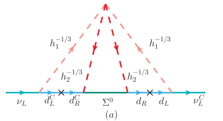
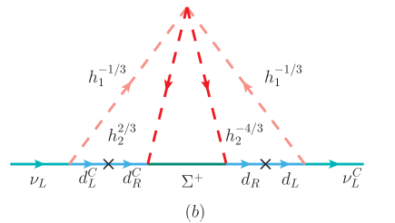
Figure 1: Three-loop diagrams contributing to neutrino masses, mediated via neutral (charged) fermion triplets. A third diagram (not displayed here) can be obtained by replacing $\Sigma^{+}$ by its charge conjugate state $\Sigma^{-}$, while also exchanging the internal $h_{2}^{2/3,-4/3}$ propagators of panel (b).

The computation of the different diagrams of Fig. 1 leads to the following contributions to neutrino masses (which are for simplicity cast in the weak interaction basis):

$$-i(m_{\nu})_{\alpha\beta}\,=\, 2\int\frac{d^{4}Q_{1}}{\left(2\pi\right)^{4}}\,\int\frac{d^{4}Q_{2}}{\left(2\pi\right)^{4}}\,\frac{i}{Q_{1}^{2}\,-\,m_{h_{1}}^{2}}\,\left(-2i\,y^{T}_{\alpha i}\right)\,P_{L}\,\frac{i}{\not{Q}_{1}\,-\,m_{D_{i}}}\,\times$$

$$\int\frac{d^{4}k}{\left(2\pi\right)^{4}}\,\left(-i\,\tilde{y}^{T}_{ij}\right)\,P_{L}\,\frac{i\left(\not{k}\,+\,m_{\Sigma_{j}}\right)}{k^{2}-m_{\Sigma_{j}}^{2}}\,P_{L}\,\left(-i\,\tilde{y}_{jk}\right)\,\frac{i}{\left(k+Q_{1}\right)^{2}\,-\,m_{h_{2}}^{2}}\times$$

$$\left[-i(s_{a}\times\kappa_{c})\,\frac{\lambda_{h}}{2}-2i(s_{b}\times\kappa_{c})\,\lambda_{h}\right]\,\times$$

$$\frac{i}{\left(k\,-\,Q_{2}\right)^{2}\,-\,m_{h_{2}}^{2}}\,\frac{i}{\not{Q}_{2}\,-\,m_{D_{k}}}\,P_{L}\,\left(-2i\,y_{k\beta}\right)\,\frac{i}{Q_{2}^{2}\,-\,m_{h_{1}}^{2}},$$ (12)

in which $Q_{1,2}$ denotes the momenta of the internal down-type quarks, $m_{D}=\text{diag}(m_{d},m_{s},m_{b})$ is the diagonal down-quark mass matrix, and $P_{L,R}=(1\mp\gamma_{5})/2$. For clarity, we have explicitly highlighted the contributions of the four-scalar leptoquark vertices of diagrams (a) and (b) (as well as the $\Sigma^{-}$ counterpart of (b)), writing them as products of symmetry and colour factors, respectively $s$ and $\kappa_{c}$. Diagram (a) is associated with $s_{a}=4$, while (b)-like diagrams lead to $s_{b}=2$; for the colour factor one has $\kappa_{c}=15$, due to the possible distinct contractions of the four-scalar leptoquark vertex (in agreement with [75]).

Using the appropriate loop integrals, and after a Wick rotation we obtain

$${}(m_{\nu})_{\alpha\beta}\,=\,-30\,\frac{\lambda_{h}}{\left(4\pi^{2}\right)^{3}\,m_{h_{2}}}\,y^{T}_{\alpha i}\,m_{D_{i}}\,\tilde{y}^{T}_{ij}\,G\left(\frac{m_{\Sigma_{j}}^{2}}{m_{h_{2}}^{2}},\frac{m_{h_{1}}^{2}}{m_{h_{2}}^{2}}\right)\,\tilde{y}_{jk}\,m_{D_{k}}\,y_{k\beta},$$ (15)

where $m_{D}$ is again the diagonal down type mass matrix (in the computation of the loop integrals, the down-quark masses are neglected when compared to the heavier $h_{1,2}$ and $\Sigma$ masses in the loop), and we recall that $y$ ($\tilde{y}$) denotes the Yukawa couplings of the $Z_{2}$-even leptoquark $h_{1}$ to matter ($Z_{2}$-odd leptoquark $h_{2}$ and triplet fermion $\Sigma_{R}$ to down quarks); finally $G(a,b)$ is defined as

$$G\left(a,b\right)\,=\,\frac{\sqrt{a}}{8\,b^{2}}\,\int_{0}^{\infty}dr\,\frac{r}{r+a}\,\left[\int_{0}^{1}dx\ln\left(\frac{x\,\left(1-x\right)\,r\,+\,\left(1-x\right)\,b\,+\,x}{x\,\left(1-x\right)\,r\,+\,x}\right)\right]^{2}\,,$$ (16)

and in the case in which (for simplicity and without loss of generality) $m_{\Sigma}$ is assumed to be diagonal, $G({m_{\Sigma_{j}}^{2}}/{m_{h_{2}}^{2}},{m_{h_{1}}^{2}}/{m_{h_{2}}^{2}})$ will also be diagonal.

The neutrino mass eigenstates can be obtained using the transformation

$$m_{\nu}^{\text{diag}}\,\equiv\,{\text{diag}}(m_{\nu_{1}},m_{\nu_{2}},m_{\nu_{3}})\,=\,U^{T}_{i\alpha}\,(m_{\nu})_{\alpha\beta}\,U_{\beta i}\,,$$ (17)

where $U$ is the Pontecorvo-Maki-Nakagawa-Sakata (PMNS) unitary mixing matrix, which we parametrise as follows

$$U\,=\,\left(\begin{array}[c]{ccc}c_{12}c_{13}&c_{13}s_{12}&s_{13}e^{-i\delta_{D}}\\ -c_{23}s_{12}-c_{12}s_{13}s_{23}e^{i\delta_{D}}&c_{12}c_{23}-s_{12}s_{13}s_{23}e^{i\delta_{D}}&c_{13}s_{23}\\ s_{12}s_{23}-c_{12}c_{23}s_{13}e^{i\delta_{D}}&-c_{12}s_{23}-c_{23}s_{12}s_{13}e^{i\delta_{D}}&c_{13}c_{23}\end{array}\right)\cdot{\text{diag}}(1,e^{i\alpha/2},e^{i\beta/2})\,.$$ (18)

In the above, $s_{ij}\equiv\sin(\theta_{ij})$ and $c_{ij}\equiv\cos(\theta_{ij})$; $\delta_{D}$ is the CP violating Dirac phase while $\alpha$ and $\beta$ are Majorana phases.

It is important to notice that as can be seen from Eqs. (15) and (17), neutrino masses (and leptonic mixings) do indeed depend on both of the Yukawa couplings involving the leptoquarks, $y$ and $\tilde{y}$. In particular, the former will be at the source of a number of flavour transitions, including rare meson decays, neutral meson-antimeson oscillations as well as charged lepton flavour violating processes. This implies that a strong connection between neutrino phenomena and flavour nonuniversal processes is established via the flavour structure of the Yukawa matrix $y$.

In the absence of a complete framework proving a full theory of flavour (which would suggest a structure for $y$ and $\tilde{y}$), one can nevertheless parametrise one of the Yukawa couplings - for example, $\tilde{y}$ - using a modified Casas-Ibarra parametrisation [83], which further allows to accommodate neutrino oscillation data.

In order to construct the modified Casas-Ibarra parametrisation, we first notice that from Eqs. (15) and (17) one can write the diagonal neutrino mass matrix as

$$m^{\text{diag}}_{\nu}\,=\,U^{T}\;y^{T}\;m_{D}\;\tilde{y}^{T}\;F(\lambda_{h},m_{\Sigma},m_{h_{1,2}})\;\tilde{y}\;m_{D}\;y\;U\,,$$ (19)

in which we have omitted flavour (generation) indices for simplicity, and where

$$F(\lambda_{h},m_{\Sigma},m_{h_{1,2}})\,=\,\frac{30\,\lambda_{h}}{(4\pi^{2})^{3}\,m_{h_{2}}}\,G_{j}\left(\frac{m_{\Sigma_{j}}^{2}}{m_{h_{2}}^{2}},\frac{m_{h_{1}}^{2}}{m_{h_{2}}^{2}}\right)\,.$$ (20)

As noted before, for a diagonal $m_{\Sigma}$, $G$ and thus $F$ are also diagonal matrices in generation space, which allows to write the identity

$$(\sqrt{m^{\text{diag}}_{\nu}}^{-1}U^{T}\;y^{T}\;m_{D}\;{\tilde{y}}^{T}\;\sqrt{F})\,(\sqrt{F}\;\tilde{y}\;m_{D}\;y\;U\;\sqrt{m^{\text{diag}}_{\nu}}^{-1})\,=\,\mathbb{1}\,=\,{\cal R}^{T}\,{\cal R},$$ (21)

with ${\cal R}$ an arbitrary complex orthogonal matrix (${\cal R}^{T}{\cal R}=\mathbb{1}$) which can be parametrised in terms of three complex angles, $\theta_{i}$ ($i=1-3$). Finally, from Eq. (21) one obtains the modified Casas-Ibarra parametrisation, which allows to write the Yukawa couplings of the $h_{2}$ leptoquark in terms of observable quantities (light neutrino masses, leptonic mixings, down quark masses, triplet and leptoquark masses), and of two unknown quantities - the $h_{1}$ leptoquark Yukawa couplings and a complex orthogonal matrix - as

$$\tilde{y}\,=\,F^{-1/2}\;\mathcal{R}\;\sqrt{m^{\text{diag}}_{\nu}}\;U^{\dagger}y^{-1}m_{d}^{-1}\,.$$ (22)

The above parametrisation (which is in agreement to a similar approach carried in [75]), allows to write the couplings $\tilde{y}$ in terms of $y$ up to a complex orthogonal matrix. As will be discussed in detail in Section 8.1, once the approximate flavour texture of $y$ is inferred from various experimental constraints, that of $\tilde{y}$ can be derived (up to the mixings due to $\mathcal{R}$).

4 A viable dark matter candidate

Reinforcing the SM gauge group via a discrete $Z_{2}$ symmetry ensures the stability of the lightest state which is odd under $Z_{2}$. If the lightest $Z_{2}$-odd particle (LZoP) is neutral, and the strength of its interactions is such that its relic abundance is in agreement with observational data, then it can be indeed a viable dark matter candidate.

In our analysis we assume that the spectrum of the new states is such that one has $m_{\Sigma_{R}^{1}}<m_{h_{2}}$. At the tree level, all the components of a generation $\Sigma_{R}^{i}$ have the same mass $m_{\Sigma^{i,\text{tree}}}=m_{\Sigma^{i,\pm}}=m_{\Sigma^{i,0}}$. The degeneracy between the components is broken by EW radiative corrections, which render the charged states heavier than the neutral one. Dropping for simplicity the generation indices (in this section our discussion is focused on the components of the lighest triplet, $\Sigma_{R}^{1}$), the splitting between the neutral and charged components is given by [84]

$$\Delta_{m_{\Sigma}}\,=\,m_{\Sigma^{\pm}}\,-\,m_{\Sigma^{0}}\,=\,\frac{\alpha_{2}\,m^{\text{tree}}_{\Sigma}}{4\pi}\,\left[f_{\text{EW}}\left(x_{W\Sigma}\right)\,-\,\cos^{2}\theta_{w}f_{\text{EW}}\left(x_{Z\Sigma}\right)\right]\,,$$ (23)

with $x_{ij}=\frac{m_{i}}{m_{j}}$ and

$$f_{\text{EW}}(x)\,=\,-x^{2}\,+\,x^{4}\,\ln x\,+\,x\,(x^{2}-4)^{1/2}\,\left(1+\frac{x^{2}}{2}\right)\,\ln\left(-1-\frac{x}{2}\,(x^{2}-4)^{1/2}+\frac{x^{2}}{2}\right)\frac{x}{2},$$ (24)

and in which $\alpha_{2}=\alpha_{e}/\sin^{2}\theta_{w}$, with $\alpha_{e}$ the fine structure constant and $\theta_{w}$ the weak mixing angle. In the limit $m_{\Sigma}\gg M_{W,Z}$ (justified by negative searches at LHC and EW precision measurements), the EW radiative corrections are found to be of order $m_{\Sigma^{\pm}}-m_{\Sigma^{0}}\sim 166$ MeV. While the latter mass difference is enough to ensure that the neutral component of the lightest triplet, $\Sigma^{0}$, is indeed the LZoP, it is sufficiently small to be neglected in the subsequent (numerical) analysis.

The relic abundance of the LZoP $\Sigma^{0}$ is determined by its interactions and by the annihilation and coannihilation channels open in view of the particle mass spectrum. In addition to the Yukawa interactions with $h_{2}$, the $\Sigma_{R}$ triplets are subject to SU(2)_L gauge interactions. Since, as previously highlighted, we assume that $m_{\Sigma_{R}^{1}}<m_{h_{2}}$, the relic density of $\Sigma^{0}$ is, to first order approximation, solely determined by its gauge interactions, which govern the distinct annihilation and coannihilation channels (involving also the charged components $\Sigma^{\pm}$). In particular, the annihilation and coannihilation processes involve the following channels: $\Sigma^{0}\Sigma^{0}\rightarrow W^{\pm}W^{\mp}$ through $t$-channel $\Sigma^{\pm}$ exchange; $\Sigma^{0}\Sigma^{\pm}\rightarrow W^{\pm}Z^{0}$ via $t$-channel $\Sigma^{\pm}$ exchange; $\Sigma^{0}\Sigma^{\pm}\rightarrow W^{\pm}Z^{0},W^{\pm}H,\bar{f}f^{\prime}$ (via $s$-channel $W^{\pm}$ exchange). Other processes involving the charged components of the triplet fermion must be also taken into account in the Boltzmann equations leading to the computation of the relic density. These include $\Sigma^{\pm}\Sigma^{\mp}\rightarrow Z^{0}Z^{0}(W^{\pm}W^{\mp})$ through $\Sigma^{\pm(0)}$ $t$-channel exchange, $\Sigma^{\pm}\Sigma^{\mp}\rightarrow W^{\pm}W^{\mp},Z^{0}H,\bar{f}f$ ($s$-channel via $Z^{0}$ mediation), and finally $\Sigma^{\pm}\Sigma^{\pm}\rightarrow W^{\pm}W^{\pm}$ through $\Sigma^{0}$ exchange ($t$-channel).

The relevant cross sections for the above mentioned processes are given by [85]

$$\sigma(\Sigma^{0}\Sigma^{0})|\bar{v}|\,\simeq\,2\pi\,\frac{\alpha_{2}^{2}}{m_{\Sigma}^{2}},\quad\sigma(\Sigma^{0}\Sigma^{\pm})|\bar{v}|\,\simeq\,2\pi\,\frac{29\,\alpha_{2}^{2}}{16\,m_{\Sigma}^{2}}\,,$$

$$\sigma(\Sigma^{+}\Sigma^{-})|\bar{v}|\,\simeq\,2\pi\,\frac{37\,\alpha_{2}^{2}}{16\,m_{\Sigma}^{2}}\,,\quad\sigma(\Sigma^{\pm}\Sigma^{\pm})|\bar{v}|\,\simeq\,2\pi\,\frac{\alpha_{2}^{2}}{2m_{\Sigma}^{2}}\,,$$ (25)

where only the coefficients $a_{ij}$ are kept in the relative velocity ($\bar{v}$) expansion of the cross section, i.e. $\sigma_{ij}|\bar{v}|=a_{ij}+b_{ij}\bar{v}^{2}$.

The computation of the relic abundance follows closely the method of [86], in which the freeze-out temperature of the LZoP $\Sigma^{0}$ ($x_{f}\equiv m_{\Sigma}/T_{f}$) is obtained in terms of the thermally averaged effective cross section $\langle\sigma_{\text{eff}}|\bar{v}|\rangle$. The relevant channels above referred to contribute to the thermally averaged effective cross section $\langle\sigma_{\text{eff}}|\bar{v}|\rangle$ as

$$\langle\sigma_{\text{eff}}|\bar{v}|\rangle\,=\, \frac{g_{0}^{2}}{g_{\text{eff}}^{2}}\,\sigma(\Sigma^{0}\Sigma^{0})|\bar{v}|\,+\,4\,\frac{g_{0}\,g_{\pm}}{g_{\text{eff}}^{2}}\,\sigma(\Sigma^{0}\Sigma^{\pm})|\bar{v}|\,\left(1+\frac{\Delta_{m_{\Sigma}}}{m_{\Sigma}}\right)^{3/2}\exp\left(-\frac{\Delta_{m_{\Sigma}}}{m_{\Sigma}}\,x_{f}\right)\,+$$ (26)

$$+\frac{g_{\pm}^{2}}{g_{\text{eff}}^{2}}\,\left[\,2\,\sigma(\Sigma^{+}\Sigma^{-})|\bar{v}|\,+\,2\,\sigma(\Sigma^{\pm}\Sigma^{\pm})|\bar{v}|\right]\left(1+\frac{\Delta_{m_{\Sigma}}}{m_{\Sigma}}\right)^{3}\exp\left(-2\frac{\Delta_{m_{\Sigma}}}{m_{\Sigma}}x_{f}\right)\,,$$

and the freeze-out temperature is then recursively given by

$$x_{f}\,\equiv\,\frac{m_{\Sigma}}{T_{f}}\,=\,\ln\left(\frac{0.038\;g_{\text{eff}}\;M_{\text{Pl}}\;m_{\Sigma}\;\langle\sigma_{\text{eff}}|\bar{v}|\rangle}{g_{\ast}^{1/2}x_{f}^{1/2}}\right)\,,$$ (27)

in which $g_{\ast}\sim 106.75$ is the total number of effective relativistic degrees of freedom the freeze-out, and $M_{\text{Pl}}=1.22\times 10^{19}$ GeV is the Planck scale. The quantity $g_{\text{eff}}$ is related to the degrees of freedom of the triplet components, $g_{0}=2$ and $g_{\pm}=2$, respectively for $\Sigma^{0}$ and $\Sigma^{\pm}$ and to $\Delta_{m_{\Sigma}}$ (the mass splitting between the charged and neutral components of $\Sigma_{R}$), and can be written as

$$g_{\text{eff}}\,=\,g_{0}\,+\,2\,g_{\pm}\left(1+\frac{\Delta_{m_{\Sigma}}}{m_{\Sigma}}\right)^{3/2}\exp\left(-\frac{\Delta_{m_{\Sigma}}}{m_{\Sigma}}\,x_{f}\right)\,.$$ (28)

Finally, the relic abundance is given by

$$\Omega\,h^{2}\,=\,\frac{1.07\times 10^{9}\,x_{f}}{g_{\ast}^{1/2}\;M_{\text{Pl}}({\text{GeV}})\;I_{a}},$$ (29)

with $I_{a}$ the annihilation integral, which is defined as

$$I_{a}\,=\,x_{f}\,\int_{x_{f}}^{\infty}x^{-2}\,a_{\text{eff}}\;dx\,.$$ (30)

In the above, one has used the approximation $a_{\text{eff}}\sim\sigma_{\text{eff}}|\bar{v}|$ (we recall that we have not taken into account the second and higher order terms in the relative velocity expansion of the effective cross section).

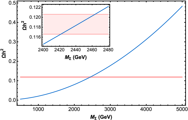
Figure 2: Estimated relic abundance (see text for details) of the dark matter candidate, $\Sigma^{0}$, as a function of its mass. The rose-coloured band corresponds to the latest observational data $\Omega h^{2}=0.1198\pm 0.0015$ [87].

For our purpose of constraining the parameter space of the model, we will rely on a simple iterative solution of Eq. (29), which allows to infer first limits on the values of $m_{\Sigma^{1}_{R}}$ leading to a relic density in agreement with the most recent observational data [87],

$$\Omega\,h^{2}\,=\,0.1186\,\pm\,0.0020\,.$$ (31)

The results of this (approximative) numerical analysis are displayed in Fig. 2, which reveals that having an LZoP mass in the range $2.425\;{\text{TeV}}<m_{\Sigma}<2.465\;{\text{TeV}}$ leads to a dark matter relic abundance in agreement with the latest data. In what follows, we will use $m_{\Sigma}\sim 2.45{\text{TeV}}$ as an illustrative benchmark value for the lightest fermion triplet mass.

Although already mentioned, we nevertheless stress again that several approximations were done in our computation of the relic abundance; moreover, one should also explicitly solve the coupled Boltzmann equations to numerically obtain the allowed mass range of the LZoP (the lightest $\Sigma^{0}$). Other than complying with the dark matter relic abundance, the potential candidate is also subject to the increasingly strong constraints from direct and indirect searches (see, e.g. [84, 88]); a detailed discussion of the latter (and the dedicated facilities) lies beyond the scope of this work.

5 Addressing the $\boldsymbol{B}$ meson decay anomalies

As can be seen from the interaction Lagrangian of Eq. (10), the scalar leptoquark $h_{1}$ couples to both down-type quarks and charged leptons, the couplings having a priori a non-trivial structure in flavour space. This will open the door to new contributions to numerous rare flavour changing transitions and decays, and - most importantly - can potentially lead to lepton flavour non-universal effects, such as those currently suggested by the reported LHCb anomalies.

In this section we will explore to which extent the current model succeeds in addressing the $B$ meson decay anomalies, $R_{K^{(\ast)}}$ and $R_{D^{(\ast)}}$, respectively associated with neutral and charged current transitions. The abundant constraints arising from negative searches for NP effects in meson oscillation and decays, as well as in charged lepton flavour violating observables will be discussed in Sections 6 and 7.

5.1 Neutral current anomalies: $R_{K}$ and $R_{K^{\ast}}$

As mentioned in the Introduction, recent measurements [3, 6] of the ratios of branching ratios of $B\to K(K^{\ast})\ell\ell$ decays into pairs of muons over those into di-electrons exhibit non-negligible deviations when compared to the SM predictions [4, 5]; as already stated one has

$$R_{K[1,6]}\,=\,0.745\,\pm_{0.074}^{0.090}\,\pm\,0.036,\,\quad R_{K}^{\text{SM}}\,=\,1.00,\pm\,0.01$$ (32)

$$R_{K^{*}[0.045,1.1]}\,=\,0.66^{+0.11}_{-0.07}\,\pm\,0.03\,,\quad R_{K^{*}[0.045,1.1]}^{\text{SM}}\,\sim\,0.92\pm 0.02$$

$$R_{K^{*}[1.1,6]}\,=\,0.69^{+0.11}_{-0.07}\,\pm 0.05\,,\quad R_{K^{*}[1.1,6]}^{\text{SM}}\,\sim\,1.00\pm 0.01\,,$$

where the dilepton invariant mass squared bin (in $\text{GeV}^{2}$) is identified by the subscript. The comparison of SM predictions with observation respectively reveals deviations of $2.6\sigma$, $2.4\sigma$ and $2.5\sigma$.

For the leptoquark mass regime considered here (multi-TeV), the neutral current effects induced by the heavy degrees of freedom (SM and NP contributions) in the quark level transitions $d_{j}\to d_{i}\ell^{+}\ell^{-}$ can be described by the following effective Hamiltonian [89, 90]

$$\mathcal{H}(d_{j}\to d_{i}\ell^{+}\ell^{-}) = -\frac{4\,G_{F}}{\sqrt{2}}V_{tj}\,V_{ti}^{\ast}\left[C_{7}^{ij}\,\mathcal{O}^{ij}_{7}+C_{7^{\prime}}^{ij}\,\mathcal{O}^{ij}_{7^{\prime}}\,+\sum_{{}_{X=9,10,S,P}}\left(C_{X}^{ij;\ell\ell^{\prime}}\,\mathcal{O}_{X}^{ij;\ell\ell^{\prime}}\,+\,C_{X^{\prime}}^{ij;\ell\ell^{\prime}}\,\mathcal{O}_{X^{\prime}}^{ij;\ell\ell^{\prime}}\right)\,+\right.$$ (33)

$$\left.\phantom{[C_{7}^{ij}\,\mathcal{O}^{ij}_{7}+C_{7^{\prime}}^{ij}\,\mathcal{O}^{ij}_{7^{\prime}}\,+}+\,C^{ij;\ell\ell^{\prime}}_{T}\,\mathcal{O}^{ij;\ell\ell^{\prime}}_{T}+\,C_{T5}^{ij;\ell\ell^{\prime}}\,\mathcal{O}^{ij;\ell\ell^{\prime}}_{T5}\right]+\,\text{H.c.}\;,$$

in which $G_{F}$ is the Fermi constant and $V$ is the CKM mixing matrix. The effective operators present in the above equation can be defined as (for simplicity, hereafter we drop the $ij$ superscripts, which are set to $i,j=s,b$ for the process $b\to s\ell^{+}\ell^{-}$):

$$\mathcal{O}_{7}\,=\,\frac{em_{d_{j}}}{(4\pi)^{2}}\,(\bar{d}_{i}\sigma_{\mu\nu}P_{R}d_{j})\,F^{\mu\nu}\,,$$

$$\mathcal{O}_{9}^{\ell\ell^{\prime}}\,=\,\frac{e^{2}}{(4\pi)^{2}}\,(\bar{d}_{i}\gamma^{\mu}P_{L}d_{j})(\bar{\ell}\gamma_{\mu}\ell^{\prime})\,,\quad\mathcal{O}_{10}^{\ell\ell^{\prime}}\,=\,\frac{e^{2}}{(4\pi)^{2}}\,(\bar{d}_{i}\gamma^{\mu}P_{L}d_{j})(\bar{\ell}\gamma_{\mu}\gamma_{5}\ell^{\prime})\,,$$

$$\mathcal{O}_{S}^{\ell\ell^{\prime}}\,=\,\frac{e^{2}}{(4\pi)^{2}}\,(\bar{d}_{i}P_{R}d_{j})(\bar{\ell}\ell^{\prime})\,,\quad\mathcal{O}_{P}^{\ell\ell^{\prime}}\,=\,\frac{e^{2}}{(4\pi)^{2}}\,(\bar{d}_{i}P_{R}d_{j})(\bar{\ell}\gamma_{5}\ell^{\prime})\,,$$

$$\mathcal{O}^{\ell\ell^{\prime}}_{T}\,=\,\frac{e^{2}}{(4\pi)^{2}}\,(\bar{d}_{i}\sigma_{\mu\nu}d_{j})(\bar{\ell}\sigma^{\mu\nu}\ell^{\prime})\,,\quad\mathcal{O}^{\ell\ell^{\prime}}_{T5}\,=\,\frac{e^{2}}{(4\pi)^{2}}\,(\bar{d}_{i}\sigma_{\mu\nu}d_{j})(\bar{\ell}\sigma^{\mu\nu}\gamma_{5}\ell^{\prime})\,.$$ (34)

In the above, $e$ is the electric charge and $\sigma_{\mu\nu}=i[\gamma_{\mu},\gamma_{\nu}]/2$. The set of primed operators ($X^{\prime}=7^{\prime},9^{\prime},10^{\prime},S^{\prime},P^{\prime}$) comprises those of opposite chirality, and can be obtained by replacing $P_{L}\leftrightarrow P_{R}$ in the quark currents. The contribution of the right-handed current operators is negligible in the SM. Flavour universality of lepton-gauge interactions in the SM implies that the Wilson coefficients of operators $\mathcal{O}_{i}^{\ell\ell}$ are universal for all lepton flavours $(\ell=e,\mu,\tau)$, and the strict conservation of individual lepton flavour further precludes cLFV Wilson coefficients $C_{i}^{\ell\ell^{\prime}}$ $(\ell\neq\ell^{\prime})$.

In the present scalar leptoquark model, once the heavy degrees of freedom have been integrated out (under the assumption that $M_{t,W,Z}^{2}\ll m_{h_{1}}^{2}$), the NP effective Hamiltonian is given by [91]

$$\mathcal{H}^{\text{NP}}(b\to s\ell^{-}\ell^{\prime+})\,=\,-\frac{y_{b\ell^{\prime}}\,y_{s\ell}^{\ast}}{m_{h_{1}}^{2}}\,(\bar{s}\,\gamma^{\mu}\,P_{L}\,b)\,(\bar{\ell}\,\gamma_{\mu}\,P_{L}\,\ell^{\prime})+\text{H.c.}\,;$$ (35)

comparing the above with the operator basis of Eq. (33), it is possible to infer the following contributions to the Wilson coefficients

$$C_{9}^{\ell\ell^{\prime}}\,=\,-C_{10}^{\ell\ell^{\prime}}\,=\,\frac{\pi\,v^{2}}{\alpha_{e}\,V_{tb}\,V_{ts}^{\ast}}\,\frac{y_{b\ell^{\prime}}\,y_{s\ell}^{\ast}}{m_{h_{1}}^{2}}\,.$$ (36)

The deviations from the SM lepton flavour universality imply that the modifications to the Wilson coefficients are necessarily non-universal for the muon and electron entries; the model-independent fit of [91] suggests the following corrections at the $1\sigma$ range:

$$\text{Re}[C_{9,\text{NP}}^{\mu\mu}\,-\,C_{10,\text{NP}}^{\mu\mu}-(\mu\leftrightarrow e)] \sim\,-1.1\pm 0.3\,,$$ (37)

$$\text{Re}[C_{9^{\prime}}^{\mu\mu}-C_{10^{\prime}}^{\mu\mu}\,-\,(\mu\leftrightarrow e)] \sim\,0.1\pm 0.4\,,$$ (38)

(notice that the second constraint is compatible with zero, and can be fulfilled by setting $C_{9^{\prime},10^{\prime}}^{\mu\mu,ee}=0$). In the present NP construction, leptoquark couplings to both muons and electrons are present, and are of left-handed nature. Given that $C_{9}^{\ell\ell^{\prime}}=-C_{10}^{\ell\ell^{\prime}}$ (cf. Eq. (36)), the best fit to the $C_{9,10\text{ NP}}^{\mu\mu,ee}$ Wilson coefficients of Eq. (36) can be recast as

$$-1.4\,\lesssim\,2\,\text{Re}[C_{9,{\rm NP}}^{\mu\mu}\,-\,C_{9,{\rm NP}}^{ee}]\,\lesssim\,-0.8\,.$$ (39)

Global fits to a large number of observables probing lepton flavour universality in relation to $b\to s\mu^{\pm}\mu^{\mp}$, $b\to se^{\pm}e^{\mp}$ and $b\to s\gamma$ processes also suggest NP scenarios consistent with the above fit to the LFUV $R_{K^{(*)}}$ observables. A common conclusion that can be generically drawn is that the NP responsible for the observed discrepancies in $b\to s$ data appears to predominantly couple to muons, and is strongly manifest in vector operators (as ${\cal O}_{9,10}^{\mu\mu}$). Recent studies and fits by a number of authors (see, e.g. [92, 93, 94, 95, 5]) advocate NP contribution to $C_{9}^{\mu\mu}$ ($\sim-1$) only, or then SU$(2)_{L}$ invariant scenarios ($C_{9}^{\mu\mu}=-C_{10}^{\mu\mu}\sim-0.6$) as preferred NP solutions to alleviate the tensions with the SM.

In terms of the $h_{1}$ leptoquark mass and couplings, the expression of Eq. (39) translates into the following condition [91]

$$0.64\times 10^{-3}\,\lesssim\,\frac{\text{Re}[y_{b\mu}\,y_{s\mu}^{\ast}\,-\,y_{be}\,y_{se}^{\ast}]}{(m_{h_{1}}/1\text{TeV})^{2}}\,\lesssim\,1.12\times 10^{-3}\,.$$ (40)

In Fig. 3, for an illustrative value of $m_{h_{1}}=1.5~{}\text{TeV}$, we display the $(y_{b\ell}\,y_{s\ell})$ parameter space consistent with the observed values of $R_{K}$ and $R_{K^{\ast}}$ at the $1\sigma$ level, in agreement with Eq. (40). The inset plot shows the regimes of $y_{b\mu}$ and $y_{s\mu}$ compatible with $R_{K^{(\ast)}}$ (also for $m_{h_{1}}=1.5~{}\text{TeV}$, and for fixed values of the couplings to the electron, $y_{be}y_{se}=2\times 10^{-5}$).

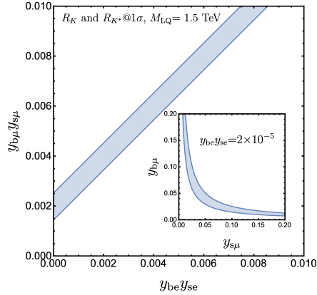
Figure 3: On the main plot, 1$\sigma$ region in the $(y_{be}\,y_{se}-y_{b\mu}\,y_{s\mu})$ parameter space consistent with $R_{K}$ and $R_{K^{\ast}}$ data, cf. Eq. (40), for an example with $m_{h_{1}}=1.5~{}\text{TeV}$. On the inset plot we display the $R_{K^{(\ast)}}$ allowed region in the $(y_{b\mu}-y_{s\mu})$ plane, for fixed values of the leptoquark electron Yukawa couplings $y_{be}y_{se}=2\times 10^{-5}$ (again for $m_{h_{1}}=1.5~{}\text{TeV}$).

5.2 Anomalies in $\boldsymbol{b\to c\ell^{-}\bar{\nu}_{i}}$: $\boldsymbol{R_{D^{(*)}}}$

Several experimental collaborations have also reported deviations from lepton flavour universality in association with $B\to D^{\ast}\ell\bar{\nu}$ decays (charged current $b\to c\ell\bar{\nu}_{i}$ transitions). A scalar charged leptoquark with non-trivial couplings to quarks and leptons can mediate $d_{k}\to u_{j}\ell\bar{\nu}_{i}$ transitions at the tree level, via the exchange of a charged $h_{1}^{1/3}$. The SM effective Hamiltonian governing these transitions is thus modified as follows:

$$\mathcal{H}_{\text{eff}}(d_{k}\to u_{j}\ell\bar{\nu}_{i})\, =\,\mathcal{H}_{\text{eff}}^{\text{SM}}\,+\,\mathcal{H}_{\text{eff}}^{\text{NP}}$$

$$=\,\left[\frac{4\,G_{F}}{\sqrt{2}}\,V_{jk}\,U_{\ell i}\,-\,\frac{(y\,U)_{ki}\,(V\,y^{\ast})_{j\ell}}{2\,m_{h_{1}}^{2}}\right]\,\left(\bar{u}_{j}\,\gamma^{\mu}\,P_{L}\,d_{k}\right)\,\left(\bar{\ell}\,\gamma_{\mu}\,P_{L}\,\nu_{i}\right)+\,\text{H.c.}$$

$$=\,\frac{4\,G_{F}}{\sqrt{2}}\,V_{jk}\,\left[U_{\ell i}\,-\,\frac{v^{2}}{4\,V_{cb}\,m_{h_{1}}^{2}}\,(yU)_{ki}\,(Vy^{\ast})_{j\ell}\right]\,\left(\bar{u}_{j}\,\gamma^{\mu}\,P_{L}\,d_{k}\right)\,\left(\bar{\ell}\,\gamma_{\mu}\,P_{L}\,\nu_{i}\right)+\text{H.c.}\;.$$ (41)

The experimentally measured decay probability is an incoherent sum over the (untagged) neutrino flavour $i$; one thus finds

$$\left|\mathcal{A}(d_{k}\to u_{j}\ell\bar{\nu})\right|^{2} =\,\sum_{i}\left|\mathcal{A}_{\text{SM}}\right|^{2}\,\left|U_{\ell i}\,-\,\frac{v^{2}}{4\,V_{jk}\,m_{h_{1}}^{2}}\,(yU)_{ki}\,(Vy^{\ast})_{j\ell}\right|^{2}$$

$$= \,\left|\mathcal{A}_{\text{SM}}\right|^{2}\,\left[1\,+\,|x_{j\ell}|^{2}\,\sum_{i}|y_{ki}|^{2}\,-\,2\,\text{Re}\left(x_{j\ell}\,y_{k\ell}\right)\right]\,,$$ (42)

where $x_{j\ell}=(Vy^{\ast})_{j\ell}\left(v^{2}/4V_{cb}m_{h_{1}}^{2}\right)$, and in which one has used the unitarity of the PMNS matrix. The SM width for the decay $B\to D^{\ast}\ell\bar{\nu}$ (i.e., for $d_{k}=b,\,u_{j}=c$) will thus be corrected by an overall factor

$$\Gamma(B\,\to\,D^{\ast}\,\ell\,\bar{\nu})\,=\,\Gamma_{\text{SM}}(B\,\to\,D^{\ast}\,\ell\,\bar{\nu})\,\left[1\,+\,|x_{c\ell}|^{2}\,\sum_{i=e,\mu,\tau}|y_{bi}|^{2}\,-\,2\,\text{Re}\left(x_{c\ell}\,y_{b\ell}\right)\right]\,.$$ (43)

Pure leptoquark contributions are suppressed by an additional $v^{2}/m_{h_{1}}^{2}$ factor with respect to the SM-NP interference term, and can be hence neglected as a first approximation.

Defining $R_{D^{(\ast)}}$ as the ratio of the decay widths of tau and muon modes - that is, $R_{D^{(\ast)}}=\text{BR}(B\to D^{(\ast)}\tau\bar{\nu})/\text{BR}(B\to D^{(\ast)}\mu\bar{\nu})$, one can further construct the double ratio

$$\frac{R_{D}}{R_{D,\,\text{SM}}}\,=\,\frac{R_{D^{\ast}}}{R_{D^{\ast},\,\text{SM}}}\,=\,\frac{1-2\,\text{Re}\left(x_{c\tau}\,y_{b\tau}\right)}{1-2\,\text{Re}\left(x_{c\mu}\,y_{b\mu}\right)}\,,$$ (44)

(equal to one in the absence of NP). After combining current experimental world averages with the SM predictions, the current anomalous data can be parametrised as

$$\frac{R_{D}}{R_{D,\,\text{SM}}}\,=\,1.36\pm 0.15\,,\quad\frac{R_{D^{\ast}}}{R_{D^{\ast},\,\text{SM}}}\,=\,1.21\pm 0.06\,,$$ (45)

in which the statistical and systematical errors have been added in quadrature. Similar ratios comparing distinct final state lepton flavours can be built to test possible LFUV in the corresponding sectors. For example, the Belle Collaboration has reported measurements of the ratios $R_{D^{(\ast)}}^{\mu/e}=\text{BR}(B\to D^{(\ast)}\mu\bar{\nu})/\text{BR}(B\to D^{(\ast)}e\bar{\nu})$, which probe lepton flavour universality between electron and muon modes. The experimental values $R_{D}^{\mu/e,\text{exp}}=0.995\pm 0.022\pm 0.039$ [96] and $R_{D^{\ast}}^{e/\mu,\text{exp}}=1.04\pm 0.05\pm 0.01$ [97] are consistent with the SM expectation, $\sim 1$. The averaged value of both measurements is $R_{D^{(\ast)}}^{\mu/e,\text{exp}}=0.977\pm 0.043$.

In the present leptoquark model, the ratio $R_{D^{(\ast)}}^{\mu/e}$ is given by the appropriately modified version of Eq. (44),

$$\frac{R_{D^{(\ast)}}^{\mu/e}}{R_{D^{(\ast)},\text{ SM}}^{\mu/e}}\,=\,\frac{1\,-\,2\,\text{Re}\left(x_{c\mu}\,y_{b\mu}\right)}{1\,-\,2\,\text{Re}\left(x_{ce}\,y_{be}\right)}\,.$$ (46)

After having detailed the leptoquark contributions to the meson observables currently exhibiting a significant deviation from the SM expectation, we now address other processes which - being in agreement with SM predictions (negative searches or compatible measurements) can constrain the masses of the new states and their couplings.

6 Constraints from rare meson decays and oscillations

Various observables involving mesons lead to important bounds on leptoquark couplings; here we discuss the (leptoquark) NP contributions to leptonic and semi-leptonic meson decays (occurring at the tree level), and to meson oscillations and rare radiative decays, both at the loop level. The SM predictions and current experimental bounds for the processes here discussed are summarised in Table 2. The stringent bounds on NP contributions arising from the now observed decay $B_{s}\to\mu^{+}\mu^{-}$ are not discussed here, as they have been implicitly taken into account in defining the allowed ranges for $C_{10,\text{NP}}^{\mu\mu}$ and the $y_{22,23}$ Yukawa couplings in the previous section. Likewise, we do not include the constraints arising from semileptonic $K$-decays into charged dileptons ($K\to\pi\ell\ell$), as theoretical (SM) predictions are plagued by important uncertainties, and are not yet up to par with the precision of the experimental results (see for example [105, 106]).

Observables	SM prediction	Experimental data
$\text{BR}(K^{+}\to\pi^{+}\nu\bar{\nu})$	$(8.4\pm 1.0)\times 10^{-11}\phantom{|}{}^{\phantom{|}}_{\phantom{|}}$[98]	$17.3^{+11.5}_{-10.5}\times 10^{-11}\phantom{|}{}^{\phantom{|}}_{\phantom{|}}$[99] $<11\times 10^{-10}\phantom{|}{}^{\phantom{|}}_{\phantom{|}}$[100]
$\text{BR}(K_{L}\to\pi^{0}\nu\bar{\nu})$	$(3.4\pm 0.6)\times 10^{-11}\phantom{|}{}^{\phantom{|}}_{\phantom{|}}$[98]	$\leq 2.6\times 10^{-8}\phantom{|}{}^{\phantom{|}}_{\phantom{|}}$[101]
$R_{K}^{\nu\nu}$, $R_{K^{\ast}}^{\nu\nu}$ $\phantom{a}{}^{\phantom{|}}_{\phantom{|}}$ ($B\to K^{(\ast)}\nu\bar{\nu}$)	$R_{K^{(\ast)}}^{\nu\nu}=1$	$R_{K}^{\nu\nu}<3.9$ $\phantom{a}{}^{\phantom{|}}_{\phantom{|}}$[102] $R_{K^{\ast}}^{\nu\nu}<2.7\phantom{|}^{\phantom{|}}_{\phantom{|}}$[102]
$B_{s}^{0}-\bar{B}_{s}^{0}$ $\phantom{a}{}^{\phantom{|}}_{\phantom{|}}$ (mixing parameters)	$\Delta_{s}=|\Delta_{s}|e^{i\phi_{s}}=1$ $\phantom{a}{}^{\phantom{|}}_{\phantom{|}}$ $\phi_{s}=0$	$|\Delta_{s}|=1.01^{+0.17}_{-0.10}\phantom{|}{}^{\phantom{|}}_{\phantom{|}}$[103], $\phi_{s}[^{\circ}]=1.3^{+2.3}_{-2.3}\phantom{|}{}^{\phantom{|}}_{\phantom{|}}$[103]
$K^{0}-\bar{K}^{0}$ $\phantom{a}{}^{\phantom{|}}_{\phantom{|}}$ $\Delta m_{K}/(10^{-15}\text{GeV})$	$3.1(1.2)\phantom{|}^{\phantom{|}}_{\phantom{|}}$[104]	$3.484(6)\phantom{|}^{\phantom{|}}_{\phantom{|}}$[1]
$\text{BR}(K_{L}\to\mu e)$	—	$<4.7\times 10^{-12}\phantom{|}{}^{\phantom{|}}_{\phantom{|}}$[1]
$\text{BR}(B_{s}\to\mu e)$	—	$<1.1\times 10^{-8}\phantom{|}{}^{\phantom{|}}_{\phantom{|}}$[1]

Table 2: Relevant observables and current experimental bounds for leptonic and semi-leptonic meson decays and neutral meson anti-meson oscillations discussed in this section.

6.1 Rare $\boldsymbol{K}$ and $\boldsymbol{B}$ meson decays: $\boldsymbol{K\to\pi\nu_{\ell}\bar{\nu}_{\ell^{\prime}}}$ and $\boldsymbol{B\to K^{(\ast)}\nu_{\ell}\bar{\nu}_{\ell^{\prime}}}$

The $s\to d\nu\nu$ and $b\to s\nu\nu$ transitions provide some of the most important constraints on NP scenarios aiming at addressing the anomalies in $R_{K^{(\ast)}}$ and $R_{D^{(\ast)}}$ data.

Following the convention of [107], at the quark level the $|\Delta S|=1$ rare decays $K^{+}\,(K_{L})\to\pi^{+}\,(\pi^{0})\,\nu_{\ell}\bar{\nu}_{\ell^{\prime}}$ and $B\to K^{(\ast)}\nu_{\ell}\bar{\nu}_{\ell^{\prime}}$ can be described by the following short-distance effective Hamiltonian for $d_{j}\to d_{i}\nu_{\ell}\bar{\nu}_{\ell^{\prime}}$ transitions [108, 109]

$$\mathcal{H}_{\text{eff}}({d_{j}\to d_{i}}\nu_{\ell}\bar{\nu}_{\ell^{\prime}}) = -\frac{4\,G_{F}}{\sqrt{2}}\,V_{ti}^{\ast}\,V_{tj}\,\frac{\alpha_{e}}{2\,\pi}\,\left[C_{L,ij}^{\ell\ell^{\prime}}\,\left(\bar{d}_{i}\,\gamma_{\mu}\,P_{L}\,d_{j}\right)\,\left(\bar{\nu}_{\ell}\,\gamma^{\mu}\,\,P_{L}\,\nu_{\ell^{\prime}}\right)\right.\,+$$ (47)

$$\phantom{-\frac{4\,G_{F}}{\sqrt{2}}\,V_{ti}^{\ast}\,V_{tj}\,\frac{\alpha_{e}}{2\,\pi}\,[}+\left.C_{R,ij}^{\ell\ell^{\prime}}\,\left(\bar{d}_{i}\,\gamma_{\mu}\,P_{R}\,d_{j}\right)\,\left(\bar{\nu}_{\ell}\,\gamma^{\mu}\,P_{L}\nu_{\ell^{\prime}}\right)\right]\,+\,\text{H.c.}\,,$$

in which $i,j$ denote the down-type flavour content of the final and initial state meson, respectively. In the SM, only the lepton flavour conserving left-handed operator is present; the associated Wilson coefficient $C_{L,ij}^{\ell\ell}$ corresponding to a $d_{j}\to d_{i}$ transition is given by

$$C_{L,ij}^{\ell\ell,\text{SM}}\,=\,-\frac{1}{\sin^{2}\theta_{w}}\,\left(X_{t}^{\text{SM}}\,+\,\frac{V_{ci}^{\ast}\,V_{cj}}{V_{ti}^{\ast}\,V_{tj}}\,X_{c}^{\ell}\right)\,.$$ (48)

In the above, $X_{t}^{\text{SM}}$ and $X_{c}^{\ell}$ ($\ell=e,\mu,\tau$) are the loop functions associated with the (lepton flavour conserving) contributions from the top and charm quarks, respectively. In the SM, computations of the top loop function (including Next-to-Leading Order QCD corrections [110, 111, 112] and the full two-loop electroweak corrections [113]) have led to the result $X_{t}^{\text{SM}}=1.481(9)$ [98]; the charm loop functions $X_{c}^{\ell}$ have been computed at NLO [112, 114] and at Next-to-NLO [115, 116], and their numerical value is given by $\frac{1}{3}\sum_{\ell}X_{c}^{\ell}/|V_{us}|^{4}=0.365\pm 0.012$.

Once the heavy leptoquark degrees of freedom have been integrated out, the general effective Hamiltonian describing the NP contribution to $d_{j}\to d_{i}\nu_{\ell}\bar{\nu}_{\ell^{\prime}}$ processes induced by $h_{1}$ is given by

$$\mathcal{H}_{\text{eff}}^{\text{LQ}}(d_{j}\to d_{i}\nu_{\ell}\bar{\nu}_{\ell^{\prime}})\,=\,-\frac{(y\,U)_{j\ell^{\prime}}\,(y\,U)_{i\ell}^{\ast}}{2m_{h_{1}}^{2}}\,\left(\bar{d}_{i}\,\gamma_{\mu}\,P_{L}\,d_{j}\right)\,\left(\bar{\nu}_{\ell}\,\gamma^{\mu}\,P_{L}\,\nu_{\ell^{\prime}}\right)\,,$$ (49)

and comparison with Eq. (47) leads to the following NP Wilson coefficient,

$$C_{L,ij}^{\ell\ell^{\prime},\,\text{LQ}}\,=\,\frac{\pi\,v^{2}}{\alpha_{e}\,V_{ti}^{\ast}V_{tj}}\,\frac{(yU)_{i\ell}^{\ast}\,(yU)_{j\ell^{\prime}}}{2\,m_{h_{1}}^{2}}\,,$$ (50)

in which we notice the presence of the PMNS matrix $U$, and the possibility that the tree level NP contribution, via the exchange of $h_{1}^{1/3}$, may lead to different lepton flavours in the final state, i.e. $\ell\neq\ell^{\prime}$.

$\boldsymbol{K\to\pi\nu_{\ell}\bar{\nu}_{\ell^{\prime}}}$ decays

The branching fraction for $K^{+}\to\pi^{+}\nu_{\ell}\bar{\nu}_{\ell^{\prime}}$ (corresponding to setting $i=d,j=s$ in the previous discussion) is given by [108, 109]

$$\text{BR}(K^{+}\,\to\,\pi^{+}\,\nu_{\ell}\,\bar{\nu}_{\ell^{\prime}})\,=\,\frac{\kappa_{+}\,(1+\Delta_{\rm em})}{3}\sum_{\ell,\ell^{\prime}=e,\mu,\tau}\left|\frac{V_{ts}^{\ast}\,V_{td}}{|V_{us}|^{5}}\,X_{t}^{\ell\ell^{\prime}}\,+\,\frac{V_{cs}^{\ast}\,V_{cd}}{|V_{us}|}\,\delta_{\ell\ell^{\prime}}\,\left(\frac{X_{c}^{\ell}}{|V_{us}|^{4}}\,+\,\Delta_{P_{c,u}^{\ell}}\right)\right|^{2}\,,$$ (51)

in which $\kappa_{+}=5.173(25)\times 10^{-11}\,(|V_{us}|/0.225)^{8}$, $\Delta_{\text{em}}=-0.003$ is the electromagnetic correction from photon exchanges and $\Delta_{P_{c,u}}=0.04(2)$ denotes the long-distance contribution from light quark loops, computed in [117]. The loop function associated with NP exchanges, $X_{t}^{\ell\ell^{\prime}}$, is given by

$${}X_{t}^{\ell\ell^{\prime}}\,=\,X_{t}^{\text{SM}}\,\delta_{\ell\ell^{\prime}}\,-\,\sin^{2}\theta_{w}\,C_{L,sd}^{\ell\ell^{\prime},\,\text{LQ}}\,.$$ (52)

Notice from both Eqs. (51, 52) that the SM top and charm contributions are lepton flavour conserving. Experimentally, the measurement of the charged kaon decay mode [99],

$$\text{BR}(K^{+}\,\to\,\pi^{+}\,\nu\,\bar{\nu})_{\text{exp}}\,=\,17.3^{+11.5}_{-10.5}\times 10^{-11}\,,$$ (53)

is expected to be improved in the near future by the results of the NA62 collaboration. The NA62 recent measurement [100] (one event) $\text{BR}(K^{+}\to\pi^{+}\nu\bar{\nu})_{\text{exp}}=28^{+44}_{-23}\times 10^{-11}$ still suffers from large statistical uncertainties, but these are expected to improve by an order of magnitude in coming months. The experimental bounds will allow to better constrain $X_{t}^{\ell\ell^{\prime}}$, and hence the leptoquark contributions, encoded in $C_{L,ij}^{\ell\ell^{\prime},\,\text{LQ}}$.

$\boldsymbol{K_{L}\to\pi^{0}\nu_{\ell}\nu_{\ell^{\prime}}}$ decays

The branching fraction for the neutral mode $K_{L}\to\pi^{0}\nu_{\ell}\nu_{\ell^{\prime}}$ can be written as [108, 109]

$$\text{BR}(K_{L}\,\to\,\pi^{0}\,\nu_{\ell}\,\bar{\nu}_{\ell^{\prime}})\,=\,\frac{\kappa_{L}}{3}\sum_{\ell,\ell^{\prime}=e,\mu,\tau}\left[\text{Im}\left(\frac{V_{ts}^{\ast}V_{td}}{|V_{us}|^{5}}\,X_{t}^{\ell\ell^{\prime}}\right)\right]^{2}\,,$$ (54)

with $\kappa_{L}=2.231(13)\times 10^{-10}\,(|V_{us}|/0.225)^{8}$ in the framework of the SM. Concerning the experimental status, only a $90\%$ C.L. bound has been reported for the decay [101]

$$\text{BR}(K_{L}\,\to\,\pi^{0}\,\nu\,\bar{\nu})_{\text{exp}}\,\leq\,2.6\times 10^{-8}\,,$$ (55)

which - as occuring for the charged decay modes - can also be used to constrain $X_{t}^{\ell\ell^{\prime}}$ and $C_{L,ij}^{\ell\ell^{\prime},\,\text{LQ}}$ (albeit leading to weaker constraints than those inferred from the $K^{+}\,\to\,\pi^{+}\,\nu\,\bar{\nu}$ mode).

$\boldsymbol{B\to K^{(\ast)}\nu_{\ell}\bar{\nu}_{\ell^{\prime}}}$

The branching ratio for the rare $B$ decay can be obtained by considering the general expressions for the effective Hamiltonian and NP Wilson coefficients, respectively given in Eqs. (47, 50), with $i=s,j=b$. It proves convenient to consider the following ratios $R^{\nu\nu}_{K^{(\ast)}}=\Gamma_{\text{SM + NP}}(B\to K^{(\ast)}\nu\nu)/\Gamma_{\text{SM}}(B\to K^{(\ast)}\nu\nu)$, which are then given by

$$R^{\nu\nu}_{K}\,=\,R^{\nu\nu}_{K^{\ast}}\,=\,\frac{1}{3\,|C_{L,bs}|^{2}}\sum_{\ell,\ell^{\prime}}\left|C_{L,bs}^{\ell\ell,\text{SM}}\,\delta_{\ell\ell^{\prime}}\,+\,C_{L,bs}^{\ell\ell^{\prime},\text{LQ}}\right|^{2}\,,$$ (56)

in which $C_{L,\text{SM}}^{\ell\ell}=-6.38(6)$ (for each neutrino flavour) [113]. The above expression can be explicitly cast in terms of the leptoquark masses and couplings as follows:

$$R^{\nu\nu}_{K^{(\ast)}} = \frac{1}{3\,\left|C_{L,bs}^{\ell\ell,\text{SM}}\right|^{2}}\,\left[3\,\left|C_{L,bs}^{\ell\ell,\text{SM}}\right|^{2}+\sum_{\ell\neq\ell^{\prime}}\left\lvert\left(\frac{\pi\,v^{2}}{\alpha_{e}\,V_{tb}\,V_{ts}^{\ast}}\right)\,\frac{y_{b\ell^{\prime}}\,y_{s\ell}^{\ast}}{2\,m_{h_{1}}^{2}}\right\rvert^{2}\right.\,+$$ (57)

$$\left.+\sum_{\ell=\ell^{\prime}}\left\{\left\lvert\left(\frac{\pi\,v^{2}}{\alpha_{e}\,V_{tb}\,V_{ts}^{\ast}}\right)\,\frac{y_{b\ell^{\prime}}\,y_{s\ell}^{\ast}}{2\,m_{h_{1}}^{2}}\right\rvert^{2}+2\,\text{Re}\left[{C_{L,bs}^{\ell\ell,\text{SM}}}^{\ast}\left(\frac{\pi\,v^{2}}{\alpha_{e}\,V_{tb}\,V_{ts}^{\ast}}\right)\,\frac{y_{b\ell}\,y_{s\ell}^{\ast}}{2\,m_{h_{1}}^{2}}\right]\right\}\right]\,.$$

The SM predictions for each of the modes are BR$(B^{+}\to K^{+}\nu\bar{\nu})=(4.0\pm 0.5)\times 10^{-6}$ [107] and BR$(B^{0}\to K^{\ast 0}\nu\bar{\nu})=(9.2\pm 1.0)\times 10^{-6}$ [107].

The latest experimental data from Belle [102] allows to infer the following bound, $R^{\nu\nu}_{K^{(\ast)}}<3.9(2.7)$ at $90\%$ C.L., which can be used to constrain combinations of leptoquark couplings (lepton flavour conserving and violating) as given in Eq. (57).

6.2 Neutral meson mixings and oscillations

Contributions to neutral meson mixings, $P-\bar{P}$ with $P=B^{0}_{s},B^{0}_{d},K^{0}$, arise both from SM box diagrams involving top and $W$’s, and from NP box diagrams involving charged (neutral) leptons and $h_{1}^{4/3}(h_{1}^{1/3})$ leptoquarks. These contributions can be described in terms of the following effective Hamiltonian for $|\Delta F|=2$ transitions

$$\mathcal{H}_{P}\,=\,(C_{P}^{\text{SM}}+C_{P}^{\text{NP}})\left(\bar{d}_{i}\,\gamma^{\mu}\,P_{L}\,d_{j}\right)\left(\bar{d}_{i}\,\gamma_{\mu}\,P_{L}\,d_{j}\right)\,+\text{H.c.},$$ (58)

where [57]

$$C_{P}^{\text{NP}}=\frac{3}{128\,\pi^{2}\,m_{h_{1}}^{2}}\left({\sum_{\ell}}y_{i\ell}^{\ast}\,y_{j\ell}\right)^{2}\,,$$ (59)

with $\{i,j\}$ respectively denoting $\{b,s\}$, $\{b,d\}$ or $\{d,s\}$ for $P=B^{0}_{s}$, $B^{0}_{d}$ or $K^{0}$ mesons.

Let us begin by discussing $B^{0}_{s}$ mixing, which is potentially the process most sensitive to the couplings $y_{b\ell}$ and $y_{s\ell}$ which are at the origin of the $R_{K^{(*)}}$ anomalies. Following [118, 103, 119], one can define the ratio of the total contribution (NP and SM) to the SM one

$$\Delta_{s}\,=\,|\Delta_{s}|\,e^{i\phi_{s}}\,=\,\frac{\langle B_{s}|\mathcal{H}_{B_{s}}|\bar{B}_{s}\rangle}{\langle B_{s}|\mathcal{H}^{\text{SM}}_{B_{s}}|\bar{B}_{s}\rangle}\,=\,1\,+\,\frac{C_{B_{s}}^{\text{NP}}}{C_{B_{s}}^{\text{SM}}}\,\equiv\,1\,+\,p_{s}\,.$$ (60)

In the leptoquark model we consider, the relative NP contribution $p_{s}$ can be cast as

$$p_{s}\,=\,\frac{3\,\left({\sum_{\ell}}\,y_{b\ell}\,y_{s\ell}^{\ast}\right)^{2}}{32\,m_{h_{1}}^{2}\,G_{F}^{2}\,M_{W}^{2}\,S_{0}(x_{t})\,(V_{tb}V^{\ast}_{ts})^{2}}\,,$$ (61)

where $S_{0}(x_{t})=2.35$ is the Inami-Lim function for the SM top quark box, with $x_{t}=M_{t}^{2}/M_{W}^{2}$ [120, 121]. Current global fits are compatible with the SM value ($\Delta^{\text{SM}}_{s}=1$): CKMfitter reports $|\Delta_{s}|=1.01^{+0.17}_{-0.10}$, $\phi_{s}[^{\circ}]=1.3^{+2.3}_{-2.3}$ [103], while for UTfit one has $|\Delta_{s}|=1.070\,{\pm 0.088}$, $\phi_{s}[^{\circ}]=0.054\,{\pm 0.951}$ [119]. Both analyses obtain their tightest $1\sigma$ constraints for imaginary NP contributions (i.e., $\arg p_{s}=-\pi/2$): $|p_{s}|<0.016$. In our study, and for simplicity, we will assume real Yukawa couplings $y_{q\ell}$ and a real $p_{s}$. In this case one has $p_{s}\geq 0$, and both analyses lead to $p_{s}<p_{s}^{\text{max}}\approx 0.17$, which translates into the following $1\sigma$ upper bound for the (real) $h_{1}$ leptoquark couplings:

$$\left|\sum_{\ell}y_{b\ell}\,y_{s\ell}\right|\,\lesssim 0.079\,\frac{m_{h_{1}}}{\text{TeV}}\,\sqrt{\frac{p_{s}^{\text{max}}}{0.17}}\,.$$ (62)

Following the same global analyses, a similar bound can be inferred from data on $B^{0}_{d}$ mixing (still in the case of real couplings), which leads to $p_{d}<p_{d}^{\textrm{max}}\approx 0.13$. One thus has

$$\left|\sum_{\ell}y_{b\ell}\,y_{d\ell}\right|\,\lesssim 0.069\,\frac{m_{h_{1}}}{\text{TeV}}\,\sqrt{\frac{p_{d}^{\text{max}}}{0.13}}\,.$$ (63)

For the case of $K^{0}-\bar{K}^{0}$ mixing, the SM effective coupling can be expressed as

$$C_{K}^{\text{SM}}\,=\,\frac{G_{F}^{2}\,M_{W}^{2}}{4\pi^{2}}\,F^{*}(x_{c},x_{t})\,$$ (64)

where $F(x_{c},x_{t})$ denotes the contribution of the distinct Inami-Lim functions, and is defined as

$$F(x_{c},x_{t})\,=\,(V_{cs}^{*}V_{cd})^{2}\,\eta_{cc}\,S_{0}(x_{c})\,+\,(V_{ts}^{*}V_{td})^{2}\,\eta_{tt}\,S_{0}(x_{t})\,+\,2\,V_{ts}^{*}V_{td}\,V_{cs}^{*}V_{cd}\,\eta_{ct}\,S_{0}(x_{c},x_{t})\,,$$ (65)

with $S_{0}(x_{c})\approx x_{c}+O(x_{c}^{2})=m_{c}^{2}/M_{W}^{2}$ [120, 121]; the coefficients $\eta_{cc}=1.87(76)$, $\eta_{tt}=0.5765(65)$ and $\eta_{ct}=0.496(47)$ encode NNLO QCD corrections [122, 104, 123, 124]. The last two terms in Eq. (65) can be safely neglected (as they are CKM-suppressed); the first (and dominant) term is associated to important theoretical uncertainties, $\mathcal{O}(40\%)$. From Eq. (59), the leptoquark contribution can be written as

$$p_{K}\,=\,\frac{C_{K}^{\text{NP}}}{C_{K}^{\text{SM}}}\,=\,\frac{3\,\eta_{tt}\,\tilde{r}\,\left({\sum_{\ell}}\,y_{s\ell}\,y_{d\ell}^{\ast}\right)^{2}}{32\,m_{h_{1}}^{2}\,G_{F}^{2}\,M_{W}^{2}\,S_{0}(x_{c})\eta_{cc}\,(V_{cs}V^{\ast}_{cd})^{2}}\,,$$ (66)

in which $\tilde{r}\approx 0.95$ allows to take into account the difference between the relevant scales ($M_{t}$ and $m_{h_{1}}$) [125].

Real couplings $y_{q\ell}$ only affect $\Delta m_{K}=\text{Re}\langle\bar{K}^{0}|\mathcal{H}_{K}|K^{0}\rangle/m_{K}$. Taking into account only the (dominant) first term of Eq. (65), the SM short distance contribution (cf. Eq. (64)) gives [104, 126]

$$(\Delta m_{K})_{\text{SM}}=(3.1\pm 1.2)\times 10^{-15}\text{GeV}=(0.89\pm 0.34)\,(\Delta m_{K})_{\text{exp}}$$ (67)

Comparing $(\Delta m_{K})_{\text{exp}}$ with the theoretical prediction ($(\Delta m_{K})_{\text{SM}}+(\Delta m_{K})_{\text{NP}}+(\Delta m_{K})_{\text{LD}}$), thus allows to obtain a conservative upper bound, $p_{K}<p_{K}^{\text{max}}\approx 0.45/0.55=0.81$. Leading to the latter limit, one has taken the lowest values of both $(\Delta m_{K})_{\text{SM}}$ ($\sim 55\%$) and the long distance (LD) contributions $(\Delta m_{K})_{\text{LD}}$, which are hard to evaluate but are expected to be positive like $p_{k}$ [126]. This translates into an upper bound on the leptoquark couplings:

$$\left|\sum_{\ell}y_{s\ell}\,y_{d\ell}\right|\,\lesssim 0.014\,\frac{m_{h_{1}}}{\text{TeV}}\,\sqrt{\frac{p_{K}^{\text{max}}}{0.81}}\,.$$ (68)

6.3 Leptonic decays of pseudoscalar mesons $\boldsymbol{P\to\ell^{-}\ell^{\prime+}}$

The leptonic decays of pseudoscalar mesons are known to provide stringent constraints on models of NP with modified lepton (and/or quark) sectors; leptoquark models are no exception, and in what follows we discuss some relevant modes of $K$ and $B$ mesons.

Leptonic $B_{s}$ meson decays $B_{(s)}^{0}\to\ell^{\pm}\ell^{\mp}$ are well predicted in the SM (the only hadronic uncertainty coming from the decay constant $f_{B_{s}}$). At present, only the $B_{s}\to\mu^{+}\mu^{-}$ decay mode has been observed, and it is in agreement with the SM. The LHC collaborations have reported values for its branching fraction of $(2.8^{+0.7}_{-0.6})\times 10^{-6}$ [127, 128]. As mentioned before, these bounds have been taken into account upon saturation of the $B$ decay anomalies.

For both $K$ and $B$ mesons, the cLFV leptonic decays have been shown to lead to important constraints on NP models: the cLFV $B$ decay modes are particularly relevant for leptoquark SM extensions [129]; although the hard to quantify long-distance QCD corrections render non-trivial an estimation of the leptonic $K_{L}$ decays [130]), the upper bounds on the cLFV mode $K_{L}\to\mu^{\pm}e^{\mp}$ prove to be one of the most stringent constraints on the couplings of leptoquarks to the first two generations of leptons and down-type quarks.

Following the effective Hamiltonian conventions adopted in Eq. (33), the decay width of $P\to\ell^{\pm}\ell^{\mp\prime}$ is governed by the $\mathcal{O}^{ij;\ell\ell^{\prime}}_{9}$ and $\mathcal{O}^{ij;\ell\ell^{\prime}}_{10}$ operators. In terms of the corresponding Wilson coefficients $C^{ij;\ell\ell^{\prime}}_{9,10}$, the decay width can be written [129]

$$\Gamma_{P\to\ell^{-}\ell^{\prime+}} =\,f_{P}^{2}\,m_{P}^{3}\,\frac{G_{F}^{2}\,\alpha_{e}^{2}}{64\,\pi^{3}}\left|V_{qj}\,V_{qi}^{*}\right|^{2}\,\beta(m_{P},m_{\ell},m_{\ell^{\prime}})\,\times$$

$$\times\Bigg{[}\left(1-\frac{(m_{\ell}+m_{\ell^{\prime}})^{2}}{m_{P}^{2}}\right)\left|\frac{m_{P}}{(m_{i}+m_{j})}(C^{ij;\ell\ell^{\prime}}_{S}-C^{ij;\ell\ell^{\prime}}_{S^{\prime}})+\frac{(m_{\ell}-m_{\ell^{\prime}})}{m_{P}}\left(C^{ij;\ell\ell^{\prime}}_{9}-C^{ij;\ell\ell^{\prime}}_{9^{\prime}}\right)\right|^{2}\,+$$

$$+\left(1-\frac{(m_{\ell}-m_{\ell^{\prime}})^{2}}{m_{P}^{2}}\right)\left|\frac{m_{P}}{(m_{i}+m_{j})}(C^{ij;\ell\ell^{\prime}}_{P}-C^{ij;\ell\ell^{\prime}}_{P^{\prime}})+\frac{(m_{\ell}+m_{\ell^{\prime}})}{m_{P}}\left(C^{ij;\ell\ell^{\prime}}_{10}-C^{ij;\ell\ell^{\prime}}_{10^{\prime}}\right)\right|^{2}\Bigg{]}\,,$$ (69)

in which $m_{i,j}$ denotes the mass of the meson valence quarks, the index $q$ refers to up-type quarks (the sum being dominated by the top quark contribution), and one defines

$$\beta(m_{P},m_{\ell},m_{\ell^{\prime}})\,=\,\sqrt{[1-(m_{\ell}-m_{\ell^{\prime}})^{2}/m_{P}^{2}]\,[1-(m_{\ell}+m_{\ell^{\prime}})^{2}/m_{P}^{2})]}\,.$$ (70)

7 Charged lepton flavour violating processes

Due to the presence of new states with non-negligible couplings to neutral and charged leptons, which are a source of LFUV, one expects that the model under consideration will give rise to important contributions to cLFV observables.

While most cLFV decays correspond to higher order (loop) processes, it is important to notice that transitions occurring in the presence of matter, such as neutrinoless muon-electron conversion in nuclei can now occur at the tree level. In the following, we address the contributions of the model to several cLFV observables, whose experimental status (current bounds and future sensitivities) is summarised in Table 3. The bounds on leptonic observables will give rise to stringent constraints on the parameter space of the model: other than neutrino oscillation data, bounds on several lepton flavour violating observables will play a significant rôle in identifying the regimes which can successfully lead to an explanation of the $B$ meson anomalies.

cLFV process	Current experimental bound	Future sensitivity
$\text{BR}(\mu\to e\gamma)$	$4.2\times 10^{-13}$ (MEG [131])	$6\times 10^{-14}$ (MEG II [132])
$\text{BR}(\tau\to e\gamma)$	$3.3\times 10^{-8}$ (BaBar [134])	$10^{-9}$ (Super B [135])
$\text{BR}(\tau\to\mu\gamma)$	$4.4\times 10^{-8}$ (BaBar [134])	$10^{-9}$ (Super B [135])
$\text{BR}(\mu\to 3e)$	$1.0\times 10^{-12}$ (SINDRUM [136])	$10^{-15(16)}$ (Mu3e [137])
$\text{BR}(\tau\to 3e)$	$2.7\times 10^{-8}$ (Belle [138])	$10^{-9}$ (Super B [135])
$\text{BR}(\tau\to 3\mu)$	$3.3\times 10^{-8}$ (Belle [138])	$10^{-9}$ (Super B [135])
$\text{CR}(\mu-e,\text{N})$	$7\times 10^{-13}$ (Au, SINDRUM [139])	$10^{-14}$ (SiC, DeeMe [140])
		$10^{-15(-17)}$ (Al, COMET [141])
		$3\times 10^{-17}$ (Al, Mu2e [142])
		$10^{-18}$ (Ti, PRISM/PRIME [143])

Table 3: Current experimental bounds and future sensitivities of cLFV processes included in the analysis.

7.1 Radiative decays $\ell\to\ell^{\prime}\gamma$

In the present model, radiative charged lepton decays are induced at the loop level ($h_{1}$ leptoquarks and quarks running in the loop). The effective Lagrangian for $\ell\to\ell^{\prime}\gamma$ decays can be written as [144]

$$\mathcal{L}_{\mathrm{eff}}^{\ell\to\ell^{\prime}\gamma}\,=\,-\frac{4\,G_{F}}{\sqrt{2}}\,\bar{\ell}^{\prime}\sigma^{\mu\nu}F_{\mu\nu}\left(C_{L}^{\ell\ell^{\prime}}P_{L}+C_{R}^{\ell\ell^{\prime}}P_{R}\right)\ell\,+\,\text{H.c.}\,,$$ (71)

with $F_{\mu\nu}$ the electromagnetic field strength. The flavour violating coefficients can be cast as

$${}C_{L(R)}^{\ell\ell^{\prime}}\,=\,\frac{e}{4\sqrt{2}G_{F}}\sigma^{\ell\ell^{\prime}}_{L(R)}\,;$$ (72)

the new states and interactions give rise to the following effective coefficients $\sigma^{\ell\ell^{\prime}}_{L(R)}$,

$$\sigma^{\ell\ell^{\prime}}_{L}\,=\,\frac{3}{16\,\pi^{2}\,m_{h_{1}}^{2}}\sum_{q}X_{q\ell^{\prime}}^{*}\,X_{q\ell}\,m_{\ell^{\prime}}\,\left[Q_{S}\,f_{S}(x_{q})\,-\,f_{F}(x_{q})\right]\,,$$

$$\sigma^{\ell\ell^{\prime}}_{R}\,=\,\frac{3}{16\,\pi^{2}\,m_{h_{1}}^{2}}\sum_{q}X_{q\ell^{\prime}}^{*}\,X_{q\ell}\,m_{\ell}\,\left[Q_{S}\,f_{S}(x_{q})\,-\,f_{F}(x_{q})\right]\,.$$ (73)

In the above, $X_{q\ell}\equiv-\sqrt{2}y_{q\ell}$ and $Q_{S}=4/3$ for down-type quarks ($q=d$), while $X_{q\ell}\equiv-V_{qq^{\prime}}^{*}y_{q^{\prime}\ell}$ and $Q_{S}=1/3$ for up-type quarks ($q=u$). The loop functions, cast in terms of $x_{q}=m_{q}^{2}/m_{h1}^{2}$, are given by

$$f_{S}(x)\,=\,\frac{x+1}{4\,(1-x)^{2}}+\frac{x\,\log x}{2\,(1-x)^{3}},\quad f_{F}(x)\,=\,\frac{x^{2}-5x-2}{12\,(x-1)^{3}}+\frac{x\,\log x}{2\,(x-1)^{4}}\,.$$ (74)

Finally, the cLFV radiative decay width is given by

$$\Gamma(\ell\to\ell^{\prime}\gamma)\,=\,\frac{\alpha_{e}\,m_{\ell}^{3}\,\left(1-m_{\ell^{\prime}}^{2}/m_{\ell}^{2}\right)^{3}}{4}\left(|\sigma^{\ell\ell^{\prime}}_{L}|^{2}\,+\,|\sigma^{\ell\ell^{\prime}}_{R}|^{2}\right).$$ (75)

7.2 Three body decays $\ell\to\ell^{\prime}\ell^{\prime}\ell^{\prime}$

The photonic interactions at the source of the radiative decays (parametrised by the couplings $C_{L,R}^{\ell\ell^{\prime}}$, see Eq. (71)) will also induce the three-body cLFV decays; moreover, direct four-fermion interactions are responsible for additional contributions.

Following [146, 145], the low-energy effective Lagrangian including the four-fermion (contact) operators responsible for $\ell\to\ell^{\prime}\ell^{\prime}\ell^{\prime}$ decays can be written as

$$\mathcal{L}_{\ell\to\ell^{\prime}\ell^{\prime}\ell^{\prime}} = -\frac{4\,G_{F}}{\sqrt{2}}\left[g_{1}\,(\bar{\ell^{\prime}}\,P_{L}\,\ell)(\bar{\ell^{\prime}}\,P_{L}\,\ell^{\prime})\,+\,g_{2}\,(\bar{\ell^{\prime}}\,P_{R}\,\ell)(\bar{\ell^{\prime}}\,P_{R}\,\ell^{\prime})\right.\,+$$ (76)

$$\left.\,+\,g_{3}\,(\bar{\ell^{\prime}}\,\gamma^{\mu}\,P_{R}\,\ell)(\bar{\ell^{\prime}}\,\gamma_{\mu}\,P_{R}\,\ell^{\prime})\,+\,g_{4}\,(\bar{\ell^{\prime}}\,\gamma^{\mu}\,P_{L}\,\ell)(\bar{\ell^{\prime}}\,\gamma_{\mu}\,P_{L}\,\ell^{\prime})\,+\,\right.$$

$$\left.\,+\,g_{5}\,(\bar{\ell^{\prime}}\,\gamma^{\mu}\,P_{R}\,\ell)(\bar{\ell^{\prime}}\,\gamma_{\mu}\,P_{L}\,\ell^{\prime})\,+\,g_{6}\,(\bar{\ell^{\prime}}\,\gamma^{\mu}\,P_{L}\,\ell)(\bar{\ell^{\prime}}\,\gamma_{\mu}\,P_{R}\,\ell^{\prime})\right]\,+\,\text{H.c.}\,.$$

In the model under study, there are several types of diagrams contributing to the 3-body cLFV decays: photon penguins (dipole and off-shell “anapole”), $Z$ penguins and box diagrams, all due to flavour violating interactions involving the scalar leptoquark $h_{1}$ and quarks. Neglecting Higgs-mediated exchanges, the distinct diagrams will give rise to non-vanishing contributions to the dipole operators ($C_{L,R}^{\ell\ell^{\prime}}$), as well as to $g_{3}$, $g_{4}$, $g_{5}$ and $g_{6}$. The box and the $Z$ penguin diagrams contribute to $g_{4}$ and $g_{6}$ as follows [57]

$$g_{4}^{\text{box},Z} =\,\frac{\sqrt{2}}{4\,G_{F}}\,\frac{3\,(y^{\dagger}\,y)_{\ell^{\prime}\ell}}{(4\,\pi)^{2}\,m_{h_{1}}^{2}}\,\left[(y^{\dagger}\,y)_{\ell^{\prime}\ell^{\prime}}\,+\,\frac{\sqrt{2}}{9}\,G_{F}\,M_{W}^{2}\,(2-3\cos^{2}\theta_{w}-3\log x-3\pi i)\right]\,,$$

$$g_{6}^{\text{box},Z} =\,\frac{\sqrt{2}}{4\,G_{F}}\frac{3\,(y^{\dagger}\,y)_{\ell^{\prime}\ell}}{(4\,\pi)^{2}\,m_{h_{1}}^{2}}\frac{2\,\sqrt{2}}{9}\,G_{F}\,M_{Z}^{2}\,\sin^{2}\theta_{w}\,(2-3\cos^{2}\theta_{w}-3\log x-3\pi i)\,,$$ (77)

in which $x=M_{Z}^{2}/m_{h_{1}}^{2}$. The off-shell $\gamma$-penguin diagrams induce non-vanishing contributions to $g_{3,5}$ and $g_{4,6}$, which are given by [145]

$$g_{3}^{\gamma}\,=\,g_{5}^{\gamma}\,=\,\frac{\sqrt{2}\,e^{2}}{4\,G_{F}\,m_{\mu}^{2}}\,\left[\tilde{f}_{E0}(0)\,+\,\tilde{f}_{M0}(0)\right]\,,$$

$$g_{4}^{\gamma}\,=\,g_{6}^{\gamma}\,=\,\frac{\sqrt{2}\,e^{2}}{4\,G_{F}\,m_{\mu}^{2}}\,\left[\tilde{f}_{E0}(0)\,-\,\tilde{f}_{M0}(0)\right]\,,$$ (78)

in which the form factors can be cast as

$$f_{E0}(q^{2})\,=\,\frac{q^{2}}{m_{\mu}^{2}}\,\tilde{f}_{E0}(q^{2})\,,\quad\quad f_{M0}(q^{2})\,=\,\frac{q^{2}}{m_{\mu}^{2}}\,\tilde{f}_{M0}(q^{2})\,,$$ (79)

and are defined in such a way that $\tilde{f}_{E0}(q^{2})$ and $\tilde{f}_{M0}(q^{2})$ are finite at $q^{2}\to 0$ ($q$ being the four-momentum transfer). The cLFV loops involving $h_{1}$ leptoquarks and up (or down) quarks contribute to the off-shell penguin form factors as follows

$$f^{i=u}_{E0}\,=\,-f^{i=u}_{M0}\,=-\;\frac{\sum_{i}X_{i\ell^{\prime}}^{*}\,X_{i\ell}}{3\,(4\pi)^{2}}\,\frac{(-q^{2})}{m^{2}_{h_{1}}}\,\left(\ln\frac{(-q^{2})}{m^{2}_{h_{1}}}\,+\,f_{\gamma}(r_{i})\,-\,\frac{1}{12}\right)\,,$$

$$f^{i=d}_{E0}\,=\,-f^{i=d}_{M0}\,=\,-\;\frac{\sum_{i}X_{i\ell^{\prime}}^{*}\,X_{i\ell}}{6\,(4\pi)^{2}}\,\frac{(-q^{2})}{m^{2}_{h_{1}}}\,\left(\ln\frac{(-q^{2})}{m^{2}_{h_{1}}}\,+\,f_{\gamma}(r_{i})\,-\,\frac{1}{3}\right)\,.$$ (80)

We recall that in the above $X_{i\ell}\equiv-\sqrt{2}y_{q\ell}$ for $i=d$, and $X_{i\ell}\equiv-V_{ij}^{*}y_{j\ell}$ for $i=u$; the loop function $f_{\gamma}(r_{i})$ is given by

$$f_{\gamma}(r_{i})\,=\,-\frac{1}{3}\,+\,4\,r_{i}\,+\,\ln r_{i}\,+\,\left(1\,-\,2\,r_{i}\right)\,\sqrt{1+4r_{i}}\,\ln\left(\frac{\sqrt{1+4r_{i}}+1}{\sqrt{1+4r_{i}}-1}\right)\,.$$ (81)

with $r_{i}=m_{i}^{2}/(-q^{2})$, where $i$ denotes the quark in the loop.

As an example, for the case of $\mu\to 3e$ decays, one is led to the following branching ratio [146, 145]

$$\text{BR}(\mu\to eee) = 2\,\left(|g_{3}|^{2}\,+\,|g_{4}|^{2}\right)\,+\,|g_{5}|^{2}+|g_{6}|^{2}\,+$$ (82)

$$+8\,e\,\text{Re}\left[C^{\mu e}_{R}\,\left(2g_{4}^{*}\,+\,g_{6}^{*}\right)\,+\,C^{\mu e}_{L}\,\left(2g_{3}^{*}\,+\,g_{5}^{*}\right)\right]\,+$$

$$+\frac{32\,e^{2}}{m_{\mu}^{2}}\,\left\{\ln\frac{m_{\mu}^{2}}{m_{e}^{2}}\,-\,\frac{11}{4}\right\}(\left|C_{R}^{\mu e}\right|^{2}\,+\,\left|C_{L}^{\mu e}\right|^{2})\,.$$

Analogous expressions can be easily inferred for the other cLFV 3-body decay channels.

7.3 Neutrinoless $\mu$–$e$ conversion in Nuclei

One of the most important constraints on SM extensions with scalar leptoquarks arises from the nuclear assisted $\mu-e$ conversion. Phenomenologically - and contrary to other cLFV transitions which remain loop-mediated processes - neutrinoless $\mu-e$ conversion can occur at the tree-level in the presence of lepton-quark-leptoquark interactions. Moreover, as summarised in Table 3, the experimental prospects for this cLFV observable are particularly promising: not only current bounds (obtained for Gold nuclei) are already $\mathcal{O}(10^{-13})$, but in the near future several dedicated experiments should bring the sensitivity down to $\mathcal{O}(10^{-17,-18})$ [142, 143]. The conversion ratio is defined as

$$\text{CR}(\mu-e,\text{N})\,\equiv\frac{\Gamma(\mu-e,\text{N})}{\Gamma_{\text{capture}}(Z)}$$ (83)

in which $\Gamma_{\text{capture}}(Z)$ denotes the capture rate for a nucleus with atomic number $Z$, and $\Gamma(\mu-e,\text{N})$ is the cLFV width, which can be generically cast as follows [148, 144]:

$$\Gamma^{\mu-e}\,=\,2\,G_{F}^{2}\,\left|\frac{C_{R}^{\mu e*}}{m_{\mu}}\,D\,+\,\left(2\,g_{LV}^{(u)}\,+\,g_{LV}^{(d)}\right)\,V^{(p)}\,+\,\left(g_{LV}^{(u)}\,+\,2\,g_{LV}^{(d)}\right)\,V^{(n)}\right|^{2}\,+\,2\,G_{F}^{2}\left|\,\frac{C_{L}^{\mu e*}}{m_{\mu}}\,D\right|^{2}\,,$$ (84)

where the (tree-level) flavour violation is encoded in the following quantities [144]

$$g_{LV}^{(d)}\,=\,-4\frac{v^{2}}{2m_{h_{1}}^{2}}\,y_{d\ell^{\prime}}\,y^{*}_{d\ell}\,,\quad\quad g_{LV}^{(u)}\,=\,-4\frac{v^{2}}{2m_{h_{1}}^{2}}\,(V^{T}\,y)_{u\ell^{\prime}}\,(V^{T}\,y)^{*}_{u\ell}\,.$$ (85)

Other than the (dominant) tree-level exchanges, we have also included the photon-penguin contributions in the expression of the conversion width; these are associated with the $C_{L(R)}^{\ell\ell^{\prime}}$ coefficients, which have been previously defined in Eq. (72). The relevant nuclear information (nuclear form factors and averages over the atomic electric field) are encoded in the $D$, $V^{(p)}$ and $V^{(n)}$ form factors. The latter overlap integrals have been numerically estimated for various nuclei [148]; Table 4 summarises some of the above quantities for Gold and Aluminium nuclei (in units of $m_{\mu}^{5/2}$), as well as the corresponding capture widths.

Current bounds (from Gold nuclei) already allow to infer the following stringent constraints [144]: $g_{LV}^{(u)}<8\times 10^{-8}$ and $g_{LV}^{(d)}<12\times 10^{-8}$.

Nucleus	$D[m_{\mu}^{5/2}]$	$V^{(p)}[m_{\mu}^{5/2}]$	$V^{(n)}[m_{\mu}^{5/2}]$	$\Gamma_{\text{capture}}[10^{6}{s}^{-1}]$
${}^{197}_{79}\text{Au}$	0.189	0.0974	0.146	13.07
${}^{27}_{13}\text{Al}$	0.0362	0.0161	0.0173	0.7054

Table 4: Overlap integrals (normalised to units of $m_{\mu}^{5/2}$) and total capture rates for Gold and Aluminium [148].

7.4 Further leptonic observables

Other tensions between SM predictions and observation have also fuelled the need for NP. One such case is the anomalous magnetic moment of the muon; we notice here that the present leptoquark construction does provide a non-vanishing contribution to $(g-2)_{\mu}$, albeit with the “wrong” sign [57], so that it cannot ease the current discrepancy.

Being a priori complex, the leptoquark couplings can also induce contributions to the electric dipole moments of quarks and leptons, at the two loop level. Although these could possibly allow to further constrain the couplings (in particular, the CP violating phases), such a detailed analysis lies beyond the scope of the current work.

8 Accommodating $B$-anomalies, dark matter and neutrino data

In the previous sections we have discussed in detail the distinct observations and experimental tensions that the present leptoquark model is called upon to explain; moreover, we have also addressed a comprehensive set of observables (encompassing numerous quark and lepton flavour transitions) that are expected to lead to important constraints on specific realisations of the model.

In this section, we finally identify the different regimes thus allowing to:

1. accommodate the latest data on neutrino oscillation parameters;

2. account for a correct relic abundance for the dark matter candidate;

3. explain the $R_{K^{(\ast)}}$ and $R_{D^{(\ast)}}$ anomalies;

4. be compatible with all available bounds on leptoquark couplings and masses arising from direct searches, as well as from the relevant leptonic and semi-leptonic meson decays and transitions (including neutral meson oscillations and rare meson decays) - both tree level and higher order processes -, and cLFV processes (radiative and three-body decays, and $\mu-e$ conversion in nuclei).

The results of the approximative numerical study of Section 4 suggested that a viable dark matter candidate could be obtained for a LZoP (the lightest $\Sigma^{1,0}$) mass in the range $2.425~{}\text{TeV}\lesssim m_{\Sigma}\lesssim 2.465~{}\text{TeV}$, as inferred from Fig. 2. As working benchmark values, we will thus set the masses of the three generations of $m_{\Sigma^{i}}$ as 2.45, 3.5 and 4.5 TeV. By construction, the other $Z_{2}$-odd particle, $h_{2}$, must be necessarily heavier than $\Sigma^{1}$; in order to comply with the hierarchy of the $Z_{2}$-odd spectrum, we choose $m_{h_{2}}\sim 2.6$ TeV. Notice that $h_{1}$ is not subject to any DM-related arguments; its mass is not related to that of the LZoP, nor to $m_{h_{2}}$, and can in principle vary in the TeV range.

The chosen (illustrative) benchmark values of the scalar leptoquarks and fermion triplets are in agreement with the current limits established by negative collider searches; we refer to [57, 75] for a detailed discussion. We nevertheless highlight here a few important points, and current experimental bounds. Both leptoquarks can be pair produced via strong interactions $pp\rightarrow h_{1(2)}h_{1(2)}$; each of the $Z_{2}$-even $h_{1}$ can subsequently decay into quark-lepton pairs (either neutrino or charged lepton). Searches for dilepton+dijet signals have been carried by the ATLAS and CMS collaborations: for the 13 TeV run data, and considering decays into $ue$ and $c\mu$, ATLAS has set lower bounds on leptoquark masses of $\gtrsim$ 1100 GeV (900 GeV), respectively assuming 100% (50%) branching fractions [149]; mass limits on leptoquarks decaying to $b\tau$ have been established by CMS, which has reported bounds $\gtrsim$ 850 GeV (550 GeV) assuming 100% (50%) branching fractions [150]. The $Z_{2}$-odd $h_{2}$ can decay into $\Sigma$ and a down type quark; the decay mode associated with the neutral component of the triplet leads to a dijet $+\not{E}_{T}$ signal (common to several supersymmetry search channels). Preliminary bounds on the mass of $h_{2}$ can thus be inferred from current squark mass limits: about 1.3 TeV for first generation scalar down quarks [151] and 800 GeV for third generation sbottoms [152].

A survey of the previous sections dedicated to neutrino masses and flavour observables reveals that the Yukawa couplings of the leptoquark $h_{1}$ to matter are at the core of the distinct observables so far discussed: on the one hand, $y$ is responsible for saturating the $B$-meson anomalies and accounting for $\nu$-oscillation data (recall that $\tilde{y}$ can be inferred from $y$ using a modified Casas-Ibarra parametrisation, see Eq. (22)); on the other, its different entries are severely constrained by the strong bounds arising either from negative searches or apparent SM-compatibility of a vast array of flavour observables. Our first goal will thus be to identify the most minimal flavour textures that can comply the with points listed above.

8.1 Towards a parametrisation of the scalar leptoquark Yukawa couplings

Similarly to what occurs with the quark and lepton Yukawa couplings in the SM, the new couplings are associated with numerous degrees of freedom (being complex, $y$ contains 18 free parameters) which, in the absence of a full theory of flavour, can only be moderately constrained by data.

A possible approach to circumvent the latter problem relies in extending the symmetry group to include flavour symmetries, which can effectively reduce the number of free parameters. To this end, there have been attempts to obtain hierarchical leptoquark patterns by embedding the extended particle content in a Froggatt-Nielsen framework, which can also explain the fermion mass hierarchies as well as the CKM mixing pattern [153]. The Froggatt-Nielsen (FN) mechanism is usually implemented via a U(1) symmetry and a singlet scalar, non-trivially charged under the U(1)${}_{\text{FN}}$. The singlet scalar then acquires a vacuum expectation value $v_{{}_{\text{FN}}}$ at some high scale $\Lambda_{\text{FN}}$, resulting in a suppression of the non-renormalisable Yukawa interactions by a factor $({v_{{}_{\text{FN}}}}/{\Lambda_{\text{FN}}})^{n}$, where $n$ is the sum of the fermion U(1)${}_{\text{FN}}$ charges [70]. Alternatively, a weakly broken U(2)⁵ flavour symmetry has also been proposed in the context of possible interpretations of the $B$-decay anomalies [158].

A systematic and comprehensive study of the allowed textures for the leptoquark couplings, relying on symmetry-inspired flavour constructions, clearly lies beyond the scope of the analysis; here, we will adopt a phenomenological approach, and identify possible textures for the new Yukawa couplings from the requirements of explaining the $B$-meson anomalies while complying with all available experimental bounds. As a starting point (inspired by generic FN-like flavour patterns), we consider generic parametrisations of $y$ in terms of powers of a small parameter $\epsilon$ (taken to be positive and real), with each entry weighed by an $\mathcal{O}(1)$ real coefficient $a_{ij}$:

$$y_{ij}\,=\,a_{ij}\phantom{|}{}_{\odot}\,\epsilon^{n_{ij}}\,,$$ (86)

with $\odot$ denoting that there is no summation implied over $i,j$.

As a first step, we set the individual coefficients $a_{ij}=1$, and use the requirement of saturating the $R_{K^{(*)}}$ tensions to infer the size of the parameter $\epsilon$: in Section 5 we have seen that at the leading order, the explanation of the $R_{K^{(*)}}$ anomalies constrains combinations of the quark-“muon” couplings $y_{22}$ and $y_{32}$ (further depending on inverse powers of the $h_{1}$ leptoquark mass). For a benchmark value of $m_{h_{1}}\sim 1.5$ TeV, one is led to the following relation

$$y_{22}\,y_{32}\,\approx\,2.1555\times 10^{-3}\,\sim\,\epsilon^{n_{22}+n_{32}}\,\quad\rightarrow\quad\,\epsilon^{4}\,\sim\,2.1555\times 10^{-3}\,\Leftrightarrow\,\epsilon\,\approx\,0.215\,,$$ (87)

in which we have elected $n_{22}+n_{32}=4$ as a natural choice (so that $\epsilon\sim\mathcal{O}(1)$).

Following the above, and having fixed $\epsilon\approx 0.215$ (notice that this value reflects the choice of $m_{h_{1}}$), we express the most general texture written in terms of the parameter $\epsilon$ and positive integers $n_{ij}\geq 1$ with $i,j=1,2,3$:

$$y\,\sim\,\left(\begin{array}[]{ccc}\epsilon^{n_{11}}&\epsilon^{n_{12}}&\epsilon^{n_{13}}\\ \epsilon^{n_{21}}&\epsilon^{n_{22}}&\epsilon^{n_{23}}\\ \epsilon^{n_{31}}&\epsilon^{n_{32}}&\epsilon^{n_{33}}\end{array}\right)\,,$$ (91)

subject to the constraint $n_{22}+n_{32}=4$ to explain the $R_{K^{(*)}}$ anomalies. The experimental bounds on rare meson and charged lepton decays can now be used to identify generic textures for $y$ which are compatible with observation.

As can be inferred from the analytical expressions presented in Sections 6 and 7, the Yukawa couplings of $h_{1}$ to the first two generations of quarks are stringently constrained from rare meson decays; likewise, its couplings to the first generations of leptons are expected to be limited by cLFV transitions in the $\mu-e$ sector. A numerical scan of all possible textures (i.e., thorough tests on the viability of each $y(n_{ij})$ - cf. Eq. (91), for fixed values of $\epsilon$ and $m_{h_{1}}$ and with $n_{22}+n_{32}=4$) has shown that the most constraining observables turn out to be the rare decay $K^{+}\to\pi^{+}\nu\bar{\nu}$ and, on the lepton sector, $\mu-e$ conversion in nuclei and the radiative $\mu\to e\gamma$ decay.

The numerical study has further allowed to identify generic classes of representative textures which are in agreement with the $B$-meson anomalies as well as all leptonic and mesonic processes taken into account (for the above mentioned $(\epsilon,m_{h_{1}})$ benchmark): $\mu\to e\gamma$, $\tau\to e\gamma$, $\tau\to\mu\gamma$, $\mu\to 3e$, $\tau\to 3\mu$, $\mu-e$ conversion, and $K^{+}(K_{L})\to\pi\nu\bar{\nu}$, $B\to K^{\ast}\nu\bar{\nu}$, $B_{s}^{0}-\bar{B}_{s}^{0}$ oscillations, as well as the cLFV decays $B_{s}\to\mu e$ and $K_{L}\to\mu e$.

The three classes of textures are identified by the specific realisation of $(n_{22},n_{32})$: $(3,1)$ - type I; $(2,2)$ - type II; $(1,3)$ - type III. For each class, the allowed textures are presented in Table 5.

	Type I	Type II	Type III
$y$	$\begin{pmatrix}\times&\times&\times\cr\times&\epsilon^{3}&\times\cr\times&\epsilon&\times\end{pmatrix}^{\phantom{|}}_{\phantom{|}}$	$\begin{pmatrix}\times&\times&\times\cr\times&\epsilon^{2}&\times\cr\times&\epsilon^{2}&\times\end{pmatrix}$	$\begin{pmatrix}\times&\times&\times\cr\times&\epsilon&\times\cr\times&\epsilon^{3}&\times\end{pmatrix}$
$\begin{matrix}\text{Generic allowed}\cr\text{textures}\end{matrix}$	$\begin{pmatrix}\epsilon^{4}&\epsilon^{\geq 5}&\epsilon^{\geq 2}\cr\epsilon^{\geq 3}&\epsilon^{3}&\epsilon^{\geq 4}\cr\epsilon^{\geq 4}&\epsilon&\epsilon^{\geq 1}\end{pmatrix}^{\phantom{|}}_{\phantom{|}}$	$\begin{pmatrix}\epsilon^{6}&\epsilon^{\geq 4}&\epsilon^{\geq 3}\cr\epsilon^{\geq 5}&\epsilon^{2}&\epsilon^{\geq 3}\cr\epsilon^{\geq 3}&\epsilon^{2}&\epsilon^{\geq 1}\end{pmatrix}$	$\begin{pmatrix}\epsilon^{5}&\epsilon^{\geq 5}&\epsilon^{\geq 4}\cr\epsilon^{4}&\epsilon&\epsilon^{\geq 2}\cr\epsilon^{\geq 4}&\epsilon^{3}&\epsilon^{\geq 1}\end{pmatrix}$

Table 5: Classes of textures for the $y$ couplings complying with the constraint $n_{22}+n_{32}=4$: type I, II and III. For a small parameter ($\epsilon\sim 0.215$), the second row displays the generic allowed textures in terms of powers of $\epsilon$, consistent with the current experimental bounds on the leptonic processes $\ell\to\ell^{\prime}\gamma$, $\ell\to 3\ell^{\prime}$, $\mu-e$ conversion in nuclei, $K^{+}(K_{L})\to\pi^{+}(\pi^{0})\nu\bar{\nu}$, $B\to K^{\ast}\nu\bar{\nu}$, $B_{s}^{0}-\bar{B}_{s}^{0}$ oscillation and $B_{s}\to\mu e$, $K_{L}\to\mu e$.

For each of the classes identified, we have chosen an illustrative case (setting $n_{ij}$ in agreement with Table 5), and we have evaluated the associated contributions to the different leptonic and mesonic observables mentioned above. The information is summarised in Table 6. We do not include here bounds from the neutral meson-antimeson oscillations since they are considerably less constraining than the meson decay processes involving the same set of leptoquark couplings.

	Type I	Type II	Type III
$y$ example	$\begin{pmatrix}\epsilon^{4}&\epsilon^{5}&\epsilon^{2}\cr\epsilon^{3}&\epsilon^{3}&\epsilon^{4}\cr\epsilon^{4}&\epsilon&\epsilon\end{pmatrix}^{\phantom{|}}_{\phantom{|}}$	$\begin{pmatrix}\epsilon^{6}&\epsilon^{4}&\epsilon^{3}\cr\epsilon^{5}&\epsilon^{2}&\epsilon^{3}\cr\epsilon^{3}&\epsilon^{2}&\epsilon\end{pmatrix}$	$\begin{pmatrix}\epsilon^{5}&\epsilon^{5}&\epsilon^{4}\cr\epsilon^{4}&\epsilon&\epsilon^{2}\cr\epsilon^{4}&\epsilon^{3}&\epsilon\end{pmatrix}$
$\text{BR}(\mu\to e\gamma)$	$1.21\times 10^{-13}$	$8.99\times 10^{-14}$	$8.31\times 10^{-14}$
$\text{BR}(\tau\to\mu\gamma)$	$1.47\times 10^{-10}$	$7.45\times 10^{-12}$	$9.46\times 10^{-12}$
$\text{BR}(\tau\to e\gamma)$	$2.31\times 10^{-14}$	$3.17\times 10^{-13}$	$2.14\times 10^{-14}$
$\text{BR}(\mu\to 3e)$	$2.73\times 10^{-13}$	$2.02\times 10^{-13}$	$2.02\times 10^{-13}$
$\text{BR}(\tau\to 3\mu)$	$1.92\times 10^{-9}$	$9.49\times 10^{-11}$	$1.30\times 10^{-10}$
$\text{BR}(\tau\to 3e)$	$2.93\times 10^{-13}$	$4.01\times 10^{-12}$	$2.73\times 10^{-13}$
$\text{CR}(\mu-e,\text{ N})$	$1.81\times 10^{-13}$	$2.75\times 10^{-14}$	$1.61\times 10^{-13}$
$\text{BR}(K^{+}\to\pi^{+}\nu\bar{\nu})$	$1.32\times 10^{-10}$	$1.21\times 10^{-10}$	$1.22\times 10^{-10}$
$\text{BR}(K_{L}\to\pi^{0}\nu\bar{\nu})$	$3.25\times 10^{-11}$	$3.10\times 10^{-11}$	$3.10\times 10^{-11}$
$R^{\nu\nu}_{K^{(\ast)}_{\phantom{i}}}$	$1.04$	$1.08$	$1.53$
$\text{BR}(K_{L}\to\mu e)$	$1.96\times 10^{-13}$	$9.06\times 10^{-15}$	$9.06\times 10^{-15}$
$\text{BR}(B_{s}\to\mu e)$	$3.13\times 10^{-15}$	$1.47\times 10^{-12}$	$1.47\times 10^{-12}$

Table 6: Contributions to distict observables associated with illustrative examples of each of the texture classes given in Table 5 (viable for the benchmark choice $(\epsilon,m_{h_{1}})=(0.215,1.5~{}\text{TeV})$).

Figure 4 graphically summarises the information given in Table 6: for each type of texture, we display the associated predictions for $\mu\to e\gamma$, $\tau\to\mu\gamma$, $\tau\to e\gamma$, $\mu\to 3e$, $\tau\to 3\mu$, $\mu-e$ conversion, $K^{+}(K_{L})\to\pi^{+}(\pi^{0})\nu\bar{\nu}$, $R^{\nu\nu}_{K^{(\ast)}}$ as well as $B_{s}\to\mu e$ and $K_{L}\to\mu e$. For each process we include the current experimental bounds and future sensitivities, and when applicable, the SM predictions.

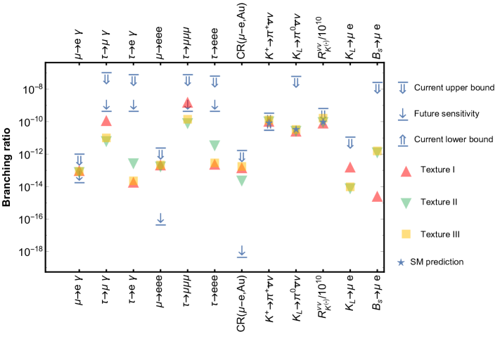
Figure 4: Contributions to several leptonic and mesonic observables associated with the three textures I, II, and III for the benchmark choice $(\epsilon,m_{h_{1}})=(0.215,1.5~{}\text{TeV})$: $\mu\to e\gamma$, $\tau\to\mu\gamma$, $\tau\to e\gamma$, $\mu\to 3e$, $\tau\to 3\mu$, $\mu-e$ conversion, $K^{+}(K_{L})\to\pi^{+}(\pi^{0})\nu\bar{\nu}$, $R^{\nu\nu}_{K^{(\ast)}}/10^{10}$, $B_{s}\to\mu e$, and $K_{L}\to\mu e$. The relevant experimental bounds (and future sensitivities), as well as SM predictions (when appropriate), are also displayed.

Before proceeding, we briefly comment on the other LFUV observables discussed in Section 5.2. The present leptoquark construction leads to SM-like predictions to the distinct $R_{D^{(\ast)}}$ ratios (independently of the texture type and/or mass regime for the exchanged pseudoscalar). If on the one hand this means that, once the distinct experimental constraints have been taken into account, the muon to electron ratios $R_{D^{(\ast)}}^{\mu/e}$ are consistent with experimental measurements, on the other hand it also implies that the current experimental measurement of $R_{D^{(\ast)}}$ (tau to muon ratio, exhibiting a significant deviation from SM predictions) cannot be accounted for. Should the latter $R_{D^{(\ast)}}$ discrepancy be confirmed in the future, then the present leptoquark construction will be ruled out, at least in this minimal version.

8.2 Constraining the leptoquark parameter space

The previously chosen textures, as well as the numerical results (both for the $\epsilon$ parameter and for the contributions to the distinct observables) were obtained for a benchmark value of the $h_{1}$ leptoquark mass, $m_{h_{1}}=1.5$ TeV. The natural question to address is how the viability of the model is impacted by different choices of its parameters, in particular the entries of the $y$ couplings and $m_{h_{1}}$.

To explain the $R_{K^{(*)}}$ anomalies, the BSM construction must comply with the conditions given in Section 5.1, in particular with the interval for the $C^{ee,\mu\mu}_{9,\text{NP}}$ couplings given in Eq. (39); this can also be written as a condition on the ratio of the relevant Yukawa couplings to the $h_{1}$ leptoquark mass, $0.64\times 10^{-3}\lesssim\tfrac{{\rm\,Re}[y_{b\mu}y_{s\mu}^{\ast}-y_{be}y_{se}^{\ast}]}{(m_{h_{1}}/1{\rm~{}TeV})^{2}}\lesssim 1.12\times 10^{-3}$.

Varying the mass of the $h_{1}$ leptoquark over a wide interval - in agreement with LHC direct search bounds - leads to new ranges for the relevant entries of the Yukawa couplings $y_{ij}$ (and thus new values for $\epsilon$). Since for increasing values of $m_{h_{1}}$ saturating the $R_{K^{(*)}}$ anomalies calls for larger $y_{22,32}$ - and hence for larger $\epsilon$ -, bounds on other observables are expected to become more severe, leading to the exclusion of a given realisation. This is displayed on the distinct panels of Fig. 5: the coloured regions denote the contributions for a given observable arising from varying $\epsilon$ (i.e., $y_{ij}$) in the $R_{K^{(*)}}$ favoured interval given above. Light (dark) regions correspond to allowed (excluded) regimes in view of current experimental bounds.

Leading to Fig. 5 we have elected to plot only the most constraining observables: BR($\mu\to e\gamma$), BR($\mu\to 3e$), CR($\mu-e$, Au) and BR($K^{+}\to\pi^{+}\nu\bar{\nu}$). Concerning textures of type I and II, one can verify that CR($\mu-e$, Au) precludes values of the leptoquark mass respectively larger than $m_{h_{1}}\gtrsim 1.8$ TeV and 3.4 TeV (for $\epsilon_{\text{max}}$) and $m_{h_{1}}\gtrsim 3$ TeV and 4.2 TeV (for $\epsilon_{\text{min}}$). (Notice that for texture II $\mu\to 3e$ is almost as constraining as $\mu-e$ conversion in nuclei.) For type III textures, one finds two intervals for $m_{h_{1}}$: [1.75 TeV, 2.75 TeV] and [8 TeV, 11.4 TeV] (the lower and upper bounds obtained in association with the maximal and minimal values of $\epsilon$).

     

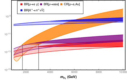
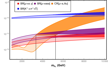
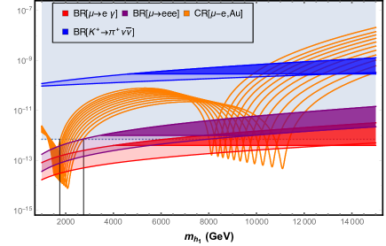
Figure 5: Contributions to BR($\mu\to e\gamma$), BR($\mu\to 3e$), CR($\mu-e$, Au) and BR($K^{+}\to\pi^{+}\nu\bar{\nu}$) as a function of the $h_{1}$ leptoquark mass $m_{h_{1}}$, for type I, II and III textures of $y$ (respectively from left to right, top to bottom), complying with the current interval for $R_{K^{(*)}}$. Light (solid) surfaces denote currently allowed (excluded) regimes due to the violation of the associated experimental bound.

Despite being manifest in all panels, the “kinks” associated with the contributions to CR($\mu-e$, Au) are particularly apparent for type III textures. The behaviour has been well identified in the literature (see, e.g. [159]), and stems from having a localised cancellation of opposite sign up- and down-type quark contributions to the conversion rate (due to different charge and weak isospin).

At this point, it is important to recall that the proposed parametrisation for $y$, as given in Eq. (86), allows each element to be weighed by a real coefficient $a_{ij}$, $\mathcal{O}(1)$. In order to understand how generic perturbations of the unconstrained entries of $y$ affect the phenomenological viability of the model, we have thus taken a type I texture for $y$, and varied one $a_{ij}$ at a time in the range [0.4, 1.6] (with a step size of 0.1). Although not explicitly displayed here, the numerical studies revealed that $\mu\to e\gamma$ and $\mu\to 3e$ are predominantly sensitive to $y_{31}$ ($a_{31}$), with a mild secondary dependence on $y_{21}$ ($a_{21}$); likewise, $\tau\to\mu\gamma$ and $\tau\to 3\mu$ are controlled by $y_{33}$ ($a_{33}$); $\tau\to e\gamma$ and $\tau\to 3e$ are sensitive to variations from both $y_{31}$ and $y_{33}$. Finally, $K^{+}\to\pi^{+}\nu\bar{\nu}$ exhibits a significant dependence on $y_{13}$ ($a_{13}$), $y_{21}$ ($a_{21}$) and $y_{23}$ ($a_{23}$). As a general qualitative statement, for all the radiative and 3-body decays mentioned above, the variation of the $a_{ij}$ coefficients in the interval [0.4, 1.6] leads to a variation of about one order of magnitude in the prediction for the observable. Occurring at the tree level, the neutrinoless $\mu-e$ conversion strongly depends on $y_{11}$ ($a_{11}$), $y_{12}$ ($a_{12}$), and $y_{21}$ ($a_{21}$) - the dominant element depending to a certain extent on the leptoquark mass regime.

The same study can be carried for type II and III textures, with the results reflecting the relative $\epsilon^{n_{ij}}$ dependence.

8.3 Final constraints from neutrino oscillation data

The requirements of having a viable DM candidate, and of accounting for the $R_{K}^{(*)}$ anomalies while complying with all available data on meson and lepton rare decays and transitions have allowed to identify viable flavour textures for the $y$ leptoquark Yukawa couplings, as well as mass regimes for the new states.

As mentioned in Section 3, once the flavour structure of $y$ has been fixed (be it from theoretical arguments or, as in the present case, from a comprehensive phenomenological analysis), the modified Casas-Ibarra parametrisation of Eq. (22) readily allows to determine $\tilde{y}$, while complying with current neutrino oscillation data. As a final step in our study, we thus consider the three textures already discussed in the previous section, and for each one we vary the $n_{ij}$ powers of $\epsilon$ in agreement with the ranges given in Table 5, as well as the associated $a_{ij}$ prefactors (in the range [0.4,1.6]). The $h_{1}$ leptoquark mass is, for simplicity, set to the benchmark value of 1.5 TeV (although the results here discussed qualitatively hold for other choices - in agreement with the discussion of the previous subsection).

Concerning neutrino data, we use the best-fit values from the global oscillation analysis of [160], taking a normal ordering for the neutrino spectrum, with the lightest neutrino mass taken in the range $[10^{-8}~{}\text{eV},0.001~{}\text{eV}]$. As already mentioned, we take the right-handed triplet masses to be $m_{\Sigma}$=2.45, 3.5 and 4.5 TeV. The remaining degrees of freedom in the modified Casas-Ibarra parametrisation are randomly sampled from the following intervals: $[0,2\pi]$ for the phases, and $[-4\pi,4\pi]$ for the angles; one further has $\lambda_{h}\lesssim 4\pi$ (see Eq. (2)).

Each of the thus obtained couplings ($y$ and $\tilde{y}$) are again subject to the various flavour constraints previously discussed; moreover, each entry of the couplings must comply with perturbativity requirements, $|{y}(\tilde{y})|\lesssim 4\pi$.

In order to illustrate our findings, we display in Fig. 6 the results of the scan, for the three types of textures. Since neutrinoless conversion in nuclei and the $K^{+}\to\pi^{+}\nu\bar{\nu}$ decay are the most constraining observables, we display the corresponding predictions of the randomly sampled textures in the plane spanned by the latter two observables; the colour code distinguishes between perturbative and non-perturbative entries of the $y$ and $\tilde{y}$ couplings.

   

Figure 6: Predictions for CR($\mu-e$, N) and BR($K^{+}\to\pi^{+}\nu\bar{\nu}$) associated with randomly sampled $y$ and $\tilde{y}$ (see text), for type I, II and III textures (top to bottom, left to right). The horizontal/vertical lines denote the current experimental bounds, and the colour code identifies perturbative (blue) or non-perturbative (red) regimes of $\tilde{y}$.

As is manifest from inspection of Fig. 6, accommodating $\nu$-oscillation data from type I textures for the leptoquark $y$ couplings, in agreement with experimental data, and for perturbative $\tilde{y}$ does not excessively constrain the remaining degrees of freedom. Even though perturbative regimes for $\tilde{y}$ are more likely to be associated with large values of BR($K^{+}\to\pi^{+}\nu\bar{\nu}$), one can easily find regimes which are phenomenologically allowed. Notice however that a near-future improvement in the associated experimental sensitivities (for instance CR($\mu-e$, Al)$~{}\sim 10^{-15}$, and BR($K^{+}\to\pi^{+}\nu\bar{\nu}$)$\sim 10^{-10}$) should allow to probe the present leptoquark construction (and possibly falsify it).

For type II textures, the associated panel of Fig. 6 reveals that perturbative $\tilde{y}$ couplings are far harder to accommodate, especially due to the excessive contributions to CR($\mu-e$, Au). Finally, notice that only a tiny subset of the sampled type III textures is in agreement with flavour observables, and no sub-region of the latter leads to perturbative $\tilde{y}$. One thus concludes that type III textures (despite being marginally compatible with all the quark and lepton observables here discussed) do not lead to a satisfactory leptoquark construction.

We have also explored the possibility of having a distinct ordering (inverted) for the light neutrino spectrum: in what concerns type I textures, we found no significant changes, so that in fact both orderings can be easily accommodated; in the case of type II textures for $y$ (which do allow to accommodate oscillation data for a normal ordering) we failed to find viable solutions for an inverted ordering; finally, type III textures remain unable to account for oscillation data with perturbative values of the couplings even in the case of a inverted ordering of the neutrino spectrum.

Before moving to our final remarks, it is worth mentioning that it would have been theoretically appealing to have FN-inspired textures for both $y$ and $\tilde{y}$ couplings; as can be indirectly inferred from the above discussion, we did not succeed in finding phenomenologically viable $\tilde{y}$ couplings with textures mirroring those of $y$.

9 Concluding remarks

In this work we have carried a comprehensive phenomenological study of a SM extension via two scalar leptoquarks $h_{1,2}$ and three generations of triplet neutrinos $\Sigma_{R}^{i}$, further reinforcing the SM gauge group via a discrete $Z_{2}$ symmetry under which $h_{2}$ and $\Sigma_{R}^{i}$ are odd (all other fields being even).

The present New Physics construction aims at simultaneously addressing two long-standing SM observational problems - neutrino mass generation, and a viable dark matter candidate - while further offering a solution to the currently reported anomalies in $B$ meson decays, $R_{K^{(*)}}$.

The $Z_{2}$ symmetry ensures the stability of the LZoP, rendering the neutral component of the lightest $\Sigma_{R}$ a viable cold dark matter candidate for well defined intervals of its mass. In the absence of a full theory of flavour, we have identified several classes of flavour textures for the $h_{1}$ leptoquark Yukawa couplings which succeed in saturating the $R_{K^{(*)}}$ anomalies. These textures (loosely based on Froggatt-Nielsen inspired ansätze) were subjected to a vast array of flavour conserving and flavour violating observables (including meson decays, neutral meson oscillations and cLFV decays), which allowed to infer stringent constraints on the $h_{1}$ leptoquark mass and couplings. Contrary to previous claims in the literature, our findings suggest that the strongest constraints on these leptoquark extensions do arise from cLFV $\mu-e$ conversion in nuclei, and from the rare $K^{+}\to\pi^{+}\nu\bar{\nu}$ decays. Furthermore, we also verified that numerous ansätze (identified as promising ones for leptoquarks couplings, see e.g. [74, 75]) were in fact phenomenologically disfavoured by several of the here considered observables.

It is important to emphasise that the constraints on leptoquark couplings arising from flavour observables are not intrinsic (nor peculiar) to the leptoquark realisation here considered; in fact these are valid for any SM extension via scalar triplet leptoquarks.

The present BSM realisation leads to a scenario in which neutrino masses are radiatively generated (at the three-loop level, from the exchange of leptoquarks, down-type quarks and lepton triplets, see Fig. 1). Neutrino oscillation data can be accounted for by means of a modified Casas-Ibarra parametrisation: avoiding non-perturbative regimes for the Yukawa couplings, $y$ and $\tilde{y}$, establishes the final constraints on the parameter space of the model.

The inclusion of Majorana states opens the door to lepton number violating processes; the radiatively induced masses for the light (left-handed) neutrinos are one such example. The new interactions and couplings further allow for additional sources of CP violation. It is thus only natural to envisage the possibility of accounting for the baryon asymmetry of the universe. In the present realisation, one can have tree-level processes which are lepton number violating: one such example can be obtained from the neutrino mass (loop) diagrams - see Fig. 1 -, by “cutting” the inner fermion propagators. This would lead to tree-level LNV decays of the heavier neutral $\Sigma^{2,0}_{R}$ into, for instance, $\Sigma^{1,0}_{R}+\bar{d}+\bar{d}+d\nu_{L}+d\nu_{L}$ (which could have CP violating interferences with higher order diagrams). However, these appear to be heavily suppressed processes and, in the absence of a detailed evaluation, it remains unclear whether one could indeed generate a significant lepton asymmetry. In addition, $\Sigma_{R}$ decoupling would be required to occur above the EW phase transition to have an efficient conversion into a baryon asymmetry.

In summary, and following a thorough study of an extensive array of observables, we have proposed realisations of a SM scalar leptoquark extension capable of accommodating neutrino oscillation data, a viable DM candidate, and saturating the observed discrepancies for $R_{K^{(*)}}$. We notice that the present construction cannot account for the tensions in $R_{D^{(*)}}$, nor for the discrepancy between observation and SM prediction in what concerns the muon anomalous magnetic moment. Should the latter persist, then the candidate model here studied will have to be extended, or then embedded in a larger framework [62].

In the near future, a number of high-intensity experiments will put the present leptoquark construction to the test, in particular several cLFV-dedicated facilities (searches for radiative and three-body muon decays, in addition to neutrinoless conversion in nuclei) and a possible measurement of the rare decay $K^{+}\to\pi^{+}\nu\bar{\nu}$. Hopefully, positive signals or new stringent bounds emerging from negative searches, will allow to further constrain the model’s parameter space, or possibly disfavour it as a candidate New Physics model.

References

• [1] C. Patrignani et al. [Particle Data Group], Chin. Phys. C 40, no. 10, 100001 (2016).
• [2] G. Hiller and F. Kruger, Phys. Rev. D 69, 074020 (2004) [hep-ph/0310219].
• [3] R. Aaij et al. [LHCb Collaboration], Phys. Rev. Lett.  113, 151601 (2014) [arXiv:1406.6482 [hep-ex]].
• [4] M. Bordone, G. Isidori and A. Pattori, Eur. Phys. J. C 76, no. 8, 440 (2016) [arXiv:1605.07633 [hep-ph]].
• [5] B. Capdevila, A. Crivellin, S. Descotes-Genon, J. Matias and J. Virto, JHEP 1801, 093 (2018) [arXiv:1704.05340 [hep-ph]].
• [6] R. Aaij et al. [LHCb Collaboration], JHEP 1708, 055 (2017) [arXiv:1705.05802 [hep-ex]].
• [7] http://www.slac.stanford.edu/xorg/hflav/semi/fpcp17/RDRDs.html
• [8] J. P. Lees et al. [BaBar Collaboration], Phys. Rev. Lett.  109, 101802 (2012) [arXiv:1205.5442 [hep-ex]].
• [9] J. P. Lees et al. [BaBar Collaboration], Phys. Rev. D 88, no. 7, 072012 (2013) [arXiv:1303.0571 [hep-ex]].
• [10] M. Huschle et al. [Belle Collaboration], Phys. Rev. D 92, no. 7, 072014 (2015) [arXiv:1507.03233 [hep-ex]].
• [11] I. Adachi et al. [Belle Collaboration], arXiv:0910.4301 [hep-ex].
• [12] A. Bozek et al. [Belle Collaboration], Phys. Rev. D 82, 072005 (2010) [arXiv:1005.2302 [hep-ex]].
• [13] R. Aaij et al. [LHCb Collaboration], Phys. Rev. Lett.  115, no. 11, 111803 (2015) Erratum: [Phys. Rev. Lett.  115, no. 15, 159901 (2015)] [arXiv:1506.08614 [hep-ex]].
• [14] S. Hirose et al. [Belle Collaboration], Phys. Rev. Lett.  118, no. 21, 211801 (2017) [arXiv:1612.00529 [hep-ex]].
• [15] D. Bigi and P. Gambino, Phys. Rev. D 94, no. 9, 094008 (2016) [arXiv:1606.08030 [hep-ph]].
• [16] Y. Amhis et al. [HFLAV Collaboration], Eur. Phys. J. C 77, no. 12, 895 (2017) [arXiv:1612.07233 [hep-ex]].
• [17] D. Bigi, P. Gambino and S. Schacht, JHEP 1711, 061 (2017) [arXiv:1707.09509 [hep-ph]].
• [18] Z. Ligeti, M. Papucci and D. J. Robinson, JHEP 1701, 083 (2017) [arXiv:1610.02045 [hep-ph]].
• [19] A. Crivellin, J. Fuentes-Martin, A. Greljo and G. Isidori, Phys. Lett. B 766, 77 (2017) [arXiv:1611.02703 [hep-ph]].
• [20] B. Capdevila, S. Descotes-Genon, L. Hofer and J. Matias, JHEP 1704, 016 (2017) [arXiv:1701.08672 [hep-ph]].
• [21] S. Wehle et al. [Belle Collaboration], Phys. Rev. Lett.  118, no. 11, 111801 (2017) [arXiv:1612.05014 [hep-ex]].
• [22] A. Datta, M. Duraisamy and D. Ghosh, Phys. Rev. D 89, no. 7, 071501 (2014) [arXiv:1310.1937 [hep-ph]].
• [23] D. Ghosh, M. Nardecchia and S. A. Renner, JHEP 1412, 131 (2014) [arXiv:1408.4097 [hep-ph]].
• [24] S. L. Glashow, D. Guadagnoli and K. Lane, Phys. Rev. Lett.  114, 091801 (2015) [arXiv:1411.0565 [hep-ph]].
• [25] B. Bhattacharya, A. Datta, D. London and S. Shivashankara, Phys. Lett. B 742, 370 (2015) [arXiv:1412.7164 [hep-ph]].
• [26] M. Freytsis, Z. Ligeti and J. T. Ruderman, Phys. Rev. D 92, no. 5, 054018 (2015) [arXiv:1506.08896 [hep-ph]].
• [27] D. Bardhan, P. Byakti and D. Ghosh, JHEP 1701, 125 (2017) [arXiv:1610.03038 [hep-ph]].
• [28] D. Ghosh, Eur. Phys. J. C 77, no. 10, 694 (2017) [arXiv:1704.06240 [hep-ph]].
• [29] M. Ciuchini, A. M. Coutinho, M. Fedele, E. Franco, A. Paul, L. Silvestrini and M. Valli, Eur. Phys. J. C 77, no. 10, 688 (2017) [arXiv:1704.05447 [hep-ph]].
• [30] D. Choudhury, A. Kundu, R. Mandal and R. Sinha, Phys. Rev. Lett.  119, no. 15, 151801 (2017) [arXiv:1706.08437 [hep-ph]].
• [31] D. Choudhury, A. Kundu, R. Mandal and R. Sinha, arXiv:1712.01593 [hep-ph].
• [32] W. Altmannshofer, S. Gori, M. Pospelov and I. Yavin, Phys. Rev. D 89, 095033 (2014) [arXiv:1403.1269 [hep-ph]].
• [33] A. Crivellin, G. D’Ambrosio and J. Heeck, Phys. Rev. Lett.  114, 151801 (2015) [arXiv:1501.00993 [hep-ph]].
• [34] A. Crivellin, G. D’Ambrosio and J. Heeck, Phys. Rev. D 91, no. 7, 075006 (2015) [arXiv:1503.03477 [hep-ph]].
• [35] D. Aristizabal Sierra, F. Staub and A. Vicente, Phys. Rev. D 92, no. 1, 015001 (2015) [arXiv:1503.06077 [hep-ph]].
• [36] A. Crivellin, L. Hofer, J. Matias, U. Nierste, S. Pokorski and J. Rosiek, Phys. Rev. D 92, no. 5, 054013 (2015) [arXiv:1504.07928 [hep-ph]].
• [37] A. Celis, J. Fuentes-Martin, M. Jung and H. Serodio, Phys. Rev. D 92, no. 1, 015007 (2015) [arXiv:1505.03079 [hep-ph]].
• [38] D. Bhatia, S. Chakraborty and A. Dighe, JHEP 1703, 117 (2017) [arXiv:1701.05825 [hep-ph]].
• [39] J. F. Kamenik, Y. Soreq and J. Zupan, Phys. Rev. D 97, no. 3, 035002 (2018) [arXiv:1704.06005 [hep-ph]].
• [40] J. E. Camargo-Molina, A. Celis and D. A. Faroughy, arXiv:1805.04917 [hep-ph].
• [41] G. Hiller and M. Schmaltz, Phys. Rev. D 90, 054014 (2014) [arXiv:1408.1627 [hep-ph]].
• [42] B. Gripaios, M. Nardecchia and S. A. Renner, JHEP 1505, 006 (2015) [arXiv:1412.1791 [hep-ph]].
• [43] S. Sahoo and R. Mohanta, Phys. Rev. D 91, no. 9, 094019 (2015) [arXiv:1501.05193 [hep-ph]].
• [44] I. de Medeiros Varzielas and G. Hiller, JHEP 1506, 072 (2015) [arXiv:1503.01084 [hep-ph]].
• [45] R. Alonso, B. Grinstein and J. Martin Camalich, JHEP 1510, 184 (2015) [arXiv:1505.05164 [hep-ph]].
• [46] M. Bauer and M. Neubert, Phys. Rev. Lett.  116, no. 14, 141802 (2016) [arXiv:1511.01900 [hep-ph]].
• [47] C. Hati, G. Kumar and N. Mahajan, JHEP 1601, 117 (2016) [arXiv:1511.03290 [hep-ph]].
• [48] S. Fajfer and N. Košnik, Phys. Lett. B 755, 270 (2016) [arXiv:1511.06024 [hep-ph]].
• [49] D. Das, C. Hati, G. Kumar and N. Mahajan, Phys. Rev. D 94, 055034 (2016) [arXiv:1605.06313 [hep-ph]].
• [50] D. Bečirević, S. Fajfer, N. Kosnik and O. Sumensari, Phys. Rev. D 94, no. 11, 115021 (2016) [arXiv:1608.08501 [hep-ph]].
• [51] S. Sahoo, R. Mohanta and A. K. Giri, Phys. Rev. D 95, no. 3, 035027 (2017) [arXiv:1609.04367 [hep-ph]].
• [52] P. Cox, A. Kusenko, O. Sumensari and T. T. Yanagida, JHEP 1703, 035 (2017) [arXiv:1612.03923 [hep-ph]].
• [53] A. Crivellin, D. Müller and T. Ota, JHEP 1709, 040 (2017) [arXiv:1703.09226 [hep-ph]].
• [54] D. Bečirević and O. Sumensari, JHEP 1708, 104 (2017) [arXiv:1704.05835 [hep-ph]].
• [55] Y. Cai, J. Gargalionis, M. A. Schmidt and R. R. Volkas, JHEP 1710, 047 (2017) [arXiv:1704.05849 [hep-ph]].
• [56] D. Buttazzo, A. Greljo, G. Isidori and D. Marzocca, JHEP 1711, 044 (2017) [arXiv:1706.07808 [hep-ph]].
• [57] I. Doršner, S. Fajfer, D. A. Faroughy and N. Košnik, JHEP 1710, 188 (2017) [arXiv:1706.07779 [hep-ph]].
• [58] M. Blanke and A. Crivellin, arXiv:1801.07256 [hep-ph].
• [59] A. Greljo and B. A. Stefanek, Phys. Lett. B 782, 131 (2018) [arXiv:1802.04274 [hep-ph]].
• [60] M. Bordone, C. Cornella, J. Fuentes-Martin and G. Isidori, arXiv:1805.09328 [hep-ph].
• [61] S. Sahoo and R. Mohanta, arXiv:1806.01048 [hep-ph].
• [62] D. Bečirević, I. Doršner, S. Fajfer, N. Košnik, D. A. Faroughy and O. Sumensari, arXiv:1806.05689 [hep-ph].
• [63] A. Greljo, G. Isidori and D. Marzocca, JHEP 1507, 142 (2015) [arXiv:1506.01705 [hep-ph]].
• [64] P. Arnan, D. Bečirević, F. Mescia and O. Sumensari, Eur. Phys. J. C 77, no. 11, 796 (2017) [arXiv:1703.03426 [hep-ph]].
• [65] L. S. Geng, B. Grinstein, S. Jäger, J. Martin Camalich, X. L. Ren and R. X. Shi, Phys. Rev. D 96, no. 9, 093006 (2017) [arXiv:1704.05446 [hep-ph]].
• [66] W. Altmannshofer, P. S. Bhupal Dev and A. Soni, Phys. Rev. D 96, no. 9, 095010 (2017) [arXiv:1704.06659 [hep-ph]].
• [67] D. Das, C. Hati, G. Kumar and N. Mahajan, Phys. Rev. D 96, no. 9, 095033 (2017) [arXiv:1705.09188 [hep-ph]].
• [68] K. Earl and T. Gregoire, arXiv:1806.01343 [hep-ph].
• [69] Y. Cai, J. Herrero-García, M. A. Schmidt, A. Vicente and R. R. Volkas, Front. in Phys.  5, 63 (2017) [arXiv:1706.08524 [hep-ph]].
• [70] F. F. Deppisch, S. Kulkarni, H. Päs and E. Schumacher, Phys. Rev. D 94, no. 1, 013003 (2016) [arXiv:1603.07672 [hep-ph]].
• [71] A. Zee, Nucl. Phys. B 264, 99 (1986).
• [72] K. S. Babu, Phys. Lett. B 203, 132 (1988).
• [73] S. Y. Guo, Z. L. Han, B. Li, Y. Liao and X. D. Ma, Nucl. Phys. B 928, 435 (2018) [arXiv:1707.00522 [hep-ph]].
• [74] T. Nomura, H. Okada and N. Okada, Phys. Lett. B 762, 409 (2016) [arXiv:1608.02694 [hep-ph]].
• [75] K. Cheung, T. Nomura and H. Okada, Phys. Rev. D 95, no. 1, 015026 (2017) [arXiv:1610.04986 [hep-ph]].
• [76] L. M. Krauss, S. Nasri and M. Trodden, Phys. Rev. D 67, 085002 (2003) [hep-ph/0210389].
• [77] R. Foot, H. Lew, X. G. He and G. C. Joshi, Z. Phys. C 44, 441 (1989).
• [78] C. S. Chen, K. L. McDonald and S. Nasri, Phys. Lett. B 734, 388 (2014) [arXiv:1404.6033 [hep-ph]].
• [79] I. Dorsner, S. Fajfer, J. F. Kamenik and N. Kosnik, Phys. Lett. B 682, 67 (2009) [arXiv:0906.5585 [hep-ph]].
• [80] C. Hati and U. Sarkar, arXiv:1805.06081 [hep-ph].
• [81] A. Ahriche and S. Nasri, JCAP 1307, 035 (2013) [arXiv:1304.2055 [hep-ph]].
• [82] G. Passarino and M. J. G. Veltman, Nucl. Phys. B 160, 151 (1979).
• [83] J. A. Casas and A. Ibarra, Nucl. Phys. B 618, 171 (2001) [hep-ph/0103065].
• [84] M. Cirelli, N. Fornengo and A. Strumia, Nucl. Phys. B 753, 178 (2006) [hep-ph/0512090].
• [85] E. Ma and D. Suematsu, Mod. Phys. Lett. A 24, 583 (2009) [arXiv:0809.0942 [hep-ph]].
• [86] K. Griest and D. Seckel, Phys. Rev. D 43, 3191 (1991).
• [87] P. A. R. Ade et al. [Planck Collaboration], Astron. Astrophys.  594, A13 (2016) [arXiv:1502.01589 [astro-ph.CO]].
• [88] S. Choubey, S. Khan, M. Mitra and S. Mondal, Eur. Phys. J. C 78, no. 4, 302 (2018) [arXiv:1711.08888 [hep-ph]].
• [89] W. Altmannshofer, P. Ball, A. Bharucha, A. J. Buras, D. M. Straub and M. Wick, JHEP 0901, 019 (2009) [arXiv:0811.1214 [hep-ph]].
• [90] D. Bečirević, N. Košnik, O. Sumensari and R. Zukanovich Funchal, JHEP 1611, 035 (2016) [arXiv:1608.07583 [hep-ph]].
• [91] G. Hiller and I. Nisandzic, Phys. Rev. D 96, no. 3, 035003 (2017) [arXiv:1704.05444 [hep-ph]].
• [92] S. Descotes-Genon, L. Hofer, J. Matias and J. Virto, JHEP 1606, 092 (2016) [arXiv:1510.04239 [hep-ph]].
• [93] T. Hurth, F. Mahmoudi and S. Neshatpour, JHEP 1412, 053 (2014) [arXiv:1410.4545 [hep-ph]].
• [94] W. Altmannshofer and D. M. Straub, Eur. Phys. J. C 75, no. 8, 382 (2015) [arXiv:1411.3161 [hep-ph]].
• [95] F. Beaujean, C. Bobeth and D. van Dyk, Eur. Phys. J. C 74, 2897 (2014) Erratum: [Eur. Phys. J. C 74, 3179 (2014)] [arXiv:1310.2478 [hep-ph]].
• [96] R. Glattauer et al. [Belle Collaboration], Phys. Rev. D 93, no. 3, 032006 (2016) [arXiv:1510.03657 [hep-ex]].
• [97] A. Abdesselam et al. [Belle Collaboration], arXiv:1702.01521 [hep-ex].
• [98] A. J. Buras, D. Buttazzo, J. Girrbach-Noe and R. Knegjens, JHEP 1511, 033 (2015) [arXiv:1503.02693 [hep-ph]].
• [99] A. V. Artamonov et al. [E949 Collaboration], Phys. Rev. Lett.  101, 191802 (2008) [arXiv:0808.2459 [hep-ex]].
• [100] NA62 Collaboration, Contribution to the ”53rd Rencontres de Moriond on Electroweak Interactions and Unified Theories (Moriond EW 2018)”, La Thuile, Italy, 10-17 March 2018.
• [101] J. K. Ahn et al. [E391a Collaboration], Phys. Rev. D 81, 072004 (2010) [arXiv:0911.4789 [hep-ex]].
• [102] J. Grygier et al. [Belle Collaboration], Phys. Rev. D 96, no. 9, 091101 (2017) [arXiv:1702.03224 [hep-ex]].
• [103] J. Charles et al., Phys. Rev. D 91, no. 7, 073007 (2015) [arXiv:1501.05013 [hep-ph]].
• [104] J. Brod and M. Gorbahn, Phys. Rev. Lett.  108, 121801 (2012) [arXiv:1108.2036 [hep-ph]].
• [105] A. Crivellin, G. D’Ambrosio, M. Hoferichter and L. C. Tunstall, Phys. Rev. D 93, no. 7, 074038 (2016) [arXiv:1601.00970 [hep-ph]].
• [106] S. Fajfer, N. Košnik and L. Vale Silva, Eur. Phys. J. C 78, no. 4, 275 (2018) [arXiv:1802.00786 [hep-ph]].
• [107] A. J. Buras, J. Girrbach-Noe, C. Niehoff and D. M. Straub, JHEP 1502, 184 (2015) [arXiv:1409.4557 [hep-ph]].
• [108] C. Bobeth and A. J. Buras, JHEP 1802, 101 (2018) [arXiv:1712.01295 [hep-ph]].
• [109] M. Bordone, D. Buttazzo, G. Isidori and J. Monnard, Eur. Phys. J. C 77, no. 9, 618 (2017) [arXiv:1705.10729 [hep-ph]].
• [110] G. Buchalla and A. J. Buras, Nucl. Phys. B 400, 225 (1993).
• [111] M. Misiak and J. Urban, Phys. Lett. B 451, 161 (1999) [hep-ph/9901278].
• [112] G. Buchalla and A. J. Buras, Nucl. Phys. B 548, 309 (1999) [hep-ph/9901288].
• [113] J. Brod, M. Gorbahn and E. Stamou, Phys. Rev. D 83, 034030 (2011) [arXiv:1009.0947 [hep-ph]].
• [114] G. Buchalla and A. J. Buras, Nucl. Phys. B 412, 106 (1994) [hep-ph/9308272].
• [115] A. J. Buras, M. Gorbahn, U. Haisch and U. Nierste, Phys. Rev. Lett.  95, 261805 (2005) [hep-ph/0508165].
• [116] A. J. Buras, M. Gorbahn, U. Haisch and U. Nierste, JHEP 0611, 002 (2006) Erratum: [JHEP 1211, 167 (2012)] [hep-ph/0603079].
• [117] G. Isidori, F. Mescia and C. Smith, Nucl. Phys. B 718, 319 (2005) [hep-ph/0503107].
• [118] A. Lenz et al., Phys. Rev. D 83, 036004 (2011) [arXiv:1008.1593 [hep-ph]].
• [119] M. Bona et al. [UTfit Collaboration], JHEP 0803, 049 (2008) [arXiv:0707.0636 [hep-ph]]; New Physics Fit results: Summer 2016, http://www.utfit.org/UTfit/ResultsSummer2016NP.
• [120] T. Inami and C. S. Lim, Prog. Theor. Phys.  65, 297 (1981) Erratum: [Prog. Theor. Phys.  65, 1772 (1981)].
• [121] A. J. Buras, hep-ph/9806471.
• [122] A. J. Buras, M. Jamin and P. H. Weisz, Nucl. Phys. B 347, 491 (1990).
• [123] J. Brod and M. Gorbahn, Phys. Rev. D 82, 094026 (2010) [arXiv:1007.0684 [hep-ph]].
• [124] A. J. Buras, JHEP 1604, 071 (2016) [arXiv:1601.00005 [hep-ph]].
• [125] A. J. Buras, F. De Fazio, J. Girrbach and M. V. Carlucci, JHEP 1302, 023 (2013) [arXiv:1211.1237 [hep-ph]].
• [126] A. J. Buras, J. M. Gérard and W. A. Bardeen, Eur. Phys. J. C 74, 2871 (2014) [arXiv:1401.1385 [hep-ph]].
• [127] V. Khachatryan et al. [CMS and LHCb Collaborations], Nature 522, 68 (2015) [arXiv:1411.4413 [hep-ex]].
• [128] M. Aaboud et al. [ATLAS Collaboration], Eur. Phys. J. C 76, no. 9, 513 (2016) [arXiv:1604.04263 [hep-ex]].
• [129] D. Bečirević, O. Sumensari and R. Zukanovich Funchal, Eur. Phys. J. C 76, no. 3, 134 (2016) [arXiv:1602.00881 [hep-ph]].
• [130] G. D’Ambrosio, G. Isidori and J. Portoles, Phys. Lett. B 423, 385 (1998) [hep-ph/9708326].
• [131] A. M. Baldini et al. [MEG Collaboration], Eur. Phys. J. C 76, no. 8, 434 (2016) [arXiv:1605.05081 [hep-ex]].
• [132] A. M. Baldini et al. [MEG II Collaboration], Eur. Phys. J. C 78, no. 5, 380 (2018) [arXiv:1801.04688 [physics.ins-det]].
• [133] G. Cavoto, A. Papa, F. Renga, E. Ripiccini and C. Voena, Eur. Phys. J. C 78, no. 1, 37 (2018) [arXiv:1707.01805 [hep-ex]].
• [134] B. Aubert et al. [BaBar Collaboration], Phys. Rev. Lett.  104, 021802 (2010) [arXiv:0908.2381 [hep-ex]].
• [135] T. Aushev et al., arXiv:1002.5012 [hep-ex].
• [136] U. Bellgardt et al. [SINDRUM Collaboration], Nucl. Phys. B 299, 1 (1988).
• [137] A. Blondel et al., arXiv:1301.6113 [physics.ins-det].
• [138] K. Hayasaka et al., Phys. Lett. B 687, 139 (2010) [arXiv:1001.3221 [hep-ex]].
• [139] W. H. Bertl et al. [SINDRUM II Collaboration], Eur. Phys. J. C 47, 337 (2006).
• [140] T. M. Nguyen [DeeMe Collaboration], PoS FPCP 2015, 060 (2015).
• [141] B. E. Krikler [COMET Collaboration], arXiv:1512.08564 [physics.ins-det].
• [142] L. Bartoszek et al. [Mu2e Collaboration], arXiv:1501.05241 [physics.ins-det].
• [143] Y. Kuno, Nucl. Phys. Proc. Suppl.  149, 376 (2005).
• [144] I. Doršner, S. Fajfer, A. Greljo, J. F. Kamenik and N. Košnik, Phys. Rept.  641, 1 (2016) [arXiv:1603.04993 [hep-ph]].
• [145] Y. Kuno and Y. Okada, Rev. Mod. Phys.  73, 151 (2001) [hep-ph/9909265].
• [146] Y. Okada, K. i. Okumura and Y. Shimizu, Phys. Rev. D 61, 094001 (2000) [hep-ph/9906446].
• [147] S. Davidson, Y. Kuno and A. Saporta, Eur. Phys. J. C 78, no. 2, 109 (2018) [arXiv:1710.06787 [hep-ph]].
• [148] R. Kitano, M. Koike and Y. Okada, Phys. Rev. D 66, 096002 (2002) Erratum: [Phys. Rev. D 76, 059902 (2007)] [hep-ph/0203110].
• [149] M. Aaboud et al. [ATLAS Collaboration], New J. Phys.  18, no. 9, 093016 (2016) [arXiv:1605.06035 [hep-ex]].
• [150] A. M. Sirunyan et al. [CMS Collaboration], JHEP 1707, 121 (2017) [arXiv:1703.03995 [hep-ex]].
• [151] The ATLAS collaboration [ATLAS Collaboration], ATLAS-CONF-2016-078.
• [152] M. Aaboud et al. [ATLAS Collaboration], Eur. Phys. J. C 76, no. 10, 547 (2016) [arXiv:1606.08772 [hep-ex]].
• [153] C. D. Froggatt and H. B. Nielsen, Nucl. Phys. B 147, 277 (1979).
• [154] A. E. Cárcamo Hernández, I. de Medeiros Varzielas and E. Schumacher, arXiv:1601.00661 [hep-ph].
• [155] A. E. Cárcamo Hernández, I. de Medeiros Varzielas and E. Schumacher, Phys. Rev. D 93, no. 1, 016003 (2016) [arXiv:1509.02083 [hep-ph]].
• [156] A. E. Cárcamo Hernández, Eur. Phys. J. C 76, no. 9, 503 (2016) [arXiv:1512.09092 [hep-ph]].
• [157] M. D. Campos, A. E. Cárcamo Hernández, H. Päs and E. Schumacher, Phys. Rev. D 91, no. 11, 116011 (2015) [arXiv:1408.1652 [hep-ph]].
• [158] R. Barbieri, G. Isidori, A. Pattori and F. Senia, Eur. Phys. J. C 76, no. 2, 67 (2016) [arXiv:1512.01560 [hep-ph]].
• [159] R. Alonso, M. Dhen, M. B. Gavela and T. Hambye, JHEP 1301, 118 (2013) [arXiv:1209.2679 [hep-ph]].
• [160] P. F. de Salas, D. V. Forero, C. A. Ternes, M. Tortola and J. W. F. Valle, Phys. Lett. B 782, 633 (2018) [arXiv:1708.01186 [hep-ph]].