The normalized Laplacian spectra of subdivision vertex-edge neighbourhood vertex(edge)-corona for graphs111This work is supported by the Young Scholars Science Foundation of Lanzhou Jiaotong University (No.2016014) and NSFC (No.11461038).

Fei Wen1,2,   You Zhang2,   Wei Wang1,222E-mail addresses: wang_weiw@163.com(W. Wang), wenfei@mail.lzjtu.cn(F. Wen).
1. School of Mathematics and Statistics, Xi’an Jiaotong University, Xi’an 710049, P.R. China
2. Institute of Applied Mathematics, Lanzhou Jiaotong University, Lanzhou 730070, P.R.China

Abstract.

In this paper, we introduce two new graph operations, namely, the subdivision vertex-edge neighbourhood vertex-corona and the subdivision vertex-edge neighbourhood edge-corona on graphs G1subscript𝐺1G_{1}, G2subscript𝐺2G_{2} and G3subscript𝐺3G_{3}, and the resulting graphs are denoted by G1S(G2VG3E)superscriptsubscript𝐺1𝑆superscriptsubscript𝐺2𝑉superscriptsubscript𝐺3𝐸G_{1}^{S}\bowtie(G_{2}^{V}\cup G_{3}^{E}) and G1S(G2VG3E)superscriptsubscript𝐺1𝑆superscriptsubscript𝐺2𝑉superscriptsubscript𝐺3𝐸G_{1}^{S}\diamondsuit(G_{2}^{V}\cup G_{3}^{E}), respectively. Whereafter, the normalized Laplacian spectra of G1S(G2VG3E)superscriptsubscript𝐺1𝑆superscriptsubscript𝐺2𝑉superscriptsubscript𝐺3𝐸G_{1}^{S}\bowtie(G_{2}^{V}\cup G_{3}^{E}) and G1S(G2VG3E)superscriptsubscript𝐺1𝑆superscriptsubscript𝐺2𝑉superscriptsubscript𝐺3𝐸G_{1}^{S}\diamondsuit(G_{2}^{V}\cup G_{3}^{E}) are respectively determined in terms of the corresponding normalized Laplacian spectra of the connected regular graphs G1subscript𝐺1G_{1}, G2subscript𝐺2G_{2} and G3subscript𝐺3G_{3}, which extend the corresponding results of [A. Das, P. Panigrahi, Linear Multil. Algebra, 2017, 65(5): 962-972]. As applications, these results enable us to construct infinitely many pairs of normalized Laplacian cospectral graphs. Moreover, we also give the number of the spanning trees, the multiplicative degree-Kirchhoff index and Kemeny’s constant of G1S(G2VG3E)superscriptsubscript𝐺1𝑆superscriptsubscript𝐺2𝑉superscriptsubscript𝐺3𝐸G_{1}^{S}\bowtie(G_{2}^{V}\cup G_{3}^{E}) (resp. G1S(G2VG3E)superscriptsubscript𝐺1𝑆superscriptsubscript𝐺2𝑉superscriptsubscript𝐺3𝐸G_{1}^{S}\diamondsuit(G_{2}^{V}\cup G_{3}^{E})).

Keywords

: subdivision vertex-edge neighbourhood vertex-corona, subdivision vertex-edge neighbourhood edge-corona, normalized Laplacian spectrum, cospectral graphs

AMS Classifications

: 05C50

1 Introduction

Throughout this paper, we are concerned only with simple undirected graphs (loops and multiple edges are not allowed). Let G𝐺G be a graph with vertex set V(G)={v1,v2,,vn}𝑉𝐺subscript𝑣1subscript𝑣2subscript𝑣𝑛V(G)=\{v_{1},v_{2},\ldots,v_{n}\} and edge set E(G)={e1,e2,,em}𝐸𝐺subscript𝑒1subscript𝑒2subscript𝑒𝑚E(G)=\{e_{1},e_{2},\ldots,e_{m}\} where |V(G)|=n𝑉𝐺𝑛|V(G)|=n, |E(G)|=m𝐸𝐺𝑚|E(G)|=m. The line graph (G)𝐺\ell(G) of graph G𝐺G is a graph whose vertices corresponding the edges of G𝐺G, and where two vertices are adjacent iff the corresponding edges of G𝐺G are adjacent. We denote the complete graph and the cycle of order n𝑛n by Knsubscript𝐾𝑛K_{n} and Cn(n3)subscript𝐶𝑛𝑛3C_{n}(n\geq 3), respectively. A graph matrix M=M(G)𝑀𝑀𝐺M=M(G) is defined to be a symmetric matrix with respect to adjacency matrix A(G)𝐴𝐺A(G) of G𝐺G. The M𝑀M-characteristic polynomial of G𝐺G is defined as ΦM(x)=det(xIM)subscriptΦ𝑀𝑥𝑥𝐼𝑀\Phi_{M}(x)=\det(xI-M), where I𝐼I is the identity matrix. The M𝑀M-eigenvalues of G𝐺G are the eigenvalues of its M𝑀M-polynomial. The M𝑀M-spectrum, denoted by SpecM(G)𝑆𝑝𝑒subscript𝑐𝑀𝐺Spec_{M}(G), of G𝐺G is a multiset consisting of the M𝑀M-eigenvalues. And two graphs G𝐺G and H𝐻H are M𝑀M–cospectral if ΦM(G)(x)=ΦM(H)(x)subscriptΦ𝑀𝐺𝑥subscriptΦ𝑀𝐻𝑥\Phi_{M(G)}(x)=\Phi_{M(H)}(x).

Let D(G)=diag(dv1,dv2,,dvn)𝐷𝐺𝑑𝑖𝑎𝑔subscript𝑑subscript𝑣1subscript𝑑subscript𝑣2subscript𝑑subscript𝑣𝑛D(G)=diag(d_{v_{1}},d_{v_{2}},\ldots,d_{v_{n}}) be the degree diagonal matrix of G𝐺G. The graph matrix M=M(G)𝑀𝑀𝐺M=M(G) is respectively called the adjacency matrix, the signless Laplacian matrix and the normalized Laplacian matrix of G𝐺G if M𝑀M equals A(G)𝐴𝐺A(G), Q(G)=D(G)+A(G)𝑄𝐺𝐷𝐺𝐴𝐺Q(G)=D(G)+A(G) and (G)=D(G)1/2(D(G)A(G))D(G)1/2=ID(G)1/2A(G)D(G)1/2𝐺𝐷superscript𝐺12𝐷𝐺𝐴𝐺𝐷superscript𝐺12𝐼𝐷superscript𝐺12𝐴𝐺𝐷superscript𝐺12\mathcal{L}(G)=D(G)^{-1/2}(D(G)-A(G))D(G)^{-1/2}=I-D(G)^{-1/2}A(G)D(G)^{-1/2}. Conventionally, the adjacency eigenvalues and normalized Laplacian eigenvalues of graph G𝐺G are ordered respectively in non-increased sequence as follows: ν1ν2νnsubscript𝜈1subscript𝜈2subscript𝜈𝑛\nu_{1}\geq\nu_{2}\geq\cdots\geq\nu_{n} and λ1λ2λn=0subscript𝜆1subscript𝜆2subscript𝜆𝑛0\lambda_{1}\geq\lambda_{2}\geq\cdots\geq\lambda_{n}=0. In fact, Chung [1] has proved that λi2subscript𝜆𝑖2\lambda_{i}\leq 2 for all i𝑖i.

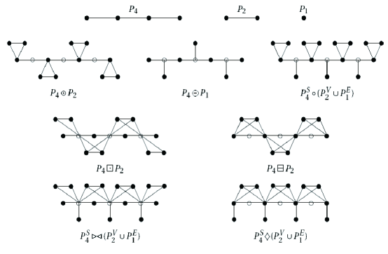
As far as we know, many graph operations such as the disjoint union, the corona, the edge corona and the neighborhood corona have been introduced, and their spectra are computed in [2, 3, 4, 5, 6, 7], respectively. The subdivision graph S(G)𝑆𝐺S(G) of a graph G𝐺G is the graph obtained by inserting a new vertex into every edge of G𝐺G. Based on subdivision graph, the graph operations of subdivision-vertex join and subdivision-edge join are introduced in [8], and their A𝐴A-spectrum are investigated. Further works on their L𝐿L-spectrum are given in [9]. In [11], the spectra of the so called subdivision-vertex corona and subdivision-edge corona are computed, respectively. In [10], the spectra of the subdivision-vertex and subdivision-edge neighborhood corona are computed, respectively. Subsequently, Song and Huang [12] obtained the A𝐴A-spectra and L𝐿L-spectra of the subdivision vertex-edge corona G1S(G2VG3E)superscriptsubscript𝐺1𝑆superscriptsubscript𝐺2𝑉superscriptsubscript𝐺3𝐸G_{1}^{S}\circ(G_{2}^{V}\cup G_{3}^{E}), see P4S(P2VP1E)superscriptsubscript𝑃4𝑆superscriptsubscript𝑃2𝑉superscriptsubscript𝑃1𝐸P_{4}^{S}\circ(P_{2}^{V}\cup P_{1}^{E}) for instance, which is shown in Fig.1.

Motivated by the above works, we define two new graph operations based on subdivision graph as follows. For a graph G1subscript𝐺1G_{1}, let S(G1)𝑆subscript𝐺1S(G_{1}) be the subdividing graph of G1subscript𝐺1G_{1} whose vertex set has two parts: one the original vertices V(G1)𝑉subscript𝐺1V(G_{1}), another, denoted by I(G1)𝐼subscript𝐺1I(G_{1}), the inserting vertices corresponding to the edges of G1subscript𝐺1G_{1}. Let G2subscript𝐺2G_{2} and G3subscript𝐺3G_{3} be other two disjoint graphs.

Definition 1.1.

Subdivision vertex-edge neighbourhood vertex-corona (short for SVEV-corona) of G1subscript𝐺1G_{1} with G2subscript𝐺2G_{2} and G3subscript𝐺3G_{3}, denoted by G1S(G2VG3E)superscriptsubscript𝐺1𝑆superscriptsubscript𝐺2𝑉superscriptsubscript𝐺3𝐸G_{1}^{S}\bowtie(G_{2}^{V}\cup G_{3}^{E}), is the graph consisting of S(G1)𝑆subscript𝐺1S(G_{1}), |V(G1)|𝑉subscript𝐺1|V(G_{1})| copies of G2subscript𝐺2G_{2} and |I(G1)|𝐼subscript𝐺1|I(G_{1})| copies of G3subscript𝐺3G_{3}, all vertex-disjoint, and joining the neighbours of the i-th vertex of V(G1)𝑉subscript𝐺1V(G_{1}) to every vertex in the i-th copy of G2subscript𝐺2G_{2} and i-th vertex of I(G1)𝐼subscript𝐺1I(G_{1}) to each vertex in the i-th copy of G3subscript𝐺3G_{3}.

For instance, we depict P4S(P2VP1E)superscriptsubscript𝑃4𝑆superscriptsubscript𝑃2𝑉superscriptsubscript𝑃1𝐸P_{4}^{S}\bowtie(P_{2}^{V}\cup P_{1}^{E}) in Fig.1. By the definition, G1S(G2VG3E)superscriptsubscript𝐺1𝑆superscriptsubscript𝐺2𝑉superscriptsubscript𝐺3𝐸G_{1}^{S}\bowtie(G_{2}^{V}\cup G_{3}^{E}) has n=n1+m1+n1n2+m1n3𝑛subscript𝑛1subscript𝑚1subscript𝑛1subscript𝑛2subscript𝑚1subscript𝑛3n=n_{1}+m_{1}+n_{1}n_{2}+m_{1}n_{3} vertices and m=2m1+n1m2+m1m3+2m1n2+m1n3𝑚2subscript𝑚1subscript𝑛1subscript𝑚2subscript𝑚1subscript𝑚32subscript𝑚1subscript𝑛2subscript𝑚1subscript𝑛3m=2m_{1}+n_{1}m_{2}+m_{1}m_{3}+2m_{1}n_{2}+m_{1}n_{3} edges, where nisubscript𝑛𝑖n_{i} and misubscript𝑚𝑖m_{i} are the number of vertices and edges of Gisubscript𝐺𝑖G_{i} for i=1,2,3𝑖123i=1,2,3. We see that G1S(G2VG3E)superscriptsubscript𝐺1𝑆superscriptsubscript𝐺2𝑉superscriptsubscript𝐺3𝐸G_{1}^{S}\bowtie(G_{2}^{V}\cup G_{3}^{E}) will be a subdivision-vertex neighbourhood corona (see [10]) if G3subscript𝐺3G_{3} is null, and will be a subdivision-edge corona (see [11]) if G2subscript𝐺2G_{2} is null. Thus subdivision vertex-edge neighbourhood vertex-corona can be viewed as the generalizations of both subdivision-vertex neighbourhood corona (denoted by G1G2subscript𝐺1subscript𝐺2G_{1}\boxdot G_{2}) and subdivision-edge corona (denoted by G1G3subscript𝐺1subscript𝐺3G_{1}\circleddash G_{3}).

Definition 1.2.

Subdivision vertex-edge neighbourhood edge-corona (short for SVEE-corona) of G1subscript𝐺1G_{1} with G2subscript𝐺2G_{2} and G3subscript𝐺3G_{3}, denoted by G1S(G2VG3E)superscriptsubscript𝐺1𝑆superscriptsubscript𝐺2𝑉superscriptsubscript𝐺3𝐸G_{1}^{S}\diamondsuit(G_{2}^{V}\cup G_{3}^{E}), is the graph consisting of S(G1)𝑆subscript𝐺1S(G_{1}), |V(G1)|𝑉subscript𝐺1|V(G_{1})| copies of G2subscript𝐺2G_{2} and |I(G1)|𝐼subscript𝐺1|I(G_{1})| copies of G3subscript𝐺3G_{3}, all vertex-disjoint, joining the neighbours of the i-th vertex of I(G1)𝐼subscript𝐺1I(G_{1}) to every vertex in the i-th copy of G2subscript𝐺2G_{2} and i-th vertex of V(G1)𝑉subscript𝐺1V(G_{1}) to each vertex in the i-th copy of G3subscript𝐺3G_{3}.

For instance, we depict P4S(P2VP1E)superscriptsubscript𝑃4𝑆superscriptsubscript𝑃2𝑉superscriptsubscript𝑃1𝐸P_{4}^{S}\diamondsuit(P_{2}^{V}\cup P_{1}^{E}) in Fig.1. By the definition, G1S(G2VG3E)superscriptsubscript𝐺1𝑆superscriptsubscript𝐺2𝑉superscriptsubscript𝐺3𝐸G_{1}^{S}\diamondsuit(G_{2}^{V}\cup G_{3}^{E}) has n=n1+m1+m1n2+n1n3𝑛subscript𝑛1subscript𝑚1subscript𝑚1subscript𝑛2subscript𝑛1subscript𝑛3n=n_{1}+m_{1}+m_{1}n_{2}+n_{1}n_{3} vertices and m=2m1+m1m2+n1m3+n1n3+2m1n2𝑚2subscript𝑚1subscript𝑚1subscript𝑚2subscript𝑛1subscript𝑚3subscript𝑛1subscript𝑛32subscript𝑚1subscript𝑛2m=2m_{1}+m_{1}m_{2}+n_{1}m_{3}+n_{1}n_{3}+2m_{1}n_{2} edges, where nisubscript𝑛𝑖n_{i} and misubscript𝑚𝑖m_{i} are the number of vertices and edges of Gisubscript𝐺𝑖G_{i} for i=1,2,3𝑖123i=1,2,3. We see that G1S(G2VG3E)superscriptsubscript𝐺1𝑆superscriptsubscript𝐺2𝑉superscriptsubscript𝐺3𝐸G_{1}^{S}\diamondsuit(G_{2}^{V}\cup G_{3}^{E}) will be a subdivision vertex-edge neighbourhood corona (see [10]) if G3subscript𝐺3G_{3} is null, and will be a subdivision edge corona (see [11]) if G2subscript𝐺2G_{2} is null. Thus subdivision vertex-edge neighbourhood edge-corona can be viewed as the generalizations of both subdivision-edge neighbourhood corona (denoted by G1G2subscript𝐺1subscript𝐺2G_{1}\boxminus G_{2}) and subdivision-vertex corona (denoted by G1G3direct-productsubscript𝐺1subscript𝐺3G_{1}\odot G_{3}).

Refer to caption
Figure 1: some related graphs

The normalized Laplacian matrix of a graph is introduced in Chung[1]. It is a rather new but important tool popularized by Chung in 1990s. The normalized Laplacian eigenvalues of a graph have a good relationship with other graph invariants for general graphs in a way that other eigenvalues of matrices (such as the adjacency eigenvalues) fail to do. Thus, for a given graph, calculating its normalized Laplacian spectrum as well as formulating the normalized Laplacian characteristic polynomial is a fundamental and very meaningful work in spectral graph theory. Recently, several graph operations such as subdivisions[14], R𝑅R-graph[15], their normalized Laplacian spectra were computed. In 2017, Das and Panigrahi in [16] have determined the normalized Laplacian spectra of subdivision-vertex(edge)corona[11] and subdivision-vertex (edge) neighbourhood corona[10].

In this paper, we focus on determining the normalized Laplacian spectra of G1S(G2VG3E)superscriptsubscript𝐺1𝑆superscriptsubscript𝐺2𝑉superscriptsubscript𝐺3𝐸G_{1}^{S}\bowtie(G_{2}^{V}\cup G_{3}^{E}) and G1S(G2VG3E)superscriptsubscript𝐺1𝑆superscriptsubscript𝐺2𝑉superscriptsubscript𝐺3𝐸G_{1}^{S}\diamondsuit(G_{2}^{V}\cup G_{3}^{E}) in terms of the corresponding normalized Laplacian spectra of connected regular graphs G1subscript𝐺1G_{1}, G2subscript𝐺2G_{2} and G3subscript𝐺3G_{3}, which extends the corresponding results of [16]. As applications, these results enable us to construct infinitely many pairs of \mathcal{L}-cospectral graphs. Moreover, we also give the number of the spanning trees, the multiplicative degree-Kirchhoff index and Kemeny’s constant of G1S(G2VG3E)superscriptsubscript𝐺1𝑆superscriptsubscript𝐺2𝑉superscriptsubscript𝐺3𝐸G_{1}^{S}\bowtie(G_{2}^{V}\cup G_{3}^{E}) ( G1S(G2VG3E)superscriptsubscript𝐺1𝑆superscriptsubscript𝐺2𝑉superscriptsubscript𝐺3𝐸G_{1}^{S}\diamondsuit(G_{2}^{V}\cup G_{3}^{E}), respectively).

2 Preliminaries

In this section, we first list some known results for latter use.

Lemma 2.1 (​[2]).

For a graph G𝐺G, let R(G)𝑅𝐺R(G) and (G)𝐺\ell(G) be the incidence matrix of G𝐺G and the line graph of G𝐺G, respectively. Then

R(G)TR(G)=2Im+A((G))𝑅superscript𝐺𝑇𝑅𝐺2subscript𝐼𝑚𝐴𝐺R(G)^{T}R(G)=2I_{m}+A(\ell(G)) (1)

where m𝑚m is the number of edges of G𝐺G.

Note that

R(G)R(G)T=D(G)+A(G)=Q(G).𝑅𝐺𝑅superscript𝐺𝑇𝐷𝐺𝐴𝐺𝑄𝐺R(G)R(G)^{T}=D(G)+A(G)=Q(G). (2)

Since non-zero eigenvalues of R(G)R(G)T𝑅𝐺𝑅superscript𝐺𝑇R(G)R(G)^{T} and R(G)TR(G)𝑅superscript𝐺𝑇𝑅𝐺R(G)^{T}R(G) are the same, from the relations (1) and (2) one can obtain

ΦA((G))(x)=(x+2)mnΦQ(G)(x+2).subscriptΦ𝐴𝐺𝑥superscript𝑥2𝑚𝑛subscriptΦ𝑄𝐺𝑥2\Phi_{A(\ell(G))}(x)=(x+2)^{m-n}\Phi_{Q(G)}(x+2). (3)

In particular, if G𝐺G is r𝑟r–regular graph, then by Lemma 2.1, we immediately have the following corollary.

Corollary 2.2.

Let G𝐺G be an r𝑟r–regular graph of order n𝑛n. Then

ΦA((G))(x)=(x+2)mni=1n(x(r2)νi(G)),ΦA((G))(x)=(x+2)mni=1n(x(2r2)+rλi(G))subscriptΦ𝐴𝐺𝑥absentsuperscript𝑥2𝑚𝑛superscriptsubscriptproduct𝑖1𝑛𝑥𝑟2subscript𝜈𝑖𝐺subscriptΦ𝐴𝐺𝑥absentsuperscript𝑥2𝑚𝑛superscriptsubscriptproduct𝑖1𝑛𝑥2𝑟2𝑟subscript𝜆𝑖𝐺\begin{array}[]{ll}\Phi_{A(\ell(G))}(x)&=(x+2)^{m-n}\cdot\prod\limits_{i=1}^{n}(x-(r-2)-\nu_{i}(G)),\\ \Phi_{A(\ell(G))}(x)&=(x+2)^{m-n}\cdot\prod\limits_{i=1}^{n}(x-(2r-2)+r\lambda_{i}(G))\\ \end{array}

where νi(G)subscript𝜈𝑖𝐺\nu_{i}(G) and λi(G)subscript𝜆𝑖𝐺\lambda_{i}(G) arethe eigenvalues of A(G)𝐴𝐺A(G) and (G)𝐺\mathcal{L}(G), respectively .

For a graph matrix M𝑀M of order n𝑛n, we denote by 1nsubscript1𝑛\textbf{1}_{n} and 0nsubscript0𝑛\textbf{0}_{n} the column vector of size n𝑛n with all the entries equal one and all the entries equal 00, respectively. M𝑀M-coronal ΓM(λ)subscriptΓ𝑀𝜆\Gamma_{M}(\lambda) is defined, in [3, 6], to be the sum of the entries of the matrix (λIM)1superscript𝜆𝐼𝑀1(\lambda I-M)^{-1}, i.e.,

ΓM(λ)=1nT(λIM)11n.subscriptΓ𝑀𝜆subscriptsuperscript1𝑇𝑛superscript𝜆𝐼𝑀1subscript1𝑛missing-subexpressionmissing-subexpression\begin{array}[]{ccc}\Gamma_{M}(\lambda)=\textbf{1}^{T}_{n}(\lambda I-M)^{-1}\textbf{1}_{n}.\end{array} (4)

If M𝑀M has constant row sum t𝑡t, it is easy to verify that

ΓM(λ)=1nT1nλt=nλt.subscriptΓ𝑀𝜆subscriptsuperscript1𝑇𝑛subscript1𝑛𝜆𝑡𝑛𝜆𝑡missing-subexpressionmissing-subexpression\begin{array}[]{ccc}\Gamma_{M}(\lambda)=\displaystyle\frac{\textbf{1}^{T}_{n}\textbf{1}_{n}}{\lambda-t}=\frac{n}{\lambda-t}.\end{array} (5)

It is well known for invertible matrix M1subscript𝑀1M_{1} and M4subscript𝑀4M_{4} that

det(M1M2M3M4)=det(M4)det(M1M2M41M3)=det(M1)det(M4M3M11M2).subscript𝑀1subscript𝑀2subscript𝑀3subscript𝑀4absentsubscript𝑀4subscript𝑀1subscript𝑀2superscriptsubscript𝑀41subscript𝑀3missing-subexpressionabsentsubscript𝑀1subscript𝑀4subscript𝑀3superscriptsubscript𝑀11subscript𝑀2\begin{array}[]{rl}\det\left(\begin{array}[]{rl}M_{1}&M_{2}\\ M_{3}&M_{4}\\ \end{array}\right)&=\det(M_{4})\cdot\det(M_{1}-M_{2}M_{4}^{-1}M_{3})\\ &=\det(M_{1})\cdot\det(M_{4}-M_{3}M_{1}^{-1}M_{2}).\end{array} (6)

where M1M2M41M3subscript𝑀1subscript𝑀2superscriptsubscript𝑀41subscript𝑀3M_{1}-M_{2}M_{4}^{-1}M_{3} and M4M3M11M2subscript𝑀4subscript𝑀3superscriptsubscript𝑀11subscript𝑀2M_{4}-M_{3}M_{1}^{-1}M_{2} are called the Schur complements [13] of M4subscript𝑀4M_{4} and M1subscript𝑀1M_{1}, respectively.

For two matrices A=(aij)𝐴subscript𝑎𝑖𝑗A=(a_{ij}) and B=(bij)𝐵subscript𝑏𝑖𝑗B=(b_{ij}), of same size m×n𝑚𝑛m\times n, the Hadamard product AB=(cij)𝐴𝐵subscript𝑐𝑖𝑗A\bullet B=(c_{ij}) of A𝐴A and B𝐵B is a matrix of the same size m×n𝑚𝑛m\times n with entries given by cij=aij×bijsubscript𝑐𝑖𝑗subscript𝑎𝑖𝑗subscript𝑏𝑖𝑗c_{ij}=a_{ij}\times b_{ij}(entrywise multiplication). The Kronecker product ABtensor-product𝐴𝐵A\otimes B of two matrices A=(aij)m×n𝐴subscriptsubscript𝑎𝑖𝑗𝑚𝑛A=(a_{ij})_{m\times n} and B=(bij)p×q𝐵subscriptsubscript𝑏𝑖𝑗𝑝𝑞B=(b_{ij})_{p\times q} is the mp×nq𝑚𝑝𝑛𝑞mp\times nq matrix obtained from A𝐴A by replacing each element aijsubscript𝑎𝑖𝑗a_{ij} by aijBsubscript𝑎𝑖𝑗𝐵a_{ij}B. This is an associative operation with the property that (AB)T=ATBTsuperscripttensor-product𝐴𝐵𝑇tensor-productsuperscript𝐴𝑇superscript𝐵𝑇(A\otimes B)^{T}=A^{T}\otimes B^{T} and (AB)(CD)=ACBDtensor-product𝐴𝐵tensor-product𝐶𝐷tensor-product𝐴𝐶𝐵𝐷(A\otimes B)(C\otimes D)=AC\otimes BD whenever the products AC𝐴𝐶AC and BD𝐵𝐷BD exist. The latter implies (AB)1=A1B1superscripttensor-product𝐴𝐵1tensor-productsuperscript𝐴1superscript𝐵1(A\otimes B)^{-1}=A^{-1}\otimes B^{-1} for nonsingular matrices A𝐴A and B𝐵B. Moreover, if A𝐴A and B𝐵B are n×n𝑛𝑛n\times n and p×p𝑝𝑝p\times p matrices, then det(AB)=det(A)pdet(B)ntensor-product𝐴𝐵superscript𝐴𝑝superscript𝐵𝑛\det(A\otimes B)=\det(A)^{p}\det(B)^{n}. The reader is referred to [7] for other properties of the Kronecker product not mentioned here.

3 The \mathcal{L}-spectra of SVEV-corona and SVEE-corona

In this section, we mainly determe the normalized Laplacian spectrum of SVEV-corona and SVEE-corona, respectively. For the sake of convenience, we write 𝒢=G1S(G2VG3E)𝒢superscriptsubscript𝐺1𝑆superscriptsubscript𝐺2𝑉superscriptsubscript𝐺3𝐸\mathcal{G}=G_{1}^{S}\bowtie(G_{2}^{V}\cup G_{3}^{E}) and 𝔊=G1S(G2VG3E)𝔊superscriptsubscript𝐺1𝑆superscriptsubscript𝐺2𝑉superscriptsubscript𝐺3𝐸\mathfrak{G}=G_{1}^{S}\diamondsuit(G_{2}^{V}\cup G_{3}^{E}) for short. And we respectively denote the eigenvalues of (G1)subscript𝐺1\mathcal{L}(G_{1}), (G2)subscript𝐺2\mathcal{L}(G_{2}) and (G3)subscript𝐺3\mathcal{L}(G_{3}) by θisubscript𝜃𝑖\theta_{i}, μjsubscript𝜇𝑗\mu_{j} and ηksubscript𝜂𝑘\eta_{k} for i,j,k=1,2,,nformulae-sequence𝑖𝑗𝑘12𝑛i,j,k=1,2,\ldots,n. Those symbols will be persisted in what follows.

Theorem 3.1.

Let Gisubscript𝐺𝑖G_{i} be an risubscript𝑟𝑖r_{i}-regular graph with nisubscript𝑛𝑖n_{i} vertices and misubscript𝑚𝑖m_{i} edges, where i=1,2,3𝑖123i=1,2,3. Then

(𝒢)=(In1aR(G1)On1×n1n2On1×m1n3aR(G1)TIm1R(G1)Tbn2TIm1cn3TOn1n2×n1R(G1)bn2In1((G2)B(G2))On1n2×m1n3Om1n3×n1Im1cn3Om1n3×n1n2Im1((G3)B(G3)))𝒢matrixsubscript𝐼subscript𝑛1𝑎𝑅subscript𝐺1subscript𝑂subscript𝑛1subscript𝑛1subscript𝑛2subscript𝑂subscript𝑛1subscript𝑚1subscript𝑛3𝑎𝑅superscriptsubscript𝐺1𝑇subscript𝐼subscript𝑚1tensor-product𝑅superscriptsubscript𝐺1𝑇superscriptsubscript𝑏subscript𝑛2𝑇tensor-productsubscript𝐼subscript𝑚1superscriptsubscript𝑐subscript𝑛3𝑇subscript𝑂subscript𝑛1subscript𝑛2subscript𝑛1tensor-product𝑅subscript𝐺1subscript𝑏subscript𝑛2tensor-productsubscript𝐼subscript𝑛1subscript𝐺2𝐵subscript𝐺2subscript𝑂subscript𝑛1subscript𝑛2subscript𝑚1subscript𝑛3subscript𝑂subscript𝑚1subscript𝑛3subscript𝑛1tensor-productsubscript𝐼subscript𝑚1subscript𝑐subscript𝑛3subscript𝑂subscript𝑚1subscript𝑛3subscript𝑛1subscript𝑛2tensor-productsubscript𝐼subscript𝑚1subscript𝐺3𝐵subscript𝐺3\mathcal{L}(\mathcal{G})=\left(\begin{matrix}I_{n_{1}}\!\!&\!\!-aR(G_{1})\!\!&\!\!O_{n_{1}\times n_{1}n_{2}}\!\!&\!\!O_{n_{1}\times m_{1}n_{3}}\\ -aR(G_{1})^{T}&I_{m_{1}}&-R(G_{1})^{T}\otimes b_{n_{2}}^{T}&-I_{m_{1}}\otimes c_{n_{3}}^{T}\\ O_{n_{1}n_{2}\times n_{1}}\!\!&\!\!-R(G_{1})\otimes b_{n_{2}}\!&\!I_{n_{1}}\otimes(\mathcal{L}(G_{2})\!\bullet\!B(G_{2}))\!\!\!&\!\!\!O_{n_{1}n_{2}\times m_{1}n_{3}}\\ O_{m_{1}n_{3}\times n_{1}}\!\!&\!\!-I_{m_{1}}\otimes c_{n_{3}}\!\!&\!\!O_{m_{1}n_{3}\times n_{1}n_{2}}\!\!&\!\!I_{m_{1}}\otimes(\mathcal{L}(G_{3})\!\bullet\!B(G_{3}))\end{matrix}\right) (7)

where Jnsubscript𝐽𝑛J_{n} is a all-1 matrix of order n𝑛n, and a=1r1(2n2+n3+2)𝑎1subscript𝑟12subscript𝑛2subscript𝑛32a=\frac{1}{\sqrt{r_{1}(2n_{2}+n_{3}+2)}} is a constant. Moreover, bn2=1(r1+r2)(2n2+n3+2)𝟏n2subscript𝑏subscript𝑛21subscript𝑟1subscript𝑟22subscript𝑛2subscript𝑛32subscript1subscript𝑛2b_{n_{2}}=\frac{1}{\sqrt{(r_{1}+r_{2})(2n_{2}+n_{3}+2)}}\mathbf{1}_{n_{2}}, cn3=1(r3+1)(2n2+n3+2)𝟏n3subscript𝑐subscript𝑛31subscript𝑟312subscript𝑛2subscript𝑛32subscript1subscript𝑛3c_{n_{3}}=\frac{1}{\sqrt{(r_{3}+1)(2n_{2}+n_{3}+2)}}\mathbf{1}_{n_{3}}, B(G2)=r2r1+r2Jn2r21r1+r2In2𝐵subscript𝐺2subscript𝑟2subscript𝑟1subscript𝑟2subscript𝐽subscript𝑛2subscript𝑟21subscript𝑟1subscript𝑟2subscript𝐼subscript𝑛2B(G_{2})=\frac{r_{2}}{r_{1}+r_{2}}J_{n_{2}}-\frac{r_{2}-1}{r_{1}+r_{2}}I_{n_{2}}, B(G3)=r3r3+1Jn3r31r3+1In3𝐵subscript𝐺3subscript𝑟3subscript𝑟31subscript𝐽subscript𝑛3subscript𝑟31subscript𝑟31subscript𝐼subscript𝑛3B(G_{3})=\frac{r_{3}}{r_{3}+1}J_{n_{3}}-\frac{r_{3}-1}{r_{3}+1}I_{n_{3}}.

(𝔊)=(In1aR(G1)R(G1)bn2TIn1cn3TaR(G1)TIm1Om1×m1n2Om1×n1n3R(G1)Tbn2Om1n2×m1Im1((G2)B(G2))Om1n2×n1n3In1cn3On1n3×m1On1n3×m1n2In1((G3)B(G3)))𝔊matrixsubscript𝐼subscript𝑛1𝑎𝑅subscript𝐺1tensor-product𝑅subscript𝐺1superscriptsubscript𝑏subscript𝑛2𝑇tensor-productsubscript𝐼subscript𝑛1superscriptsubscript𝑐subscript𝑛3𝑇𝑎𝑅superscriptsubscript𝐺1𝑇subscript𝐼subscript𝑚1subscript𝑂subscript𝑚1subscript𝑚1subscript𝑛2subscript𝑂subscript𝑚1subscript𝑛1subscript𝑛3tensor-product𝑅superscriptsubscript𝐺1𝑇subscript𝑏subscript𝑛2subscript𝑂subscript𝑚1subscript𝑛2subscript𝑚1tensor-productsubscript𝐼subscript𝑚1subscript𝐺2𝐵subscript𝐺2subscript𝑂subscript𝑚1subscript𝑛2subscript𝑛1subscript𝑛3tensor-productsubscript𝐼subscript𝑛1subscript𝑐subscript𝑛3subscript𝑂subscript𝑛1subscript𝑛3subscript𝑚1subscript𝑂subscript𝑛1subscript𝑛3subscript𝑚1subscript𝑛2tensor-productsubscript𝐼subscript𝑛1subscript𝐺3𝐵subscript𝐺3\mathcal{L}(\mathfrak{G})=\left(\begin{matrix}I_{n_{1}}\!&\!-aR(G_{1})\!&\!-R(G_{1})\otimes b_{n_{2}}^{T}\!&\!-I_{n_{1}}\otimes c_{n_{3}}^{T}\\ -aR(G_{1})^{T}&I_{m_{1}}&O_{m_{1}\times m_{1}n_{2}}&O_{m_{1}\times n_{1}n_{3}}\\ -R(G_{1})^{T}\otimes b_{n_{2}}\!\!&\!\!O_{m_{1}n_{2}\times m_{1}}\!&\!I_{m_{1}}\otimes(\mathcal{L}(G_{2})\!\bullet\!B(G_{2}))\!\!\!&\!\!\!O_{m_{1}n_{2}\times n_{1}n_{3}}\\ -I_{n_{1}}\otimes c_{n_{3}}\!\!&\!\!O_{n_{1}n_{3}\times m_{1}}\!\!&\!\!O_{n_{1}n_{3}\times m_{1}n_{2}}\!\!&\!\!I_{n_{1}}\otimes(\mathcal{L}(G_{3})\!\bullet\!B(G_{3}))\end{matrix}\right) (8)

where bn2=1(r2+2)(r1n2+r1+n3)𝟏n2subscript𝑏subscript𝑛21subscript𝑟22subscript𝑟1subscript𝑛2subscript𝑟1subscript𝑛3subscript1subscript𝑛2b_{n_{2}}=\frac{1}{\sqrt{(r_{2}+2)(r_{1}n_{2}+r_{1}+n_{3})}}\mathbf{1}_{n_{2}}, cn3=1(r3+1)(r1n2+r1+n3)𝟏n3subscript𝑐subscript𝑛31subscript𝑟31subscript𝑟1subscript𝑛2subscript𝑟1subscript𝑛3subscript1subscript𝑛3c_{n_{3}}=\frac{1}{\sqrt{(r_{3}+1)(r_{1}n_{2}+r_{1}+n_{3})}}\mathbf{1}_{n_{3}}, B(G2)=r2r2+2Jn2r21r2+2In2𝐵subscript𝐺2subscript𝑟2subscript𝑟22subscript𝐽subscript𝑛2subscript𝑟21subscript𝑟22subscript𝐼subscript𝑛2B(G_{2})=\frac{r_{2}}{r_{2}+2}J_{n_{2}}-\frac{r_{2}-1}{r_{2}+2}I_{n_{2}}, B(G3)=r3r3+1Jn3r31r3+1In3𝐵subscript𝐺3subscript𝑟3subscript𝑟31subscript𝐽subscript𝑛3subscript𝑟31subscript𝑟31subscript𝐼subscript𝑛3B(G_{3})=\frac{r_{3}}{r_{3}+1}J_{n_{3}}-\frac{r_{3}-1}{r_{3}+1}I_{n_{3}}, and a=12(r1n2+r1+n3)𝑎12subscript𝑟1subscript𝑛2subscript𝑟1subscript𝑛3a=\frac{1}{\sqrt{2(r_{1}n_{2}+r_{1}+n_{3})}} is a constant.

Proof.

The proof of Eq.(8) is similar to the Eq.(7), so it’s only necessary to show the result given in Eq.(7) as follows.

We first label the vertices of 𝒢𝒢\mathcal{G}: V(G1)={v1,v2,,vn1}𝑉subscript𝐺1subscript𝑣1subscript𝑣2subscript𝑣subscript𝑛1V(G_{1})=\{v_{1},v_{2},\ldots,v_{n_{1}}\}, I(G1)={e1,e2,,em1}𝐼subscript𝐺1subscript𝑒1subscript𝑒2subscript𝑒subscript𝑚1I(G_{1})=\{e_{1},e_{2},\ldots,e_{m_{1}}\}, V(G2)={u1,u2,,un2}𝑉subscript𝐺2subscript𝑢1subscript𝑢2subscript𝑢subscript𝑛2V(G_{2})=\{u_{1},u_{2},\ldots,u_{n_{2}}\} and V(G3)={w1,w2,,wn3}𝑉subscript𝐺3subscript𝑤1subscript𝑤2subscript𝑤subscript𝑛3V(G_{3})=\{w_{1},w_{2},\ldots,w_{n_{3}}\}. For i=1,2,,n1𝑖12subscript𝑛1i=1,2,\ldots,n_{1}, let Ui={u1i,u2i,U_{i}=\{u_{1}^{i},u_{2}^{i}, ,un2i}\ldots,u_{n_{2}}^{i}\} denote the vertices of the i𝑖i-th copy of G2subscript𝐺2G_{2} in 𝒢𝒢\mathcal{G}, and Wj={w1j,W_{j}=\{w_{1}^{j}, w2j,,wn3j}(j=1,2,,m1)w_{2}^{j},\ldots,w_{n_{3}}^{j}\}~{}(j=1,2,\ldots,m_{1}) the j𝑗j-th copy of G3subscript𝐺3G_{3} in 𝒢𝒢\mathcal{G}. Then the vertices of 𝒢𝒢\mathcal{G} are partitioned by

V(G1)I(G1)(U1U2Un1)(W1W2Wm1).𝑉subscript𝐺1𝐼subscript𝐺1subscript𝑈1subscript𝑈2subscript𝑈subscript𝑛1subscript𝑊1subscript𝑊2subscript𝑊subscript𝑚1missing-subexpressionmissing-subexpression\begin{array}[]{ccc}V(G_{1})\cup I(G_{1})\cup(U_{1}\cup U_{2}\cup\ldots\cup U_{n_{1}})\cup(W_{1}\cup W_{2}\cup\ldots\cup W_{m_{1}}).\end{array} (9)

By Definition 1.1 we see that

{d𝒢(vi)=dG1(vi)=r1,i=1,2,,n1;d𝒢(ei)=2n2+n3+2,i=1,2,,m1;d𝒢(uji)=dG2(uj)+dG1(vi)=r2+r1,j=1,2,,n2,i=1,2,,n1;d𝒢(wji)=dG3(wj)+1=r3+1,j=1,2,,n3,i=1,2,,m1.casessubscript𝑑𝒢subscript𝑣𝑖formulae-sequenceabsentsubscript𝑑subscript𝐺1subscript𝑣𝑖subscript𝑟1𝑖12subscript𝑛1subscript𝑑𝒢subscript𝑒𝑖formulae-sequenceabsent2subscript𝑛2subscript𝑛32𝑖12subscript𝑚1subscript𝑑𝒢superscriptsubscript𝑢𝑗𝑖formulae-sequenceabsentsubscript𝑑subscript𝐺2subscript𝑢𝑗subscript𝑑subscript𝐺1subscript𝑣𝑖subscript𝑟2subscript𝑟1formulae-sequence𝑗12subscript𝑛2𝑖12subscript𝑛1subscript𝑑𝒢superscriptsubscript𝑤𝑗𝑖formulae-sequenceabsentsubscript𝑑subscript𝐺3subscript𝑤𝑗1subscript𝑟31formulae-sequence𝑗12subscript𝑛3𝑖12subscript𝑚1\left\{\begin{array}[]{rl}d_{\mathcal{G}}(v_{i})&=d_{G_{1}}(v_{i})=r_{1},\hskip 142.26378pti=1,2,\ldots,n_{1};\\ d_{\mathcal{G}}(e_{i})&=2n_{2}+n_{3}+2,\hskip 142.26378pti=1,2,\ldots,m_{1};\\ d_{\mathcal{G}}(u_{j}^{i})&=d_{G_{2}}(u_{j})+d_{G_{1}}(v_{i})=r_{2}+r_{1},\hskip 56.9055ptj=1,2,\ldots,n_{2},i=1,2,\ldots,n_{1};\\ d_{\mathcal{G}}(w_{j}^{i})&=d_{G_{3}}(w_{j})+1=r_{3}+1,\hskip 85.35826ptj=1,2,\ldots,n_{3},i=1,2,\ldots,m_{1}.\end{array}\right.

Let R(G1)𝑅subscript𝐺1R(G_{1}) be the vertex-edge incidence matrix of G1subscript𝐺1G_{1}. Then the adjacency matrix of 𝒢𝒢\mathcal{G} can be represented in the form of block-matrix according to the ordering of (9) in the following.

A(𝒢)=(On1×n1R(G1)On1×n1n2On1×m1n3R(G1)TOm1×m1R(G1)T1n2TIm11n3TOn1n2×n1R(G1)1n2In1A(G2)On1n2×m1n3Om1n3×n1Im11n3Om1n3×n1n2Im1A(G3)),𝐴𝒢matrixsubscript𝑂subscript𝑛1subscript𝑛1𝑅subscript𝐺1subscript𝑂subscript𝑛1subscript𝑛1subscript𝑛2subscript𝑂subscript𝑛1subscript𝑚1subscript𝑛3𝑅superscriptsubscript𝐺1𝑇subscript𝑂subscript𝑚1subscript𝑚1tensor-product𝑅superscriptsubscript𝐺1𝑇superscriptsubscript1subscript𝑛2𝑇tensor-productsubscript𝐼subscript𝑚1superscriptsubscript1subscript𝑛3𝑇subscript𝑂subscript𝑛1subscript𝑛2subscript𝑛1tensor-product𝑅subscript𝐺1subscript1subscript𝑛2tensor-productsubscript𝐼subscript𝑛1𝐴subscript𝐺2subscript𝑂subscript𝑛1subscript𝑛2subscript𝑚1subscript𝑛3subscript𝑂subscript𝑚1subscript𝑛3subscript𝑛1tensor-productsubscript𝐼subscript𝑚1subscript1subscript𝑛3subscript𝑂subscript𝑚1subscript𝑛3subscript𝑛1subscript𝑛2tensor-productsubscript𝐼subscript𝑚1𝐴subscript𝐺3A(\mathcal{G})=\left(\begin{matrix}O_{n_{1}\times n_{1}}~{}&R(G_{1})~{}&O_{n_{1}\times n_{1}n_{2}}~{}&O_{n_{1}\times m_{1}n_{3}}\\ R(G_{1})^{T}~{}&O_{m_{1}\times m_{1}}~{}&R(G_{1})^{T}\otimes\textbf{1}_{n_{2}}^{T}~{}&I_{m_{1}}\otimes\textbf{1}_{n_{3}}^{T}\\ O_{n_{1}n_{2}\times n_{1}}~{}&R(G_{1})\otimes\textbf{1}_{n_{2}}~{}&I_{n_{1}}\otimes A(G_{2})~{}&O_{n_{1}n_{2}\times m_{1}n_{3}}\\ O_{m_{1}n_{3}\times n_{1}}~{}&I_{m_{1}}\otimes\textbf{1}_{n_{3}}~{}&O_{m_{1}n_{3}\times n_{1}n_{2}}~{}&I_{m_{1}}\otimes A(G_{3})\end{matrix}\right),

and

D(𝒢)=(r1In1(2n2+n3+2)Im1(r1+r2)In1n2(r3+1)Im1n3)𝐷𝒢matrixsubscript𝑟1subscript𝐼subscript𝑛1missing-subexpressionmissing-subexpressionmissing-subexpressionmissing-subexpression2subscript𝑛2subscript𝑛32subscript𝐼subscript𝑚1missing-subexpressionmissing-subexpressionmissing-subexpressionmissing-subexpressionsubscript𝑟1subscript𝑟2subscript𝐼subscript𝑛1subscript𝑛2missing-subexpressionmissing-subexpressionmissing-subexpressionmissing-subexpressionsubscript𝑟31subscript𝐼subscript𝑚1subscript𝑛3D(\mathcal{G})=\left(\begin{matrix}r_{1}I_{n_{1}}\!\!\!&\!\!\!\!\!\!&\!\!\!\!\!\!&\!\!\!\\ \!\!\!&\!\!\!(2n_{2}+n_{3}+2)I_{m_{1}}\!\!\!&\!\!\!\!\!\!&\!\!\!\\ \!\!&\!\!\!\!&\!\!(r_{1}+r_{2})I_{n_{1}n_{2}}\!\!&\!\!\\ \!\!&\!\!\!\!&\!\!\!\!&\!\!(r_{3}+1)I_{m_{1}n_{3}}\end{matrix}\right)

where A(G2)𝐴subscript𝐺2A(G_{2}) and A(G3)𝐴subscript𝐺3A(G_{3}) represent the adjacency matrices of G2subscript𝐺2G_{2} and G3subscript𝐺3G_{3}, respectively.

Since G2subscript𝐺2G_{2} is an r2subscript𝑟2r_{2}-regular graph, we have (G2)=In21r2A(G2)subscript𝐺2subscript𝐼subscript𝑛21subscript𝑟2𝐴subscript𝐺2\mathcal{L}(G_{2})=I_{n_{2}}-\frac{1}{r_{2}}A(G_{2}). Thus,

(G2)B(G2)=(In21r2A(G2))B(G2)=In21r1+r2A(G2).subscript𝐺2𝐵subscript𝐺2subscript𝐼subscript𝑛21subscript𝑟2𝐴subscript𝐺2𝐵subscript𝐺2subscript𝐼subscript𝑛21subscript𝑟1subscript𝑟2𝐴subscript𝐺2\mathcal{L}(G_{2})\bullet B(G_{2})=(I_{n_{2}}-\frac{1}{r_{2}}A(G_{2}))\bullet B(G_{2})=I_{n_{2}}-\frac{1}{r_{1}+r_{2}}A(G_{2}).

By direct computation, one can obtain that

In1n21r1+r2In1A(G2)=In1((G2)B(G2)).subscript𝐼subscript𝑛1subscript𝑛2tensor-product1subscript𝑟1subscript𝑟2subscript𝐼subscript𝑛1𝐴subscript𝐺2tensor-productsubscript𝐼subscript𝑛1subscript𝐺2𝐵subscript𝐺2I_{n_{1}n_{2}}-\frac{1}{r_{1}+r_{2}}I_{n_{1}}\otimes A(G_{2})=I_{n_{1}}\otimes(\mathcal{L}(G_{2})\bullet B(G_{2})).

Furthermore, we can obtain that

Im1n31r3+1Im1A(G3)=Im1((G3)B(G3)).subscript𝐼subscript𝑚1subscript𝑛3tensor-product1subscript𝑟31subscript𝐼subscript𝑚1𝐴subscript𝐺3tensor-productsubscript𝐼subscript𝑚1subscript𝐺3𝐵subscript𝐺3I_{m_{1}n_{3}}-\frac{1}{r_{3}+1}I_{m_{1}}\otimes A(G_{3})=I_{m_{1}}\otimes(\mathcal{L}(G_{3})\bullet B(G_{3})).

By (𝒢)=ID(𝒢)1/2A(𝒢)D(𝒢)1/2𝒢𝐼𝐷superscript𝒢12𝐴𝒢𝐷superscript𝒢12\mathcal{L}(\mathcal{G})=I-D(\mathcal{G})^{-1/2}A(\mathcal{G})D(\mathcal{G})^{-1/2}, the required normalized Laplacian matrix is given below:

(𝒢)=(In1aR(G1)On1×n1n2On1×m1n3aR(G1)TIm1R(G1)Tbn2TIm1cn3TOn1n2×n1R(G1)bn2In1((G2)B(G2))On1n2×m1n3Om1n3×n1Im1cn3Om1n3×n1n2Im1((G3)B(G3))).𝒢matrixsubscript𝐼subscript𝑛1𝑎𝑅subscript𝐺1subscript𝑂subscript𝑛1subscript𝑛1subscript𝑛2subscript𝑂subscript𝑛1subscript𝑚1subscript𝑛3𝑎𝑅superscriptsubscript𝐺1𝑇subscript𝐼subscript𝑚1tensor-product𝑅superscriptsubscript𝐺1𝑇superscriptsubscript𝑏subscript𝑛2𝑇tensor-productsubscript𝐼subscript𝑚1superscriptsubscript𝑐subscript𝑛3𝑇subscript𝑂subscript𝑛1subscript𝑛2subscript𝑛1tensor-product𝑅subscript𝐺1subscript𝑏subscript𝑛2tensor-productsubscript𝐼subscript𝑛1subscript𝐺2𝐵subscript𝐺2subscript𝑂subscript𝑛1subscript𝑛2subscript𝑚1subscript𝑛3subscript𝑂subscript𝑚1subscript𝑛3subscript𝑛1tensor-productsubscript𝐼subscript𝑚1subscript𝑐subscript𝑛3subscript𝑂subscript𝑚1subscript𝑛3subscript𝑛1subscript𝑛2tensor-productsubscript𝐼subscript𝑚1subscript𝐺3𝐵subscript𝐺3\mathcal{L}(\mathcal{G})=\left(\begin{matrix}I_{n_{1}}\!&\!-aR(G_{1})\!&\!O_{n_{1}\times n_{1}n_{2}}\!&\!O_{n_{1}\times m_{1}n_{3}}\\ -aR(G_{1})^{T}&I_{m_{1}}&-R(G_{1})^{T}\otimes b_{n_{2}}^{T}&-I_{m_{1}}\otimes c_{n_{3}}^{T}\\ O_{n_{1}n_{2}\times n_{1}}\!\!&\!\!-R(G_{1})\otimes b_{n_{2}}\!&\!I_{n_{1}}\otimes(\mathcal{L}(G_{2})\!\bullet\!B(G_{2}))\!\!\!&\!\!\!O_{n_{1}n_{2}\times m_{1}n_{3}}\\ O_{m_{1}n_{3}\times n_{1}}\!\!&\!\!-I_{m_{1}}\otimes c_{n_{3}}\!\!&\!\!O_{m_{1}n_{3}\times n_{1}n_{2}}\!\!&\!\!I_{m_{1}}\otimes(\mathcal{L}(G_{3})\!\bullet\!B(G_{3}))\end{matrix}\right).

The proof is completed. ∎

Remark 1.

Obviously, using the same partition of (9) to the graph 𝔊𝔊\mathfrak{G}, one can obtain

{d𝔊(ei)=2,i=1,2,,m1;d𝔊(uji)=dG2(uj)+2=r2+2,j=1,2,,n2,i=1,2,,n1;d𝔊(wji)=dG3(wj)+1=r3+1,j=1,2,,n3,i=1,2,,m1;d𝔊(vi)=(n2+1)dG1(vi)+n3=(n2+1)r1+n3,i=1,2,,n1;casessubscript𝑑𝔊subscript𝑒𝑖formulae-sequenceabsent2𝑖12subscript𝑚1subscript𝑑𝔊superscriptsubscript𝑢𝑗𝑖formulae-sequenceabsentsubscript𝑑subscript𝐺2subscript𝑢𝑗2subscript𝑟22formulae-sequence𝑗12subscript𝑛2𝑖12subscript𝑛1subscript𝑑𝔊superscriptsubscript𝑤𝑗𝑖formulae-sequenceabsentsubscript𝑑subscript𝐺3subscript𝑤𝑗1subscript𝑟31formulae-sequence𝑗12subscript𝑛3𝑖12subscript𝑚1subscript𝑑𝔊subscript𝑣𝑖formulae-sequenceabsentsubscript𝑛21subscript𝑑subscript𝐺1subscript𝑣𝑖subscript𝑛3subscript𝑛21subscript𝑟1subscript𝑛3𝑖12subscript𝑛1\left\{\begin{array}[]{rl}d_{\mathfrak{G}}(e_{i})&=2,\ \hskip 184.9429pti=1,2,\ldots,m_{1};\\ d_{\mathfrak{G}}(u_{j}^{i})&=d_{G_{2}}(u_{j})+2=r_{2}+2,\hskip 99.58464ptj=1,2,\ldots,n_{2},i=1,2,\ldots,n_{1};\\ d_{\mathfrak{G}}(w_{j}^{i})&=d_{G_{3}}(w_{j})+1=r_{3}+1,\hskip 99.58464ptj=1,2,\ldots,n_{3},i=1,2,\ldots,m_{1};\\ d_{\mathfrak{G}}(v_{i})&=(n_{2}+1)d_{G_{1}}(v_{i})+n_{3}=(n_{2}+1)r_{1}+n_{3},\hskip 17.07182pti=1,2,\ldots,n_{1};\\ \end{array}\right.

and

A(𝔊)=(On1×n1R(G1)R(G1)1n2TIn11n3TRT(G1)Om1×m1Im10n2TRT(G1)0n3TRT(G1)1n2Im10n2Im1A(G2)RT(G1)On2×n3TIn11n3R(G1)0n3R(G1)On3×n2In1A(G3)).𝐴𝔊matrixsubscript𝑂subscript𝑛1subscript𝑛1𝑅subscript𝐺1tensor-product𝑅subscript𝐺1superscriptsubscript1subscript𝑛2𝑇tensor-productsubscript𝐼subscript𝑛1subscriptsuperscript1𝑇subscript𝑛3superscript𝑅𝑇subscript𝐺1subscript𝑂subscript𝑚1subscript𝑚1tensor-productsubscript𝐼subscript𝑚1superscriptsubscript0subscript𝑛2𝑇tensor-productsuperscript𝑅𝑇subscript𝐺1subscriptsuperscript0𝑇subscript𝑛3tensor-productsuperscript𝑅𝑇subscript𝐺1subscript1subscript𝑛2tensor-productsubscript𝐼subscript𝑚1subscript0subscript𝑛2tensor-productsubscript𝐼subscript𝑚1𝐴subscript𝐺2tensor-productsuperscript𝑅𝑇subscript𝐺1superscriptsubscript𝑂subscript𝑛2subscript𝑛3𝑇tensor-productsubscript𝐼subscript𝑛1subscript1subscript𝑛3tensor-product𝑅subscript𝐺1subscript0subscript𝑛3tensor-product𝑅subscript𝐺1subscript𝑂subscript𝑛3subscript𝑛2tensor-productsubscript𝐼subscript𝑛1𝐴subscript𝐺3A(\mathfrak{G})=\left(\begin{matrix}O_{n_{1}\times n_{1}}~{}&R(G_{1})~{}&R(G_{1})\otimes~{}\textbf{1}_{n_{2}}^{T}~{}&I_{n_{1}}~{}\otimes~{}\textbf{1}^{T}_{n_{3}}\\ R^{T}(G_{1})~{}&O_{m_{1}\times m_{1}}~{}&I_{m_{1}}\otimes~{}\textbf{0}_{n_{2}}^{T}~{}&R^{T}(G_{1})\otimes~{}\textbf{0}^{T}_{n_{3}}\\ R^{T}(G_{1})\otimes~{}\textbf{1}_{n_{2}}~{}&I_{m_{1}}~{}\otimes~{}\textbf{0}_{n_{2}}~{}&I_{m_{1}}\otimes~{}A(G_{2})~{}&R^{T}(G_{1})~{}\otimes~{}O_{n_{2}\times n_{3}}^{T}\\ I_{n_{1}}\otimes~{}\textbf{1}_{n_{3}}~{}&R(G_{1})\otimes~{}\textbf{0}_{n_{3}}~{}&R(G_{1})\otimes~{}O_{n_{3}\times n_{2}}~{}&I_{n_{1}}\otimes~{}A(G_{3})\end{matrix}\right).

By immediate calculation, the (𝔊)𝔊\mathcal{L}(\mathfrak{G}) follows.

Theorem 3.2.

Let Gisubscript𝐺𝑖G_{i} be an risubscript𝑟𝑖r_{i}-regular graph with nisubscript𝑛𝑖n_{i} vertices and misubscript𝑚𝑖m_{i} edges, where i=1,2,3𝑖123i=1,2,3. Then

(i)Φ(𝒢)(λ)=(λ1n3(r3+1)(2n2+n3+2)(λ1r3+1))m1n1j=1n2(λr1+r2μjr1+r2)n1k=1n3(λ1+r3ηkr3+1)m1×i=1n1((λ1)(λ1n3(r3+1)(2n2+n3+2)(λ1r3+1))(2θi)((r1+r2+n2r1)λ(1+n2)r1)(r1+r2)(2n2+n3+2)(λr1r1+r2));\begin{array}[]{rl}\emph{(i)}\hskip 5.69046pt\Phi_{\mathcal{L}(\mathcal{G})}(\lambda)\!\!\!\!&=\!\displaystyle(\lambda\!\!-\!\!1\!\!-\!\frac{n_{3}}{(r_{3}\!\!+\!\!1)(2n_{2}\!\!+\!\!n_{3}\!\!+\!\!2)(\lambda\!\!-\!\!\frac{1}{r_{3}+1})})^{m_{1}\!-\!n_{1}}\!\!\cdot\!\!\textstyle\prod\limits_{j=1}^{n_{2}}(\lambda\!\!-\!\frac{r_{1}+r_{2}\mu_{j}}{r_{1}+r_{2}})^{n_{1}}\!\!\cdot\!\!\prod\limits_{k=1}^{n_{3}}(\lambda\!\!-\!\frac{1+r_{3}\eta_{k}}{r_{3}+1})^{m_{1}}\\ &\times\!\textstyle\prod\limits_{i=1}^{n_{1}}\big{(}(\lambda\!-\!1)(\lambda\!-\!1\!-\!\frac{n_{3}}{(r_{3}+1)(2n_{2}+n_{3}+2)(\lambda-\frac{1}{r_{3}+1})})\!-\!\frac{(2-\theta_{i})((r_{1}+r_{2}+n_{2}r_{1})\lambda-(1+n_{2})r_{1})}{(r_{1}+r_{2})(2n_{2}+n_{3}+2)(\lambda-\frac{r_{1}}{r_{1}+r_{2}})}\big{)};\end{array}
(ii)Φ(𝔊)(λ)=(λ1)m1n1j=1n2(λ2+r2μjr2+2)m1k=1n3(λ1+r3ηkr3+1)n1×i=1n1((λ1)(λ1n3(r3+1)(r1n2+n3+r1)(λ1r3+1))r1(2θi)((2n2+r2+2)λ2n22)2(r2+2)(r1n2+n3+r1)(λ2r2+2))\begin{array}[]{rl}\emph{(ii)}\hskip 5.69046pt\Phi_{\mathcal{L}(\mathfrak{G})}(\lambda)\!\!\!\!&=\!\displaystyle(\lambda\!-\!1)^{m_{1}\!-\!n_{1}}\!\cdot\!\textstyle\prod\limits_{j=1}^{n_{2}}(\lambda\!\!-\!\frac{2+r_{2}\mu_{j}}{r_{2}+2})^{m_{1}}\!\cdot\!\prod\limits_{k=1}^{n_{3}}(\lambda\!\!-\!\frac{1+r_{3}\eta_{k}}{r_{3}+1})^{n_{1}}\\ &\times\!\textstyle\prod\limits_{i=1}^{n_{1}}\big{(}(\lambda\!-\!1)(\lambda\!-\!1\!-\!\frac{n_{3}}{(r_{3}+1)(r_{1}n_{2}+n_{3}+r_{1})(\lambda-\frac{1}{r_{3}+1})})\!-\!\frac{r_{1}(2-\theta_{i})((2n_{2}+r_{2}+2)\lambda-2n_{2}-2)}{2(r_{2}+2)(r_{1}n_{2}+n_{3}+r_{1})(\lambda-\frac{2}{r_{2}+2})}\big{)}\end{array}

where θisubscript𝜃𝑖\theta_{i}, μjsubscript𝜇𝑗\mu_{j} and ηksubscript𝜂𝑘\eta_{k} are the eigenvalues of (G1)subscript𝐺1\mathcal{L}(G_{1}), (G2)subscript𝐺2\mathcal{L}(G_{2}) and (G3)subscript𝐺3\mathcal{L}(G_{3}), respectively.

Proof.

According to Theorem 3.1, the normalized Laplacian characteristic polynomial of 𝒢𝒢\mathcal{G} is

Φ(𝒢)(λ)=det(λIn(𝒢))=det(B0),subscriptΦ𝒢𝜆𝜆subscript𝐼𝑛𝒢subscript𝐵0\Phi_{\mathcal{L}(\mathcal{G})}(\lambda)=\det(\lambda I_{n}-\mathcal{L}(\mathcal{G}))=\det(B_{0}),

where

B0=((λ1)In1aR(G1)OOaR(G1)T(λ1)Im1R(G1)Tbn2TIm1cn3TOR(G1)bn2In1(λIn2(G2)B(G2))OOIm1cn3OIm1(λIn3(G3)B(G3))).subscript𝐵0𝜆1subscript𝐼subscript𝑛1𝑎𝑅subscript𝐺1𝑂𝑂𝑎𝑅superscriptsubscript𝐺1𝑇𝜆1subscript𝐼subscript𝑚1tensor-product𝑅superscriptsubscript𝐺1𝑇superscriptsubscript𝑏subscript𝑛2𝑇tensor-productsubscript𝐼subscript𝑚1superscriptsubscript𝑐subscript𝑛3𝑇𝑂tensor-product𝑅subscript𝐺1subscript𝑏subscript𝑛2tensor-productsubscript𝐼subscript𝑛1𝜆subscript𝐼subscript𝑛2subscript𝐺2𝐵subscript𝐺2𝑂𝑂tensor-productsubscript𝐼subscript𝑚1subscript𝑐subscript𝑛3𝑂tensor-productsubscript𝐼subscript𝑚1𝜆subscript𝐼subscript𝑛3subscript𝐺3𝐵subscript𝐺3B_{0}=\left(\begin{smallmatrix}(\lambda-1)I_{n_{1}}~{}~{}~{}~{}&~{}~{}~{}~{}aR(G_{1})~{}~{}~{}~{}&~{}~{}~{}~{}O~{}~{}~{}~{}&~{}~{}~{}~{}O\\ aR(G_{1})^{T}&(\lambda-1)I_{m_{1}}&R(G_{1})^{T}\otimes b_{n_{2}}^{T}&I_{m_{1}}\otimes c_{n_{3}}^{T}\\ O&R(G_{1})\otimes b_{n_{2}}&I_{n_{1}}\otimes(\lambda I_{n_{2}}-\mathcal{L}(G_{2})\bullet B(G_{2}))&O\\ O&I_{m_{1}}\otimes c_{n_{3}}&O&I_{m_{1}}\otimes(\lambda I_{n_{3}}-\mathcal{L}(G_{3})\bullet B(G_{3}))\end{smallmatrix}\right).

We write P𝑃P as the elementary block matrix below

P=(In1OOOOIm1R(G1)T(bn2T(λIn2(G2)B(G2))1)Im1(cn3T(λIn3(G3)B(G3))1)OOIn1In2OOOOIm1In3).𝑃subscript𝐼subscript𝑛1𝑂𝑂𝑂𝑂subscript𝐼subscript𝑚1tensor-product𝑅superscriptsubscript𝐺1𝑇superscriptsubscript𝑏subscript𝑛2𝑇superscript𝜆subscript𝐼subscript𝑛2subscript𝐺2𝐵subscript𝐺21tensor-productsubscript𝐼subscript𝑚1superscriptsubscript𝑐subscript𝑛3𝑇superscript𝜆subscript𝐼subscript𝑛3subscript𝐺3𝐵subscript𝐺31𝑂𝑂tensor-productsubscript𝐼subscript𝑛1subscript𝐼subscript𝑛2𝑂𝑂𝑂𝑂tensor-productsubscript𝐼subscript𝑚1subscript𝐼subscript𝑛3P=\left(\begin{smallmatrix}I_{n_{1}}\!&\!O\!&\!O\!&\!O\\ O&I_{m_{1}}~{}&-R(G_{1})^{T}\otimes(b_{n_{2}}^{T}(\lambda I_{n_{2}}-\mathcal{L}(G_{2})\bullet B(G_{2}))^{-1})~{}&-I_{m_{1}}\otimes(c_{n_{3}}^{T}(\lambda I_{n_{3}}-\mathcal{L}(G_{3})\bullet B(G_{3}))^{-1})\\ O&O&I_{n_{1}}\otimes I_{n_{2}}&O\\ O&O&O&I_{m_{1}}\otimes I_{n_{3}}\end{smallmatrix}\right).

Let B=PB0𝐵𝑃subscript𝐵0B=PB_{0}. Then

B=((λ1)In1aR(G1)OOaR(G1)T(λ1Γ3(λ))Im1Γ2(λ)R(G1)TR(G1)OOOR(G1)bn2In1(λIn2(G2)B(G2))OOIm1cn3OIm1(λIn3(G3)B(G3)))𝐵𝜆1subscript𝐼subscript𝑛1𝑎𝑅subscript𝐺1𝑂𝑂𝑎𝑅superscriptsubscript𝐺1𝑇𝜆1subscriptΓ3𝜆subscript𝐼subscript𝑚1subscriptΓ2𝜆𝑅superscriptsubscript𝐺1𝑇𝑅subscript𝐺1𝑂𝑂𝑂tensor-product𝑅subscript𝐺1subscript𝑏subscript𝑛2tensor-productsubscript𝐼subscript𝑛1𝜆subscript𝐼subscript𝑛2subscript𝐺2𝐵subscript𝐺2𝑂𝑂tensor-productsubscript𝐼subscript𝑚1subscript𝑐subscript𝑛3𝑂tensor-productsubscript𝐼subscript𝑚1𝜆subscript𝐼subscript𝑛3subscript𝐺3𝐵subscript𝐺3B=\left(\begin{smallmatrix}(\lambda-1)I_{n_{1}}\!\!&\!\!aR(G_{1})\!\!&\!\!O\!\!&\!\!O\\ aR(G_{1})^{T}&(\lambda-1-\Gamma_{3}(\lambda))I_{m_{1}}\!-\Gamma_{2}(\lambda)R(G_{1})^{T}R(G_{1})&O&O\\ O\!&\!R(G_{1})\otimes b_{n_{2}}\!\!&\!\!I_{n_{1}}\otimes(\lambda I_{n_{2}}\!-\mathcal{L}(G_{2})\bullet B(G_{2}))\!&\!O\\ O\!&\!I_{m_{1}}\otimes c_{n_{3}}\!&\!O\!\!&\!\!I_{m_{1}}\otimes(\lambda I_{n_{3}}\!-\mathcal{L}(G_{3})\bullet B(G_{3}))\end{smallmatrix}\right)

where Γ2(λ)=bn2T(λIn2(G2)B(G2))1bn2subscriptΓ2𝜆superscriptsubscript𝑏subscript𝑛2𝑇superscript𝜆subscript𝐼subscript𝑛2subscript𝐺2𝐵subscript𝐺21subscript𝑏subscript𝑛2\Gamma_{2}(\lambda)=b_{n_{2}}^{T}(\lambda I_{n_{2}}-\mathcal{L}(G_{2})\bullet B(G_{2}))^{-1}b_{n_{2}} and Γ3(λ)=cn3T(λIn3(G3)B(G3))1cn3subscriptΓ3𝜆superscriptsubscript𝑐subscript𝑛3𝑇superscript𝜆subscript𝐼subscript𝑛3subscript𝐺3𝐵subscript𝐺31subscript𝑐subscript𝑛3\Gamma_{3}(\lambda)=c_{n_{3}}^{T}(\lambda I_{n_{3}}-\mathcal{L}(G_{3})\bullet B(G_{3}))^{-1}c_{n_{3}}.

Note that det(P)=1𝑃1\det(P)=1. Then we have

Φ(𝒢)(λ)=det(B0)=det(P1)det(B)=det(B).subscriptΦ𝒢𝜆subscript𝐵0superscript𝑃1𝐵𝐵\Phi_{\mathcal{L}(\mathcal{G})}(\lambda)=\det(B_{0})=\det(P^{-1})\det(B)=\det(B).

For the matrix B𝐵B, one can get

det(B)=det(In1(λIn2(G2)B(G2)))det(Im1(λIn3(G3)B(G3)))det(S1),𝐵tensor-productsubscript𝐼subscript𝑛1𝜆subscript𝐼subscript𝑛2subscript𝐺2𝐵subscript𝐺2tensor-productsubscript𝐼subscript𝑚1𝜆subscript𝐼subscript𝑛3subscript𝐺3𝐵subscript𝐺3subscript𝑆1\det(B)\!\!=\!\!\det\big{(}I_{n_{1}}\!\!\otimes(\lambda I_{n_{2}}\!\!-\!\mathcal{L}(G_{2})\bullet B(G_{2}))\big{)}\cdot\det\big{(}I_{m_{1}}\!\!\otimes(\lambda I_{n_{3}}\!\!-\!\mathcal{L}(G_{3})\bullet B(G_{3}))\big{)}\cdot\det(S_{1}),

where

S1=((λ1)In1aR(G1)aR(G1)T(λ1Γ3(λ))Im1Γ2(λ)R(G1)TR(G1)).subscript𝑆1matrix𝜆1subscript𝐼subscript𝑛1𝑎𝑅subscript𝐺1𝑎𝑅superscriptsubscript𝐺1𝑇𝜆1subscriptΓ3𝜆subscript𝐼subscript𝑚1subscriptΓ2𝜆𝑅superscriptsubscript𝐺1𝑇𝑅subscript𝐺1S_{1}=\left(\begin{matrix}(\lambda-1)I_{n_{1}}&aR(G_{1})\\ aR(G_{1})^{T}&(\lambda-1-\Gamma_{3}(\lambda))I_{m_{1}}\!-\Gamma_{2}(\lambda)R(G_{1})^{T}R(G_{1})\end{matrix}\right).

Let θisubscript𝜃𝑖\theta_{i}, μjsubscript𝜇𝑗\mu_{j} and ηksubscript𝜂𝑘\eta_{k} be the eigenvalues of (G1)subscript𝐺1\mathcal{L}(G_{1}), (G2)subscript𝐺2\mathcal{L}(G_{2}) and (G3)subscript𝐺3\mathcal{L}(G_{3}), respectively. By applying Eq.(6), the following result follows from Corollary 2.2 that

det(S1)=|(λ1)In1aR(G1)aR(G1)T(λ1Γ3(λ))Im1Γ2(λ)R(G1)TR(G1)|=det((λ1)In1)det((λ1Γ3(λ))Im1(Γ2(λ)+a2λ1)R(G1)TR(G1)).=(λ1)n1det((λ1Γ3(λ))Im1(Γ2(λ)+a2λ1)(A((G1))+2Im1))=(λ1)n1((λ1Γ3(λ))(Γ2(λ)+a2λ1)(2+2))m1n1×det((λ1Γ3(λ))In1(Γ2(λ)+a2λ1)(2r1In1r1(G1))=(λ1Γ3(λ))m1n1det((λ1)(λ1Γ3(λ))In1r1((λ1)Γ2(λ)+a2)(2In1(G1)))=(λ1Γ3(λ))m1n1i=1n1((λ1)(λ1Γ3(λ))r1((λ1)Γ2(λ)+1r1(2n2+n3+2))(2θi)).\begin{array}[]{rl}\det(S_{1})&=\left|\begin{array}[]{cc}(\lambda-1)I_{n_{1}}&aR(G_{1})\\ \vspace{0.2cm}aR(G_{1})^{T}&(\lambda-1-\Gamma_{3}(\lambda))I_{m_{1}}\!-\Gamma_{2}(\lambda)R(G_{1})^{T}R(G_{1})\end{array}\right|\\ &=\displaystyle\det((\lambda-1)I_{n_{1}})\cdot\det((\lambda-1-\Gamma_{3}(\lambda))I_{m_{1}}-(\Gamma_{2}(\lambda)+\frac{a^{2}}{\lambda-1})R(G_{1})^{T}R(G_{1})).\\ &=\displaystyle(\lambda-1)^{n_{1}}\det\big{(}(\lambda-1-\Gamma_{3}(\lambda))I_{m_{1}}-(\Gamma_{2}(\lambda)+\frac{a^{2}}{\lambda-1})(A(\ell(G_{1}))+2I_{m_{1}})\big{)}\\ &=\displaystyle(\lambda-1)^{n_{1}}\cdot\big{(}(\lambda-1-\Gamma_{3}(\lambda))-(\Gamma_{2}(\lambda)+\frac{a^{2}}{\lambda-1})(-2+2)\big{)}^{m_{1}-n_{1}}\\ \vspace{0.2cm}\hfil&\hskip 14.22636pt\times\displaystyle~{}\det\big{(}(\lambda-1-\Gamma_{3}(\lambda))I_{n_{1}}-(\Gamma_{2}(\lambda)+\frac{a^{2}}{\lambda-1})(2r_{1}I_{n_{1}}-r_{1}\mathcal{L}(G_{1})\big{)}\\ &=\displaystyle(\lambda\!\!-\!1\!\!-\!\!\Gamma_{3}(\lambda))^{m_{1}\!-\!n_{1}}\!\cdot\!\det\big{(}(\lambda\!-\!1)(\lambda\!\!-\!1\!\!-\!\!\Gamma_{3}(\lambda))I_{n_{1}}\!\!\!-\!r_{1}((\lambda\!-\!1)\Gamma_{2}(\lambda)\!+\!a^{2})(2I_{n_{1}}\!\!\!-\!\!\mathcal{L}(G_{1}))\big{)}\\ &=\displaystyle(\lambda\!\!-\!1\!\!-\!\!\Gamma_{3}(\lambda))^{m_{1}\!-\!n_{1}}\!\cdot\!\textstyle\prod\limits_{i=1}^{n_{1}}\big{(}(\lambda\!-\!1)(\lambda\!\!-\!1\!\!-\!\!\Gamma_{3}(\lambda))\!-\!r_{1}((\lambda\!-\!1)\Gamma_{2}(\lambda)\!+\!\frac{1}{r_{1}(2n_{2}+n_{3}+2)})(2\!-\!\theta_{i})\big{)}.\end{array}

Since (G2)B(G2)=In21r1+r2A(G2)subscript𝐺2𝐵subscript𝐺2subscript𝐼subscript𝑛21subscript𝑟1subscript𝑟2𝐴subscript𝐺2\mathcal{L}(G_{2})\bullet B(G_{2})=I_{n_{2}}-\frac{1}{r_{1}+r_{2}}A(G_{2}) and A(G2)=r2(In2(G2))𝐴subscript𝐺2subscript𝑟2subscript𝐼subscript𝑛2subscript𝐺2A(G_{2})=r_{2}(I_{n_{2}}-\mathcal{L}(G_{2})), we get

(G2)B(G2)=1r1+r2(r1In2+r2(G2)).subscript𝐺2𝐵subscript𝐺21subscript𝑟1subscript𝑟2subscript𝑟1subscript𝐼subscript𝑛2subscript𝑟2subscript𝐺2\mathcal{L}(G_{2})\bullet B(G_{2})=\frac{1}{r_{1}+r_{2}}(r_{1}I_{n_{2}}+r_{2}\mathcal{L}(G_{2})).

Similarly, (G3)B(G3)=1r3+1(In3+r3(G3))subscript𝐺3𝐵subscript𝐺31subscript𝑟31subscript𝐼subscript𝑛3subscript𝑟3subscript𝐺3\mathcal{L}(G_{3})\bullet B(G_{3})=\frac{1}{r_{3}+1}(I_{n_{3}}+r_{3}\mathcal{L}(G_{3})).

Also since G2subscript𝐺2G_{2} is r2subscript𝑟2r_{2}-regular, the sum of all entries on every row of its normalized Laplacian matrix is zero. In other words, (G2)bn2=(1r2r2)bn2=0bn2=0subscript𝐺2subscript𝑏subscript𝑛21subscript𝑟2subscript𝑟2subscript𝑏subscript𝑛20subscript𝑏subscript𝑛20\mathcal{L}(G_{2})b_{n_{2}}=(1-\frac{r_{2}}{r_{2}})b_{n_{2}}=0\cdot b_{n_{2}}=\textbf{0}. Then ((G2)B(G2))bn2=(1r2r1+r2)bn2=r1r1+r2bn2subscript𝐺2𝐵subscript𝐺2subscript𝑏subscript𝑛21subscript𝑟2subscript𝑟1subscript𝑟2subscript𝑏subscript𝑛2subscript𝑟1subscript𝑟1subscript𝑟2subscript𝑏subscript𝑛2(\mathcal{L}(G_{2})\bullet B(G_{2}))b_{n_{2}}=(1-\frac{r_{2}}{r_{1}+r_{2}})b_{n_{2}}=\frac{r_{1}}{r_{1}+r_{2}}b_{n_{2}} and (λIn2((G2)B(G2)))bn2=(λr1r1+r2)bn2𝜆subscript𝐼subscript𝑛2subscript𝐺2𝐵subscript𝐺2subscript𝑏subscript𝑛2𝜆subscript𝑟1subscript𝑟1subscript𝑟2subscript𝑏subscript𝑛2(\lambda I_{n_{2}}-(\mathcal{L}(G_{2})\bullet B(G_{2})))b_{n_{2}}=(\lambda-\frac{r_{1}}{r_{1}+r_{2}})b_{n_{2}}. Also, bn2Tbn2=n2(r1+r2)(2n2+n3+2)superscriptsubscript𝑏subscript𝑛2𝑇subscript𝑏subscript𝑛2subscript𝑛2subscript𝑟1subscript𝑟22subscript𝑛2subscript𝑛32b_{n_{2}}^{T}b_{n_{2}}=\frac{n_{2}}{(r_{1}+r_{2})(2n_{2}+n_{3}+2)}. Thus

Γ2(λ)=bn2T(λIn2(G2)B(G2))1bn2=bn2Tbn2λr1r1+r2=n2(r1+r2)(2n2+n3+2)(λr1r1+r2).subscriptΓ2𝜆superscriptsubscript𝑏subscript𝑛2𝑇superscript𝜆subscript𝐼subscript𝑛2subscript𝐺2𝐵subscript𝐺21subscript𝑏subscript𝑛2superscriptsubscript𝑏subscript𝑛2𝑇subscript𝑏subscript𝑛2𝜆subscript𝑟1subscript𝑟1subscript𝑟2subscript𝑛2subscript𝑟1subscript𝑟22subscript𝑛2subscript𝑛32𝜆subscript𝑟1subscript𝑟1subscript𝑟2\Gamma_{2}(\lambda)=b_{n_{2}}^{T}(\lambda I_{n_{2}}-\mathcal{L}(G_{2})\bullet B(G_{2}))^{-1}b_{n_{2}}=\frac{b_{n_{2}}^{T}b_{n_{2}}}{\lambda-\frac{r_{1}}{r_{1}+r_{2}}}=\frac{n_{2}}{(r_{1}+r_{2})(2n_{2}+n_{3}+2)(\lambda-\frac{r_{1}}{r_{1}+r_{2}})}.

The value of Γ3(λ)subscriptΓ3𝜆\Gamma_{3}(\lambda) is similar to that of Γ2(λ)subscriptΓ2𝜆\Gamma_{2}(\lambda), and so,

Γ3(λ)=cn3T(λIn3(G3)B(G3))1cn3=cn3Tcn3λ1r3+1=n3(r3+1)(2n2+n3+2)(λ1r3+1).subscriptΓ3𝜆superscriptsubscript𝑐subscript𝑛3𝑇superscript𝜆subscript𝐼subscript𝑛3subscript𝐺3𝐵subscript𝐺31subscript𝑐subscript𝑛3superscriptsubscript𝑐subscript𝑛3𝑇subscript𝑐subscript𝑛3𝜆1subscript𝑟31subscript𝑛3subscript𝑟312subscript𝑛2subscript𝑛32𝜆1subscript𝑟31\Gamma_{3}(\lambda)=c_{n_{3}}^{T}(\lambda I_{n_{3}}-\mathcal{L}(G_{3})\bullet B(G_{3}))^{-1}c_{n_{3}}=\frac{c_{n_{3}}^{T}c_{n_{3}}}{\lambda-\frac{1}{r_{3}+1}}=\frac{n_{3}}{(r_{3}+1)(2n_{2}+n_{3}+2)(\lambda-\frac{1}{r_{3}+1})}.

In summary, the normalized Laplacian characteristic polynomial of 𝒢𝒢\mathcal{G} is

Φ(𝒢)(λ)=j=1n2(λr1+r2μjr1+r2)n1k=1n3(λ1+r3ηkr3+1)m1det(S1)=(λ1n3(r3+1)(2n2+n3+2)(λ1r3+1))m1n1j=1n2(λr1+r2μjr1+r2)n1k=1n3(λ1+r3ηkr3+1)m1×i=1n1((λ1)(λ1n3(r3+1)(2n2+n3+2)(λ1r3+1))(2θi)((r1+r2+n2r1)λ(1+n2)r1)(r1+r2)(2n2+n3+2)(λr1r1+r2)),\begin{array}[]{rl}\Phi_{\mathcal{L}(\mathcal{G})}(\lambda)\!\!\!\!&=\displaystyle\textstyle\prod\limits_{j=1}^{n_{2}}(\lambda-\frac{r_{1}+r_{2}\mu_{j}}{r_{1}+r_{2}})^{n_{1}}\cdot\prod\limits_{k=1}^{n_{3}}(\lambda-\frac{1+r_{3}\eta_{k}}{r_{3}+1})^{m_{1}}\cdot\det(S_{1})\\ &=\!\displaystyle(\lambda\!\!-\!\!1\!\!-\!\frac{n_{3}}{(r_{3}\!\!+\!\!1)(2n_{2}\!\!+\!\!n_{3}\!\!+\!\!2)(\lambda\!\!-\!\!\frac{1}{r_{3}+1})})^{m_{1}\!-\!n_{1}}\!\!\cdot\!\!\textstyle\prod\limits_{j=1}^{n_{2}}(\lambda\!\!-\!\frac{r_{1}+r_{2}\mu_{j}}{r_{1}+r_{2}})^{n_{1}}\!\!\cdot\!\!\prod\limits_{k=1}^{n_{3}}(\lambda\!\!-\!\frac{1+r_{3}\eta_{k}}{r_{3}+1})^{m_{1}}\\ &\times\!\textstyle\prod\limits_{i=1}^{n_{1}}\big{(}(\lambda\!-\!1)(\lambda\!-\!1\!-\!\frac{n_{3}}{(r_{3}+1)(2n_{2}+n_{3}+2)(\lambda-\frac{1}{r_{3}+1})})\!-\!\frac{(2-\theta_{i})((r_{1}+r_{2}+n_{2}r_{1})\lambda-(1+n_{2})r_{1})}{(r_{1}+r_{2})(2n_{2}+n_{3}+2)(\lambda-\frac{r_{1}}{r_{1}+r_{2}})}\big{)},\end{array}

as required. The proof of (ii) is similar to the (i). ∎

Remark 2.

In Theorem 3.2, if one of graphs G2subscript𝐺2G_{2} and G3subscript𝐺3G_{3} is null in 𝒢𝒢\mathcal{G} or 𝔊𝔊\mathfrak{G}, then one can directly deduce the main results(see Theorems 2.2-2.5) due to A. Das and P. Panigrahi in [16]. For the simplicity, we here omit Theorems 2.2-2.5 belonged to A. Das and P. Panigrahi[16].

From Threom 3.2, one can easily obtain the following corollaries.

Corollary 3.3.

Let Gisubscript𝐺𝑖G_{i} be an risubscript𝑟𝑖r_{i}-regular graph with nisubscript𝑛𝑖n_{i} vertices and misubscript𝑚𝑖m_{i} edges for i=1,2,3𝑖123i=1,2,3. Then the normalized Laplacian spectrum of 𝒢𝒢\mathcal{G} consist of:

  1. (a)

    r1+r2μjr1+r2subscript𝑟1subscript𝑟2subscript𝜇𝑗subscript𝑟1subscript𝑟2\frac{r_{1}+r_{2}\mu_{j}}{r_{1}+r_{2}} repeated n1subscript𝑛1n_{1} times for each eigenvalue μjsubscript𝜇𝑗\mu_{j} of (G2)subscript𝐺2\mathcal{L}(G_{2}), j=1,2,,n21𝑗12subscript𝑛21j=1,2,\ldots,n_{2}-1;

  2. (b)

    1+r3ηkr3+11subscript𝑟3subscript𝜂𝑘subscript𝑟31\frac{1+r_{3}\eta_{k}}{r_{3}+1} repeated m1subscript𝑚1m_{1} times for each eigenvalue ηksubscript𝜂𝑘\eta_{k} of (G3)subscript𝐺3\mathcal{L}(G_{3}), k=1,2,,n31𝑘12subscript𝑛31k=1,2,\ldots,n_{3}-1;

  3. (c)

    two roots of the equation

    (2n2r3+n3r3+2r3+2n2+n3+2)λ2(2n2r3+n3r3+2r3+4n2+2n3+4)λ+2n2+2=0\begin{array}[]{rl}&(2n_{2}r_{3}+n_{3}r_{3}+2r_{3}+2n_{2}+n_{3}+2)\lambda^{2}-(2n_{2}r_{3}+n_{3}r_{3}+2r_{3}+4n_{2}\\ &+2n_{3}+4)\lambda+2n_{2}+2=0\end{array} (10)

    where each root repeats m1n1subscript𝑚1subscript𝑛1m_{1}-n_{1} times;

  4. (d)

    four roots of the equation

    (2n2+n3+2)((1+r3)λ1)((r1+r2)λr1)(λ1)2n3(λ1)((r1+r2)λr1)(2θi)((r1+r2+n2r1)λ(r1+r1n2))((1+r3)λ1)=0,\begin{array}[]{rl}&(2n_{2}+n_{3}+2)((1+r_{3})\lambda-1)((r_{1}+r_{2})\lambda-r_{1})(\lambda-1)^{2}-n_{3}(\lambda-1)((r_{1}+r_{2})\lambda\\ &-r_{1})-(2-\theta_{i})\big{(}(r_{1}+r_{2}+n_{2}r_{1})\lambda-(r_{1}+r_{1}n_{2})\big{)}((1+r_{3})\lambda-1)=0,\end{array} (11)

    where each eigenvalue θisubscript𝜃𝑖\theta_{i} of (G1)subscript𝐺1\mathcal{L}(G_{1}), i=1,2,,n1𝑖12subscript𝑛1i=1,2,\ldots,n_{1}.

Corollary 3.4.

If Gisubscript𝐺𝑖G_{i} is an risubscript𝑟𝑖r_{i}-regular graph with nisubscript𝑛𝑖n_{i} vertices and misubscript𝑚𝑖m_{i} edges for i=1,2,3𝑖123i=1,2,3, the normalized Laplacian spectrum of 𝔊𝔊\mathfrak{G} consist of:

  1. (a)

    2+r2μjr2+22subscript𝑟2subscript𝜇𝑗subscript𝑟22\frac{2+r_{2}\mu_{j}}{r_{2}+2} repeated m1subscript𝑚1m_{1} times for each eigenvalue μjsubscript𝜇𝑗\mu_{j} of (G2)subscript𝐺2\mathcal{L}(G_{2}), j=1,2,,n21𝑗12subscript𝑛21j=1,2,\ldots,n_{2}-1;

  2. (b)

    1+r3ηkr3+11subscript𝑟3subscript𝜂𝑘subscript𝑟31\frac{1+r_{3}\eta_{k}}{r_{3}+1} repeated n1subscript𝑛1n_{1} times for each eigenvalue ηksubscript𝜂𝑘\eta_{k} of (G3)subscript𝐺3\mathcal{L}(G_{3}), k=1,2,,n31𝑘12subscript𝑛31k=1,2,\ldots,n_{3}-1;

  3. (c)

    111 repeats m1n1subscript𝑚1subscript𝑛1m_{1}-n_{1} times, 2r2+22subscript𝑟22\frac{2}{r_{2}+2} repeats m1n1subscript𝑚1subscript𝑛1m_{1}-n_{1} times;

  4. (d)

    four roots of the equation

    2(r1n2+n3+r1)((1+r3)λ1)((2+r2)λ2)(λ1)22n3(λ1)((2+r2)λ2)r1(2θi)((2n2+r2+2)λ2n22)((1+r3)λ1)=0,missing-subexpression2subscript𝑟1subscript𝑛2subscript𝑛3subscript𝑟11subscript𝑟3𝜆12subscript𝑟2𝜆2superscript𝜆122subscript𝑛3𝜆12subscript𝑟2𝜆2missing-subexpressionsubscript𝑟12subscript𝜃𝑖2subscript𝑛2subscript𝑟22𝜆2subscript𝑛221subscript𝑟3𝜆10\begin{array}[]{rl}&2(r_{1}n_{2}+n_{3}+r_{1})((1+r_{3})\lambda-1)((2+r_{2})\lambda-2)(\lambda-1)^{2}-2n_{3}(\lambda-1)((2+r_{2})\lambda-2)\\ &-r_{1}(2-\theta_{i})\big{(}(2n_{2}+r_{2}+2)\lambda-2n_{2}-2\big{)}((1+r_{3})\lambda-1)=0,\end{array}

    where each eigenvalue θisubscript𝜃𝑖\theta_{i} of (G1)subscript𝐺1\mathcal{L}(G_{1}), i=1,2,,n1𝑖12subscript𝑛1i=1,2,\ldots,n_{1}.

Example 1.

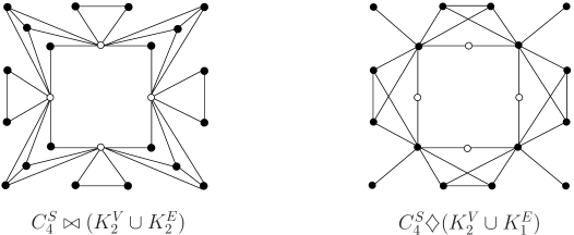
Let G=C4S(K2VK2E)𝐺superscriptsubscript𝐶4𝑆superscriptsubscript𝐾2𝑉superscriptsubscript𝐾2𝐸G=C_{4}^{S}\bowtie(K_{2}^{V}\cup K_{2}^{E}) and H=C4S(K2VK1E)𝐻superscriptsubscript𝐶4𝑆superscriptsubscript𝐾2𝑉superscriptsubscript𝐾1𝐸H=C_{4}^{S}\diamondsuit(K_{2}^{V}\cup K_{1}^{E}) (shown in Fig.2). By simple computation, Spec(C4)={0,1,1,2}𝑆𝑝𝑒subscript𝑐subscript𝐶40112Spec_{\mathcal{L}}(C_{4})=\{0,1,1,2\}, Spec(K2)={0,2}𝑆𝑝𝑒subscript𝑐subscript𝐾202Spec_{\mathcal{L}}(K_{2})=\{0,2\} and Spec(K1)={0}𝑆𝑝𝑒subscript𝑐subscript𝐾10Spec_{\mathcal{L}}(K_{1})=\{0\}.

From Corollary 3.3, the normalized Laplacian spectrum of G𝐺G consist of: 4343\frac{4}{3} (multiplicity 4), 3232\frac{3}{2} (multiplicity 4), four roots of the equation 24x476x3+71x220x=024superscript𝑥476superscript𝑥371superscript𝑥220𝑥024x^{4}-76x^{3}+71x^{2}-20x=0, four roots (multiplicity 2) of the equation 48x4152x3+156x259x+6=048superscript𝑥4152superscript𝑥3156superscript𝑥259𝑥6048x^{4}-152x^{3}+156x^{2}-59x+6=0, and four roots of the equation 48x4152x3+170x278x+12=048superscript𝑥4152superscript𝑥3170superscript𝑥278𝑥12048x^{4}-152x^{3}+170x^{2}-78x+12=0.

From Corollary 3.4, the normalized Laplacian spectrum of H𝐻H consist of: 4343\frac{4}{3} (multiplicity 4), four roots of the equation 42x4154x3+176x264x=042superscript𝑥4154superscript𝑥3176superscript𝑥264𝑥042x^{4}-154x^{3}+176x^{2}-64x=0, four roots (multiplicity 2) of the equation 42x4154x3+190x290x+12=042superscript𝑥4154superscript𝑥3190superscript𝑥290𝑥12042x^{4}-154x^{3}+190x^{2}-90x+12=0, and four roots of the equation 42x4154x3+204x2116x+24=042superscript𝑥4154superscript𝑥3204superscript𝑥2116𝑥24042x^{4}-154x^{3}+204x^{2}-116x+24=0.

Refer to caption
Figure 2: G=C4S(K2VK2E)𝐺superscriptsubscript𝐶4𝑆superscriptsubscript𝐾2𝑉superscriptsubscript𝐾2𝐸G=C_{4}^{S}\bowtie(K_{2}^{V}\cup K_{2}^{E}) and H=C4S(K2VK1E)𝐻superscriptsubscript𝐶4𝑆superscriptsubscript𝐾2𝑉superscriptsubscript𝐾1𝐸H=C_{4}^{S}\diamondsuit(K_{2}^{V}\cup K_{1}^{E})

4 Applications

In this section, we will give four distinct applications, such as construction for \mathcal{L}-cospectral graphs, computation for the number of spanning trees, the multiplicative degree-Kirchhoff index and Kemeny’s constant on SVEV-corona and SVEE-corona respectively.

4.1 Construct \mathcal{L}-cospectral graphs

In [17], Dam and Haemers have proposed ‘Which graphs are determined by their spectra?’. The question for the normalized Laplacian spectrum is also one of the outstanding unsolved problems in the theory of graph spectra. Thus, if one wish to settle the question for graphs in general, it is natural to look for constructing pairs of \mathcal{L}-cospectral graphs. In this section, we will respectively construct many infinite families of pairs of \mathcal{L}-cospectral graphs from SVEV-corona and SVEE-corona, which are generalized Theorem 2.7 due to Das and Panigrahi in [16].

Theorem 4.1.

Let Gisubscript𝐺𝑖G_{i} and Hisubscript𝐻𝑖H_{i} (not necessarily distinct isomorphic) are pairwise \mathcal{L}-cospectral regular graphs for i=1,2,3𝑖123i=1,2,3. Then

  1. (1)

    G1S(G2VG3E)superscriptsubscript𝐺1𝑆superscriptsubscript𝐺2𝑉superscriptsubscript𝐺3𝐸G_{1}^{S}\bowtie(G_{2}^{V}\cup G_{3}^{E}) and H1S(H2VH3E)superscriptsubscript𝐻1𝑆superscriptsubscript𝐻2𝑉superscriptsubscript𝐻3𝐸H_{1}^{S}\bowtie(H_{2}^{V}\cup H_{3}^{E}) are \mathcal{L}-cospectral graphs;

  2. (2)

    G1S(G2VG3E)superscriptsubscript𝐺1𝑆superscriptsubscript𝐺2𝑉superscriptsubscript𝐺3𝐸G_{1}^{S}\diamondsuit(G_{2}^{V}\cup G_{3}^{E}) and H1S(H2VH3E)superscriptsubscript𝐻1𝑆superscriptsubscript𝐻2𝑉superscriptsubscript𝐻3𝐸H_{1}^{S}\diamondsuit(H_{2}^{V}\cup H_{3}^{E}) are \mathcal{L}-cospectral graphs.

Proof.

From Theorem 3.2 we know that, the normalized Laplacian spectra of G1S(G2VG3E)superscriptsubscript𝐺1𝑆superscriptsubscript𝐺2𝑉superscriptsubscript𝐺3𝐸G_{1}^{S}\bowtie(G_{2}^{V}\cup G_{3}^{E}) and G1Ssuperscriptsubscript𝐺1𝑆G_{1}^{S}\diamondsuit (G2VG3E)superscriptsubscript𝐺2𝑉superscriptsubscript𝐺3𝐸(G_{2}^{V}\cup G_{3}^{E}) are completely determined by the degrees of regularities, the number of vertices, the number of edges and the normalized Laplacian spectra of regular graphs Gisubscript𝐺𝑖G_{i} (i=1,2,3)𝑖123(i=1,2,3). So the conclusions follows. ∎

Remark 3.

Let G1subscript𝐺1G_{1} and H1subscript𝐻1H_{1} be two \mathcal{L}-cospectral graphs. If {Gi(1),Gi(2),Gi(3),}superscriptsubscript𝐺𝑖1superscriptsubscript𝐺𝑖2superscriptsubscript𝐺𝑖3\{G_{i}^{(1)},G_{i}^{(2)},G_{i}^{(3)},\ldots\} and {Hi(1),Hi(2),\{H_{i}^{(1)},H_{i}^{(2)}, Hi(3),}H_{i}^{(3)},\ldots\} are two pairwise \mathcal{L}-cospectral but not isomorphic graph sequences for i=2,3𝑖23i=2,3. We wonder what conditions such that the largest infinite families of pairs of (G1S(G2(1)VG3(1)E))(G2(2)VG3(2)E)superscriptsubscript𝐺1𝑆superscriptsubscript𝐺21𝑉superscriptsubscript𝐺31𝐸superscriptsubscript𝐺22𝑉superscriptsubscript𝐺32𝐸(G_{1}^{S}\bowtie(G_{2}^{(1)V}\cup G_{3}^{(1)E}))\bowtie(G_{2}^{(2)V}\cup G_{3}^{(2)E})\cdots and (H1S(H2(1)VH3(1)E))(H2(2)VH3(2)E)superscriptsubscript𝐻1𝑆superscriptsubscript𝐻21𝑉superscriptsubscript𝐻31𝐸superscriptsubscript𝐻22𝑉superscriptsubscript𝐻32𝐸(H_{1}^{S}\bowtie(H_{2}^{(1)V}\cup H_{3}^{(1)E}))\bowtie(H_{2}^{(2)V}\cup H_{3}^{(2)E})\cdots, and (G1S(G2(1)VG3(1)E))(G2(2)VG3(2)E)superscriptsubscript𝐺1𝑆superscriptsubscript𝐺21𝑉superscriptsubscript𝐺31𝐸superscriptsubscript𝐺22𝑉superscriptsubscript𝐺32𝐸(G_{1}^{S}\diamondsuit(G_{2}^{(1)V}\cup G_{3}^{(1)E}))\diamondsuit(G_{2}^{(2)V}\cup G_{3}^{(2)E})\cdots and (H1S(H2(1)VH3(1)E))superscriptsubscript𝐻1𝑆superscriptsubscript𝐻21𝑉superscriptsubscript𝐻31𝐸(H_{1}^{S}\diamondsuit(H_{2}^{(1)V}\cup H_{3}^{(1)E})) (H2(2)VH3(2)E)superscriptsubscript𝐻22𝑉superscriptsubscript𝐻32𝐸\diamondsuit(H_{2}^{(2)V}\cup H_{3}^{(2)E})\cdots are \mathcal{L}-cospectral ?

Example 2.

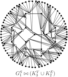
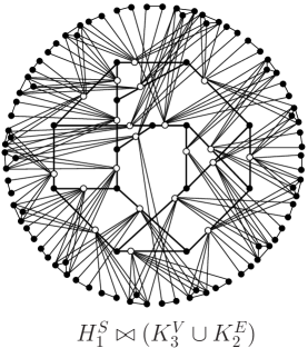
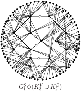
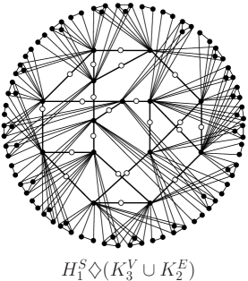
Let G1subscript𝐺1G_{1} and H1subscript𝐻1H_{1} be two graphs shown in Fig.3. Then by Matlab 7.0 one can get ΦA(G1)(x)=ΦA(H1)(x)=x1421x122x11+164x10+22x9599x888x7+1047x6+168x5800x4160x3+216x2+40x12subscriptΦ𝐴subscript𝐺1𝑥subscriptΦ𝐴subscript𝐻1𝑥superscript𝑥1421superscript𝑥122superscript𝑥11164superscript𝑥1022superscript𝑥9599superscript𝑥888superscript𝑥71047superscript𝑥6168superscript𝑥5800superscript𝑥4160superscript𝑥3216superscript𝑥240𝑥12\Phi_{A(G_{1})}(x)=\Phi_{A(H_{1})}(x)=x^{14}-21x^{12}-2x^{11}+164x^{10}+22x^{9}-599x^{8}-88x^{7}+1047x^{6}+168x^{5}-800x^{4}-160x^{3}+216x^{2}+40x-12. It is easy to see that G1subscript𝐺1G_{1} and H1subscript𝐻1H_{1} are A𝐴A-cospectral but not isomorphic with each other. Note that =ID1/2AD1/2𝐼superscript𝐷12𝐴superscript𝐷12\mathcal{L}=I-D^{-1/2}AD^{-1/2}. And so, two graphs are A𝐴A-cospectral imply that they are \mathcal{L}-cospectral. Consequently, it follows from Theorem 4.1 that G1S(K3VK2E)superscriptsubscript𝐺1𝑆superscriptsubscript𝐾3𝑉superscriptsubscript𝐾2𝐸G_{1}^{S}\bowtie(K_{3}^{V}\cup K_{2}^{E}) and H1S(K3VK2E)superscriptsubscript𝐻1𝑆superscriptsubscript𝐾3𝑉superscriptsubscript𝐾2𝐸H_{1}^{S}\bowtie(K_{3}^{V}\cup K_{2}^{E}) are \mathcal{L}-cospectral graphs, so are G1S(K3VK2E)superscriptsubscript𝐺1𝑆superscriptsubscript𝐾3𝑉superscriptsubscript𝐾2𝐸G_{1}^{S}\diamondsuit(K_{3}^{V}\cup K_{2}^{E}) and H1S(K3VK2E)superscriptsubscript𝐻1𝑆superscriptsubscript𝐾3𝑉superscriptsubscript𝐾2𝐸H_{1}^{S}\diamondsuit(K_{3}^{V}\cup K_{2}^{E}), see Fig.4 and Fig.5 for instance.
Refer to caption
Figure 3: G1subscript𝐺1G_{1} and H1subscript𝐻1H_{1}
Refer to caption
Refer to caption
Figure 4: G1S(K3VK2E)superscriptsubscript𝐺1𝑆superscriptsubscript𝐾3𝑉superscriptsubscript𝐾2𝐸G_{1}^{S}\bowtie(K_{3}^{V}\cup K_{2}^{E}) and H1S(K3VK2E)superscriptsubscript𝐻1𝑆superscriptsubscript𝐾3𝑉superscriptsubscript𝐾2𝐸H_{1}^{S}\bowtie(K_{3}^{V}\cup K_{2}^{E})
Refer to caption
Refer to caption
Figure 5: G1S(K3VK2E)superscriptsubscript𝐺1𝑆superscriptsubscript𝐾3𝑉superscriptsubscript𝐾2𝐸G_{1}^{S}\diamondsuit(K_{3}^{V}\cup K_{2}^{E}) and H1S(K3VK2E)superscriptsubscript𝐻1𝑆superscriptsubscript𝐾3𝑉superscriptsubscript𝐾2𝐸H_{1}^{S}\diamondsuit(K_{3}^{V}\cup K_{2}^{E})

4.2 The number of spanning trees

Let G𝐺G be a connected graph of order n𝑛n. A spanning tree is a spanning subgraph of G𝐺G that is a tree. A known result from Chung [1] allows the calculation of this number from the normalized Laplacian spectrum and the degrees of all the vertices, thus the number of spanning trees τ(G)𝜏𝐺\tau(G) of connected graph G𝐺G is

τ(G)=Πi=1ndiΠi=1n1λii=1ndi.𝜏𝐺superscriptsubscriptΠ𝑖1𝑛subscript𝑑𝑖superscriptsubscriptΠ𝑖1𝑛1subscript𝜆𝑖superscriptsubscript𝑖1𝑛subscript𝑑𝑖\hskip 136.5733pt\tau(G)=\displaystyle\frac{\Pi_{i=1}^{n}d_{i}\Pi_{i=1}^{n-1}\lambda_{i}}{\sum_{i=1}^{n}d_{i}}. (12)
Theorem 4.2.

Let Gisubscript𝐺𝑖G_{i} be an risubscript𝑟𝑖r_{i}-regular graph with nisubscript𝑛𝑖n_{i} vertices and misubscript𝑚𝑖m_{i} edges for i=1,2,3𝑖123i=1,2,3. Then

(1)τ(𝒢)=i=1n11θij=1n21(r1+r2μj)n1k=1n31(1+r3ηk)m1r12n11(1+n2)m11×2m1n11n3r1r3+4n2r1+2n2r2+2n3r1+4r12m1+n1m2+m1m3+2m1n2+m1n3.1𝜏𝒢absentsuperscriptsubscriptproduct𝑖1subscript𝑛11subscript𝜃𝑖superscriptsubscriptproduct𝑗1subscript𝑛21superscriptsubscript𝑟1subscript𝑟2subscript𝜇𝑗subscript𝑛1superscriptsubscriptproduct𝑘1subscript𝑛31superscript1subscript𝑟3subscript𝜂𝑘subscript𝑚1superscriptsubscript𝑟12subscript𝑛11superscript1subscript𝑛2subscript𝑚11missing-subexpressionabsentsuperscript2subscript𝑚1subscript𝑛11subscript𝑛3subscript𝑟1subscript𝑟34subscript𝑛2subscript𝑟12subscript𝑛2subscript𝑟22subscript𝑛3subscript𝑟14subscript𝑟12subscript𝑚1subscript𝑛1subscript𝑚2subscript𝑚1subscript𝑚32subscript𝑚1subscript𝑛2subscript𝑚1subscript𝑛3\begin{array}[]{rl}(1)~{}~{}\tau(\mathcal{G})&=\prod\limits_{i=1}^{n_{1}-1}\!\theta_{i}\cdot\!\prod\limits_{j=1}^{n_{2}-1}\!(r_{1}\!+\!r_{2}\mu_{j})^{n_{1}}\!\cdot\!\prod\limits_{k=1}^{n_{3}-1}\!(1\!+\!r_{3}\eta_{k})^{m_{1}}\!\cdot\!r_{1}^{2n_{1}-1}\cdot(1+n_{2})^{m_{1}-1}\\ \vspace{0.2cm}\hfil&\displaystyle\times 2^{m_{1}-n_{1}-1}\cdot\frac{n_{3}r_{1}r_{3}+4n_{2}r_{1}+2n_{2}r_{2}+2n_{3}r_{1}+4r_{1}}{2m_{1}+n_{1}m_{2}+m_{1}m_{3}+2m_{1}n_{2}+m_{1}n_{3}}.\\ \end{array}
(2)τ(𝔊)=22m1n11i=1n11(r1+r1n2)θij=1n21(2+r2μj)m1k=1n31(1+r3ηk)n1×n2r1r2+4n2r1+2n3r3+4n3+4r12m1+m1m2+n1m3+n1n3+2m1n2.2𝜏𝔊absentsuperscript22subscript𝑚1subscript𝑛11superscriptsubscriptproduct𝑖1subscript𝑛11subscript𝑟1subscript𝑟1subscript𝑛2subscript𝜃𝑖superscriptsubscriptproduct𝑗1subscript𝑛21superscript2subscript𝑟2subscript𝜇𝑗subscript𝑚1superscriptsubscriptproduct𝑘1subscript𝑛31superscript1subscript𝑟3subscript𝜂𝑘subscript𝑛1missing-subexpressionabsentsubscript𝑛2subscript𝑟1subscript𝑟24subscript𝑛2subscript𝑟12subscript𝑛3subscript𝑟34subscript𝑛34subscript𝑟12subscript𝑚1subscript𝑚1subscript𝑚2subscript𝑛1subscript𝑚3subscript𝑛1subscript𝑛32subscript𝑚1subscript𝑛2\begin{array}[]{rl}(2)~{}~{}\tau(\mathfrak{G})&=2^{2m_{1}-n_{1}-1}\cdot\!\prod\limits_{i=1}^{n_{1}-1}(r_{1}+r_{1}n_{2})\theta_{i}\cdot\!\prod\limits_{j=1}^{n_{2}-1}\!(2\!+\!r_{2}\mu_{j})^{m_{1}}\cdot\prod\limits_{k=1}^{n_{3}-1}(1\!+\!r_{3}\eta_{k})^{n_{1}}\\ &\displaystyle\times\frac{n_{2}r_{1}r_{2}+4n_{2}r_{1}+2n_{3}r_{3}+4n_{3}+4r_{1}}{2m_{1}+m_{1}m_{2}+n_{1}m_{3}+n_{1}n_{3}+2m_{1}n_{2}}.\end{array}
Proof.

The proof of (2) is similar to the proof of (1), it is here need to prove (1). We first consider the normalized Laplacian eigenvalues of 𝒢𝒢\mathcal{G} in the following way:

In Corollary 3.3 (c), one can by the well-known Vieta Theorem obtain the relation of the two roots α1subscript𝛼1\alpha_{1} and α2subscript𝛼2\alpha_{2} of Eq.(10) such that

α1α2=2n2+2(r3+1)(2n2+n3+2).subscript𝛼1subscript𝛼22subscript𝑛22subscript𝑟312subscript𝑛2subscript𝑛32\alpha_{1}\alpha_{2}=\frac{2n_{2}+2}{(r_{3}+1)(2n_{2}+n_{3}+2)}. (13)

In Corollary 3.3 (d), let β1,β2,β3subscript𝛽1subscript𝛽2subscript𝛽3\beta_{1},\beta_{2},\beta_{3} and β4subscript𝛽4\beta_{4} be the four roots of Eq.(LABEL:eq-3.1-d) for each θi,i=1,2,,n11formulae-sequencesubscript𝜃𝑖𝑖12subscript𝑛11\theta_{i},i=1,2,\ldots,n_{1}-1. Then

β1β2β3β4=r1(1+n2)θi(r1+r2)(1+r3)(2n2+n3+2).subscript𝛽1subscript𝛽2subscript𝛽3subscript𝛽4subscript𝑟11subscript𝑛2subscript𝜃𝑖subscript𝑟1subscript𝑟21subscript𝑟32subscript𝑛2subscript𝑛32\beta_{1}\beta_{2}\beta_{3}\beta_{4}=\frac{r_{1}(1+n_{2})\theta_{i}}{(r_{1}+r_{2})(1+r_{3})(2n_{2}+n_{3}+2)}. (14)

For i=n1𝑖subscript𝑛1i=n_{1}, we notice that θn1=0subscript𝜃subscript𝑛10\theta_{n_{1}}=0. By Eq.(LABEL:eq-3.1-d) one can get

(2n2r1r3+2n2r2r3+n3r1r3+n3r2r3+2n2r1+2n2r2+n3r1+n3r2+2r1r3+2r2r3+2r1+2r2)λ4(6n2r1r3+4n2r2r3+3n3r1r3+2n3r2r3+8n2r1+6n2r2+4n3r1+3n3r2+6r1r3+4r2r3+8r1+6r2)λ3+(4n2r1r3+2n2r2r3+3n3r1r3+n3r2r3+10n2r1+6n2r2+5n3r1+2n3r2+4r1r3+10r1+4r2)λ2(n3r1r3+4n2r1+2n2r2+2n3r1+4r1)λ=0.\begin{array}[]{rl}&(2n_{2}r_{1}r_{3}+2n_{2}r_{2}r_{3}+n_{3}r_{1}r_{3}+n_{3}r_{2}r_{3}+2n_{2}r_{1}+2n_{2}r_{2}+n_{3}r_{1}+n_{3}r_{2}+2r_{1}r_{3}\\ &+2r_{2}r_{3}+2r_{1}+2r_{2})\lambda^{4}-(6n_{2}r_{1}r_{3}+4n_{2}r_{2}r_{3}+3n_{3}r_{1}r_{3}+2n_{3}r_{2}r_{3}+8n_{2}r_{1}\\ &+6n_{2}r_{2}+4n_{3}r_{1}+3n_{3}r_{2}+6r_{1}r_{3}+4r_{2}r_{3}+8r_{1}+6r_{2})\lambda^{3}+(4n_{2}r_{1}r_{3}+2n_{2}r_{2}r_{3}\\ &+3n_{3}r_{1}r_{3}+n_{3}r_{2}r_{3}+10n_{2}r_{1}+6n_{2}r_{2}+5n_{3}r_{1}+2n_{3}r_{2}+4r_{1}r_{3}+10r_{1}+4r_{2})\lambda^{2}\\ &-(n_{3}r_{1}r_{3}+4n_{2}r_{1}+2n_{2}r_{2}+2n_{3}r_{1}+4r_{1})\lambda=0.\end{array} (15)

Suppose that γ1,γ2subscript𝛾1subscript𝛾2\gamma_{1},\gamma_{2} and γ3subscript𝛾3\gamma_{3} are three non-zero roots of Eq.(15). Then by Vieta Theorem,

γ1γ2γ3=n3r1r3+4n2r1+2n2r2+2n3r1+4r1(r1+r2)(1+r3)(2n2+n3+2).subscript𝛾1subscript𝛾2subscript𝛾3subscript𝑛3subscript𝑟1subscript𝑟34subscript𝑛2subscript𝑟12subscript𝑛2subscript𝑟22subscript𝑛3subscript𝑟14subscript𝑟1subscript𝑟1subscript𝑟21subscript𝑟32subscript𝑛2subscript𝑛32\gamma_{1}\gamma_{2}\gamma_{3}=\frac{n_{3}r_{1}r_{3}+4n_{2}r_{1}+2n_{2}r_{2}+2n_{3}r_{1}+4r_{1}}{(r_{1}+r_{2})(1+r_{3})(2n_{2}+n_{3}+2)}. (16)

In light of Corollary 3.3, Eqs.(13), (14) and (16) we see that

τ(𝒢)=i=1ndii=1n1λii=1ndi=(r1)n1(2n2+n3+2)m1(r1+r2)n1n2(r3+1)m1n32(2m1+n1m2+m1m3+2m1n2+m1n3)k=1n31(1+r3ηkr3+1)m1i=1n11r1(1+n2)θi(r1+r2)(1+r3)(2n2+n3+2)×j=1n21(r1+r2μjr1+r2)n1(2n2+2(r3+1)(2n2+n3+2))m1n1n3r1r3+4n2r1+2n2r2+2n3r1+4r1(r1+r2)(r3+1)(2n2+n3+2)=i=1n11θij=1n21(r1+r2μj)n1k=1n31(1+r3ηk)m1r12n11(1+n2)m112m1n11×n3r1r3+4n2r1+2n2r2+2n3r1+4r12m1+n1m2+m1m3+2m1n2+m1n3,\begin{array}[]{rl}\tau(\mathcal{G})\!\!\!\!\!&=\displaystyle\frac{\prod_{i=1}^{n}d_{i}\prod_{i=1}^{n-1}\lambda_{i}}{\sum_{i=1}^{n}d_{i}}\\ &=\frac{(r_{1})^{n_{1}}(2n_{2}+n_{3}+2)^{m_{1}}(r_{1}+r_{2})^{n_{1}n_{2}}(r_{3}+1)^{m_{1}n_{3}}}{2(2m_{1}+n_{1}m_{2}+m_{1}m_{3}+2m_{1}n_{2}+m_{1}n_{3})}\prod\limits_{k=1}^{n_{3}-1}\!(\frac{1+r_{3}\eta_{k}}{r_{3}+1})^{m_{1}}\!\!\cdot\!\prod\limits_{i=1}^{n_{1}-1}\!\frac{r_{1}(1+n_{2})\theta_{i}}{(r_{1}\!+\!r_{2})(1\!+\!r_{3})(2n_{2}\!+\!n_{3}\!+\!2)}\\ &\times\prod\limits_{j=1}^{n_{2}-1}\!(\frac{r_{1}+r_{2}\mu_{j}}{r_{1}+r_{2}})^{n_{1}}\!\!\cdot\!(\frac{2n_{2}+2}{(r_{3}+1)(2n_{2}\!+\!n_{3}\!+\!2)})^{m_{1}\!-\!n_{1}}\!\!\cdot\!\frac{n_{3}r_{1}r_{3}+4n_{2}r_{1}+2n_{2}r_{2}+2n_{3}r_{1}+4r_{1}}{(r_{1}+r_{2})(r_{3}+1)(2n_{2}+n_{3}+2)}\\ \vspace{0.2cm}\hfil&=\displaystyle\prod\limits_{i=1}^{n_{1}-1}\!\theta_{i}\cdot\!\prod\limits_{j=1}^{n_{2}-1}\!(r_{1}\!+\!r_{2}\mu_{j})^{n_{1}}\!\cdot\!\prod\limits_{k=1}^{n_{3}-1}\!(1\!+\!r_{3}\eta_{k})^{m_{1}}\!\cdot\!r_{1}^{2n_{1}-1}\cdot(1+n_{2})^{m_{1}-1}\cdot 2^{m_{1}-n_{1}-1}\\ \vspace{0.2cm}\hfil&\displaystyle\times\frac{n_{3}r_{1}r_{3}+4n_{2}r_{1}+2n_{2}r_{2}+2n_{3}r_{1}+4r_{1}}{2m_{1}+n_{1}m_{2}+m_{1}m_{3}+2m_{1}n_{2}+m_{1}n_{3}},\end{array}

as required. ∎

Example 3.

Let G=C4S(K2VK2E)𝐺superscriptsubscript𝐶4𝑆superscriptsubscript𝐾2𝑉superscriptsubscript𝐾2𝐸G=C_{4}^{S}\bowtie(K_{2}^{V}\cup K_{2}^{E}) and H=C4S(K2VK1E)𝐻superscriptsubscript𝐶4𝑆superscriptsubscript𝐾2𝑉superscriptsubscript𝐾1𝐸H=C_{4}^{S}\diamondsuit(K_{2}^{V}\cup K_{1}^{E}) (shown in Fig.2). It is easy to see that i=1n11θi=2superscriptsubscriptproduct𝑖1subscript𝑛11subscript𝜃𝑖2\prod_{i=1}^{n_{1}-1}\!\theta_{i}=2, j=1n21(r1+r2μj)n1=44=28superscriptsubscriptproduct𝑗1subscript𝑛21superscriptsubscript𝑟1subscript𝑟2subscript𝜇𝑗subscript𝑛1superscript44superscript28\prod_{j=1}^{n_{2}-1}(r_{1}\!+\!r_{2}\mu_{j})^{n_{1}}=4^{4}=2^{8}, k=1n31(r1+r3ηk)m1r12n11=3427superscriptsubscriptproduct𝑘1subscript𝑛31superscriptsubscript𝑟1subscript𝑟3subscript𝜂𝑘subscript𝑚1superscriptsubscript𝑟12subscript𝑛11superscript34superscript27\prod_{k=1}^{n_{3}-1}(r_{1}\!+\!r_{3}\eta_{k})^{m_{1}}\cdot r_{1}^{2n_{1}-1}=3^{4}\cdot 2^{7}, (1+n2)m112m1n11=3321superscript1subscript𝑛2subscript𝑚11superscript2subscript𝑚1subscript𝑛11superscript33superscript21(1+n_{2})^{m_{1}-1}\cdot 2^{m_{1}-n_{1}-1}=3^{3}\cdot 2^{-1}, n3r1r3+4n2r1+2n2r2+2n3r1+4r1=40subscript𝑛3subscript𝑟1subscript𝑟34subscript𝑛2subscript𝑟12subscript𝑛2subscript𝑟22subscript𝑛3subscript𝑟14subscript𝑟140n_{3}r_{1}r_{3}+4n_{2}r_{1}+2n_{2}r_{2}+2n_{3}r_{1}+4r_{1}=40, 2m1+n1m2+m1m3+2m1n2+m1n3=402subscript𝑚1subscript𝑛1subscript𝑚2subscript𝑚1subscript𝑚32subscript𝑚1subscript𝑛2subscript𝑚1subscript𝑛3402m_{1}+n_{1}m_{2}+m_{1}m_{3}+2m_{1}n_{2}+m_{1}n_{3}=40. Thus, by Theorem 4.2 (1) we get τ(G)=21537𝜏𝐺superscript215superscript37\tau(G)=2^{15}\cdot 3^{7}. On the other hand, combining to the Example 1 and Eq.(12), one can easy to obtain that τ(G)=21537𝜏𝐺superscript215superscript37\tau(G)=2^{15}\cdot 3^{7}. Similarly, τ(H)=21533𝜏𝐻superscript215superscript33\tau(H)=2^{15}\cdot 3^{3}.

4.3 The multiplicative degree-Kirchhoff index

In [18], the multiplicative degree-Kirchhoff index of G𝐺G is defined as

Kf(G)=i<jdidjrij𝐾superscript𝑓𝐺subscript𝑖𝑗subscript𝑑𝑖subscript𝑑𝑗subscript𝑟𝑖𝑗Kf^{*}(G)=\sum\limits_{i<j}d_{i}d_{j}r_{ij}

by Chen and Zhang, where rijsubscript𝑟𝑖𝑗r_{ij} is the resistance between i𝑖i and j𝑗j. This index is distinct the classical Kirchhoff index Kf(G)=i<jrij𝐾𝑓𝐺subscript𝑖𝑗subscript𝑟𝑖𝑗Kf(G)=\sum_{i<j}r_{ij} since it takes into account the degree distribution of G𝐺G. Meanwhile, they also have been proved that Kf(G)𝐾superscript𝑓𝐺Kf^{*}(G) can be obtained from the non-zero normalized Laplacian eigenvalues of G𝐺G, i.e.,

Kf(G)=2mi=1n11λi.𝐾superscript𝑓𝐺2𝑚superscriptsubscript𝑖1𝑛11subscript𝜆𝑖\hskip 128.0374ptKf^{*}(G)=2m\cdot\sum\limits_{i=1}^{n-1}\frac{1}{\lambda_{i}}. (17)
Theorem 4.3.

Let Gisubscript𝐺𝑖G_{i} be an risubscript𝑟𝑖r_{i}-regular graph with nisubscript𝑛𝑖n_{i} vertices and misubscript𝑚𝑖m_{i} edges for i=1,2,3𝑖123i=1,2,3. Then

(1)Kf(𝒢)=2(2m1+n1m2+m1m3+2m1n2+m1n3)(j=1n21n1(r1+r2)r1+r2μj+k=1n31m1(r3+1)1+r3ηk+(m1n1)(r3+2)(2n2+n3+2)2n2+2+(2n2+n3+2)(6r1+3r2+3r1r3+r2r3)n3(r1+r2)2(r3+1)(r1+r2+r1n2)(4r1+r2+r1r3)(2n2+n3+2)(2r1n3+r2n3+2r2)(2+2n2)(2r1+r1r3)+i=1n11(4r1+r2+r1r3)(2n2+n3+2)n3(2r1+r2)(2θi)((1+n2)(2r1+r1r3)+r2)r1(1+n2)θi).\begin{array}[]{rl}\vspace{0.2cm}(1)~{}~{}K\!f^{*}(\mathcal{G})\!\!&=2(2m_{1}+n_{1}m_{2}+m_{1}m_{3}+2m_{1}n_{2}+m_{1}n_{3})\big{(}\sum\limits_{j=1}^{n_{2}-1}\frac{n_{1}(r_{1}+r_{2})}{r_{1}+r_{2}\mu_{j}}+\sum\limits_{k=1}^{n_{3}-1}\frac{m_{1}(r_{3}+1)}{1+r_{3}\eta_{k}}\\ &+\frac{(m_{1}\!-\!n_{1})(r_{3}\!+\!2)(2n_{2}\!+\!n_{3}\!+\!2)}{2n_{2}\!+\!2}\!+\!\frac{(2n_{2}+n_{3}+2)(6r_{1}+3r_{2}+3r_{1}r_{3}+r_{2}r_{3})-n_{3}(r_{1}+r_{2})\!-\!2(r_{3}+1)(r_{1}+r_{2}+r_{1}n_{2})}{(4r_{1}+r_{2}+r_{1}r_{3})(2n_{2}+n_{3}+2)\!-\!(2r_{1}n_{3}+r_{2}n_{3}+2r_{2})-(2+2n_{2})(2r_{1}+r_{1}r_{3})}\\ &+\sum\limits_{i=1}^{n_{1}-1}\frac{(4r_{1}+r_{2}+r_{1}r_{3})(2n_{2}+n_{3}+2)-n_{3}(2r_{1}+r_{2})-(2-\theta_{i})\big{(}(1+n_{2})(2r_{1}+r_{1}r_{3})+r_{2}\big{)}}{r_{1}(1+n_{2})\theta_{i}}\big{)}.\end{array}
(2)Kf(𝔊)=2(2m1+m1m2+n1m3+n1n3+2m1n2)(j=1n21m1(r2+2)2+r2μj+k=1n31n1(r3+1)1+r3ηk+(r2+4)(m1n1)2+2(r1n2+r1+n3)(r2r3+6r3+3r2+12)n3(2r2+4)2r1(r3+1)(2n2+r2+2)2n2r1r2+8n2r1+4n3r3+8n3+8r1+i=1n112(r1n2+r1+n3)(2r3+r2+8)(2r2n3+8n3)r1(2θi)((2+2n2)(2+r3)+r2)r1(2+2n2)θi).\begin{array}[]{rl}\vspace{0.2cm}(2)~{}~{}K\!f^{*}(\mathfrak{G})\!\!&=2(2m_{1}+m_{1}m_{2}+n_{1}m_{3}+n_{1}n_{3}+2m_{1}n_{2})\big{(}\sum\limits_{j=1}^{n_{2}-1}\frac{m_{1}(r_{2}+2)}{2+r_{2}\mu_{j}}+\sum\limits_{k=1}^{n_{3}-1}\frac{n_{1}(r_{3}+1)}{1+r_{3}\eta_{k}}\\ &+\frac{(r_{2}+4)(m_{1}-n_{1})}{2}+\frac{2(r_{1}n_{2}+r_{1}+n_{3})(r_{2}r_{3}+6r_{3}+3r_{2}+12)-n_{3}(2r_{2}+4)-2r_{1}(r_{3}+1)(2n_{2}+r_{2}+2)}{2n_{2}r_{1}r_{2}+8n_{2}r_{1}+4n_{3}r_{3}+8n_{3}+8r_{1}}\\ &+\sum\limits_{i=1}^{n_{1}-1}\frac{2(r_{1}n_{2}+r_{1}+n_{3})(2r_{3}+r_{2}+8)-(2r_{2}n_{3}+8n_{3})-r_{1}(2-\theta_{i})((2+2n_{2})(2+r_{3})+r_{2})}{r_{1}(2+2n_{2})\theta_{i}}\big{)}.\end{array}
Proof.

From Eq.(17), Kf(𝒢)𝐾superscript𝑓𝒢Kf^{*}(\mathcal{G}) can be computed from the following way:

In Corollary 3.3 (c), let α1subscript𝛼1\alpha_{1} and α2subscript𝛼2\alpha_{2} be the two eigenvalues of equation (10). Then by Vieta Theorem, we have

1α1+1α2=α1+α2α1α2=(r3+2)(2n2+n3+2)2n2+2.1subscript𝛼11subscript𝛼2subscript𝛼1subscript𝛼2subscript𝛼1subscript𝛼2subscript𝑟322subscript𝑛2subscript𝑛322subscript𝑛22\frac{1}{\alpha_{1}}+\frac{1}{\alpha_{2}}=\frac{\alpha_{1}+\alpha_{2}}{\alpha_{1}\alpha_{2}}=\frac{(r_{3}+2)(2n_{2}+n_{3}+2)}{2n_{2}+2}.

In Corollary 3.3 (d), for each θi(i=2,3,,n1)subscript𝜃𝑖𝑖23subscript𝑛1\theta_{i}(i=2,3,\ldots,n_{1}), let β1subscript𝛽1\beta_{1}, β2subscript𝛽2\beta_{2}, β3subscript𝛽3\beta_{3} and β4subscript𝛽4\beta_{4} are the eigenvalues of Eq.(LABEL:eq-3.1-d). By Vieta Theorem, we have

1β1+1β2+1β3+1β4=β2β3β4+β1β3β4+β1β2β4+β1β2β3β1β2β3β4=(4r1+r2+r1r3)(2n2+n3+2)n3(2r1+r2)(2θi)((1+n2)(2r1+r1r3)+r2)r1(1+n2)θi.1subscript𝛽11subscript𝛽21subscript𝛽31subscript𝛽4absentsubscript𝛽2subscript𝛽3subscript𝛽4subscript𝛽1subscript𝛽3subscript𝛽4subscript𝛽1subscript𝛽2subscript𝛽4subscript𝛽1subscript𝛽2subscript𝛽3subscript𝛽1subscript𝛽2subscript𝛽3subscript𝛽4missing-subexpressionabsent4subscript𝑟1subscript𝑟2subscript𝑟1subscript𝑟32subscript𝑛2subscript𝑛32subscript𝑛32subscript𝑟1subscript𝑟22subscript𝜃𝑖1subscript𝑛22subscript𝑟1subscript𝑟1subscript𝑟3subscript𝑟2subscript𝑟11subscript𝑛2subscript𝜃𝑖\begin{array}[]{rl}\vspace{0.2cm}\frac{1}{\beta_{1}}+\frac{1}{\beta_{2}}+\frac{1}{\beta_{3}}+\frac{1}{\beta_{4}}&=\frac{\beta_{2}\beta_{3}\beta_{4}+\beta_{1}\beta_{3}\beta_{4}+\beta_{1}\beta_{2}\beta_{4}+\beta_{1}\beta_{2}\beta_{3}}{\beta_{1}\beta_{2}\beta_{3}\beta_{4}}\\ &=\frac{(4r_{1}+r_{2}+r_{1}r_{3})(2n_{2}+n_{3}+2)-n_{3}(2r_{1}+r_{2})-(2-\theta_{i})\big{(}(1+n_{2})(2r_{1}+r_{1}r_{3})+r_{2}\big{)}}{r_{1}(1+n_{2})\theta_{i}}.\end{array}

Note that θn1=0subscript𝜃subscript𝑛10\theta_{n_{1}}=0. Then Eq.(LABEL:eq-3.1-d) equals to Eq.(15). Let γ1subscript𝛾1\gamma_{1}, γ2subscript𝛾2\gamma_{2} and γ3subscript𝛾3\gamma_{3} be the non-zero eigenvalues of Eq.(15). Then

1γ1+1γ2+1γ3=γ2γ3+γ1γ3+γ1γ2γ1γ2γ3=(2n2+n3+2)(6r1+3r2+3r1r3+r2r3)n3(r1+r2)2(r3+1)(r1+r2+r1n2)(4r1+r2+r1r3)(2n2+n3+2)(2r1n3+r2n3+2r2)(2+2n2)(2r1+r1r3)1subscript𝛾11subscript𝛾21subscript𝛾3absentsubscript𝛾2subscript𝛾3subscript𝛾1subscript𝛾3subscript𝛾1subscript𝛾2subscript𝛾1subscript𝛾2subscript𝛾3missing-subexpressionabsent2subscript𝑛2subscript𝑛326subscript𝑟13subscript𝑟23subscript𝑟1subscript𝑟3subscript𝑟2subscript𝑟3subscript𝑛3subscript𝑟1subscript𝑟22subscript𝑟31subscript𝑟1subscript𝑟2subscript𝑟1subscript𝑛24subscript𝑟1subscript𝑟2subscript𝑟1subscript𝑟32subscript𝑛2subscript𝑛322subscript𝑟1subscript𝑛3subscript𝑟2subscript𝑛32subscript𝑟222subscript𝑛22subscript𝑟1subscript𝑟1subscript𝑟3\begin{array}[]{rl}\vspace{0.2cm}\frac{1}{\gamma_{1}}+\frac{1}{\gamma_{2}}+\frac{1}{\gamma_{3}}&=\frac{\gamma_{2}\gamma_{3}+\gamma_{1}\gamma_{3}+\gamma_{1}\gamma_{2}}{\gamma_{1}\gamma_{2}\gamma_{3}}\\ &=\frac{(2n_{2}+n_{3}+2)(6r_{1}+3r_{2}+3r_{1}r_{3}+r_{2}r_{3})-n_{3}(r_{1}+r_{2})-2(r_{3}+1)(r_{1}+r_{2}+r_{1}n_{2})}{(4r_{1}+r_{2}+r_{1}r_{3})(2n_{2}+n_{3}+2)-(2r_{1}n_{3}+r_{2}n_{3}+2r_{2})-(2+2n_{2})(2r_{1}+r_{1}r_{3})}\\ \end{array}

In summary above, the results of (1) follows. Similarly, (2) can be obtained. ∎

Example 4.

For the graphs G=C4S(K2VK2E)𝐺superscriptsubscript𝐶4𝑆superscriptsubscript𝐾2𝑉superscriptsubscript𝐾2𝐸G=C_{4}^{S}\bowtie(K_{2}^{V}\cup K_{2}^{E}) and H=C4S(K2VK1E)𝐻superscriptsubscript𝐶4𝑆superscriptsubscript𝐾2𝑉superscriptsubscript𝐾1𝐸H=C_{4}^{S}\diamondsuit(K_{2}^{V}\cup K_{1}^{E}) (shown in Fig.2), in light of Theorem 4.3, Kf(G)=2123×8060=84923𝐾superscript𝑓𝐺2123806084923Kf^{*}(G)=\frac{2123\times 80}{60}=\frac{8492}{3}. On the other hand, combining to the Example 1 and Eq.(17), one can easy to obtain that Kf(G)=84923𝐾superscript𝑓𝐺84923Kf^{*}(G)=\frac{8492}{3}. Similarly, Kf(H)=307×6412=49123𝐾superscript𝑓𝐻307641249123Kf^{*}(H)=\frac{307\times 64}{12}=\frac{4912}{3}.

4.4 Kemeny’s constant

For a graph G𝐺G , Kemeny’s constant K(G)𝐾𝐺K(G), also known as average hitting time, is the expected number of steps required for the transition from a starting vertex i𝑖i to a destination vertex, which is chosen randomly according to a stationary distribution of unbiased random walks on G𝐺G, see [19] for more details. From literature [20] we know that

K(G)=i=1n11λi.𝐾𝐺superscriptsubscript𝑖1𝑛11subscript𝜆𝑖\hskip 136.5733ptK(G)=\sum\limits_{i=1}^{n-1}\frac{1}{\lambda_{i}}.

Note that Kf(G)=2mK(G)𝐾superscript𝑓𝐺2𝑚𝐾𝐺K\!f^{*}(G)=2m\cdot K(G). Thus, the following result follows from Theorem 4.3 immediately.

Theorem 4.4.

Let Gisubscript𝐺𝑖G_{i} be an risubscript𝑟𝑖r_{i}-regular graph with nisubscript𝑛𝑖n_{i} vertices and misubscript𝑚𝑖m_{i} edges, where i=1,2,3𝑖123i=1,2,3. Then

(1)K(𝒢)=j=1n21n1(r1+r2)r1+r2μj+i=1n11(4r1+r2+r1r3)(2n2+n3+2)n3(2r1+r2)(2θi)((1+n2)(2r1+r1r3)+r2)r1(1+n2)θi+(m1n1)(r3+2)(2n2+n3+2)2n2+2+(2n2+n3+2)(6r1+3r2+3r1r3+r2r3)n3(r1+r2)2(r3+1)(r1+r2+r1n2)(4r1+r2+r1r3)(2n2+n3+2)(2r1n3+r2n3+2r2)(2+2n2)(2r1+r1r3)+k=1n31m1(r3+1)1+r3ηk.(2)K(𝔊)=i=1n112(r1n2+r1+n3)(2r3+r2+8)(2r2n3+8n3)r1(2θi)((2+2n2)(2+r3)+r2)r1(2+2n2)θi+j=1n21m1(r2+2)2+r2μj+(r2+4)(m1n1)2+2(r1n2+r1+n3)(r2r3+6r3+3r2+12)n3(2r2+4)2r1(r3+1)(2n2+r2+2)2n2r1r2+8n2r1+4n3r3+8n3+8r1+k=1n31n1(r3+1)1+r3ηk.1𝐾𝒢absentsuperscriptsubscript𝑗1subscript𝑛21subscript𝑛1subscript𝑟1subscript𝑟2subscript𝑟1subscript𝑟2subscript𝜇𝑗superscriptsubscript𝑖1subscript𝑛114subscript𝑟1subscript𝑟2subscript𝑟1subscript𝑟32subscript𝑛2subscript𝑛32subscript𝑛32subscript𝑟1subscript𝑟22subscript𝜃𝑖1subscript𝑛22subscript𝑟1subscript𝑟1subscript𝑟3subscript𝑟2subscript𝑟11subscript𝑛2subscript𝜃𝑖missing-subexpressionsubscript𝑚1subscript𝑛1subscript𝑟322subscript𝑛2subscript𝑛322subscript𝑛222subscript𝑛2subscript𝑛326subscript𝑟13subscript𝑟23subscript𝑟1subscript𝑟3subscript𝑟2subscript𝑟3subscript𝑛3subscript𝑟1subscript𝑟22subscript𝑟31subscript𝑟1subscript𝑟2subscript𝑟1subscript𝑛24subscript𝑟1subscript𝑟2subscript𝑟1subscript𝑟32subscript𝑛2subscript𝑛322subscript𝑟1subscript𝑛3subscript𝑟2subscript𝑛32subscript𝑟222subscript𝑛22subscript𝑟1subscript𝑟1subscript𝑟3missing-subexpressionsuperscriptsubscript𝑘1subscript𝑛31subscript𝑚1subscript𝑟311subscript𝑟3subscript𝜂𝑘2𝐾𝔊absentsuperscriptsubscript𝑖1subscript𝑛112subscript𝑟1subscript𝑛2subscript𝑟1subscript𝑛32subscript𝑟3subscript𝑟282subscript𝑟2subscript𝑛38subscript𝑛3subscript𝑟12subscript𝜃𝑖22subscript𝑛22subscript𝑟3subscript𝑟2subscript𝑟122subscript𝑛2subscript𝜃𝑖superscriptsubscript𝑗1subscript𝑛21subscript𝑚1subscript𝑟222subscript𝑟2subscript𝜇𝑗missing-subexpressionsubscript𝑟24subscript𝑚1subscript𝑛122subscript𝑟1subscript𝑛2subscript𝑟1subscript𝑛3subscript𝑟2subscript𝑟36subscript𝑟33subscript𝑟212subscript𝑛32subscript𝑟242subscript𝑟1subscript𝑟312subscript𝑛2subscript𝑟222subscript𝑛2subscript𝑟1subscript𝑟28subscript𝑛2subscript𝑟14subscript𝑛3subscript𝑟38subscript𝑛38subscript𝑟1missing-subexpressionsuperscriptsubscript𝑘1subscript𝑛31subscript𝑛1subscript𝑟311subscript𝑟3subscript𝜂𝑘\begin{array}[]{rl}\vspace{0.2cm}(1)~{}~{}K(\mathcal{G})\!\!&=\sum\limits_{j=1}^{n_{2}-1}\frac{n_{1}(r_{1}+r_{2})}{r_{1}+r_{2}\mu_{j}}+\sum\limits_{i=1}^{n_{1}-1}\frac{(4r_{1}+r_{2}+r_{1}r_{3})(2n_{2}+n_{3}+2)-n_{3}(2r_{1}+r_{2})-(2-\theta_{i})\big{(}(1+n_{2})(2r_{1}+r_{1}r_{3})+r_{2}\big{)}}{r_{1}(1+n_{2})\theta_{i}}\\ &+\frac{(m_{1}\!-\!n_{1})(r_{3}\!+\!2)(2n_{2}\!+\!n_{3}\!+\!2)}{2n_{2}\!+\!2}\!+\!\frac{(2n_{2}+n_{3}+2)(6r_{1}+3r_{2}+3r_{1}r_{3}+r_{2}r_{3})-n_{3}(r_{1}+r_{2})\!-\!2(r_{3}+1)(r_{1}+r_{2}+r_{1}n_{2})}{(4r_{1}+r_{2}+r_{1}r_{3})(2n_{2}+n_{3}+2)\!-\!(2r_{1}n_{3}+r_{2}n_{3}+2r_{2})-(2+2n_{2})(2r_{1}+r_{1}r_{3})}\\ &+\sum\limits_{k=1}^{n_{3}-1}\frac{m_{1}(r_{3}+1)}{1+r_{3}\eta_{k}}.\\ (2)~{}~{}K(\mathfrak{G})\!\!&=\sum\limits_{i=1}^{n_{1}-1}\frac{2(r_{1}n_{2}+r_{1}+n_{3})(2r_{3}+r_{2}+8)-(2r_{2}n_{3}+8n_{3})-r_{1}(2-\theta_{i})((2+2n_{2})(2+r_{3})+r_{2})}{r_{1}(2+2n_{2})\theta_{i}}+\sum\limits_{j=1}^{n_{2}-1}\frac{m_{1}(r_{2}+2)}{2+r_{2}\mu_{j}}\\ &+\frac{(r_{2}+4)(m_{1}-n_{1})}{2}+\frac{2(r_{1}n_{2}+r_{1}+n_{3})(r_{2}r_{3}+6r_{3}+3r_{2}+12)-n_{3}(2r_{2}+4)-2r_{1}(r_{3}+1)(2n_{2}+r_{2}+2)}{2n_{2}r_{1}r_{2}+8n_{2}r_{1}+4n_{3}r_{3}+8n_{3}+8r_{1}}\\ &+\sum\limits_{k=1}^{n_{3}-1}\frac{n_{1}(r_{3}+1)}{1+r_{3}\eta_{k}}.\end{array}
Example 5.

For graphs G=C4S(K2VK2E)𝐺superscriptsubscript𝐶4𝑆superscriptsubscript𝐾2𝑉superscriptsubscript𝐾2𝐸G=C_{4}^{S}\bowtie(K_{2}^{V}\cup K_{2}^{E}) and H=C4S(K2VK1E)𝐻superscriptsubscript𝐶4𝑆superscriptsubscript𝐾2𝑉superscriptsubscript𝐾1𝐸H=C_{4}^{S}\diamondsuit(K_{2}^{V}\cup K_{1}^{E}) (shown in Fig.2), according to Theorem 4.4, one can get K(G)=212360𝐾𝐺212360K(G)=\frac{2123}{60}, K(H)=30712𝐾𝐻30712K(H)=\frac{307}{12}.

References

  • [1] F.R.K. Chung, Spectral graph theory. CBMS. Regional conference series in mathematics. Vol.92, Providence (RI): AMS; 1997.
  • [2] D. Cvetković, P. Rowlinson, S.K. Simić, An Introduction to the Theory of Graph Spectra [M], Cambridge University Press, Cambridge, 2010.
  • [3] S.Y. Cui, G.X. Tian, The spectrum and the signless Laplacian spectrum of corona, Linear Algabra Appl. 437 (2012) 1692–2703.
  • [4] I. Gopalapillai, The spectrum of neighborhood corona of graphs, Kragujevac J. Math. 35(2011):493–500.
  • [5] Y.P. Hou, W.C. Shiu, The spectrum of edge corona two graphs, Electron. J. Linear Algebra. 20(2010):586–594.
  • [6] C. McLeman, E. McNicholas, Spectra of coronae, Linear Algebra Appl. 435(2011):998–1007.
  • [7] S.L. Wang, B. Zhou, The signless Laplacian spectra of corona and edge corona of two graphs, Linear and Multilinear Algebra. (2012) 1–8, iFirst.
  • [8] G. Indulal, Spectrum of two new joins of graphs and infinite famillies of integral graphs, Kragujevac J. Math. 36 (2012) 133–139.
  • [9] X.G. Liu, Z.H. Zhang, Spectra of subdivision-vertex and subdivision-edge joins of graphs, submitted for publication, ArXiv:1212.0619.
  • [10] X.G. Liu, P.L. Lu, The spectra of the subdivision-vertex and subdivision-edge neighborhood corona, Linear Algebra Appl. 438(2013):3547–3559.
  • [11] P.L. Lu, Y.F. Miao, Spectra of subdivision-vexter and subdivision-edge corona, in preparation.
  • [12] C.X. Song, Q.X. Huang, Spectra of subdivision vertex-edge coronae for graphs, Advances in Mathematics (China), 2016, 45(1):38–47.
  • [13] F.Z. Zhang, The Schur Complement and its Application, springer, 2005.
  • [14] P. Xie, Z. Zhang , F. Comellas, The normalized Laplacian spectrum of subdivisions of a graph, Appl. Math. Comput., 2016, 286(C): 250–256.
  • [15] P.K. Yu, G.X. Tian, The normalized Laplacian spectra of the double corona based on R𝑅R-graph, 2017, arxiv.org/ abs/1709.02687v1.
  • [16] A. Das, P. Panigrahi, Normalized Laplacian spectrum of some subdivision-coronas of two regular graphs, Linear Multilinear Algebra, 2017, 65(5): 962–972.
  • [17] E.R. van Dam and W.H. Haemers, Which graphs are determined by their spectrum? Linear Algebra Appl., 373(2003): 241–272.
  • [18] H. Chen, F. Zhang, Resistance distance and the normalized Laplacian spectrum, Disc. Appl. Math. 155(2007): 654–661.
  • [19] J.J. Hunter, The role of Kemeny’s constant in properties of Markov chains, Commun. Stat. Theor. Methods, 43(2014):1309–1321.
  • [20] S. Butler, Algebraic aspects of the normalized Laplacian, Recent Trends in Combinatorics, The IMA Volumes in Mathematics and its Applications, IMA, 2016. To appear.