Plenoptic Monte Carlo Object Localization
for Robot Grasping under Layered Translucency

Abstract

In order to fully function in human environments, robot perception needs to account for the uncertainty caused by translucent materials. Translucency poses several open challenges in the form of transparent objects (e.g., drinking glasses), refractive media (e.g., water), and diffuse partial occlusions (e.g., objects behind stained glass panels). This paper presents Plenoptic Monte Carlo Localization (PMCL) as a method for localizing object poses in the presence of translucency using plenoptic (light-field) observations. We propose a new depth descriptor, the Depth Likelihood Volume (DLV), and its use within a Monte Carlo object localization algorithm. We present results of localizing and manipulating objects with translucent materials and objects occluded by layers of translucency. Our PMCL implementation uses observations from a Lytro first generation light field camera to allow a Michigan Progress Fetch robot to perform grasping.

I Introduction

From frosted windows to plastic containers to refractive fluids, translucency is prevalent in human environments. Translucent materials are commonplace in our daily lives and households, but remain an open challenge for autonomous mobile manipulators. Previous methods, such as work by Foster et al. [7], have enabled robots to navigate autonomously in the presence of glass and transparent surfaces. When handling objects, however, robot perception systems must contend with a wider diversity of objects and materials.

Translucent objects, in particular, break many of our assumptions in robot sensing and perception about opacity and transparency. For example, existing six-DoF pose estimation methods [25, 19] often heavily rely on RGB-D sensors to reconstruct 3D point clouds. Such sensors are typically ill-equipped to handle the uncertainty caused by the reflection and refraction properties of translucent materials. As a result, translucent objects are often invisible to the robots for the purposes of dexterous manipulation.

An important topic related to this problem is multi-layer stereo depth estimation as studied by Borga and Knutsson [3]. These findings establish that even transparent surfaces will emit their own distinguishable patterns. When the pattern from translucent surfaces interacts with patterns from Lambertian surfaces, the result will be multi-orientation epipolar image lines in multi-view stereo images. These stereo images can record these patterns within light fields, and equip a robot with the ability to identify surfaces with transparent properties.

Light field photography offers considerable potential for robot perception in scenes with translucency. For example, Oberlin and Tellex [21] found that a high-resolution camera on the wrist of a robot manipulator can capture light fields for a static scene. By moving the robot end-effector in a designed trajectory, this time lapse approach to light field capture was demonstrated as capable of manipulating transparent and reflective objects. We now aim to extend similar ideas to a larger class of translucent materials, along with explicit pose estimation for more purposeful object manipulation.

Figure 1: (Top row) a robot equipped with a wrist-mounted light field camera correctly localizing, grasping, and placing a clear drinking glass from a sink of running water. (Bottom row) this grasp is performed by Plenoptic Monte Carlo Localization on the observed center view image (left), which computes a Depth Likelihood Volume (middle) to localize the object (right) through generative inference.

In this paper, we propose Plenoptic Monte Carlo Localization (PMCL) as a method for six-DoF object pose estimation and manipulation under uncertainty due to translucency. Our PMCL method uses observations from light field imagery collected by a Lytro camera mounted on the wrist of a mobile manipulator. These observations are used to form a new plenoptic descriptor, the Depth Likelihood Volume (DLV). The DLV is introduced to describe a scene with multiple layers of depth due to translucency. The DLV is then used as a likelihood function with a Monte Carlo localization method for our PMCL algorithm to estimate object poses. We demonstrate the efficacy of PMCL with DLV for manipulation in translucency with an implementation using a Michigan Progress Fetch robot. We present results of object localization and grasping for two situations: transparent objects in transparent media (Figure 1) and opaque objects diffusely occluded by translucent media.

II Related Work

II-A Perception for Manipulation

The problem of perception for manipulation remains challenging for robots working in human environments and the natural world. The presented concepts for PMCL build on a substantial body of work in this area, which we summarize briefly. Ciocarlie et al. [4] proposed a robust pick-and-place pipeline for the Willow Garage PR2 robot. This pipeline segments and clusters points which comprise isolated opaque tabletop objects observed from an RGB-D sensor. For more cluttered environments, Collet et al. [5] proposed the MOPED perception framework for localizing objects by discriminatively clustering multi-view features in color images. Narayanan et al. [18] take a deliberative approach to infer the pose of objects in clutter from RGB-D observations. This work performs A* search over possible scene states using a discriminative algorithm for 3D pose estimation. Similar in its aims, Sui et al. [24, 25] have proposed generative models for scene inference and estimation. Such generative models combine object detection from neural networks with Monte Carlo localization algorithms in the scenario of object sorting on highly cluttered tabletops.

For transparent object perception, McHenry et al. [16, 17] have used reflective features from transparent objects for segmentation in a single RGB image. Lei at al. [12] segment out transparent objects by searching failure detection from laser rangefinding (LIDAR) combined with RGB image features. Methods by Phillips et al. [22] describe detection and estimation of rotationally symmetric transparent objects using edge features. Lysenkov et al. [14] perform six-DoF pose estimation of transparent objects based on a silhoutte model corresponding with invalid RGB-D depth measurements. Partial opacity from translucent materials can be problematic for such methods, where clear edge features become blurred due to diffuse reflection.

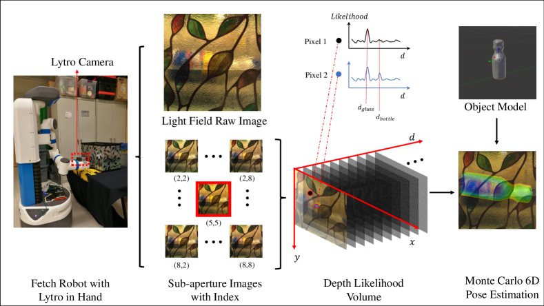
Figure 2: An overview of our Plenoptic Monte Carlo Localization framework. A light field camera is installed on the end effector of the robot. After taking a single shot light field image of the scene, sub-aperture images are extracted (center view highlighted in red). The depth likelihood volume (DLV) is then computed as a 3D array of depth likelihoods over certain pixels $(i,j)$ for depth $d$. The DLV is a comparator of color and gradient similarity between the center view and other sub-aperture images. Assuming a known geometry and region of interest, the six-DoF object pose is estimated by Monte Carlo Localization over a constructed DLV.

II-B Light Field Photography

The contributions of this paper are founded upon models described by Levoy and Hanrahan [13] for understanding light fields and plenoptic functions. Their seminal paper covers the foundations of capturing light fields from digital imagery and using them to synthesize new viewpoints from arbitary camera positions. Building on this work, microlens-based light field photography [8, 20] has witnessed significant advancements in depth estimation, image refocusing, transparent object recognition, and surface reconstruction.

In computer vision, Maneo et al. [15] proposed “light field distortion features” to capture distortions and recognize transparent objects. Sulc et al. [26] separates diffuse color components from 4D light field imagery to suppress non-lambertian surface’s reflection. Wang et al. [28] introduced a light field occlusion model for accurate recovery of the depth information around the edge where occlusion occurs. Jeon et al. [10] overcome the narrow baseline problem of light field cameras based on the sub-pixel shift method. This method generates accurate depth images even when the displacement of two adjacent sub-aperture images is less than 1 pixel. Our presented methods for PMCL build directly upon ideas in recent work by Goldluecke et al. [11, 29] for 3D reconstruction in multi-translucent environments. This work proposes generating multi-orientation features observed in epipolar plane images generated by a light field imagery, with impressive results for 3D reconstruction in high translucency.

In robotics, Oberlin and Tellex [21] introduced a time lapse approach to capture light for pick-and-place localization with a Rethink Baxter robot. This work demonstrated compelling results for localizing grasp and placement points in scenes with transparency and reflection, which has been problematic for current sensors. Our PMCL method shares similar aims with more general models of translucency in mind. Further, estimation of six-DoF object pose estimation by PMCL will allow for greater flexibility in planning and executing manipulation actions. We posit PMCL to be readily capable of object tracking from plenoptic observations, although such experiments are left for future work.

III Problem Formulation

Given an input light field image observation $Z$, the purpose of six-DoF pose estimation is to infer the rigid transformation from an object’s local coordinate frame $\mathcal{O}$ to the camera’s coordinate frame $\mathcal{C}$. We assume as given the geometry of the target object $o$. Formally, we aim to find the maximum likelihood estimate for the object’s pose $q$ given $o$ and a map representation $m$ in 3D world coordinates:

$$\arg\max_{q}P(q|m,o)$$ (1)

The map $m$ is often computed as a metric representation, such as a 3D reconstruction or point cloud. In the case of common RGB-D cameras, the map representation is a one-to-one mapping from locations in 3D space $(x,y,z)$ into depth value $d$ at pixel index $(i,j)$ of a depth image. Such a one-to-one mapping assumes opacity in that the sensed depth at a particular pixel is due to light from only one object.

We propose the Depth Likelihood Volume (DLV) as an alternative one-to-many mapping to consider the likelihood of a pixel over multiple levels of depth. As the case for translucent objects, the DLV representation is advantageous in environments where multiple objects at more than one depth are responsible for the light sensed at a pixel. The DLV representation expresses $m$ as the mapping:

$$m:\mathcal{M}_{\rho}(x,y,z)\rightarrow L(i,j,d)$$ (2)

where $\mathcal{M}_{\rho}(x,y,z)$ represents a 3D point $(x,y,z)$ along a light ray $\rho$ taken as input. The output $L(i,j,d)$ is the likelihood of light along the ray $\rho$ emitted from depth $d$ being received by pixel $(i,j)$ in the image plane. For our light field cameras, we assume the image plane is determined by the center view image of the sub-aperture images extracted from light field observation $Z$. $d$ is discretized possible depths along light ray $\rho$. An overview of our approach to this problem is shown in Figure  2.

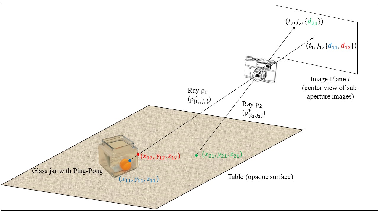
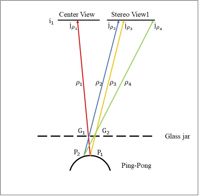
Figure 3: (Left) a scene with a transparent glass jar containing a ping-pong ball at rest on an opaque table. Along ray $\rho_{1}$, two surfaces (incident to the ball and the front surface of the jar) contributes to the pixel value, while along ray $\rho_{2}$ only one surface (incident to the table) appears. (Right) a planar top-down view of rays incident to the ball and the jar. The center view image plane, $(i_{1},j_{\rho_{1}})$ receives a weighted sum of light rays reflected from both the glass surface point $G_{1}$ and the ping-pong surface $P_{1}$. Three example rays corresponding to $\rho_{2}$ (reflection of the surface from the glass jar), $\rho_{3}$ (reflection of the ping-pong ball through the glass), and $\rho_{4}$ (random ray) received by the image plane with incidence to scene points $(G_{1},P_{2})$, $(G_{2},P_{1})$, and $(G_{2},P_{2})$, respectively. They indicate three depth $d_{g},d_{p},d_{i}$ when form stereo pair with ray $\rho_{1}$.

IV Depth Likelihood Volumes

Before presenting our PMCL method for pose estimation, we first define the Depth Likelihood Volume. We describe the properties of the DLV for distinguishing multiple depths at a given point in an image due to translucency. The construction of the DLV and its use for pose localization is described in the following section.

IV-A Formulation

Given a known 3D workspace and its corresponding center view sub-aperture image plane $I$, a Depth Likelihood Volume is defined in Equation 2. The DLV makes the following basic assumptions and notations for the scene:

1. Each surface point emits light rays $\rho$ in each channel as a Gaussian over $(r,g,b)$ with mean $(\mu_{r},\mu_{g},\mu_{b})$ and variance $(\sigma_{r}^{2},\sigma_{g}^{2},\sigma_{b}^{2})$ which means $\rho=\mathcal{N}(\lambda;\mu_{c},\sigma_{c}^{2}),c\in\{r,g,b\}$, as similarly assumed by Oberlin and Tellex [21]. Under constant lighting condition we assume every point in the scene shares the same variance for the same color channel which means $\sigma_{c}=\sigma_{c}^{\prime},c\in\{r,g,b\}$ for all points in the scene.

2. An observed bundle of rays located at pixel plane $(i,j)$ is a linear combination of all light rays emitted by surface points along the light rays with the normalization scalers $\alpha_{i}$. $\alpha_{i}$ indicates the percentage of rays emitted by the surface in observed rays which measures the transparency of the surface, and we have $\sum_{i}\alpha_{i}=1$.

Consider the example in Figure 3 (Left) of two light rays $\rho_{\{i_{1},j_{1}\}}^{v},\rho_{\{i_{2},j_{2}\}}^{v}$ imaged by the central view sub-aperture image. The index $v$ indicates center view, and $\{\cdot,\cdot\}$ are pixel coordinates in the center view. These rays are in the 3D space hitting the center view plane $I$ at $(i_{1},j_{1}),(i_{2},j_{2})$, respectively. Along $\rho_{\{i_{1},j_{1}\}}^{v}$, there are two surfaces emitting light which are sensed by the central view: one is a ping-pong ball and the other is the glass jar. In contrast, along $\rho_{\{i_{2},j_{2}\}}^{v}$, only light emitted by the table is sensed in the central view. Then $\rho_{\{i_{1},j_{1}\}}^{v},\rho_{\{i_{2},j_{2}\}}^{v}$ can be expressed respectively as:

$$\rho_{\{i_{1},j_{1}\}}^{v}=\alpha_{g}\rho_{\textrm{glass}}+\alpha_{p}\rho_{\textrm{ping-pong}}$$ (3)

$$\rho_{\{i_{2},j_{2}\}}^{v}=\alpha_{t}\rho_{\textrm{table}}$$

where $\rho_{\textrm{glass}},\rho_{\textrm{ping-pong}},\rho_{\textrm{table}}$ represents the light rays emitted by glass, ping-pong, and table surfaces, respectively. According to our second assumption, we also have $\alpha_{g}+\alpha_{p}=1$ and $\alpha_{t}=1$.

Then the depth likelihood is defined as:

$$L(i,j,d)=$$ (4)

$$\sum_{n}\frac{\max_{k}||\rho_{\{i,j\}}^{v},\mathcal{T}_{k}^{n}(\rho_{\{i,j\}}^{v})||^{2}-||\rho_{\{i,j\}}^{v},\mathcal{T}_{d}^{n}(\rho_{\{i,j\}}^{v})||^{2}}{\sum_{k}||\rho_{\{i,j\}}^{v},\mathcal{T}_{k}^{n}(\rho_{\{i,j\}}^{v})||^{2}}$$

where $\mathcal{T}_{k}^{n}(\rho_{\{i,j\}}^{v})$ is the transformation function finding the light ray corresponding to $\rho_{\{i,j\}}^{v}$ in stereo pair image index with $n$ that indicates depth $k$ . For light field camera known baseline $b$ and focal length $f$, the $\mathcal{T}_{k}^{n}(\cdot)$ can be expressed as $\frac{bf}{D}$, where $D$ is disparity which is the function of $n$ and $k$. $||\cdot,\cdot||^{2}$ is the squared similarity distance between two light rays over $\{r,g,b\}$ color space which is defined as $L_{2}$ distance between two Gaussian mixture models according to assumption (1) and (2) and can be expressed as Equation 9.

IV-B Validity

We claim that for a given $(i,j)$ in DLV the following Lemma holds:

Lemma 1

$$\alpha_{1}<\alpha_{2}\iff L(i,j,d_{1})<L(i,j,d_{2})$$

where $d_{1},d_{2}$ indicates the true surface depth viewed from center view with transparency indicator $\alpha_{1},\alpha_{2}$. This means, the more transparent a surface, the less likelihood the depth of this surface will be in the DLV.

To show the Lemma 1, we consider the scene as shown in Figure 3 (Right). In the center view (where DLV will be built), $\rho_{\{i,j_{\rho_{1}}\}}^{v}$ (simplify notation as $\rho_{1}$) contains rays from the glass surface point $G_{1}$ and ping-pong surface point $P_{1}$ which has depths $d_{g}$, $d_{p}$ respectively. We then evaluate three possible depths in this scene: $d_{g}$, $d_{p}$, and a invalid depth $d_{i}$. For every surface point, corresponding $\alpha_{g},\alpha_{p},\alpha_{i}$ are set as $\alpha_{g}=\alpha,\alpha_{p}=（1-\alpha）,\alpha_{i}=0$. Notice that $\alpha<0.5$ since glass is a transparent surface while ping-pong is not. Using function $\mathcal{T}_{k}^{n}(\rho_{1})$ we can find three rays ($\rho_{2}$,$\rho_{3}$,$\rho_{4}$) in stereo image $n$ corresponding to three depths $d_{g}$, $d_{p}$, and $d_{i}$ separately. Then, we can write ray $\rho_{1}$ as:

$$\rho_{1}=\alpha\mathcal{N}(\lambda;\mu_{G_{1}c},\sigma_{G_{1}c}^{2})+(1-\alpha)\mathcal{N}(\lambda;\mu_{P_{1}c},\sigma_{P_{1}c}^{2})$$ (5)

where $c\in\{r,g,b\}$ represents three color channels. Without loss of generality, we investigate the red channel and write $\rho_{2},\rho_{3},\rho_{4}$ in same fashion:

$$\rho_{2}=\alpha\mathcal{N}(\lambda;\mu_{G_{1}r},\sigma_{G_{1}r}^{2})+(1-\alpha)\mathcal{N}(\lambda;\mu_{P_{2}r},\sigma_{P_{2}r}^{2})$$ (6)

$$\rho_{3}=\alpha\mathcal{N}(\lambda;\mu_{G_{2}r},\sigma_{G_{2}r}^{2})+(1-\alpha)\mathcal{N}(\lambda;\mu_{P_{1}r},\sigma_{P_{1}r}^{2})$$ (7)

$$\rho_{4}=\alpha\mathcal{N}(\lambda;\mu_{G_{2}r},\sigma_{G_{2}r}^{2})+(1-\alpha)\mathcal{N}(\lambda;\mu_{P_{2}r},\sigma_{P_{2}r}^{2})$$ (8)

Here, we assume that transparent surfaces emit an equal amount of light rays between any two stereo images because the disparity range between adjacent sub-aperture views of the Lytro camera is smaller than $\pm 1$ pixel [30] (around $10^{-4}$ rads in view angle in our experiment setting). The squared similarity ( $||\cdot,\cdot||^{2}$ ) distance between $\rho_{1}$ and any other rays can be expressed as:

$$||\rho_{1}(\lambda),\rho_{n}(\lambda)||^{2}=\int(\rho_{1}(\lambda)-\rho_{n}(\lambda))^{2}\;d\lambda$$ (9)

where $n\in\{2,3,4\}$. Given this general expression of distance, we can now provide explicit expressions for the example shown in Figure 3 Right:

$$||\rho_{1}(\lambda),\rho_{2}(\lambda)||^{2}=2(1-\alpha)^{2}(A-\mathcal{N}(\mu_{P_{1}r};\mu_{P_{2}r},2\sigma_{r}^{2}))$$ (10)

$$||\rho_{1}(\lambda),\rho_{3}(\lambda)||^{2}=2\alpha^{2}(A-\mathcal{N}(\mu_{G_{1}r};\mu_{G_{2}r},2\sigma_{r}^{2}))$$ (11)

$$||\rho_{1}(\lambda),\rho_{4}(\lambda)||^{2} =||\rho_{1}(\lambda),\rho_{2}(\lambda)||^{2}+||\rho_{1}(\lambda),\rho_{3}(\lambda)||^{2}$$ (12)

$$+2\alpha(1-\alpha)(\mathcal{N}(\mu_{G_{1}r};\mu_{P_{1}r},2\sigma_{r}^{2})$$

$$-\mathcal{N}(\mu_{G_{1}r};\mu_{P_{2}r},2\sigma_{r}^{2})$$

$$+\mathcal{N}(\mu_{G_{2}r};\mu_{P_{2}r},2\sigma_{r}^{2})$$

$$-\mathcal{N}(\mu_{G_{2}r};\mu_{P_{1}r},2\sigma_{r}^{2}))$$

where $A=\frac{1}{\sqrt{4\pi\sigma_{r}^{2}}}$ and given the following relation:

$$\int\mathcal{N}(x;\mu,\Sigma)\mathcal{N}(x;\mu^{\prime},\Sigma^{\prime})dx=\mathcal{N}(\mu;\mu^{\prime},\Sigma+\Sigma^{\prime})$$ (13)

For the same object, under $~{}10^{-4}$ rads view difference, we assume the color difference between two surface points have the same scale $\Delta$. This assumption implies, for some small value $\epsilon$, that $\epsilon>\Delta=|\mu_{P1r}-\mu_{P2r}|=|\mu_{G1r}-\mu_{G2r}|$.

Disregarding constant scale $2$, Equation 10, 11, 12 can be simplified as Equation 14, 15, 16:

$$||\rho_{1}(\lambda),\rho_{2}(\lambda)||^{2}=(1-\alpha)^{2}A(1-\exp^{-\frac{\Delta^{2}}{4\sigma_{r}^{2}}})$$ (14)

$$||\rho_{1}(\lambda),\rho_{3}(\lambda)||^{2}=\alpha^{2}A(1-\exp^{-\frac{\Delta^{2}}{4\sigma_{r}^{2}}})$$ (15)

$$||\rho_{1}(\lambda),\rho_{4}(\lambda)||^{2}=((1-\alpha)^{2}+\alpha^{2})A(1-\exp^{-\frac{\Delta^{2}}{4\sigma_{r}^{2}}})$$ (16)

Considering an individual stereo pair and applying Equation LABEL:depth_likelihoos_function, we can now express the DLV values for the possible depths for the surface of ping-pong ball, $d_{p}$, the glass surface, $d_{g}$, and the invalid depth, $d_{i}$, as:

$$L(i,j,d_{p})=\frac{(1-\alpha)^{2}}{(1-\alpha)^{2}+\alpha^{2}}$$ (17)

$$L(i,j,d_{g})=\frac{\alpha^{2}}{(1-\alpha)^{2}+\alpha^{2}}$$ (18)

$$L(i,j,d_{i})=\quad\quad 0$$ (19)

which implies that the ping-pong surface must return more light than the glass surface:

$$\alpha_{g}<\alpha_{p}\iff L(i,j,d_{g})<L(i,j,d_{p}),\alpha_{p},\alpha_{g}\in[0,1]$$ (20)

Therefore, Lemma 1 holds.

IV-C Computation

Our implementation uses the $L_{2}$ distance between adjacent pixel colors to approximate the similarity of rays in stereo pairs, as photosensors are unable to capture the distribution over wavelengths of light. Considering this limitation, a cost-volume stereo comparison method based on sub-pixel shift [9, 10] was implemented. Two different cost volumes were implemented: the sum of $L_{2}$ distance in color space ($C_{c}$) and the sum of gradient differences ($C_{g}$). The cost volume $C$ then can be defined as:

$$C(\mathbf{x}_{\rho},l)=\beta C_{c}(\mathbf{x}_{\rho},l)+(1-\beta)C_{g}(\mathbf{x}_{\rho},l)$$ (21)

where $\mathbf{x}_{\rho}=(i,j)$ describes the image coordinate of ray $\rho$, $l$ is depth labels and $\beta$ is a scalar to weight two parts. The terms $C_{c}$ and $C_{g}$ are defined as:

$$C (\mathbf{x}_{\rho},l)=$$ (22)

$$\sum_{\mathbf{s}\neq\mathbf{s}_{c}}\sum_{\mathbf{x}_{\rho}\in R_{\mathbf{x}}}\min(|I(\mathbf{s}_{c},\mathbf{x}_{\rho})-I(\mathbf{s},\mathbf{x}_{\rho}+\Delta\mathbf{x}(\mathbf{s},l))|,\tau_{1})$$

$$C_{g} (\mathbf{x}_{\rho},l)=$$

$$\sum_{\mathbf{s}\neq\mathbf{s}_{c}}\sum_{\mathbf{x}_{\rho}\in R_{\mathbf{x}}}\gamma\min(|I_{x}(\mathbf{s}_{c},\mathbf{x}_{\rho})-I_{x}(\mathbf{s},\mathbf{x}_{\rho}+\Delta\mathbf{x}(\mathbf{s},l))|,\tau_{2})$$

$$+(1-\gamma)\min(|I_{y}(\mathbf{s}_{c},\mathbf{x}_{\rho})-I_{y}(\mathbf{s},\mathbf{x}_{\rho}+\Delta\mathbf{x}(\mathbf{s},l))|,\tau_{2})$$

where $I$ is the image, $I_{x},I_{y}$ is the image gradient in $x,y$ direction, $R_{\mathbf{x}}$ is a rectangular region that center at $\mathbf{x}_{\rho}$; $\tau_{1},\tau_{2}$ is a truncation value of a robust function, $\Delta\mathbf{x}(s,l)$ is the sub-pixel displacement, and $\gamma=\frac{|\mathbf{s}-\mathbf{s}_{c}|}{|\mathbf{s}-\mathbf{s}_{c}|+|\mathbf{t}-\mathbf{t}_{c}|}$ weights different sub-aperture’s gradient contributions to the center view image. Variables $\mathbf{s},\mathbf{t}$ represent pixel in sub-aperture image index coordinate and $\mathbf{s}_{c},\mathbf{t}_{c}$ represent pixel in the center view.

For a certain depth label $l_{i}$, the depth likelihood can be expressed as below based on Equation LABEL:depth_likelihoos_function:

$$L(\mathbf{x}_{\rho},l_{i})=\log(\frac{\arg\max_{l}C(\mathbf{x}_{\rho},l)-C(\mathbf{x}_{\rho},l_{i})}{\sum_{l_{i}}(C(\mathbf{x}_{\rho},l_{i}))}+1)$$ (23)

Optionally, to further distinguish possible depths, the DLV can be truncated by finding $N_{lm}$ number of local maximum with its $K_{lm}$ number of neighbors and setting the other depth likelihoods to $0$.

V Plenoptic Monte Carlo Object Localization

Building on the DLV, we now describe our method of object pose estimation as Plenoptic Monte Carlo Localization. PMCL employs particle filtering to estimate the pose of target objects from the computed DLV. PMCL takes direct inspiration from the work of Dellaert et al. [6] for approximate inference in the form of a sequential Bayesian filter,

$$Bel(q_{t})\propto p(z_{t}|q_{t})\sum_{j}p(q_{t}^{(j)}|q_{t-1}^{(j)})Bel(q_{t-1}^{(j)})$$ (24)

where a collection of $n$ weighted particles $\{q_{t}^{(j)},w_{t}^{(j)}\}_{j=1}^{n}$ is used to represent the pose belief $q_{t}$.

Each particle ${q_{t}^{(j)}}$ is a hypothesized six-DoF pose of the object and is associated with the weight ${w_{t}^{(j)}}$ indicating how likely the sample is to be close to the actual pose. The initial samples are generated by uniformly sampling the six-DoF pose with identical weight. The weight of each sample is then calculated by using the observation likelihood function described in the next paragraph. With the computed weights, an importance sampling with resampling procedure is performed to concentrate hypothesized particles to more weighted range. For state transition, each particle will be perturbed by a zero-mean Gaussian distribution in the space of six-DoF in the action model. This inference can be naturally extended to the case of tracking with an explicit action model and observations over time. In our implementation, the process will iteratively repeat until the average weight is above a chosen threshold for taking an estimate.

Our likelihood function measures the score of a sample’s rendered depth image for a scene DLV. The z-buffer of a 3D graphics engine is used to render each sample into a depth image for comparison with the observation. This rendered depth image, represented as $z^{(j)}$, is mapping back to DLV to find the corresponding depth likelihood interval $[l_{n},l_{m})$. Here, we use an interval because the rendered depth value for a certain pixel may not exactly match its discretized depth value. After finding the corresponding interval, the depth likelihood is calculated using linear interpolation:

$$L(\mathbf{x}_{\rho},l_{n})=L(\mathbf{x}_{\rho},l_{n})+\frac{(l-l_{n})(L(\mathbf{x}_{\rho},l_{m})-L(\mathbf{x}_{\rho},l_{n}))}{l_{m}-l_{n}}$$ (25)

For the rendered image, with every rendered pixel having non-zero (vaild) depth value $l_{i}$, the score for this depth image can be expressed as:

$$L(z_{t})=\frac{\sum_{i}L(\mathbf{x}_{\rho},l_{i})}{N}$$ (26)

where $N$ is the number of valid depths in the rendered image.

VI Results

We now present results for our implementation of PMCL for object localization and grasping in environments with different forms of translucency. We have implemented PMCL using observations from a Lytro light field camera mounted on the wrist of a Michigan Progress Fetch robot (Figure 4). These results consider pick-and-place grasping in two types of scenes with: 1) a single transparent object with an opaque but possible reflective background objects (Figures 5a,  5b), and 2) opaque objects behind translucent non-transparent surfaces (Figures 5c,  5d).

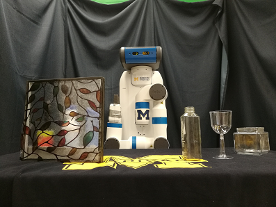
Figure 4: Test objects for evaluating PMCL 6D pose estimation include: (to the left) opaque objects behind a partially opaque translucent surface (a stained glass window film), and (to the right) transparent objects.

Our implementation uses the Lytro on-chip wifi to trigger the shutter remotely and receive raw image data. We are currently unable to capture video with this triggering system. Calibration and sub-aperture images are generated using the methods described by Bok et al. [2]. This toolbox generates $9\times 9$ sub-aperture images, where the image at index $(5,5)$ is deemed the center view image. Each sub-aperture image has resolution $328\times 328$. During DLV construction, we disregard edge sub-aperture images due to strong color distortion and pixel shifting artifacts.

Our PMCL algorithm is implemented on CUDA and OpenGL. This implementation ran on a Ubuntu 14.04 operating system with a Titan X graphics card and CUDA 8.0. The light field camera calibration, sub-aperture images extraction, and DLV construction ran in MATLAB. The chosen parameters for building the DLV were $\beta=0.5$, $\tau_{1}=0.5$, $\tau_{2}=0.5$, $l=75$, $N_{lm}=2$, and $K_{lm}=2$. The Monte Carlo localization process ran on the GPU with 100 particle samples over 500 iterations. With an assumed object geometry, our implementation renders all the particle hypotheses on the GPU. These renderings can be accessed by the CUDA kernels to compute the corresponding weights. Our implementation additionally assumes a given 3D region of interest on the object pose in workspace.

For robot control, we use our custom manipulation pipeline developed by the Laboratory for Progress. This pipeline uses our implementation of handle grasp localization as proposed by ten Pas and Platt [27]. This grasp localization returns an end-effector pose for grasping from an estimated object pose with a given geometric model. Grasping is then executed for this end-effector pose using TRAC-IK [1] and MoveIt! [23] for inverse kinematics and motion planning.

(a)

(b)

(c)

(d)

Figure 5: Two types of scene for localizing object poses. (a-b) the scene with a single transparent object with an opaque but possible reflective background objects. (c-d) the scene with opaque objects behind translucent non-transparent surfaces

To evaluate the pose estimation accuracy of our algorithm, we used two methods to collect ground-truth object poses. For objects behind the window covered by stained glass film, we captured point clouds by removing the glass and using Asus Xtion Pro RGB-D on the robot. Object models were then fit manually to determine ground truth pose values. For transparent objects, their surfaces were covered with opaque tape to generate point clouds for ground truth annotation.

(a)

(b)

Figure 6: The percentage of correctly localized object under different thresholds for the object behind a stained glass panel and a single transparent object. In each plot, the translation error bound is fixed to 1cm (a) and 2cm (b). The x-axis is the decreasing dot product bound indicate the error between ground truth and estimated result. The y-axis is the percentage of correctly localized objects. For each type of scene, these plots consider two types of rotation error ranges: $[0,1]$ in dot product space indicates for [90,0] in degrees, and the absolute value [-1,1] in dot product space indicates [180, 0] in degrees.

VI-A Pose Estimation Results

We evaluate our proposed algorithm on six scenes and run ten trials for each. Two types of error are applied to evaluate our pose estimation accuracy:

• Translation error: defined as the Euclidean distance between estimated object position $(x,y,z)$ and ground truth position $(x_{gt},y_{gt},z_{gt})$

• Rotation error: defined as dot product between ground truth pose z-axis and estimated pose z-axis. We assume the objects are rotational symmetric along z-axis.

We consider an object is correctly localized when both translation and rotation errors fall into a certain threshold. Figure 6 establishes our estimation accuracy on two types of the scene. For the single transparent object, the all rotation error in dot product space laid in [0,1], which leads to the overlapping of yellow and purple lines in both plots. For an object behind stained glass panels, the estimated poses sometimes have 180 degree flipping, a negligible form of error assuming symmetry.

VI-B Manipulation Results

We succeed in demonstrating our method in two challenge scenarios for manipulation,

1. Pick-and-place glass cup from a sink with running water

2. Pick-and-place bleach bottle from an aquatic tank covered with private window film.

The scenarios are shown in Figure 1 and Figure 7. We attach the Lytro camera to the wrist of the robot and add extra link for it. For both scenarios, the robot moves its arm to the appropriate area to capture the light field images, from which the DLV is calculated. Our PMCL then performs estimation to infer the pose of the object and the final estimation is taken to transform the pre-calculated grasp poses in robot base link. With the accurate pose estimation, the robot is able to pick up objects from both aquatic tank and sink and place the objects on the desired location.

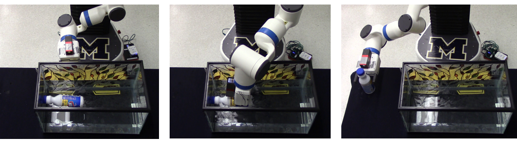
Figure 7: The robot executes pick-and-place action for the bleach bottle floating on the water. The bleach bottle is inside the aquatic tank so it is occluded by the stained glass from the camera view.

VII Conclusion

In this paper, we present Plenoptic Monte Carlo Localization for localizing object pose in the presence of translucency from plenoptic (light-field) observations. We propose a new depth descriptor, the Depth Likelihood Volume, to address the uncertainties from the translucency by generating possible depth likelihoods for each pixel. We show that by using the Depth Likelihood Volume within a Monte Carlo object localization algorithm our method is able to accurately localize objects with translucent materials and objects occluded by layered translucency and perform manipulation.

References

- [1] P. Beeson and B. Ames. Trac-ik: An open-source library for improved solving of generic inverse kinematics. In IEEE-RAS International Conference on Humanoid Robots, 2015.
- [2] Y. Bok, H.-G. Jeon, and I. S. Kweon. Geometric calibration of micro-lens-based light field cameras using line features. IEEE transactions on pattern analysis and machine intelligence, 39(2):287–300, 2017.
- [3] M. Borga and H. Knutsson. Estimating multiple depths in semi-transparent stereo images. 1999.
- [4] M. Ciocarlie, K. Hsiao, E. G. Jones, S. Chitta, R. B. Rusu, and I. A. Şucan. Towards reliable grasping and manipulation in household environments. In Experimental Robotics, pages 241–252. Springer Berlin Heidelberg, 2014.
- [5] A. Collet, M. Martinez, and S. S. Srinivasa. The moped framework: Object recognition and pose estimation for manipulation. Int. J. Rob. Res., 30(10):1284–1306, Sept. 2011.
- [6] F. Dellaert, D. Fox, W. Burgard, and S. Thrun. Monte carlo localization for mobile robots. In IEEE International Conference on Robotics and Automation (ICRA 1999), May 1999.
- [7] P. Foster, Z. Sun, J. J. Park, and B. Kuipers. Visagge: Visible angle grid for glass environments. In Robotics and Automation (ICRA), 2013 IEEE International Conference on, pages 2213–2220. IEEE, 2013.
- [8] T. Georgiev, Z. Yu, A. Lumsdaine, and S. Goma. Lytro camera technology: theory, algorithms, performance analysis. In Multimedia Content and Mobile Devices, volume 8667, page 86671J. International Society for Optics and Photonics, 2013.
- [9] A. Hosni, C. Rhemann, M. Bleyer, C. Rother, and M. Gelautz. Fast cost-volume filtering for visual correspondence and beyond. IEEE Transactions on Pattern Analysis and Machine Intelligence, 35(2):504–511, 2013.
- [10] H.-G. Jeon, J. Park, G. Choe, J. Park, Y. Bok, Y.-W. Tai, and I. So Kweon. Accurate depth map estimation from a lenslet light field camera. In Proceedings of the IEEE Conference on Computer Vision and Pattern Recognition, pages 1547–1555, 2015.
- [11] O. Johannsen, A. Sulc, N. Marniok, and B. Goldluecke. Layered scene reconstruction from multiple light field camera views. In S.-H. Lai, V. Lepetit, K. Nishino, and Y. Sato, editors, Computer Vision – ACCV 2016, pages 3–18, Cham, 2017. Springer International Publishing.
- [12] Z. Lei, K. Ohno, M. Tsubota, E. Takeuchi, and S. Tadokoro. Transparent object detection using color image and laser reflectance image for mobile manipulator. In Robotics and Biomimetics (ROBIO), 2011 IEEE International Conference on, pages 1–7. IEEE, 2011.
- [13] M. Levoy and P. Hanrahan. Light field rendering. In Proceedings of the 23rd annual conference on Computer graphics and interactive techniques, pages 31–42. ACM, 1996.
- [14] I. Lysenkov. Recognition and pose estimation of rigid transparent objects with a kinect sensor. Robotics, 273, 2013.
- [15] K. Maeno, H. Nagahara, A. Shimada, and R.-i. Taniguchi. Light field distortion feature for transparent object recognition. In Computer Vision and Pattern Recognition (CVPR), 2013 IEEE Conference on, pages 2786–2793. IEEE, 2013.
- [16] K. McHenry and J. Ponce. A geodesic active contour framework for finding glass. In Computer Vision and Pattern Recognition, 2006 IEEE Computer Society Conference on, volume 1, pages 1038–1044. IEEE, 2006.
- [17] K. McHenry, J. Ponce, and D. Forsyth. Finding glass. In Computer Vision and Pattern Recognition, 2005. CVPR 2005. IEEE Computer Society Conference on, volume 2, pages 973–979. IEEE, 2005.
- [18] V. Narayanan and M. Likhachev. Discriminatively-guided deliberative perception for pose estimation of multiple 3d object instances. In Proceedings of Robotics: Science and Systems, AnnArbor, Michigan, June 2016.
- [19] V. Narayanan and M. Likhachev. Perch: perception via search for multi-object recognition and localization. In Robotics and Automation (ICRA), 2016 IEEE International Conference on, pages 5052–5059. IEEE, 2016.
- [20] R. Ng. Digital light field photography. stanford university California.
- [21] J. Oberlin and S. Tellex. Time-lapse light field photography for perceiving transparent and reflective objects. 2017.
- [22] C. J. Phillips, M. Lecce, and K. Daniilidis. Seeing glassware: from edge detection to pose estimation and shape recovery. In Proceedings of Robotics: Science and Systems, 2016.
- [23] I. A. Sucan and S. Chitta. Moveit! Online Availabl e: http://moveit. ros. org, 2013.
- [24] Z. Sui, L. Xiang, O. C. Jenkins, and K. Desingh. Goal-directed robot manipulation through axiomatic scene estimation. The International Journal of Robotics Research, 36(1):86–104, 2017.
- [25] Z. Sui, Z. Zhou, Z. Zeng, and O. C. Jenkins. Sum: Sequential scene understanding and manipulation. In 2017 IEEE/RSJ International Conference on Intelligent Robots and Systems (IROS), pages 3281–3288, Sept 2017.
- [26] A. Sulc, A. Alperovich, N. Marniok, and B. Goldluecke. Reflection separation in light fields based on sparse coding and specular flow. In Proceedings of the Conference on Vision, Modeling and Visualization, pages 137–144. Eurographics Association, 2016.
- [27] A. ten Pas and R. Platt. Using geometry to detect grasp poses in 3d point clouds. In International Symposium on Robotics Research, 2015.
- [28] T.-C. Wang, A. A. Efros, and R. Ramamoorthi. Occlusion-aware depth estimation using light-field cameras. In Computer Vision (ICCV), 2015 IEEE International Conference on, pages 3487–3495. IEEE, 2015.
- [29] S. Wanner and B. Goldluecke. Reconstructing reflective and transparent surfaces from epipolar plane images. In German Conference on Pattern Recognition, pages 1–10. Springer, 2013.
- [30] Z. Yu, X. Guo, H. Ling, A. Lumsdaine, and J. Yu. Line assisted light field triangulation and stereo matching. In Computer Vision (ICCV), 2013 IEEE International Conference on, pages 2792–2799. IEEE, 2013.