Stable soft extrapolation of entire functions

Abstract.

Soft extrapolation refers to the problem of recovering a function from its samples, multiplied by a fast-decaying window and perturbed by an additive noise, over an interval which is potentially larger than the essential support of the window. To achieve stable recovery one must use some prior knowledge about the function class, and a core theoretical question is to provide bounds on the possible amount of extrapolation, depending on the sample perturbation level and the function prior.

In this paper we consider soft extrapolation of entire functions of finite order and type (containing the class of bandlimited functions as a special case), multiplied by a super-exponentially decaying window (such as a Gaussian). We consider a weighted least-squares polynomial approximation with judiciously chosen number of terms and a number of samples which scales linearly with the degree of approximation. It is shown that this simple procedure provides stable recovery with an extrapolation factor which scales logarithmically with the perturbation level and is inversely proportional to the characteristic lengthscale of the function. The pointwise extrapolation error exhibits a Hölder-type continuity with an exponent derived from weighted potential theory, which changes from 1 near the available samples, to 0 when the extrapolation distance reaches the characteristic smoothness length scale of the function. The algorithm is asymptotically minimax, in the sense that there is essentially no better algorithm yielding meaningfully lower error over the same smoothness class.

When viewed in the dual domain, soft extrapolation of an entire function of order 1 and finite exponential type corresponds to the problem of (stable) simultaneous de-convolution and super-resolution for objects of small space/time extent. Our results then show that the amount of achievable super-resolution is inversely proportional to the object size, and therefore can be significant for small objects. These results can be considered as a first step towards analyzing the much more realistic “multiband” model of a sparse combination of compactly-supported “approximate spikes”, which appears in applications such as synthetic aperture radar, seismic imaging and direction of arrival estimation, and for which only limited special cases are well-understood.

1. Introduction

1.1. Background

Consider a one-dimensional (in space/time) object $F$, and suppose it is corrupted by a low-pass convolutional filter $K$ and additive modeling/noise error $E$, resulting in the output $G$:

$$G\left(x\right)=\int K\left(x-y\right)F\left(y\right)dy+E\left(x\right).$$

In the Fourier domain, we have

$$\hat{F}(\omega):=\int_{\mathbb{R}}F(x)\exp(-i\omega x)dx$$ (1.1)

and consequently

$$\hat{G}\left(\omega\right)=\hat{K}\left(\omega\right)\hat{F}\left(\omega\right)+\hat{E}\left(\omega\right),$$ (1.2)

where $\hat{K}\left(\omega\right)$ has small frequency support $\Omega_{*}$, the so-called “effective bandlimit” of the system (for example as in the case of the ideal low-pass filter $\hat{K}=\chi_{\left[-\Omega_{*},\Omega_{*}\right]}$). The problem of computational super-resolution asks to recover features of $F\left(x\right)$ from $G\left(x\right)$ below the classical Rayleigh/Nyquist limit $\frac{\pi}{\Omega_{*}}$ [5, 23]. As an ill-posed inverse problem, super-resolution can be regularized using some a-priori information about $F$. One of the main theoretical questions of interest is to quantify the resulting stability of recovery.

Viewed directly in the frequency domain, super-resolution is equivalent to out-of-band extrapolation of $\hat{F}\left(\omega\right)$ for $\left|\omega\right|>\Omega_{*}$ from samples of $\hat{G}\left(\omega\right)$. Since the Fourier transform is an analytic function, this leads to the the problem of stable analytic continuation, widely studied during the last couple of centuries (Subsection 1.3).

1.2. Contributions

In this paper we consider the question of stable extrapolation of certain class of entire functions $\hat{F}$. In more detail, we assume that $\hat{F}$ is analytic in ${\mathbb{C}}$ and, for some $\tau>0$,

$$\sup_{|z|>0,\;z\in{\mathbb{C}}}\left|\hat{F}\left(z\right)\right|\exp\left(-\tau\left|z\right|\right)\leq 1.$$ (1.3)

The underlying motivation for choosing such a growth condition is that the resulting set contains Fourier transforms of distributions of compact support (see Subsection 1.5 below for more details). Another common name for such $\hat{F}$ would be “bandlimited” (or, in this case, “time-limited”).

Furthermore, instead of the “hard” cutoff $\hat{K}=\chi_{\left[-\Omega_{*},\Omega_{*}\right]}$ we consider “soft” windows of super-exponentially decaying shapes, parametrized by $\alpha\geq 2$ (see Figure 1.1c on page 1.1c)

$$\hat{K}\left(\omega\right)=w_{\alpha}\left(\omega\right):=\exp\left(-\left|\omega\right|^{\alpha}\right).$$ (1.4)

Gaussian point-spread functions are considered a fairly reasonable approximation in microscopy [39], and when $\alpha$ is increased the shape of $\hat{K}$ approaches the ideal filter. We therefore argue that the assumption (1.4) is realistic in applications.

We further assume that the perturbation $\hat{E}\left(\omega\right)$ in (1.2) is a uniformly bounded function

$$\left|\hat{E}\left(\omega\right)\right|\leq\varepsilon,\;\omega\in\mathbb{R}.$$ (1.5)

The “soft extrapolation” question, schematically depicted in Figure 1.1a on page 1.1a is then to recover $\hat{F}\left(\omega\right)$ in a stable fashion, over an interval $|\omega|\leq\Omega^{\prime}$ which is potentially larger than the effective support of the window $|\omega|\leq\Omega_{*}$, where both $\Omega^{\prime}$ and $\Omega_{*}$ may depend on $\varepsilon$ and $\alpha,\tau$.

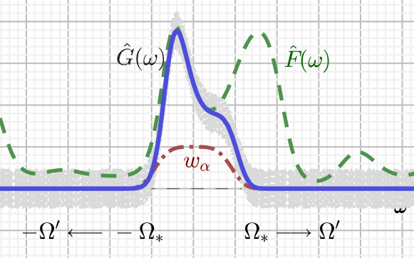
(a) Schematic spectrum extrapolation from noisy and bandlimited data. The original function is $\hat{F}$ (green, dashed). After being multiplied by the window $\hat{K}=w_{\alpha}$ (brown, dash-dot), it gives the blue, solid curve. Adding a corruption $\hat{E}$ of size $\varepsilon$, this gives the data $\hat{G}$ (shaded grey). The question is to recover $\hat{F}(\omega)$ over as wide an interval as possible, with as good an accuracy as possible.

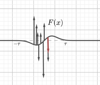
(b) The object prior: the function $F$ has small space/time extent.

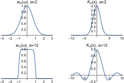
(c) The super-exponentially decaying windows $\hat{K_{\alpha}}(\omega)=w_{\alpha}(\omega)$ (left column) and their inverse Fourier transforms (time domain filters $K_{\alpha}(x)$).

Figure 1.1. The schematic representation of the “soft extrapolation” problem.

Our first main result, Theorem 2.1 below (in particular see also Remark 2.2), shows that a weighted least-squares polynomial approximation with sufficiently dense samples of the form (1.2), taken inside the interval $\left[-\Omega_{*},\Omega_{*}\right]$ with $\Omega_{*}$ scaling (up to sub-logarithmic factors) like $\left(\log{1\over\varepsilon}\right)^{1\over\alpha}$ and a judiciously chosen number of terms achieves an extrapolation factor $\Omega^{\prime}\over\Omega_{*}$ which scales (again, up to sub-logarithmic in $1\over\varepsilon$ factors) like ${1\over\tau}\bigl{(}\log{1\over\varepsilon}\bigr{)}^{1-{1\over\alpha}}$, while the pointwise extrapolation error exhibits a Hölder-type continuity, morally of the form $\varepsilon^{\gamma(\omega)}$ for $|\omega|<\Omega^{\prime}$. The exponent $\gamma$ varies from $\gamma(0)=1$ to $\gamma(\Omega^{\prime})=0$, has an explicit form originating from weighted potential theory, and has itself a minor dependence on $\varepsilon$ that we make explicit in the sequel.

Our second main result, Theorem 2.2 below, shows that the above result is minimax in terms of optimal recovery and thus cannot be meaningfully improved with respect to the asymptotic behaviour in $\varepsilon\ll 1$.

In fact, we prove more general estimates, which hold for functions $\hat{F}$ of finite exponential order $\lambda\geq 1$ and type $\tau>0$, satisfying

$$\sup_{|z|>0}\left|\hat{F}(z)\right|\exp\left(-\tau|z|^{\lambda}\right)\leq 1$$ (1.6)

provided that the window parameter satisfies $\alpha>\lambda$.

1.3. Novelty and related work

Analytic continuation is a very old subject since at least the times of Weierstraß [16]. It is the classical example of an ill-posed inverse problem, and has been considered in this framework since the early 1960’s [33, 34, 10, 35], [6, 7, 19], and more recently [12] and [42]. These works establish regularized linear least squares as a near-optimal computational method, while also deriving the general form of Hölder-type stability, logarithmic scaling of the extrapolation range and the connection to potential theory. Weighted approximation of entire functions has been previously considered in [26, 28]. Below we outline some of these results in more detail, and relate them to ours.

1. Miller [34] and Miller&Viano [35] considered the problem of analytic continuation in the general framework of ill-posed inverse problems with a prescribed bound. A general stabiliy estimate of the form $\varepsilon^{w(z)}$ was established using Carleman’s inequality, and regularized least squares (also known as the Tikhonov-Miller regularization) was shown to be a near-optimal recovery method. The setting in these work is one of “hard” extrapolation, where $F$ is analytic in an open disc $D$, is being measured on a compact closed curve $\Gamma\subset D$, and extended into $D$. It is assumed that $F$ is uniformly bounded by some constant on $\partial D$.

   In contrast, we consider analytic continuation of entire functions satisfying (1.6) on unbounded domains from samples on intervals of the form $\Gamma=\left[-\Omega_{*},\Omega_{*}\right]$ into $D=\{|z|\leq\Omega^{\prime}\}$ where both $\Omega_{*}$ and $\Omega^{\prime}$ can be arbitrarily large when $\varepsilon\ll 1$. It doesn’t appear obvious how to extend the methods in [34, 35] to this setting, without using tools of weighted approximation of entire functions which were developed later.

2. Tikhonov-Miller theory was applied in the particular context of super-resolution in  [6]. The inverse problem of “optical image extrapolation”, i.e. restoring a square-integrable bandlimited function from its measurments on a bounded interval is precisely dual to extrapolating the Fourier transform of a space-limited object of finite energy. For the “hard window” $\chi_{\left[-1,1\right]}$ and any bandlimit $c>0$ the authors showed that the best possible reconstruction error has a Hölder-type scaling $\varepsilon^{\alpha}$ for some $0<\alpha<1/2$, in the uniform norm.

   In contrast, we consider the “soft” formulation, where the convolutional kernel $\hat{K}$ does not vanish, but rather becomes exponentially small at high frequencies. Our estimates give point-wise error bounds so that the Hölder exponent is a function of the particular point, while also providing the functional dependence on the bandlimit $c$ (corresponding to $\tau$ in our notations).

3. Out-of-band extrapolation for bandlimited functions was also considered in [19]. This setting is closely related to ours as the sampling interval can be arbitrary. It was shown that in this case, the optimal extrapolation length scales logarithmically with the signal-to-noise ratio, however no pointwise estimates were obtained. The sampling widow was again the “hard” one $\hat{K}=\chi_{\left[-\Omega,\Omega\right]}$.

   Our results provide a more complete extrapolation scaling, $\tau^{-1}\log{1\over\varepsilon}$ rather than just Landau’s $\log{1\over\varepsilon}$, while also giving pointwise error estimates. We also allow for functions of exponential order $\lambda\geq 1$, and taking $\alpha\to\infty$ and $\lambda=1$, we in fact recover Landau’s scalings.

4. A recent work by Demanet&Townsend [12] investigates the question of stable extrapolation of analytic functions having convergent Chebyshev polynomial expansions in a Bernstein ellipse with parameter $\rho$ from equispaced data on $\left[-1,1\right]$. Linear least squares reconstruction is shown to be asymptotically optimal, if the number of samples scales quadratically with $M$, the number of terms in the approximation, and also $M\sim\log{1\over\varepsilon}$. The resulting extrapolation error scales as $\varepsilon^{\alpha(x)}$ where $\alpha$ has a simple dependence on $\rho$. Naturally, the maximal extrapolation extent is the boundary of the ellipse, i.e. $x_{max}={(\rho+\rho^{-1})\over 2}$, and also $\alpha(1)=1$, while $\alpha(x_{max})=0$.

   Our results are close in spirit to [12], in particular the scaling $\mathfrak{n}\approx\log{1\over\varepsilon}$ for the polynomial approximation order, however the specific setting of soft extrapolation is different. Furthermore, we do not require equispaced samples (but only bound the sample density), and also we obtain point-wise extrapolation error bounds on the entire complex plane rather than just the real line.

5. In another related recent work [42], Trefethen considers stable analytic continuation from an interval $E$ to an infinite half-strip (the so-called “linear” geometry), and shows an exponential loss of significant digits as function of distance from $E$ (corresponding to a stability estimate of the form $\varepsilon^{\alpha(x)}$ where $x$ is the distance from $E$ and $\alpha$ decreases exponentially). In contrast, we consider functions analytic in the entire plane ${\mathbb{C}}$ which is not conformally equivalent to the linear geometry.

6. Extrapolation is closely related to approximation, and in our case of “soft window”, one is naturally lead to adding a corresponding weight function. Indeed, the theory of weighted approximation (in particular of entire functions, [26, 27, 28]) plays a crucial role in our developments. In addition to extending these works to the extrapolation setting, our numerical approximation scheme in this paper does not necessarily require construction of quadrature formulas and orthogonal polynomials with respect to the weight $w_{\alpha}^{2}$.

1.4. Organization of the paper

In Section 2 we define the basic notation and formulate the main theorems. In Section 3 we present some numerical experiments which demonstrate the results in the case of $\alpha=2$ and $\lambda=1$. In Section 4 we quote results from weighted approximation theory which are subsequently used in Section 5 for the proofs.

1.5. Discussion

When viewed in the dual domain (the $x$ variable in (1.1)), soft extrapolation of an entire function of order $\lambda=1$ and finite exponential type $\tau>0$ corresponds to the problem of (stable) simultaneous de-convolution and super-resolution for objects $F$ of small space/time extent $\tau$. Indeed, if $F\in L^{1}$, $\|F\|_{1}\leq 1$, $F$ is even, and $F(t)=0$ if $|t|>\tau$, then the Fourier transform $\hat{F}$ in (1.1) is an entire function satisfying (1.3) (another common name for $\hat{F}$ would be “bandlimited”, although in this case it would be more appropriate to say “time-limited”). This is an example of theorems of Paley-Wiener type ([41, Sect. 7.2], see also [37, p.12]), which hold also for more general classes such as tempered distributions.

In various applications such as seismic imaging, communications, radar, and microscopy, a fairly realistic prior on $F$ takes the form of a sparse atomic combination of compactly supported waveforms, also known as the multiband model in the literature [45, 36, 18, 43]

$$F\left(x\right)\sim\sum_{j=1}^{R}F_{j}\left(x-x_{j}\right),$$ (1.7)

where each $F_{j}\left(x\right)$ is assumed to have a small space/time support but is otherwise unknown. While there exist numerous studies of multiband signals such as the ones quoted above, super-resolution properties associated with this model are not well-understood, except in only some special cases (see e.g. [1, 2, 3, 4, 8, 9, 11, 13, 14, 22, 25, 29, 38, 40] as a very small sample).

Our results in this paper may be interpreted in this context when instead of the sparse sum in (1.7) we can consider the limit of a single object (possibly a distribution) $F$ of compact space/time support $\tau>0$ (Figure 1.1b on page 1.1b). In particular, we obtain the best possible scalings for stability of this inverse problem, showing that the amount of achievable super-resolution scales like ${1\over\tau}\log{1\over\varepsilon}$, and therefore can be significant for small objects with $\tau\ll 1$. Furthermore, a simple algorithm — linear least squares fitting — is asymptotically optimal.

2. Optimal extrapolation of entire functions

2.1. Notation

In the sequel, we fix $\alpha\geq 2$, and omit its mention from notations except to avoid conflict of notation, and for emphasis. Also, contrary to the introductory section, in the remainder of the paper we denote the extrapolation variable by $x$ instead of $\omega$. The functions $\hat{F}$, $\hat{G}$, $\hat{E}$ will correspond to $f,g$ and $\phi$.

We shall use the standard definitions and notations of the spaces $L^{p}$ for $0<p\leq\infty$ (in this paper with respect to the Lebesgue measure on ${\mathbb{R}}$) and the corresponding norms $\|\cdot\|_{p}$.

Given a function $f:{\mathbb{C}}\to{\mathbb{C}}$, and $\tau>0,\;\lambda\geq 1$ we define

$$|\!|\!|f|\!|\!|_{\tau,\lambda}:=\sup_{|z|>0}|f(z)|\exp(-\tau|z|^{\lambda}).$$ (2.1)

Definition 2.1.

Given $\tau>0,\;\lambda\geq 1$, the class $B_{\tau,\lambda}$ consists of all entire functions $f$, real valued on ${\mathbb{R}}$, and satisfying the condition

$$|\!|\!|f|\!|\!|_{\tau,\lambda}\leq 1.$$ (2.2)

Remark 2.1.

Without loss of generality, in this paper we restrict the considerations to the class $B_{\tau,\lambda}$, although it is a proper subset of the set of entire functions of exponential order $\lambda$ and type $\tau$.

Indeed, for fixed $\lambda,\tau$, any $f$ (real-valued on ${\mathbb{R}}$) of order $\lambda$ and type $\tau$ and any $\tau^{\prime}>\tau$ we have $|\!|\!|f|\!|\!|_{\tau^{\prime},\lambda}<\infty$, and therefore $f=cf_{0}$ for some constant $c$ and $f_{0}\in B_{\tau^{\prime},\lambda}$. Furthermore, if the original $f$ is complex-valued on ${\mathbb{R}}$, one can consider the approximation of its real and imaginary parts separately, without changing the main asymptotic behaviour of the bounds.

Definition 2.2.

When comparing small functions of a small quantity $\varepsilon\to 0$, we shall write $a\left(\varepsilon\right)\lessapprox b\left(\varepsilon\right)$ when there exists $\varepsilon_{0}$, depending on $\alpha,\tau,\lambda$ only, such that for all $c_{1}>0$ (however small), there exists $c_{2}>0$, depending on $\alpha,\tau,\lambda,c_{1}$ such that

$$a(\varepsilon)\leq c_{2}\left({1\over\varepsilon}\right)^{c_{1}/{\log\log{1\over\varepsilon}}}b(\varepsilon),\qquad\varepsilon<\varepsilon_{0}.$$

When both $a\lessapprox b$ and $b\lessapprox a$ we shall sometimes write $a\approx b$.

For $y>0$, $\Pi_{y}$ denotes the class of all algebraic polynomials of degree at most $y$. This is the same as the class of polynomials of degree at most $\lfloor y\rfloor$, but the notation is simplified if we simply interpret $\Pi_{y}$ in this way, rather than writing $\Pi_{\lfloor y\rfloor}$.

2.2. Extrapolation by least squares fitting

Let ${\mathcal{C}}=\{x_{M}<\cdots<x_{1}\}$ be a set of arbitrary real numbers. We observe data of the form

$$g(x)=w_{\alpha}(x)f(x)+\phi(x),\qquad x\in{\mathcal{C}},$$ (2.3)

where $f\in B_{\tau,\lambda}$ and $\phi$ is a function satisfying

$$|\phi(x)|\leq\varepsilon,\qquad x\in{\mathcal{C}}.$$ (2.4)

Given ${\mathcal{C}}$ and $g$ as above, we define the operator $S_{n}$ computing the solution to the following least squares problem of degree $n$:

$$\begin{split}S_{n}(g;{\mathcal{C}}):&=\mathop{\hbox{{arg min}}}_{P\in\Pi_{n}}\sum_{j=1}^{M-1}\left(w_{\alpha}^{-1}(x_{j})g(x_{j})-P(x_{j})\right)^{2}(x_{j}-x_{j+1})w_{\alpha}^{2}(x_{j})\\ &=\mathop{\hbox{{arg min}}}_{P\in\Pi_{n}}\sum_{j=1}^{M-1}\left(g(x_{j})-w_{\alpha}(x_{j})P(x_{j})\right)^{2}(x_{j}-x_{j+1}).\end{split}$$ (2.5)

When clear from the context, we shall omit ${\mathcal{C}}$ and write $S_{n}\left(g\right)$.

Let

$$a_{n}:=\beta_{\alpha}n^{1\over\alpha},\qquad\beta_{\alpha}:=\left\{\frac{2^{\alpha-2}\Gamma(\alpha/2)^{2}}{\Gamma(\alpha)}\right\}^{1/\alpha}.$$ (2.6)

Our first main result below bounds the error $|f(z)-S_{n}(g)(z)|$ for $z\in{\mathbb{C}}$ with the particular choice

$$n=\mathfrak{n}(\varepsilon,\alpha,\tau,\lambda)=\biggl{\lfloor}{1\over q(\varepsilon,\alpha,\tau,\lambda)}\log{1\over\varepsilon}\biggr{\rfloor}$$

with $q(\varepsilon)\approx\log\log{1\over\varepsilon}$, under the assumption that the sampling set ${\mathcal{C}}$ approximately lies in the interval $\left[-a_{\mathfrak{n}},a_{\mathfrak{n}}\right]$ and is sufficiently dense.

The error bound heuristically behaves like a $z$-dependent fractional power of the perturbation, but in reality it is slightly more complicated. In more detail:

1. There is a natural rescaling of the $z$ variable by a factor of $a_{\mathfrak{n}}$ (which in turn depends on $\varepsilon$), because the sampling set ${\mathcal{C}}$ and the resulting approximating polynomial $S_{\mathfrak{n}}$ themselves depend on $\mathfrak{n}$. So instead of bounding $|f(z)-S_{n}(g)(z)|$ directly, we have a bound of the form

   $$|f(a_{\mathfrak{n}}z)-S_{\mathfrak{n}}(g)(a_{\mathfrak{n}}z)|\lessapprox\varepsilon^{\gamma(z)}.$$

2. The exponent $\gamma(z)$ in fact has a weak dependence on $\varepsilon$, and it is of the form $\gamma(z)=1-\frac{1}{q(\varepsilon)}\delta(z)$ where $q(\varepsilon)\approx\log\log{1\over\varepsilon}$ is the same function used in the definition of $\mathfrak{n}$ above and $\delta(z)$ is a certain logarithmic potential.

There are three distinct regions in the complex plane with respect to the error asymptotics:

1. The “approximation region” $\left[-a_{\mathfrak{n}},a_{\mathfrak{n}}\right]$. In the range $[-1,1]$ we have in fact $\delta(x)=|\beta_{\alpha}x|^{\alpha}$, and therefore (disregarding the rounding effects) it can be easily shown that

   $$\varepsilon^{\gamma(x)}=\varepsilon w_{\alpha}^{-1}(a_{\mathfrak{n}}x).$$

   This is the error that would be obtained by conventional deconvolution, i.e. division by $w_{\alpha}$. Note that for any $x\in[-1,1]$ we have as $\varepsilon\to 0$

   $$\gamma(x)=1-{\delta(x)\over q(\varepsilon)}\to 1.$$

2. The “extrapolation region”, where the error $\varepsilon^{\gamma(z)}$ is less than $\exp(\tau|a_{\mathfrak{n}}z|^{\lambda})$, i.e. the maximal growth rate for any function in $B_{\tau,\lambda}$. It turns out that the maximal extrapolation interval can be precisely determined as $|z|\leq r_{\mathfrak{n}}/a_{\mathfrak{n}}$, where

   $$r_{n}:=\biggl{(}\frac{n}{\tau\lambda}\biggr{)}^{\frac{1}{\lambda}}.$$

   In terms of the Hölder exponent $\gamma$, it turns out that $\lim_{\varepsilon\to 0}\frac{\delta(r_{\mathfrak{n}}/a_{\mathfrak{n}})}{q(\varepsilon)}=1$, and therefore as $\varepsilon\to 0$ we have

   $$\gamma(r_{\mathfrak{n}}/a_{\mathfrak{n}})\to 0.$$

3. The “forbidden” region $|z|>r_{\mathfrak{n}}/a_{\mathfrak{n}}$ where essentially no information can be obtained about $f$ from the samples on $\left[-a_{\mathfrak{n}},a_{\mathfrak{n}}\right]$.

In Figure 2.1 on page 2.1 we show an example for the behaviour of both the exponent $\gamma(z)$ and the complete bound $\varepsilon^{\gamma(z)}$ for different values of $\varepsilon$ and other parameters fixed.

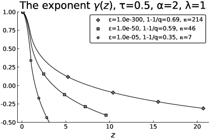
(a) The exponent $\gamma(z)$. As $\varepsilon$ becomes smaller, the values of $\gamma$ in the interval $[0,1)$ approach 1, while at the right boundary $z=r_{\mathfrak{n}}/a_{\mathfrak{n}}$ they approach 0.

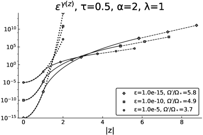
(b) The complete bound $\varepsilon^{\gamma(z)}$ (solid), the quantity $\exp(\tau|a_{\mathfrak{n}}z|^{\lambda})$ (dashed) and $w_{\alpha}^{-1}(a_{\mathfrak{n}}z)$ (dotted).

Figure 2.1. The optimal exponent $\gamma(z)$ and the corresponding error bound $\varepsilon^{\gamma(z)}$ for several values of $\varepsilon$ and $\tau=0.5,\lambda=1,\alpha=2$.

Remark 2.2.

The length of the sampling window $\Omega_{*}$ essentially scales like $a_{\mathfrak{n}}\approx\left({1\over\log\log{1\over\varepsilon}}\log{1\over\varepsilon}\right)^{1\over\alpha}$, while the maximal extrapolation range $\Omega^{\prime}$ is of the asymptotic order $r_{\mathfrak{n}}\approx\left({1\over\tau}{1\over\log\log{1\over\varepsilon}}\log{1\over\varepsilon}\right)^{1\over\lambda}$. Therefore we obtain a genuine extension by a factor of $\Omega^{\prime}/\Omega_{*}\approx\left({1\over\tau}\right)^{1\over\lambda}\left({1\over\log\log{1\over\varepsilon}}\log{1\over\varepsilon}\right)^{{1\over\lambda}-{1\over\alpha}}$.

The result reads as follows, and is proved in Section 5.

Theorem 2.1.

Let $f\in B_{\tau,\lambda}$. For $\varepsilon>0$, $\alpha>\lambda$ let $\mathfrak{n}=\mathfrak{n}(\varepsilon,\alpha,\tau,\lambda)\approx\log\frac{1}{\varepsilon}$ be as defined in (5.45) below. For any sequence of points ${\mathcal{C}}=\left\{x_{M}<\dots<x_{1}\right\}$ satisfying

$$\left[-{4\over 3}a_{\mathfrak{n}},{4\over 3}a_{\mathfrak{n}}\right] \subseteq\left[x_{M},x_{1}\right]\subseteq\left[-2a_{\mathfrak{n}},2a_{\mathfrak{n}}\right],$$ (2.7)

$$|x_{j}-x_{j+1}| \leq c_{1}\mathfrak{n}^{\frac{1}{\alpha}-1},$$ (2.8)

where $c_{1}=c_{1}\left(\alpha\right)$ is the explicit consant defined in (5.52) below, let $S_{\mathfrak{n}}\left(g;{\mathcal{C}}\right)$ be the weighted least squares polynomial fit of degree $\mathfrak{n}$ to $f$ using samples of $g$ as in (2.3), (2.4) and (2.5).

Then the (properly rescaled) pointwise extrapolation error satisfies

$$\left|f\left(a_{\mathfrak{n}}z\right)-S_{\mathfrak{n}}(g)\left(a_{\mathfrak{n}}z\right)\right|\lessapprox\begin{cases}\varepsilon w_{\alpha}^{-1}\left(a_{\mathfrak{n}}z\right)&z\in\left[-1,1\right]\\ \varepsilon^{1-\frac{1}{q\left(\varepsilon\right)}\delta\left(z\right)}&|z|<r_{\mathfrak{n}}/a_{\mathfrak{n}},\;z\in{\mathbb{C}}\\ \exp\left(\tau|a_{\mathfrak{n}}z|^{\lambda}\right)&|z|>r_{\mathfrak{n}}/a_{\mathfrak{n}},\;z\in{\mathbb{C}}\end{cases},$$ (2.9)

where $q\left(\varepsilon\right)$ is given by (5.46) and satisfies $q(\varepsilon)\approx\log\log{1\over\varepsilon}$, while the function $\delta\left(z\right)$ is defined in (5.49) below, such that

$$\lim_{\varepsilon\to 0}\frac{\delta(z)}{q\left(\varepsilon\right)}= 0 |z|$$ for any fixed (2.10)

$$\lim_{\varepsilon\to 0}\frac{\delta(z)}{q\left(\varepsilon\right)}= 1 z=z_{\varepsilon} |z_{\varepsilon}|=r_{\mathfrak{n}}/a_{\mathfrak{n}}$$ for any with . (2.11)

Furthermore, the relation in (2.9) holds uniformly on compact subsets in $z$.

Remark 2.3.

If the points are chosen to be equispaced, then it suffices to have at most linear (in the approximation degree $\mathfrak{n}$) growth of the size of the sampling set ${\mathcal{C}}$, as indeed it is sufficient to take

$$|{\mathcal{C}}_{\textrm{equi}}|={4\over 3c_{1}}a_{\mathfrak{n}}\mathfrak{n}^{1-{1\over\alpha}}\leq c\mathfrak{n}.$$

2.3. Optimality

Next, we will show that the results above cannot be meaningfully improved. To do so, we first review some facts from the theory of optimal recovery based on [32, 31], as they relate to our problem. We consider the set $B_{\tau,\lambda}$ as a subset of the space $X$ of all continuous functions $f:{\mathbb{R}}\to{\mathbb{R}}$ such that $w_{\alpha}f\in L^{\infty}$.

Let $Y$ be a normed linear space with norm given by $\|\cdot\|_{Y}$, and $I:X\to Y$, $R:Y\to X$ be functions. The function $I$ is called information operator, and $R$ is called a recovery operator. In [32, 31], $I$ is required to be a linear operator, but we do not need this restriction here. In its place, we require that

$$\|I(f)\|_{Y}\leq\|w_{\alpha}f\|_{\infty},\qquad f\in X.$$ (2.12)

We give some examples of $R$ and $I$.

1. A trivial example is $Y=X$ and $I(f)=w_{\alpha}f$, $f\in X$. In this case the recovery operator is of interest only for an extension of $f$ to ${\mathbb{C}}$.

2. In this paper, we are considering the mapping $I:X\to{\mathbb{R}}^{M}$ given by

   $$I(f)=(f(x_{M})w_{\alpha}(x_{M}),\cdots,f(x_{1})w_{\alpha}(x_{1})),$$

   and the recovery operator given by $S_{n}$.

3. If $w_{\alpha}f\in L^{1}+L^{\infty}$, we define its Fourier-orthogonal coefficients (see (4.14) below) by

   $$\hat{f}(k)=\int_{\mathbb{R}}f(t)p_{k}(t)w_{\alpha}^{2}(t)dt,\qquad k=0,1,\cdots.$$ (2.13)

   Let $Y$ be the space of all sequences $\{d_{k}\}$ for which

   $$\|\{d_{k}\}\|_{Y}=c_{2}^{-1}\sup_{k\geq 0}(k+1)^{1/(2\alpha)}|d_{k}|<\infty,$$

   where $c_{2}$ is defined in (4.15). The information operator $I(f)=\{\hat{f}(k)\}$ maps $X$ into $Y$, and satisfies (2.12). An example of a recovery operator is the expansion $\sum_{k=0}^{\infty}d_{k}p_{k}(z)$ which converges when $f\in B_{\tau,\lambda}$ and $d_{k}=\hat{f}(k)$. This shows that one can weaken the condition (2.12), allowing a constant factor on the right hand side of the inequality, by renormalizing $Y$.

For any information operator $I$ and recovery operator $R$, $z\in{\mathbb{C}}$, and $\varepsilon>0$, we are interested in the worst case recovery error when the information is perturbed by $\varepsilon$:

$$E(\tau,\lambda,\varepsilon,z;R,I):=\sup_{f\in B_{\tau,\lambda},\;\|y\|_{Y}\leq\varepsilon}|f(a_{\mathfrak{n}}z)-R(I(f)+y)(a_{\mathfrak{n}}z)|,$$ (2.14)

where again $\mathfrak{n}=\mathfrak{n}\left(\varepsilon,\alpha,\tau,\lambda\right)$ as given by (5.45). The best worst case (minimax) error is defined by

$$\mathcal{E}(\tau,\lambda,\varepsilon,z):=\inf_{R,I}E(\tau,\lambda,\varepsilon;R,I),$$ (2.15)

where it is understood that the infimum is over all $R$ and $I$ with all normed linear spaces $Y$, subject to (2.12). Informally, $\mathcal{E}(\tau,\lambda,\varepsilon,z)$ the best accuracy one can expect in reconstructing $f(z)$ for every $f\in B_{\tau,\lambda}$ from any kind of information and recovery based only on the values of $f$ on ${\mathbb{R}}$. It is closely related to the notion of “best possible stablity estimate” of K.Miller [34], cf. Subsection 1.3.

With these notations, the bound (2.9) in Theorem 2.1 means that (with $q=q\left(\varepsilon\right)$ as before)

$$\mathcal{E}(\tau,\lambda,\varepsilon,z)\lessapprox\varepsilon^{1-{1\over q}\delta\left(z\right)},\quad|z|\leq r_{\mathfrak{n}}/a_{\mathfrak{n}}.$$

The following theorem shows that in this sense of optimal recovery, this result is the best possible.

Theorem 2.2.

There exists a function $\xi(\varepsilon)$ satisfying $\xi(\varepsilon)\lessapprox\varepsilon$, such that for any $z\in{\mathbb{C}}$, $\varepsilon>0$

$$\mathcal{E}\left(\tau,\lambda,\xi\left(\varepsilon\right),z\right)\gtrapprox\varepsilon^{1-{1\over q}\delta(z)},$$ (2.16)

the relation holding uniformly for compact sets in the complex plane (w.r.t $z$).

In particular, for any small enough $\varepsilon\ll 1$ there exists a “dark object” $f_{\varepsilon}$ such that

1. for $x\in\left[-\Omega_{*},\Omega_{*}\right]$ it has the same magnitude as the perturbation level:

   $$\left|f_{\varepsilon}\left(x\right)\right|\lessapprox\varepsilon w_{\alpha}^{-1}\left(x\right);$$

2. outside the sampling window, it has the same magnitude as the extrapolation error:

   $$\left|f_{\varepsilon}\left(a_{\mathfrak{n}}z\right)\right|\gtrapprox\varepsilon^{1-{1\over q}\delta\left(z\right)},\qquad|z|\leq r_{\mathfrak{n}}/a_{\mathfrak{n}}.$$

3. A numerical illustration: functions of order $\lambda=1$ with Hermite polynomials

In this section we specialize our preceding results to the case $\alpha=2$, $\lambda=1$, with $f$ a function of finite exponential type $\tau>0$. We then run a simple computational experiment and compare the results with the theoretical predictions, showing good agreement between the two in practice.

For technical convenience, we have chosen to work with an off-the-shelf implementation of Hermite polynomials, which are orthogonal with respect to the weight function $u_{2}(x)=\exp\left(-{x^{2}\over 2}\right)$. So instead of (2.3) we assume that $f$ is blurred by $u_{2}$. Since our weights $w_{\alpha}$ are not of this form, we perform a trivial change of variable $t=x/\sqrt{2}$ and apply our results to the function $h(t):=f(t\sqrt{2})$, which is consequently of exponential type $\tau^{\prime}=\tau\sqrt{2}$.

In this case we have $\beta_{2}=1$, $a_{n}=\sqrt{n}$, $F_{2}=\log(1/2)-1/2$, $v_{2}(t)=(1/\pi)\sqrt{1-t^{2}}$ and also

$$\delta(z)=U(z)-F_{2}=\log\left|z+\sqrt{z^{2}-1}\right|+\Re\left(z^{2}-z\sqrt{z^{2}-1}\right),$$ (3.1)

where the branch of $\sqrt{z^{2}-1}$ is chosen so that $\sqrt{z^{2}-1}/z\to 1$ as $z\to\infty$.

Further, according to our notations, we also have $\rho=\tau^{\prime}\sqrt{e}/2$, $\mu=1/2$ and

$$q\left(\varepsilon\right) ={1\over 2}\mathcal{W}\biggl{(}{4\over\tau^{2}e}\log{1\over\varepsilon}\biggr{)},$$

$$\mathfrak{n} =\left\lfloor{1\over q}\log{1\over\varepsilon}\right\rfloor.$$

To implement the least squares operator $S_{\mathfrak{n}}$, we have chosen to work in the basis of Hermite orthogonal polynomials $H_{n}$ which satisfy $\int H_{k}(x)H_{j}(x)\exp\left(-x^{2}\right)dx=\delta_{k,j}$. Following Remark 2.3 we pick $2\mathfrak{n}$ equispaced samples in $\left[-\sqrt{2\mathfrak{n}},\sqrt{2\mathfrak{n}}\right]$ (i.e. the oversampling factor is $2$).

For running the experiments below, we have chosen the following model function $f_{\tau}$ to extrapolate:

$$f_{\tau}(x):={1\over 14}\bigl{(}5+\cosh\left(\tau x-2\right)+\sinh\left(\tau x\right)\bigr{)}.$$ (3.2)

A simple computation shows that $|\!|\!|f_{\tau}|\!|\!|_{\tau,1}\leq 1$, and therefore $f_{\tau}\in B_{\tau,1}$.

Theorem 2.1 implies that the error satisfies, in the unscaled $z$ variable,

$$|f_{\tau}(z)-S_{\mathfrak{n}}(g)(z)|\lessapprox E_{\tau,\varepsilon}(f;z):=\begin{cases}\varepsilon\exp\left(z^{2}/2\right)&z\in\left[-\sqrt{2\mathfrak{n}},\sqrt{2\mathfrak{n}}\right]\\ \varepsilon^{\gamma^{\prime}_{\varepsilon}(z)},\quad\gamma^{\prime}_{\varepsilon}(z)=1-{1\over q}\delta\left({z\over\sqrt{2\mathfrak{n}}}\right)&|z|\in[\sqrt{2\mathfrak{n}},{\mathfrak{n}\over\tau}]\\ \exp\left(\tau|z|\right)&|z|>{\mathfrak{n}\over\tau}.\end{cases}$$ (3.3)

Instead of the construction used in the proof of Theorem 2.2 (i.e. the function $P_{\mathfrak{n}}^{*}$ given in (5.56)), we shall use the following function as our “dark object” (unrelated to $f_{\tau}$):

$$f_{\tau,\varepsilon}\left(z\right):=\cosh\left(\tau z\right)-\sum_{n<\mathfrak{n}}e^{\frac{\tau^{2}}{4}}\frac{\tau^{n}\pi^{\frac{1}{4}}\left(1+\left(-1\right)^{n}\right)}{\sqrt{2^{n}n!}}H_{n}\left(z\right).$$ (3.4)

It is not difficult to show that this function is in $B_{\sigma,1}$ and in fact also satisfies (5.57) and (5.60). The underlying reason for using a different function $f_{\tau,\varepsilon}$ is that it is not known how to evaluate $P_{\mathfrak{n}}^{*}$ general, while (3.4) is an absolutely explicit formula.

In Figure 3.1 on page 3.1 we show the reconstruction and the corresponding errors + bounds for fixed $\tau,\varepsilon$ in the original scaling. As can be seen in Figure 3.1a on page 3.1a, the derived bounds $E_{\tau,\varepsilon}$ are reasonably accurate. In Figure 3.1b on page 3.1b it is clearly seen that the algorithm chooses a reasonable value for $\mathfrak{n}$, avoiding the extreme noise outside the essential support of the window.

In Figure 3.2 on page 3.2 the reconstruction and comparison were performed for fixed $z_{0}$ and $\sigma$, varying $\varepsilon$. It can be seen that the dependence of the error on $\varepsilon$ is accurately determined. The threshold values of $\varepsilon$ for which one moves from interpolation to extrapolation region ($\varepsilon_{1\to 2}$) and from extrapolation to forbidden region ($\varepsilon_{2\to 3}$) can be approximately determined as the solutions $\varepsilon_{1\to 2}$ and $\varepsilon_{2\to 3}$ of the equations

$$z_{0} =\sqrt{2\mathfrak{n}} \iff \varepsilon_{1\to 2} =\exp\left(-q(\varepsilon_{1\to 2})z_{0}^{2}/2\right),$$ (3.5)

$$z_{0} =r_{\mathfrak{n}} \iff \varepsilon_{2\to 3} =\exp\left(-q(\varepsilon_{2\to 3})\tau z_{0}\right).$$ (3.6)

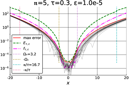
(a) The error and the bounds. Thin black lines are $|f_{\tau}-S_{\mathfrak{n}}(g)(z)|$ for different noise realizations (see (2.3) and (2.4)), their maximal envelope is the red solid curve. The green, dashed curve is the analytical bound $E_{\tau,\varepsilon}$ in (3.3), while the magenta, dashdotted curve is the minimax function $f_{\tau,\varepsilon}$ defined in (3.4). The dotted vertical lines are the region boundaries.

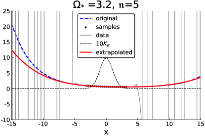
(b) The function (blue dashed) and its extrapolant (red solid). The black dots are the actual sampling points, while the grey curve is the noisy function $u_{2}^{-1}(x)g(x)$ which would need to have been used without extrapolation – recall (2.3). As can be seen, the choice of $\mathfrak{n}$ ensures that the samples are taken inside the essential support of the window, which depends on $\varepsilon$.

Figure 3.1. Results for the function defined in (3.2) with $\tau=0.3$ and $\varepsilon=10^{-5}$.

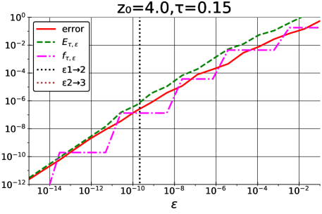
(a) $z_{0}=4$, the transition between regions 1 and 2 (black vertical line) computed numerically from (3.5).

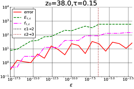
(b) $z_{0}=38$, the transition between regions 2 and 3 (brown vertical line), computed numerically from (3.6).

Figure 3.2. Error (red, solid curve) vs bound $E_{\tau,\varepsilon}$ (green, dashed curve) and the minimax function $f_{\tau,\varepsilon}$ (magenta, dashdotted) from (3.4) for $\tau=0.15$, as function of $\varepsilon$ for a fixed $z_{0}$. Same function $f_{\tau}$ as in (3.2).

4. Preliminaries from weighted approximation theory

4.1. Weighted polynomials

A very important fact in the theory of weighted approximation is that the supremum norm of weighted polynomials is attained on an interval depending only on the degree of the polynomial, and not on the individual polynomials involved. We need to describe this fact in some detail. Let

$$a_{x}(\alpha):=\beta_{\alpha}x^{1/\alpha}:=\left\{\frac{2^{\alpha-2}\Gamma(\alpha/2)^{2}}{\Gamma(\alpha)}\right\}^{1/\alpha}x^{1/\alpha},\qquad x>0,$$ (4.1)

be the so called Mhaskar-Rakhmanov-Saff numbers. The Ullman distribution is defined by

$$v_{\alpha}\left(t\right):=\frac{\alpha}{\pi}\int_{\left|t\right|}^{1}\frac{y^{\alpha-1}}{\sqrt{y^{2}-t^{2}}}dy,\quad\left|t\right|\leq 1.$$ (4.2)

Further denote by $U\left(z\right)$ its logarithmic potential

$$U\left(z\right):=U(\alpha;z)=\int_{-1}^{1}\log\left|z-t\right|dv_{\alpha}\left(t\right),\quad z\in\mathbb{C}.$$ (4.3)

The number

$$F_{\alpha}:=\log(1/2)-\frac{1}{\alpha}$$ (4.4)

is called the modified Robin’s constant for $w_{\alpha}$.

The following is proved in [27, Theorem 6.4.2], in fact, for all $\alpha>0$.

Theorem 4.1.

Let $\alpha>0$. Then

1. The potential $U$ satisfies

   $$\begin{split}U(\alpha;x)=|\beta_{\alpha}x|^{\alpha}+F_{\alpha},&\mbox{ if $x\in[-1,1]$,}\\ U(\alpha;x)<|\beta_{\alpha}x|^{\alpha}+F_{\alpha},&\mbox{ if $x\in{\mathbb{R}}\setminus[-1,1]$.}\end{split}$$ (4.5)

2. If $n>0$, $P\in\Pi_{n}$, then

   $$|P(z)|\leq\exp\left(nU(\alpha;z/a_{n})-nF_{\alpha}\right)\max_{x\in[-a_{n},a_{n}]}|w_{\alpha}P(x)|.$$ (4.6)

   In particular,

   $$\|w_{\alpha}P\|_{\infty}=\max_{x\in[-a_{n},a_{n}]}|w_{\alpha}(x)P(x)|.$$ (4.7)

The following theorem gives an analogue of (4.7) in the case of the $L^{p}$ norms. The proof of this theorem is essentially in [27], but proved in [28, Theorem 2.2] in the form given below.

Theorem 4.2.

Let $1\leq p<\infty$, $\alpha>1$, $a_{x}$ be as in (4.1). For any $\eta>0$, integer $m\geq c\log(1/\eta)$ and $P\in\Pi_{m}$, we have

$$\int_{|y|\geq a_{m}(\alpha)(1+A(\alpha,\eta)/(pm)^{2/3})}|P(y)w_{\alpha}(y)|^{p}dy\leq\eta\|w_{\alpha}P\|_{p}^{p},$$ (4.8)

where

$$A(\alpha,\eta)\geq\left\{\left(\frac{2}{3}\alpha\min(2^{\alpha-2},1/(\alpha-1))\right)^{-1}\left(\log(2/(2-\sqrt{3})^{2})+\log(1/\eta)\right)\right\}^{2/3}.$$ (4.9)

In the sequel, we will use the notation

$$\Delta_{n}(p,\alpha,\eta)=[-a_{n}(\alpha)(1+A(\alpha,\eta)/(pn)^{2/3}),a_{n}(\alpha)(1+A(\alpha,\eta)/(pn)^{2/3})].$$ (4.10)

Definition 4.1.

Let $\mathcal{T}_{n}$ denote the unique monic polynomial of degree $n$ satisfying

$$\|\mathcal{T}_{n}w_{\alpha}\|_{\infty}=\inf_{P\in\Pi_{n-1}}\|\left(\left(\cdot\right)^{n}-P\right)w_{\alpha}\|_{\infty}.$$ (4.11)

These are also called weighted Chebyshev polynomials, as the above expression is completely analogous to the well-known property of the classical Chebyshev polynomials $T_{n}$, namely that $T_{n}$ is the minimax monic approximant to the zero function [15, Theorem 3.6].

The following proposition (see e.g.[27, Section 6.3], [24, Corollary 3.3]) lists some of the required properties of $\mathcal{T}_{n}$.

Proposition 4.1.

Let $\alpha\geq 2$. Then

1. For $n\geq 1$, the polynomial $\mathcal{T}_{n}$ has $n$ simple zeros in $[-a_{n},a_{n}]$: $-x_{n,n}^{*}<\cdots<x_{1,n}^{*}$.

2. We have

   $$\lim_{n\to\infty}\frac{\|\mathcal{T}_{n}w_{\alpha}\|_{\infty}}{a_{n}^{n}\exp(-nF_{\alpha})}=(1/2)e^{-1/\alpha}.$$ (4.12)

3. Uniformly on compact subsets of ${\mathbb{C}}\setminus[-1,1]$, we have

   $$\lim_{n\to\infty}\frac{|\mathcal{T}_{n}(a_{n}z)|}{a_{n}^{n}\exp(-nU(z))}=\lim_{n\to\infty}\frac{|\mathcal{T}_{n}(a_{n}z)|}{\|\mathcal{T}_{n}w_{\alpha}\|_{\infty}\exp(-nU(z)+nF_{\alpha})}=1.$$ (4.13)

We will also use another family of polynomials. Let $\{p_{k}\}_{k=0}^{\infty}$ be the system of orthonormalized polynomials with respect to $w_{\alpha}^{2}$; i.e., for each $k=0,1,\cdots$, $p_{k}(x)=\gamma_{k}x^{k}+\cdots\in\Pi_{k}$, and for $k,j=0,1,\cdots$,

$$\int_{\mathbb{R}}p_{k}(t)p_{j}(t)w_{\alpha}^{2}(t)dt=\left\{\begin{array}[]{ll}1,&\mbox{ if $k=j$,}\\ 0,&\mbox{otherwise.}\end{array}\right.$$ (4.14)

It is known [21, Theorem 13.6] that there exist constants $c_{1},c_{2}>0$ depending only on $\alpha$ such that

$$c_{1}\leq n^{1/(2\alpha)}\|w_{\alpha}p_{n}\|_{1}\leq c_{2}.$$ (4.15)

4.2. Weighted approximation of entire functions

If $1\leq p\leq\infty$ and $w_{\alpha}f\in L^{p}$, we define the degree of approximation of $f$ by

$$E_{n}(p;f)=E_{n}(\alpha,p;f):=\inf_{P\in\Pi_{n}}\|(f-P)w_{\alpha}\|_{p},\qquad n=0,1,2,\cdots.$$ (4.16)

In [27, Theorem 7.2.1(b)], we have proved the following theorem (with a different notation).

Theorem 4.3.

Let $1\leq p\leq\infty$, $\lambda>0$, $\alpha>\lambda$, $w_{\alpha}f\in L^{p}$, and

$$\rho_{1}(\alpha,p;f):=\limsup_{n\to\infty}\left\{n^{n/\lambda-n/\alpha}E_{n}(\alpha,p;f)\right\}^{1/n}<\infty.$$ (4.17)

Then $f$ has an extension to the complex plane as an entire function of order $\lambda$ and type $\tau$ given by

$$\rho_{1}(\alpha,p;f)=(\beta_{\alpha}/2)(\tau\lambda)^{1/\lambda}\exp(1/\lambda-1/\alpha)(=:\rho(\alpha,\tau,\lambda)).$$ (4.18)

Conversely, if $f$ is the restriction to the real line of an entire function of order $\lambda$ and type $\tau$, then $w_{\alpha}f\in L^{p}$ for every $p$, $1\leq p\leq\infty$, $\rho_{1}(\alpha,p;f)$ defined by (4.17) is finite, and (4.18) holds.

5. Proofs

5.1. Asymptotics as $n\to\infty$

In the sequel, the symbols $c,c_{1},\cdots$ will denote positive constants depending on $\alpha,\tau,\lambda$, and other explicitly indicated quantities only. Their values may be different in different occurrences, even within the same formula.

We shall be using the following notation to compare decay of sequences up to sub-exponential factors.

Definition 5.1.

For sequences $\{A_{n}\}$, $\{B_{n}\}$, we write $A_{n}\precapprox B_{n}$ (or $B_{n}\succapprox A_{n}$) to denote the fact that there exists a sequence $\{M_{n}\}$ with $\lim_{n\to\infty}M_{n}^{1\over n}=1$, the limit being uniform in $\alpha,\tau,\lambda$ such that

$$A_{n}\leq M_{n}B_{n}.$$

Equivalently, for any $\delta>0$, there exists $c>0$, depending on $\alpha,\tau,\lambda,\delta$ and other explicitly indicated quantities only such that

$$A_{n}\leq c\cdot(1+\delta)^{n}B_{n},\qquad n\in{\mathbb{N}}.$$

Proposition 5.3 below relates the above condition to Definition 2.2.

Recall the weighted Chebyshev polynomials $\mathcal{T}_{n}$ from (4.11) and Proposition 4.1. The following theorem is proved implicitly in the course of the proof of Lemma 7.2.5 in [27], but we will sketch a proof again since it is not stated explicitly there.

Theorem 5.1.

Let $\alpha\geq 2$, $0<\lambda<\alpha$, $\tau>0$, and $f\in B_{\tau,\lambda}$. For integer $n\geq 1$ let $L_{n}(f)$ be the unique polynomial of Lagrange interpolation in $\Pi_{n-1}$ that satisfies $f(x_{k,n}^{*})=L_{n}(f)(x_{k,n}^{*})$ at each of the zeros $x_{k,n}^{*}$ of $\mathcal{T}_{n}$, $k=1,\cdots,n$. Let $\{b_{k}\}$ be a sequence such that

$$\lim_{k\to\infty}\frac{a_{k}}{b_{k}}=0.$$ (5.1)

1. If $z\in{\mathbb{C}}$, $|z|\leq b_{n}$, then

   $$\left|f(z)-L_{n}(f)(z)\right|\precapprox\left|\mathcal{T}_{n}\left(z\right)\right|b_{n}^{-n}\exp(\tau b_{n}^{\lambda})\precapprox\exp(nU(z/a_{n})-nF_{\alpha})b_{n}^{-n}\exp(\tau b_{n}^{\lambda}).$$ (5.2)

2. If $z\in{\mathbb{C}}$, $|z|>b_{n}$, then

   $$\left|f(z)-L_{n}(f)(z)\right|\precapprox\exp(\tau|z|^{\lambda}).$$ (5.3)

3. In particular,

   $$E_{n}(\infty,f) \leq\|(f-L_{n}(f))w_{\alpha}\|_{\infty}$$ (5.4)

   $$\precapprox\frac{\rho(\alpha,\tau,\lambda)^{n}}{n^{n/\lambda-n/\alpha}}.$$ (5.5)

The relations hold uniformly on compact subsets in $z$.

Proof of Theorem 5.1.

Since all the zeros of $\mathcal{T}_{n}$ are in $[-a_{n},a_{n}]$, we obtain for $\zeta\in{\mathbb{C}}$, $|\zeta|\geq b_{n}/2$ that

$$\left|\mathcal{T}_{n}(\zeta)\right| = \left|\prod_{k=1}^{n}(\zeta-x_{k,n}^{*})\right|\geq|\zeta|^{n}\left(1-\frac{2a_{n}}{b_{n}}\right)^{n}\succapprox|\zeta|^{n}$$ (5.6)

$$\left|\mathcal{T}_{n}(\zeta)\right| \leq |\zeta|^{n}\left(1+\frac{2a_{n}}{b_{n}}\right)^{n}\precapprox|\zeta|^{n}.$$ (5.7)

These hold uniformly in compact subsets in $z$. We now choose $r$ satisfying $(1+1/n)b_{n}\leq r\leq(1+2/n)b_{n}$. Then for $|z|\leq b_{n}$, the standard formula for the error in Lagrange interpolation (cf. [44, P. 50, formula (4)]) states that

$$f(z)-L_{n}(f)(z)=\frac{\mathcal{T}_{n}(z)}{2\pi i}\oint_{|\zeta|=r}\frac{f(\zeta)}{\mathcal{T}_{n}(\zeta)(\zeta-z)}d\zeta.$$ (5.8)

If $|\zeta|=r$, then the definition of $B_{\tau,\lambda}$ and (5.6) yield

$$|f(\zeta)|\leq\exp(\tau r^{\lambda})\precapprox\exp(\tau b_{n}^{\lambda}),\qquad|\mathcal{T}_{n}(\zeta)|\succapprox r^{n}\succapprox(1+1/n)^{n}b_{n}^{n},\quad|\zeta-z|\geq 2b_{n}/n.$$ (5.9)

Therefore, we deduce using (5.8) that

$$\left|f(z)-L_{n}(f)(z)\right| \leq \frac{\left|\mathcal{T}_{n}\left(z\right)\right|}{2\pi}\oint_{\left|\zeta\right|=r}\frac{\left|f\left(\zeta\right)\right|\left|d\zeta\right|}{\left|\mathcal{T}_{n}\left(\zeta\right)\right|\left|\zeta-z\right|}$$ (5.10)

$$\precapprox \displaystyle\frac{\left|\mathcal{T}_{n}\left(z\right)\right|}{\pi}\cdot\frac{n}{b_{n}}\cdot b_{n}^{-n}\left(1+\frac{1}{n}\right)^{-n}\exp(\tau b_{n}^{\lambda})\oint_{\left|\zeta\right|=r}\left|d\zeta\right|$$

$$\precapprox \displaystyle\left|\mathcal{T}_{n}\left(z\right)\right|b_{n}^{-n}\exp(\tau b_{n}^{\lambda}).$$

This completes the proof of the first inequality in (5.2). Since (5.9) holds for all $|z|\leq b_{n}$, the final inequality above holds uniformly in $z$ as well. The second inequality follows from Proposition 4.1 and Theorem 4.1.

Next, if $|z|\geq b_{n}$, then we use the same argument as in (5.10) with $|z|(1+1/n)\leq r\leq|z|(1+2/n)$, using also (5.6) to obtain (5.3), uniformly on compact subsets in $z$.

Next, let $r_{n}$ be defined as in (5.14), i.e.,

$$r_{n}:=\left(\frac{n}{\tau\lambda}\right)^{\frac{1}{\lambda}}.$$

Since $\lambda<\alpha$, the condition (5.1) is satisfied with $r_{n}$ in place of $b_{n}$. So, for $|z|\leq r_{n}$,

$$|f(z)-L_{n}(f)(z)|\precapprox|\mathcal{T}_{n}(z)|r_{n}^{-n}\exp(\tau r_{n}^{\lambda})=|\mathcal{T}_{n}(z)|\left(\frac{n}{\tau\lambda e}\right)^{-\frac{n}{\lambda}}.$$ (5.11)

In particular, this estimate holds for $x\in[-r_{n},r_{n}]$ replacing $z$, so that using (4.12) we deduce that for $x\in[-r_{n},r_{n}]$,

$$|(f(x)-L_{n}(f)(x))w_{\alpha}(x)|\precapprox\|w_{\alpha}\mathcal{T}_{n}\|_{\infty}\left(\frac{n}{\tau\lambda e}\right)^{-\frac{n}{\lambda}}\precapprox(\beta_{\alpha}/2)^{n}(n/e)^{1/\alpha-1/\lambda}(\tau\lambda)^{-n/\lambda}.$$ (5.12)

A telescopic series argument as in [27, Lemma 7.2.4] then leads to (5.5). ∎

The main result of this subsection, and the core estimate for proving Theorem 2.1 is the following.

Theorem 5.2.

Let $n\geq 1$, $M\geq 2$ be integers, $\alpha\geq 2$, ${\mathcal{C}}_{n}=\{x_{M,n}<x_{M-1,n}<\cdots<x_{1,n}\}\subset{\mathbb{R}}$, and $\Delta_{n}(2,\alpha,1/8)\subseteq[x_{M,n},x_{1,n}]\subseteq[-2a_{n},2a_{n}]$. We assume further that (5.19) is satisfied. Let $\tau>0$, $0<\lambda<\alpha$, and $f\in B_{\tau,\lambda}$. Then

$$\|(f-S_{n}(g;{\mathcal{C}}_{n}))w_{\alpha}\|_{\infty}\leq cn\{E_{n}(\infty,f)+\varepsilon\}\precapprox\left(\frac{\rho(\alpha,\tau,\lambda)^{n}}{n^{n/\lambda-n/\alpha}}+\varepsilon\right).$$ (5.13)

With

$$r_{n}:=\left(\frac{n}{\tau\lambda}\right)^{\frac{1}{\lambda}},$$ (5.14)

we have, uniformly on compact subsets in $z$,

$$|f(z)-S_{n}(g;{\mathcal{C}}_{n})(z)|\precapprox \left(\frac{\rho(\alpha,\tau,\lambda)^{n}}{n^{n/\lambda-n/\alpha}}+\varepsilon\right)\exp(nU(z/a_{n})-nF_{\alpha}) |z|\leq r_{n}$$ for , (5.15)

$$|f(z)-S_{n}(g;{\mathcal{C}}_{n})(z)|\precapprox \exp(\tau|z|^{\lambda})\left(1+\frac{n^{n/\lambda-n/\alpha}}{\rho(\alpha,\tau,\lambda)^{n}}\varepsilon\right) |z|>r_{n}$$ for . (5.16)

Our first goal is to to prove the following estimate on $S_{n}(g)$.

Theorem 5.3.

Let $n\geq 1$, $M\geq 2$ be integers, ${\mathcal{C}}_{n}=\{x_{M,n}<x_{M-1,n}<\cdots<x_{1,n}\}\subset{\mathbb{R}}$, and $[x_{M,n},x_{1,n}]\supseteq\Delta_{n}(2,\alpha,1/8)$. There exists $C=C(\alpha)>0$ such that if

$$\max_{1\leq j\not=k\leq M-1}|x_{j,n}-x_{j+1,n}|\leq\frac{C}{n^{1-1/\alpha}},$$ (5.17)

then

$$\|(f-S_{n}(g;{\mathcal{C}}_{n}))w_{\alpha}\|_{\infty}\leq c(x_{1,n}-x_{M,n})n^{1-1/\alpha}\{E_{n}(\infty,f)+\varepsilon\}.$$ (5.18)

The first step in the proof of this theorem is the so called Marcinkiewicz-Zygmund inequality.

Theorem 5.4.

Let $n\geq 1$, $M\geq 2$ be integers, $1\leq p<\infty$, $\eta>0$, $x_{M,n}<x_{M-1,n}<\cdots<x_{1,n}$, and $[x_{M,n},x_{1,n}]\supseteq\Delta_{n}(p,\alpha,\eta/2)$ There exists $c=c(\alpha)>0$ such that if

$$\max_{1\leq j\not=k\leq M-1}|x_{j,n}-x_{j+1,n}|\leq\frac{c}{pn^{1-1/a}}\eta,$$ (5.19)

then for every $P\in\Pi_{n}$,

$$\left|\int_{\mathbb{R}}|w_{\alpha}(t)P(t)|^{p}dt-\sum_{j=1}^{M-1}(x_{j,n}-x_{j+1,n})|w_{\alpha}(x_{j,n})P(x_{j,n})|^{p}\right|\leq\eta\|w_{\alpha}P\|_{p}.$$ (5.20)

The proof depends upon the following Bernstein-type inequality, which is easy to deduce from [27, Corollary 3.4.3, Lemma 3.4.4].

Proposition 5.1.

Let $1\leq p\leq\infty$, $\alpha>1$. Then for every integer $n\geq 1$ and $P\in\Pi_{n}$,

$$\|(w_{\alpha}P)^{\prime}\|_{p}\leq cn^{(\alpha-1)/\alpha}\|w_{\alpha}P\|_{p}.$$ (5.21)

Proof of Theorem 5.4.

Let $P\in\Pi_{n}$. Without loss of generality, we may assume that $\|w_{\alpha}P\|_{p}=1$. In this proof we write

$$\delta=\max_{1\leq j\not=k\leq M-1}|x_{j,n}-x_{j+1,n}|.$$

Using Theorem 4.2, and the fact that $[x_{M,n},x_{1,n}]\supseteq\Delta_{n}(p,\alpha,\eta/2)$, we obtain that

$$\int_{t\not\in[x_{M,n},x_{1,n}]}|w_{\alpha}(t)P(t)|^{p}dt\leq\eta/2.$$ (5.22)

Next, using Hölder inequality and Proposition 5.1, we observe that

$$\int_{x_{M,n}}^{x_{1,n}}|w_{\alpha}(u)P(u)|^{p-1}|(w_{\alpha}P)^{\prime}(u)|du \leq \left\{\int_{x_{M,n}}^{x_{1,n}}|w_{\alpha}(u)P(u)|^{p}du\right\}^{1/p^{\prime}}\left\{\int_{x_{M,n}}^{x_{1,n}}|(w_{\alpha}P)^{\prime}(u)|^{p}du\right\}^{1/p}$$ (5.23)

$$\leq cn^{1-1/\alpha}\|w_{\alpha}P\|_{p}^{p}=cn^{1-1/\alpha}.$$

Therefore,

$$\left|\int_{x_{M,n}}^{x_{1,n}}|w_{\alpha}(t)P(t)|^{p}dt-\sum_{j=1}^{M-1}(x_{j,n}-x_{j+1,n})|w_{\alpha}(x_{j,n})P(x_{j,n})|^{p}\right|$$ (5.24)

$$\leq \sum_{j=1}^{M-1}\int_{x_{j+1,n}}^{x_{j,n}}\left|\ |w_{\alpha}(t)P(t)|^{p}-|w_{\alpha}(x_{j,n})P(x_{j,n})|^{p}\ \right|dt$$

$$\leq p\sum_{j=1}^{M-1}\int_{x_{j+1,n}}^{x_{j,n}}\int_{x_{j+1,n}}^{x_{j,n}}|w_{\alpha}(u)P(u)|^{p-1}|(w_{\alpha}P)^{\prime}(u)|dudt$$

$$\leq p\delta\int_{x_{M,n}}^{x_{1,n}}|w_{\alpha}(u)P(u)|^{p-1}|(w_{\alpha}P)^{\prime}(u)|du$$

$$\leq cp\delta n^{1-1/\alpha}.$$

Thus, if $\delta$ satisfies $cp\delta n^{1-1/\alpha}\leq\eta/2$, then

$$\left|\int_{x_{M,n}}^{x_{1,n}}|w_{\alpha}(t)P(t)|^{p}dt-\sum_{j=1}^{M-1}(x_{j,n}-x_{j+1,n})|w_{\alpha}(x_{j,n})P(x_{j,n})|^{p}\right|\leq\eta/2.$$

Together with (5.23), this leads to (5.20).

∎

Recall the definition of $S_{n}$ from (2.5). For the sake of the continuation of the proof, we (re-)define $S_{n}$ to hold for any $\{y_{j}\}_{j=1}^{M}\subset{\mathbb{R}}$ (and, as before, for ${\mathcal{C}}=\{x_{M}<\cdots<x_{1}\}\subset{\mathbb{R}}$).

$$S_{n}(\{y_{j}\}_{j=1}^{M};{\mathcal{C}})=\mathop{\hbox{{arg min}}}_{P\in\Pi_{n}}\sum_{j=1}^{M-1}\left(y_{j}-P(x_{j})\right)^{2}(x_{j}-x_{j+1})w_{\alpha}^{2}(x_{j}).$$ (5.25)

Clearly, the relationship between (5.25) and (2.5) is that

$$S_{n}(g)\equiv S_{n}(\{w_{\alpha}^{-1}\left(x_{j}\right)g\left(x_{j}\right)\}_{j=1}^{M}).$$ (5.26)

Theorem 5.3 will be deduced from the following proposition.

Proposition 5.2.

Let ${\mathcal{C}}_{n}$ be as in Theorem 5.3, and (5.17) be satisfied with $C(\alpha)=c(\alpha)/8$ where $c(\alpha)$ is as in Theorem 5.4. Then for any $\{y_{j}\}_{j=1}^{M}\subset{\mathbb{R}}$

$$\|S_{n}(\{y_{j}\}_{j=1}^{M};{\mathcal{C}}_{n})w_{\alpha}\|_{\infty}\leq c(x_{1,n}-x_{M,n})n^{1-1/\alpha}\max_{1\leq j\leq M}w_{\alpha}(x_{j,n})|y_{j}|.$$ (5.27)

Proof.

Our assumptions imply that ${\mathcal{C}}_{n}=\{x_{j,n}\}_{j=1}^{M}$ satisfies the conditions of Theorem 5.4 with $p=2$, $\eta=1/4$. Let $\nu_{n}$ denote the measure that associates the mass $(x_{j,n}-x_{j+1,n})w_{\alpha}^{2}(x_{j,n})$ with $x_{j,n}$, $1\leq j\leq M-1$. Let $\mathbf{G}$ be the matrix defined by

$$\mathbf{G}_{j,k}=\int_{\mathbb{R}}p_{k}(t)p_{j}(t)d\nu_{n}(t),\qquad j,k=0,1,\cdots,n.$$ (5.28)

If $P=\sum_{k=0}^{n}a_{k}p_{k}\in\Pi_{n}$, then $\|w_{\alpha}P\|_{2}^{2}=\sum_{k=0}^{n}a_{k}^{2}$, and

$$\sum_{j=1}^{M-1}(x_{j,n}-x_{j+1,n})|w_{\alpha}(x_{j,n})P(x_{j,n})|^{2}=\sum_{j,k=0}^{n}\mathbf{G}_{j,k}a_{j}a_{k}.$$

Therefore, (5.20) (used with $p=2$, $\eta=1/4$) can be rewritten in the form

$$(3/4)|\mathbf{a}|_{2}^{2}\leq\mathbf{a}^{T}\mathbf{G}\mathbf{a}\leq(5/4)|\mathbf{a}|_{2}^{2},\qquad\mathbf{a}\in{\mathbb{R}}^{n+1}.$$ (5.29)

This implies that $\mathbf{G}$ is positive definite, and hence, invertible. Since $\mathbf{G}$ is symmetric, so is $\mathbf{G}^{-1}$ symmetric and positive definite. Let $\mathbf{R}$ be a right triangular matrix so that the Cholesky decomposition $\mathbf{G}^{-1}=\mathbf{R}\mathbf{R}^{T}$ holds. The estimates (5.29) implies that

$$(4/5)|\mathbf{a}|_{2}^{2}\leq|\mathbf{R}\mathbf{a}|_{2}^{2}\leq(4/3)|\mathbf{a}|_{2}^{2},\qquad\mathbf{a}\in{\mathbb{R}}^{n+1}.$$ (5.30)

It is easy to see from the definitions that the system of polynomials defined by

$$\tilde{p}_{k}(t)=\sum_{j=0}^{k}\mathbf{R}_{j,k}p_{k}(t),\qquad k=0,\cdots,n,$$ (5.31)

satisfies for $j,k=0,1,\cdots,n$,

$$\int_{\mathbb{R}}\tilde{p}_{k}(t)\tilde{p}_{k}(t)d\nu_{n}(t)=\left\{\begin{array}[]{ll}1,&\mbox{ if $k=j$,}\\ 0,&\mbox{otherwise.}\end{array}\right.$$ (5.32)

Therefore, for $x\in{\mathbb{R}}$,

$$S_{n}(\{y_{j}\}_{j=1}^{M};{\mathcal{C}}_{n})(x)=\sum_{j=1}^{M-1}(x_{j,n}-x_{j+1,n})w_{\alpha}^{2}(x_{j,n})y_{j}\sum_{\ell=0}^{n}\tilde{p}_{\ell}(x_{j,n})\tilde{p}_{\ell}(x).$$ (5.33)

In particular, using Schwarz inequality, we get for all $x\in{\mathbb{R}}$,

$$\left|w_{\alpha}(x)S_{n}(\{y_{j}\}_{j=1}^{M};{\mathcal{C}}_{n})(x)\right| \leq \left\{\sum_{j=1}^{M-1}(x_{j,n}-x_{j+1,n})\right\}\left\{\max_{1\leq j\leq M-1}|w_{\alpha}(x_{j,n})y_{j}|\right\}$$ (5.34)

$$\qquad\times\left\{\max_{1\leq j\leq M-1}w_{\alpha}(x)w_{\alpha}(x_{j,n})\left|\sum_{\ell=0}^{n}\tilde{p}_{\ell}(x_{j,n})\tilde{p}_{\ell}(x)\right|\right\}$$

$$\leq (x_{1,n}-x_{M,n})\left\{\max_{1\leq j\leq M-1}|w_{\alpha}(x_{j,n})y_{j}|\right\}$$

$$\qquad\times\max_{t\in{\mathbb{R}}}\left\{w_{\alpha}^{2}(t)\sum_{\ell=0}^{n}(\tilde{p}_{\ell}(t))^{2}\right\}.$$

Let $t\in{\mathbb{R}}$, and $\mathbf{p}=(p_{0}(t),\cdots,p_{n}(t))^{T}\in{\mathbb{R}}^{n+1}$. Using (5.31) and (5.30), we see that

$$\sum_{\ell=0}^{n}(\tilde{p}_{\ell}(t))^{2}=|\mathbf{R}\mathbf{p}|_{2}^{2}\leq(5/4)|\mathbf{p}|_{2}^{2}=(5/4)\sum_{\ell=0}^{n}p_{\ell}(t)^{2}.$$

Thus, (5.34) yields

$$\max_{x\in{\mathbb{R}}}\left|w_{\alpha}(x)S_{n}(\{y_{j}\}_{j=1}^{M};{\mathcal{C}}_{n})(x)\right| \leq (5/4)(x_{1,n}-x_{M,n})$$ (5.35)

$$\qquad\times\left\{\max_{1\leq j\leq M-1}|w_{\alpha}(x_{j,n})y_{j}|\right\}$$

$$\qquad\times\max_{t\in{\mathbb{R}}}\left\{w_{\alpha}^{2}(t)\sum_{\ell=0}^{n}p_{\ell}(t)^{2}\right\}.$$

It is proved in [27, Theorem 3.2.5] that

$$\max_{t\in{\mathbb{R}}}\left\{w_{\alpha}^{2}(t)\sum_{\ell=0}^{n}p_{\ell}(t)^{2}\right\}\leq cn^{1-1/\alpha}.$$

Together with (5.35), this implies (5.27). ∎

Proof of Theorem 5.3.

Let $P\in\Pi_{n}$ be arbitrary. It is clear from (2.5), (5.25), (5.26) and linearity of $S_{n}$ that

$$\begin{split}S_{n}\bigl{(}\{g(x_{j,n})w_{\alpha}^{-1}(x_{j,n})-P(x_{j,n})\}_{j=1}^{M}\bigr{)}&=S_{n}\bigl{(}\{g(x_{j,n})w_{\alpha}^{-1}(x_{j,n})\}_{j=1}^{M}\bigr{)}-S_{n}\bigl{(}\{P(x_{j,n})\}_{j=1}^{M}\bigr{)}\\ &=S_{n}(g)-P.\end{split}$$ (5.36)

Set $C(\alpha)$ as in Proposition 5.2. Then (5.27) shows that

$$\|(f-S_{n}(g))w_{\alpha}\|_{\infty} \leq \|(f-P)w_{\alpha}\|_{\infty}+\|(S_{n}(g)-P)w_{\alpha}\|_{\infty}$$

$$\leq \|(f-P)w_{\alpha}\|_{\infty}+\biggl{(}c(x_{1,n}-x_{M,n})n^{1-1/\alpha}$$

$$\qquad\times\max_{1\leq j\leq M}w_{\alpha}(x_{j,n})|g(x_{j,n})w_{\alpha}^{-1}(x_{j,n})-P(x_{j,n})|\biggr{)}.$$

Now, taking (2.4) into account,

$$\max_{1\leq j\leq M}w_{\alpha}(x_{j,n})\left|g(x_{j,n})w_{\alpha}^{-1}(x_{j,n})-P(x_{j,n})\right| =\max_{1\leq j\leq M}w_{\alpha}(x_{j,n})\left|f(x_{j,n})-w_{\alpha}^{-1}(x_{j,n})\phi(x_{j,n})-P(x_{j,n})\right|$$

$$\leq\max_{1\leq j\leq M}|\phi(x_{j,n})|+\|(f-P)w_{\alpha}\|_{\infty},$$

and, since $\left[x_{M,n},x_{1,n}\right]\supseteq\Delta_{n}\left(2,\alpha,1/8\right)$, we conclude that

$$\|(f-S_{n}(g))w_{\alpha}\|_{\infty} \leq\|(f-P)w_{\alpha}\|_{\infty}+c(x_{1,n}-x_{M,n})n^{1-1/\alpha}\left\{\|(f-P)w_{\alpha}\|_{\infty}+\varepsilon\right\}$$

$$\leq c(x_{1,n}-x_{M,n})n^{1-1/\alpha}\left\{\|(f-P)w_{\alpha}\|_{\infty}+\varepsilon\right\}.$$

Since $P\in\Pi_{n}$ was arbitrary, this completes the proof. ∎

In order to extend the estimate in Theorem 5.3 to the complex domain, it is tempting to use part (b) of Theorem 4.1. However, since $f-S_{n}(g)$ is not a polynomial, we cannot do so directly. Therefore, we will estimate first $S_{n}(g)-L_{n}(f)$, and then use Theorem 4.1.

Proof of Theorem 5.2.

In view of (5.18) and (5.4), we have

$$\|(f-S_{n}(g))w_{\alpha}\|_{\infty}\precapprox\frac{\rho(\alpha,\tau,\lambda)^{n}}{n^{n/\lambda-n/\alpha}}+\varepsilon.$$ (5.37)

This proves (5.13).

Let $|z|\leq r_{n}$. Using (5.5), this implies that

$$\|(L_{n}(f)-S_{n}(g))w_{\alpha}\|_{\infty}\precapprox\frac{\rho(\alpha,\tau,\lambda)^{n}}{n^{n/\lambda-n/\alpha}}+\varepsilon.$$ (5.38)

Since $L_{n}(f)-S_{n}(g)\in\Pi_{n}$, we may use Theorem 4.1 to obtain for $z\in{\mathbb{C}}$:

$$|L_{n}(f)(z)-S_{n}(g)(z)|\precapprox\left(\frac{\rho(\alpha,\tau,\lambda)^{n}}{n^{n/\lambda-n/\alpha}}+\varepsilon\right)\exp(nU(z/a_{n})-nF_{\alpha}).$$ (5.39)

Together with (5.2) (applied with $b_{n}=r_{n}$), this leads to (5.15).

Similarly, observing that for $|z|>r_{n}$,

$$\exp(nU(z/a_{n}))\precapprox\left(\frac{|z|}{a_{n}}\right)^{n},$$

and using (5.39) we deduce that

$$|L_{n}(f)(z)-S_{n}(g)(z)|\precapprox\exp\left(\tau|z|^{\lambda}\right)\left(1+\frac{n^{n/\lambda-n/\alpha}}{\rho(\alpha,\tau,\lambda)^{n}}\varepsilon\right)\biggl{[}\left(\frac{|z|}{a_{n}}\right)^{n}e^{-nF_{\alpha}}\frac{\rho(\alpha,\tau,\lambda)^{n}}{n^{n/\lambda-n/\alpha}}\exp\left(-\tau|z|^{\lambda}\right)\biggr{]}.$$ (5.40)

Taking into account the definition of $\rho(\alpha,\tau,\lambda)$ and $a_{n}$ and $F_{\alpha}$, and the fact that

$$|z|^{n}\exp(-\tau|z|^{\lambda})\leq\left(\frac{n}{\tau\lambda}\right)^{n/\lambda}\exp(-n/\lambda),$$

we deduce that the expression in the square brackets in (5.40) is bounded from above by $1$, and we obtain

$$|L_{n}(f)(z)-S_{n}(g)(z)|\precapprox\exp(\tau|z|^{\lambda})\left(1+\frac{n^{n/\lambda-n/\alpha}}{\rho(\alpha,\tau,\lambda)^{n}}\varepsilon\right).$$

Using (5.3), this leads to (5.16). It is easy to verify that all the relations hold uniformly on compact subsets in $z$. ∎

5.2. Asymptotics as $\varepsilon\to 0$

While Theorem 5.2 does not require $\varepsilon>0$, we examine in the rest of this section the noisy case when $\varepsilon>0$ and prove Theorem 2.1. In this case, the perturbation level $\varepsilon$ would dominate the term $\displaystyle\frac{\rho(\alpha,\tau,\lambda)^{n}}{n^{n/\lambda-n/\alpha}}$ if $n$ is too large.

In this subsection we use the shorthand notation

$$\mu :={1\over\lambda}-{1\over\alpha}$$ (5.41)

$$\rho :=\rho\left(\alpha,\tau,\lambda\right)={\beta_{\alpha}\over 2}\left(\tau\lambda\right)^{1\over\lambda}\exp{\mu},$$ (5.42)

where $\beta_{\alpha}$ is defined in (2.6).

Definition 5.2.

The Lambert’s W-function $\mathcal{W}$ is implicitly defined as the (multivalued) solution to the equation

$$\mathcal{W}\left(ze^{z}\right)=z.$$ (5.43)

It is known that the single-valued branch $\mathcal{W}>1$ satisfies [17]

$$\mathcal{W}\left(x\right)=\log x-\log\log x+o\left(1\right),\;x\to\infty$$ (5.44)

Definition 5.3.

Given $\alpha,\tau,\lambda$ and $\varepsilon>0$, we define

$$\mathfrak{n}\left(\varepsilon,\alpha,\tau,\lambda\right):=\left\lfloor\frac{1}{q}\log\frac{1}{\varepsilon}\right\rfloor,$$ (5.45)

where

$$q=q\left(\rho,\mu,\varepsilon\right)=\mu\mathcal{W}\left(\frac{\rho^{-\frac{1}{\mu}}\log\frac{1}{\varepsilon}}{\mu}\right),$$ (5.46)

$\mu,\rho$ are given by (5.41), (5.42), and $\mathcal{W}$ is the Lambert’s W-function (see Definition 5.2).

We recall the asymptotic notations from Definition 2.2 and Definition 5.1. The proposition below relates between these two, in our setting.

Proposition 5.3.

Let $\mathfrak{n}$ be as defined in (5.45). Then:

1. $\mathfrak{n}$ is the largest integer $n$ such that

   $$\rho^{n}n^{-\mu n}\geq\varepsilon.$$ (5.47)

2. For any sequence $A\left(n\right)$ with $A\left(n\right)\precapprox\rho^{n}n^{-\mu n}$ (resp. $A\left(n\right)\succapprox\rho^{n}n^{-\mu n}$) it holds that $A\left(\mathfrak{n}\right)\lessapprox\varepsilon$ (resp. $A\left(\mathfrak{n}\right)\gtrapprox\varepsilon$).

Proof.

The exact solution to $\rho^{n}n^{-\mu n}=\varepsilon$ is given by

$$n=\frac{1}{q}\log\frac{1}{\varepsilon},$$

which can be checked by direct substitution. In more detail:

$$\log\frac{1}{\varepsilon} =\log\left(\frac{n^{\mu}}{\rho}\right)^{n}=n\left[\log\frac{n^{\mu}}{\rho}\right]=n\mu\left[\log n-\frac{1}{\mu}\log\rho\right]=n\mu\log\left\{n\rho^{-\frac{1}{\mu}}\right\}$$

$$\frac{1}{\mu}\rho^{-\frac{1}{\mu}}\log\frac{1}{\varepsilon} =n\rho^{-\frac{1}{\mu}}\log\left\{n\rho^{-\frac{1}{\mu}}\right\}.$$

Applying $\mathcal{W}$ to both sides and using (5.43) we have

$$\mathcal{W}\left(\frac{1}{\mu}\rho^{-\frac{1}{\mu}}\log\frac{1}{\varepsilon}\right)=\log\left\{n\rho^{-\frac{1}{\mu}}\right\}.$$

Now since $\mathcal{W}\left(x\right)\exp\mathcal{W}\left(x\right)=x$, we have by exponentiation of the preceding formula

$$\frac{\frac{1}{\mu}\rho^{-\frac{1}{\mu}}\log\frac{1}{\varepsilon}}{\mathcal{W}\left(\frac{1}{\mu}\rho^{-\frac{1}{\mu}}\log\frac{1}{\varepsilon}\right)} =\exp\mathcal{W}\left(\frac{1}{\mu}\rho^{-\frac{1}{\mu}}\log\frac{1}{\varepsilon}\right)=n\rho^{-\frac{1}{\mu}}$$

$$\frac{\log\frac{1}{\varepsilon}}{\mu\mathcal{W}\left(\frac{1}{\mu}\rho^{-\frac{1}{\mu}}\log\frac{1}{\varepsilon}\right)} =n.$$

This proves (5.47).

To show the second part of the proposition, put $a=a\left(\varepsilon\right)=\mathfrak{n}\left(\varepsilon\right)$ and $b=b\left(\varepsilon\right)={1\over q}\log{1\over\varepsilon}$, so that $b-1\leq a\leq b$ and $\rho^{b}b^{-\mu b}=\varepsilon$. Denote $t:=1-{1\over b}$, so $a\geq bt$. We have

$$\rho^{a}a^{-\mu a}\leq\rho^{bt}\left(bt\right)^{-\mu bt}=\varepsilon^{t}t^{-\mu bt}=\varepsilon\left({1\over\varepsilon}\right)^{{{q\over{\log{1\over\varepsilon}}}+{\mu t\log{1\over t}\over q}}}.$$

Furthermore, for any $\delta>0$ we have

$$\left(1+\delta\right)^{a}\leq(1+\delta)^{b}=\left(1\over\varepsilon\right)^{\log(1+\delta)/q}.$$

Now, using (5.44) and (5.46), clearly there exists $\varepsilon_{0}$, depending on $\alpha,\tau,\lambda$ such that for $\varepsilon<\varepsilon_{0}$ we have

$${\mu\over 2}\log\log{1\over\varepsilon}\leq q(\varepsilon)\leq 2\mu\log\log{1\over\varepsilon}.$$ (5.48)

Now let $c_{1}:=\eta>0$ be given as in Definition 2.2. Choosing $\delta=\exp\left({\eta\over 2}\right)-1$ (i.e. $\log\left(1+\delta\right)={\eta\over 2}$), we have from Definition 5.1 that there exists $c>0$ such that

$$A(a) \leq c\cdot(1+\delta)^{a}\rho^{a}a^{-\mu a}$$

$$\leq c\cdot\varepsilon\left({1\over\varepsilon}\right)^{{q\over{\log{1\over\varepsilon}}}+{\mu t\log{1\over t}\over q}+{\eta\over 2q}}$$

Taking (5.48) into account, it is sufficient to show that there exists $C_{\eta}$ such that

$$\left({1\over\varepsilon}\right)^{{q\over{\log{1\over\varepsilon}}}+{\mu t\log{1\over t}\over q}+{\eta\over 2q}}\leq C_{\eta}\left({1\over\varepsilon}\right)^{\eta\over q},\quad\varepsilon<\varepsilon_{0}.$$

Taking logarithm of both sides, this is equivalent to

$${\log{1\over\varepsilon}\over q}\left({q^{2}\over{\log{1\over\varepsilon}}}+\mu t\log{1\over t}-{\eta\over{2}}\right)\leq\log C_{\eta}.$$

Clearly, the expression in the left-hand side attains a maximum for some $0<\varepsilon_{\eta}<\varepsilon_{0}$. The “$\lessapprox$" direction follows. The “$\gtrapprox$” direction is immediate since $\rho^{a}a^{-\mu a}\geq\rho^{b}b^{-\mu b}=\varepsilon$. ∎

Denote

$$\delta\left(z\right):=U\left(z\right)-F_{\alpha}=\int_{-1}^{1}\log\left|z-t\right|dv_{\alpha}\left(t\right)+{1\over\alpha}+\log 2,$$ (5.49)

where $v_{\alpha}$ is the Ullman’s distribution defined in (4.2). In case of $\alpha=2$, the function $\delta(z)$ is explicitly given by (3.1).

Next, recall the definition of $r_{n}$ in (5.14).

Proposition 5.4.

For any $c\geq 1$ independent of $\varepsilon$ we have

$$\lim_{\varepsilon\to 0}\frac{\delta(z)}{q\left(\varepsilon\right)}= 0 |z|=c$$ if (5.50)

$$\lim_{\varepsilon\to 0}\frac{\delta(z)}{q\left(\varepsilon\right)}= 1 z=z_{\varepsilon} |z_{\varepsilon}|=c\cdot r_{\mathfrak{n}}/a_{\mathfrak{n}}$$ for any with . (5.51)

Proof.

Since $\lim_{\varepsilon\to 0}q=\infty$ and $\delta$ is independent of $\varepsilon$, (5.50) follows immediately.

On the other hand,

$$\frac{r_{n}}{a_{n}}=\left(\frac{n}{\tau\lambda}\right)^{\frac{1}{\lambda}}\beta_{\alpha}^{-1}n^{-\frac{1}{\alpha}}=\frac{e^{\mu}}{2\rho}n^{\mu},$$

and therefore by a simple computation, using (5.44) and (5.46) we obtain

$$\lim_{\varepsilon\to 0}\frac{1}{q\left(\varepsilon\right)}\log{cr_{\mathfrak{n}}\over a_{\mathfrak{n}}}=1.$$

Therefore (5.51) immediately follows:

$$\lim_{\varepsilon\to 0}\frac{1}{q\left(\varepsilon\right)}\left[\int_{-1}^{1}\log|z_{\varepsilon}-t|dv_{\alpha}(t)-F_{\alpha}\right]=\lim_{\varepsilon\to 0}\frac{1}{q(\varepsilon)}\left[\log\frac{cr_{\mathfrak{n}}}{a_{\mathfrak{n}}}+\underbrace{\int_{-1}^{1}\log\left|1-\frac{ta_{\mathfrak{n}}}{cr_{\mathfrak{n}}}\right|dv_{\alpha}\left(t\right)}_{\to 0}-F_{\alpha}\right]=1.\qed$$

Proposition 5.5.

Let $A(n)$ and $B(n)$ be arbitrary sequences satisfying

$$A\left(n\right) \precapprox\rho^{n}n^{-\mu n},$$

$$B\left(n\right) \succapprox\rho^{n}n^{-\mu n}.$$

Then for $\varepsilon\ll 1$, and $1\lessapprox\left|z\right|\lessapprox r_{\mathfrak{n}}/a_{\mathfrak{n}}$ we have

$$A\left(\mathfrak{n}\right)\exp\bigl{(}\mathfrak{n}U\left(z\right)-\mathfrak{n}F_{\alpha}\bigr{)} \lessapprox\varepsilon^{1-{1\over q}\delta(z)},$$

$$B\left(\mathfrak{n}\right)\exp\bigl{(}\mathfrak{n}U\left(z\right)-\mathfrak{n}F_{\alpha}\bigr{)} \gtrapprox\varepsilon^{1-{1\over q}\delta(z)}.$$

Proof.

Plugging (4.3) and (5.45), and using an argument similar to Proposition 5.3, it is easy to see that, uniformly on compact sets in $z\in{\mathbb{C}}$,

$$\exp\bigl{(}\mathfrak{n}\left\{U\left(z\right)-F_{\alpha}\right\}\bigr{)}\approx\varepsilon^{-\frac{1}{q}\left[\int_{-1}^{1}\log\left|z-t\right|dv_{\alpha}\left(t\right)-F_{\alpha}\right]}.$$

Combining this with Proposition 5.3 and (5.49) provides the conclusion. ∎

We are now in a position to complete the proof of Theorem 2.1.

Proof of Theorem 2.1.

We put $\mathfrak{n}=\mathfrak{n}\left(\varepsilon,\alpha,\tau,\lambda\right)$ and

$$c_{1}:=C\left(\alpha\right)\qquad\textrm{ from Theorem \ref{theo:ls_square_theo}}$$ (5.52)

Furthermore, by definition of $\Delta_{n}$ in (4.10) for large enough $n$ we shall have $\Delta_{n}\left(2,\alpha,1/8\right)\subseteq\left[-{4\over 3}a_{n},{4\over 3}a_{n}\right]$. Therefore in particular for small enough $\varepsilon$ (2.7) and (2.8) will imply the sampling extent conditions of Theorem 5.2. Applying this theorem and rescaling $z\to a_{\mathfrak{n}}z$ we obtain, uniformly in compact subsets in $z$,

$$|f(a_{\mathfrak{n}}z)-S_{\mathfrak{n}}(g)(a_{\mathfrak{n}}z)|\precapprox \varepsilon\exp(\mathfrak{n}U(z)-\mathfrak{n}F_{\alpha}) |z|\leq r_{\mathfrak{n}}/a_{\mathfrak{n}}$$ for , (5.53)

$$|f(a_{\mathfrak{n}}z)-S_{\mathfrak{n}}(g)(a_{\mathfrak{n}}z)|\precapprox \exp\left(\tau|a_{\mathfrak{n}}z|^{\lambda}\right) |z|>r_{\mathfrak{n}}/a_{\mathfrak{n}}$$ for . (5.54)

Combining (5.53), (5.54), (4.5) and Proposition 5.3 we obtain (2.9) , clearly uniformly on compact subsets in $z$. The rest of the assertions follow from Proposition 5.5 and Proposition 5.4. ∎

5.3. Optimality

We use the same notations as in Subsection 5.2.

Proof of Theorem 2.2.

In view of [26, Lemma 3.3], we have for every polynomial $P\in\Pi_{n}$,

$$|\!|\!|P|\!|\!|_{\tau,\lambda}\precapprox n^{\mu n}\rho^{-n}\|w_{\alpha}P\|_{\infty}.$$ (5.55)

Therefore, there exists a sequence $M_{n}$ such that $\lim_{n\to\infty}M_{n}^{1/n}=1$, and the polynomials defined by

$$P_{n}^{*}\left(z\right):=M_{n}^{-1}\rho^{n}n^{-\mu n}\frac{\mathcal{T}_{n}(z)}{\|\mathcal{T}_{n}w_{\alpha}\|_{\infty}}$$ (5.56)

are all in $B_{\tau,\lambda}$ (just substitute $\|w_{\alpha}P_{n}^{*}\|_{\infty}=M_{n}^{-1}\rho^{n}n^{-\mu n}$ into (5.55)). We also observe that

$$\|w_{\alpha}P_{\mathfrak{n}}^{*}\|_{\infty}\leq M_{\mathfrak{n}}^{-1}\varepsilon\lessapprox\varepsilon.$$

Now, let $R$ (respectively, $I$) be any recovery (respectively, information) operator and (2.12) be satisfied. Then

$$\|I(P_{\mathfrak{n}}^{*})\|_{Y}\leq M_{\mathfrak{n}}^{-1}\varepsilon.$$ (5.57)

Define $\xi\left(\varepsilon\right):=M_{\mathfrak{n}}^{-1}$. We have (cf. (2.14))

$$E(\tau,\lambda,\xi\left(\varepsilon\right),z;R,I)\geq\bigl{|}P_{\mathfrak{n}}^{*}(a_{\mathfrak{n}}z)-R\left(I(P_{\mathfrak{n}}^{*})-I(P_{\mathfrak{n}}^{*})\right)(a_{\mathfrak{n}}z)\bigr{|}=\bigl{|}P_{\mathfrak{n}}^{*}(a_{\mathfrak{n}}z)-R(0)(a_{\mathfrak{n}}z)\bigr{|},$$ (5.58)

where $0$ denotes the zero element of $Y$. The same inequality holds also when $P_{\mathfrak{n}}^{*}$ is replaced by $-P_{\mathfrak{n}}^{*}$. Thus,

$$|P_{\mathfrak{n}}^{*}(a_{\mathfrak{n}}z)|=\frac{1}{2}\left|\left(P_{\mathfrak{n}}^{*}(a_{\mathfrak{n}}z)-R(0)(a_{\mathfrak{n}}z)\right)-\left(-P_{\mathfrak{n}}^{*}(a_{\mathfrak{n}}z)-R(0)(a_{\mathfrak{n}}z)\right)\right|\leq E(\tau,\lambda,\xi(\varepsilon),z;R,I).$$ (5.59)

In view of Proposition 4.1 we have

$$|P_{\mathfrak{n}}^{*}(a_{\mathfrak{n}}z)|\gtrapprox\varepsilon\exp(\mathfrak{n}U(z)-\mathfrak{n}F_{\alpha}),$$ (5.60)

the relation holding uniformly on compact sets for $z\in{\mathbb{C}}\setminus\left[-1,1\right]$. Applying Proposition 5.5 leads to (2.16) and concludes the proof with the “dark object” $f_{\varepsilon}:=P_{\mathfrak{n}}^{*}$. ∎

References

- [1] A. Akinshin, D. Batenkov, and Y. Yomdin. Accuracy of spike-train Fourier reconstruction for colliding nodes. In 2015 International Conference on Sampling Theory and Applications (SampTA), pages 617–621, May 2015.
- [2] D. Batenkov. Stability and super-resolution of generalized spike recovery. Applied and Computational Harmonic Analysis, 2016.
- [3] D. Batenkov and Y. Yomdin. On the accuracy of solving confluent Prony systems. SIAM J. Appl. Math., 73(1):134–154, 2013.
- [4] D. Batenkov and Y. Yomdin. Geometry and Singularities of the Prony mapping. Journal of Singularities, 10:1–25, 2014.
- [5] M. Bertero and C. de Mol. III Super-Resolution by Data Inversion. Progress in Optics, 36:129–178, Jan. 1996.
- [6] M. Bertero, C. De Mol, and G. A. Viano. On the problems of object restoration and image extrapolation in optics. Journal of Mathematical Physics, 20(3):509–521, Mar. 1979.
- [7] M. Bertero, G. A. Viano, and C. d. Mol. Resolution Beyond the Diffraction Limit for Regularized Object Restoration. Optica Acta: International Journal of Optics, 27(3):307–320, Mar. 1980.
- [8] E. J. Candès and C. Fernandez-Granda. Super-resolution from noisy data. Journal of Fourier Analysis and Applications, 19(6):1229–1254, 2013.
- [9] E. J. Candès and C. Fernandez-Granda. Towards a Mathematical Theory of Super-resolution. Communications on Pure and Applied Mathematics, 67(6):906–956, June 2014.
- [10] J. R. Cannon and K. Miller. Some Problems in Numerical Analytic Continuation. Journal of the Society for Industrial and Applied Mathematics Series B Numerical Analysis, 2(1):87–98, Jan. 1965.
- [11] L. Demanet and N. Nguyen. The recoverability limit for superresolution via sparsity. 2014.
- [12] L. Demanet and A. Townsend. Stable extrapolation of analytic functions. arXiv:1605.09601 [cs, math], May 2016. arXiv: 1605.09601.
- [13] D. Donoho. Superresolution via sparsity constraints. SIAM Journal on Mathematical Analysis, 23(5):1309–1331, 1992.
- [14] F. Filbir, H. N. Mhaskar, and J. Prestin. On the problem of parameter estimation in exponential sums. Constructive Approximation, 35(3):323–343, 2012.
- [15] A. Gil, J. Segura, and N. Temme. Numerical Methods for Special Functions. Other Titles in Applied Mathematics. Society for Industrial and Applied Mathematics, Jan. 2007.
- [16] P. Henrici. An Algorithm for Analytic Continuation. SIAM Journal on Numerical Analysis, 3(1):67–78, Mar. 1966.
- [17] A. Hoorfar and M. Hassani. Inequalities on the Lambert W function and hyperpower function. J. Inequal. Pure and Appl. Math, 9(2):5–9, 2008.
- [18] S. Izu and J. D. Lakey. Time-Frequency Localization and Sampling of Multiband Signals. Acta Applicandae Mathematicae, 107(1-3):399–435, July 2009.
- [19] H. Landau. Extrapolating a band-limited function from its samples taken in a finite interval. IEEE Transactions on Information Theory, 32(4):464–470, July 1986.
- [20] B. Y. Levin. Lectures on Entire Functions, volume 150. American Mathematical Soc., 1996.
- [21] E. Levin and D. S. Lubinsky. Orthogonal polynomials for exponential weights. Springer Science & Business Media, 2012.
- [22] W. Li and W. Liao. Stable super-resolution limit and smallest singular value of restricted Fourier matrices. arXiv:1709.03146 [cs, math], Sept. 2017. arXiv: 1709.03146.
- [23] J. Lindberg. Mathematical concepts of optical superresolution. Journal of Optics, 14(8):083001, 2012.
- [24] D. S. Lubinsky and E. B. Saff. Strong asymptotics for extremal polynomials associated with weights on IR. Number 1305 in Lecture notes in mathematics. Springer, Berlin Heidelberg New York London Paris Tokyo, 1988. OCLC: 605263610.
- [25] H. Mhaskar and J. Prestin. On the detection of singularities of a periodic function. Advances in Computational Mathematics, 12(2-3):95–131, 2000.
- [26] H. N. Mhaskar. Weighted polynomial approximation of entire functions on unbounded subsets of the complex plane. Canad. Math. Bull, 36(3):303–313, 1993.
- [27] H. N. Mhaskar. Introduction to the Theory of Weighted Polynomial Approximation. World Scientific, Jan. 1997. Google-Books-ID: o5rsCgAAQBAJ.
- [28] H. N. Mhaskar. On the Representation of Band Limited Functions Using Finitely Many Bits. Journal of Complexity, 18(2):449–478, June 2002.
- [29] H. N. Mhaskar and J. Prestin. On local smoothness classes of periodic functions. Journal of Fourier Analysis and Applications, 11(3):353–373, 2005.
- [30] H. N. Mhaskar and E. B. Saff. Extremal problems for polynomials with exponential weights. Transactions of the American Mathematical Society, 285(1):203–234, 1984.
- [31] C. A. Micchelli and T. J. Rivlin. A Survey of Optimal Recovery. In Optimal Estimation in Approximation Theory, The IBM Research Symposia Series, pages 1–54. Springer, Boston, MA, 1977. DOI: 10.1007/978-1-4684-2388-4_1.
- [32] C. A. Micchelli and T. J. Rivlin. Lectures on optimal recovery. In Numerical Analysis Lancaster 1984, pages 21–93. Springer, 1985.
- [33] K. Miller. Three circle theorems in partial differential equations and applications to improperly posed problems. Archive for Rational Mechanics and Analysis, 16(2):126–154, Jan. 1964.
- [34] K. Miller. Least Squares Methods for Ill-Posed Problems with a Prescribed Bound. SIAM Journal on Mathematical Analysis, 1(1):52–74, Feb. 1970.
- [35] K. Miller and G. A. Viano. On the necessity of nearly-best-possible methods for analytic continuation of scattering data. Journal of Mathematical Physics, 14(8):1037–1048, Aug. 1973.
- [36] M. Mishali and Y. C. Eldar. From Theory to Practice: Sub-Nyquist Sampling of Sparse Wideband Analog Signals. IEEE Journal of Selected Topics in Signal Processing, 4(2):375–391, Apr. 2010.
- [37] R. E. A. C. Paley and N. Wiener. Fourier transforms in the complex domain, volume 19. American Mathematical Society New York, 1934.
- [38] R. Prony. Essai experimental et analytique. J. Ec. Polytech.(Paris), 2:24–76, 1795.
- [39] S. Stallinga and B. Rieger. Accuracy of the Gaussian Point Spread Function model in 2d localization microscopy. Optics Express, 18(24):24461–24476, Nov. 2010.
- [40] P. Stoica and R. Moses. Spectral analysis of signals. Pearson/Prentice Hall, 2005.
- [41] R. S. Strichartz. A Guide to Distribution Theory and Fourier Transforms. World Scientific, 2003.
- [42] L. N. Trefethen. Quantifying the Ill-Conditioning of Analytic Continuation. preprint.
- [43] R. Venkataramani and Y. Bresler. Optimal sub-Nyquist nonuniform sampling and reconstruction for multiband signals. IEEE Transactions on Signal Processing, 49(10):2301–2313, Oct. 2001.
- [44] J. L. Walsh. Interpolation and approximation by rational functions in the complex domain, volume 20. American Mathematical Soc., 1935.
- [45] Z. Zhu and M. B. Wakin. Approximating sampled sinusoids and multiband signals using multiband modulated DPSS dictionaries. Journal of Fourier Analysis and Applications, 23(6):1263–1310, 2017.