Oblique Klein tunneling in 8-Pmmn borophene p-n junctions

Abstract

The 8-Pmmn borophene is one kind of new elemental monolayer, which hosts anisotropic and tilted massless Dirac fermions (MDF). The planar p-n junction (PNJ) structure as the basic component of various novel devices based on the monolayer material has attracted increasing attention. Here, we analytically study the transport properties of anisotropic and tilted MDF across 8-Pmmn borophene PNJ. Similar to the isotropic MDF across graphene junctions, perfect transmission exists but its direction departures the normal direction of borophene PNJ induced by the anisotropy and tilt, i.e., oblique Klein tunneling. The oblique Klein tunneling does not depend on the doping levels in N and P regions of PNJ as the normal Klein tunneling but depends on the junction direction. Furthermore, we analytically derive the special junction direction for the maximal difference between perfect transmission direction and the normal direction of PNJ and clearly distinguish the respective contribution of anisotropy and tilt underlying the oblique Klein tunneling. In light of the rapid advances of experimental technologies, we expect the oblique Klein tunneling to be observable in the near future.

I Introduction

Graphene was the first atomically thin two-dimensional layer, and it hosts the relativistic massless Dirac fermions (MDF) which possesses various unique physics and possible applications Castro Neto et al. (2009). Following the seminal discovery of graphene, great efforts have been paid to search for new Dirac materials which can host MDF Wehling et al. (2014); Wang et al. (2015), especially in monolayer structures. Boron is a fascinating element due to its chemical and structural complexity, and boron-based nanomaterials of various dimensions have attracted a lot of attention Zhang et al. (2017a); Kondo (2017), where the two-dimensional phases of boron with space groups Pmmm and Pmmn, hosting MDF, were also theoretically predicted Zhou et al. (2014). As one of the most stable predicted structures, the two-dimensional phase of Pmmn boron (named 8-Pmmn borophene) was studied in detail and its unprecedented electronic properties were revealed by first-principles calculations Lopez-Bezanilla and Littlewood (2016). The tight-binding model of 8-Pmmn borophene was developed Zabolotskiy and Lozovik (2016); Nakhaee et al. (2018) and an effective low-energy Hamiltonian in the vicinity of Dirac points was proposed based on symmetry consideration, and the pseudomagnetic field was also predicted similar to the strained graphene Pereira and Castro Neto (2009); Naumis et al. (2017). In 8-Pmmn borophene, the effective low-energy Hamiltonian was used to study the plasmon dispersion and screening properties by calculating the density-density response function Sadhukhan and Agarwal (2017), the optical conductivity Verma et al. (2017), and Weiss oscillations Islam and Jayannavar (2017). The fast growing experimental confirmation of various borophene monolayers Mannix et al. (2015); Feng et al. (2016, 2017) make 8-Pmmn borophene very promising.

The 8-Pmmn borophene is one kind of elemental two-dimensional material and hosts MDF Zhou et al. (2014), whose high mobility Cheng et al. (2017) promises its future device applications in electronic and electron optics. The planar p-n junction (PNJ) structure is the basic component of various novel devices, in which MDF exhibits a lot of exotic properties with Klein tunneling as an example. Klein tunneling Klein (1929) is one phenomenon in quantum electrodynamics implying the unimpeded penetration (i.e., perfect tunneling) of normally incident relativistic particles regardless of the height and width of potential barriers. Klein tunneling was firstly introduced into graphene Katsnelson et al. (2006) and there are extensive theoretical Cheianov and Fal’ko (2006); Pereira et al. (2006); Bai and Zhang (2007); Beenakker et al. (2008); Setare and Jahani (2010); Roslyak et al. (2010); Zeb et al. (2008); Sonin (2009); Schelter et al. (2010); Yang et al. (2011); Rozhkov et al. (2011); Liu et al. (2012); Giavaras and Nori (2012); Rodriguez-Vargas et al. (2012); Popovici et al. (2012); Heinisch et al. (2013); Logemann et al. (2015); Bai et al. (2016); Oh et al. (2016); Erementchouk et al. (2016); Downing and Portnoi (2017); Zhang and Yang (2018) and experimental Huard et al. (2007); Gorbachev et al. (2008); Stander et al. (2009); Young and Kim (2009); Rossi et al. (2010); Sajjad et al. (2012); Sutar et al. (2012); Rahman et al. (2015); Guti rrez et al. (2016); Chen et al. (2016); Laitinen et al. (2016); Bai et al. (2017) and application studies Sajjad and Ghosh (2011); Jang et al. (2013); Wilmart et al. (2014); Chen and Chang (2015); de Sousa et al. (2017). In contrast to the isotropic MDF in graphene, the MDF in 8-Pmmn borophene is anisotropic and tilted, so the new feature for Klein tunneling is expected. In fact, two recent works have reported the oblique Klein tunneling (i.e., the perfect transmission direction does not overlap with the normal direction of PNJ) induced by the anisotropy of two-dimensional MDF Li et al. (2017) and the tilt of three-dimensional MDF Nguyen and Charlier (2018), respectively. Thus, 8-Pmmn borophene provides an ideal platform to study Klein tunneling in the presence of interplay between anisotropy and tilt of two-dimensional MDF.

In the present paper, we study analytically the transmission properties of anisotropic and tilted MDF across 8-Pmmn borophene PNJ. The anisotropy and tilt together lead to the oblique Klein tunneling, which does not depend on the doping levels in N and P regions of PNJ as the normal Klein tunneling but depends on the junction direction. There is a special junction direction for the maximal difference between the perfect transmission direction and the normal direction of PNJ, which is obtained analytically. The respective contribution of anisotropy and tilt to the oblique Klein tunneling is also distinguished, which is useful to identify the nature of energy dispersion. The rest of this paper is organized as follows. In Sec. II, we introduce two coordinate systems for the 8-Pmmn borophene PNJ, present the intrinsic electronic properties of 8-Pmmn borophene, and the detailed derivation of transmission of anisotropic tilted MDF across PNJ. In Sec. III, we demonstrate analytically the existence of perfect transmission and show the noncollinear nature of group velocities and momenta of incident states induced by the anisotropy and/or tilt leading to the oblique Klein tunneling. Finally, we give a brief summary in Sec. IV.

II Theoretical formalism

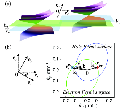
Figure 1: (a) 8-Pmmn borophene p-n junction. The normal (tangential) direction of the junction interface defines the $x^{\prime}$ ($y^{\prime}$) axis of the Cartesian coordinate system $x^{\prime}-y^{\prime}$. Along the energy axis, the Dirac point of N (P) region is at $-V_{0}$ ($V_{0}$) and the aligned Fermi level is at $E_{F}$. (b) Two Cartesian coordinate systems $x-y$ and $x^{\prime}-y^{\prime}$ are introduced and they are rotated to each other with $\theta$, so $\theta$ can be regarded as the junction direction. Using the coordinate systems, the electron (hole) Fermi surface in N (P) region is plotted. On the Fermi surfaces, we also plot the noncollinear momenta and group velocities of the incident, reflection, and transmission states. Here, we use $\theta=\pi/6$ for the junction direction, and $\varepsilon_{N}=\varepsilon_{P}=0.04$ eV for the doping levels in N and P regions.

The 8-Pmmn borophene PNJ structure is shown schematically by Fig. 1(a) and it has the left N region and right P region. For the PNJ, the Cartesian coordinate system $x^{\prime}-y^{\prime}$ is introduced, in which $x^{\prime}$ ($y^{\prime}$) axis is along the normal (tangential) direction of junction interface. The Hamiltonian of PNJ in Fig. 1(a) has the form:

$$\hat{H}=(\hat{H}_{0}-V_{0})\Theta(-x^{\prime})+(\hat{H}_{0}+V_{0})\Theta(x^{\prime}),$$ (1)

where $-V_{0}$ ($V_{0}$) is the gate-induced scalar potential in the N (P) region by assuming $V_{0}>0$ without loss of generality, and $\Theta(x^{\prime})$ is the step function: $\Theta(x^{\prime})=1$ for $x^{\prime}>0$ and $\Theta(x^{\prime})=0$ for $x^{\prime}<0$. The Fermi level $E_{F}$ determines the doping level in the N (P) region as $\varepsilon_{N}\equiv E_{F}+V_{0}$ ($\varepsilon_{P}\equiv E_{F}-V_{0}$), where a positive (negative) doping level means electron or N (hole or P) doping, so $\varepsilon_{N}>0$ and $\varepsilon_{P}<0$ in our case. For the intrinsic Hamiltonian $\hat{H}_{0}$ of 8-Pmmm borophene, we introduce the Cartesian coordinate system $x-y$ which is rotated in terms of $\theta$ relative to the coordinate system $x^{\prime}-y^{\prime}$ as shown in Fig. 1(b), so $\theta$ can be used to indicate the junction direction. The transformation relation between the basis vectors $(\mathbf{e}_{x},\mathbf{e}_{y})$ and $(\mathbf{e}_{x^{\prime}},\mathbf{e}_{y^{\prime}})$ of two coordinate systems is

$$\begin{bmatrix}\mathbf{e}_{x}\\ \mathbf{e}_{y}\end{bmatrix}=\left[\begin{array}[c]{cc}\cos\theta&-\sin\theta\\ \sin\theta&\cos\theta\end{array}\right]\begin{bmatrix}\mathbf{e}_{x^{\prime}}\\ \mathbf{e}_{y^{\prime}}\end{bmatrix}.$$ (2)

As a result, an arbitrary vector can be denoted by $\mathbf{O=(}O_{x},O_{y}\mathbf{)}$ in the coordinate system $x-y$ and by $\mathbf{O}^{\prime}\mathbf{=(}O_{x^{\prime}},O_{y^{\prime}}\mathbf{)}$ in the coordinate system $x^{\prime}-y^{\prime}$, and the vector’s components in two coordinate systems are related to each other:

$$O_{x} =O_{x^{\prime}}\cos\theta-O_{y^{\prime}}\sin\theta,$$ (3a)

$$O_{y} =O_{x^{\prime}}\sin\theta+O_{y^{\prime}}\cos\theta.$$ (3b)

Obviously, $$O=O^{\prime} O=\left|\mathbf{O}\right| O^{\prime}=\left|\mathbf{O}^{\prime}\right|$$ with and .

II.1 The intrinsic electronic properties of 8-Pmmn borophene

The Hamiltonian of anisotropic tilted MDF around one Dirac point of 8-Pmmn borophene is given byZabolotskiy and Lozovik (2016); Sadhukhan and Agarwal (2017); Islam and Jayannavar (2017)

$$\hat{H}_{0}=v_{x}\sigma_{x}\hat{p}_{x}+v_{y}\sigma_{x}\hat{p}_{y}+v_{t}\mathbf{I}_{2\times 2}\hat{p}_{y},$$ (4)

where $\hat{p}_{x,y}$ are the momentum operators, $\sigma_{x,y}$ are $2\times 2$ Pauli matrices, and $\mathbf{I}_{2\times 2}$ is the $2\times 2$ identity matrix. Throughout this paper, we assume $\hbar\equiv 1$. The anisotropic velocities are $v_{x}=0.86v_{F}$, $v_{y}=0.69v_{F}$, and $v_{t}=0.32v_{F}$ with $v_{F}=10^{6}$ m/s. The energy dispersion and the corresponding wave functions of $\hat{H}_{0}$ are, respectively,

$$E_{\lambda,\mathbf{k}}=v_{t}k_{y}+\lambda v_{x}\sqrt{k_{x}^{2}+\gamma_{1}^{2}k_{y}^{2}},$$ (5)

and

$$\psi_{\lambda,\mathbf{k}}(\mathbf{r})=\frac{1}{\sqrt{2}}\begin{bmatrix}1\\ \lambda\frac{\left(k_{x}+i\gamma_{1}k_{y}\right)}{\sqrt{k_{x}^{2}+\gamma_{1}^{2}k_{y}^{2}}}\end{bmatrix}e^{i\mathbf{k}\cdot\mathbf{r}}.$$ (6)

Here, $\gamma_{1}=v_{y}/v_{x}$, $\lambda=+$ ($\lambda=-$) denotes the conduction (valence) band, $\mathbf{k}=(k_{x},k_{y})$ is the momentum, and $\mathbf{r}=(x,y)$ is the position vector. The azimuthal angle of $\mathbf{k}$ relative to the $x$ axis is $\phi_{\mathbf{k}}$ which leads to tan$\phi_{\mathbf{k}}=k_{y}/k_{x}$, so the energy dispersion of Eq. (5) becomes

$$E_{\lambda,\mathbf{k}}=v_{t}k\sin\phi_{\mathbf{k}}+\lambda v_{x}k\sqrt{\cos^{2}\phi_{\mathbf{k}}+\gamma_{1}^{2}\sin^{2}\phi_{\mathbf{k}}}.$$ (7)

To determine the shape of Fermi surface for the fixing energy $E_{\lambda,\mathbf{k}}$, we can change Eq. (5) into

$$\frac{k_{x}^{2}}{k_{\lambda,a}^{2}}+\frac{(k_{y}+k_{\lambda,s})^{2}}{k_{\lambda,b}^{2}}=1,$$ (8)

where

$$k_{\lambda,s} =\frac{E_{\lambda,\mathbf{k}}v_{t}}{v_{y}^{2}-v_{t}^{2}},$$

$$k_{\lambda,a}^{2} =\frac{E_{\lambda,\mathbf{k}}^{2}v_{y}^{2}}{v_{x}^{2}(v_{y}^{2}-v_{t}^{2})},$$

$$k_{\lambda,b}^{2} =\frac{E_{\lambda,\mathbf{k}}^{2}v_{y}^{2}}{(v_{y}^{2}-v_{t}^{2})^{2}}.$$

Clearly, Eq. (8) is one equation of a shifted ellipse originated from the anisotropic tilted electronic properties. On one hand, the ratio of the semimajor and semiminor axes of the ellipse are $k_{\lambda,b}/k_{\lambda,a}=v_{x}/\sqrt{(v_{y}^{2}-v_{t}^{2})}\approx\sqrt{2}$ which does not depend on the energy dispersion $E_{\lambda,\mathbf{k}}$ (with the band index $\lambda$) and is a constant determined only by the anisotropic velocities. On the other hand, the ellipse is shifted along the $y$ axis such that its center lies at $(0,k_{\lambda,s})$. Because $k_{\lambda,s}\propto E_{\lambda,\mathbf{k}}$ and $E_{+,\mathbf{k}}\$and $E_{-,\mathbf{k}}$ have the opposite sign, the electron and hole Fermi surfaces are shifted oppositely along the $y$ axis. Combing these two features, the electron Fermi surface in the N region and the hole Fermi surface in the P region are shown in Fig. 1(b).

For convenience, we can define the pseudospin vector $\mathbf{s}=(s_{x},s_{y})$ for each state and

$$s_{x} \equiv\langle\psi_{\lambda,\mathbf{k}}|\sigma_{x}|\psi_{\lambda,\mathbf{k}}\rangle=\frac{\lambda k_{x}}{\sqrt{k_{x}^{2}+\gamma_{1}^{2}k_{y}^{2}}},$$ (9a)

$$s_{y} \equiv\langle\psi_{\lambda,\mathbf{k}}|\sigma_{y}|\psi_{\lambda,\mathbf{k}}\rangle=\frac{\lambda\gamma_{1}k_{y}}{\sqrt{k_{x}^{2}+\gamma_{1}^{2}k_{y}^{2}}}.$$ (9b)

So the azimuthal angle $$\phi_{\mathbf{s}} \mathbf{s}$$ of satisfies

$$\tan\phi_{\mathbf{s}}=s_{y}/s_{x}=\gamma_{1}\tan\phi_{\mathbf{k}}.$$ (10)

Then, Eq. 6(b) becomes

$$\psi_{\lambda,\mathbf{k}}(\mathbf{r})=\frac{1}{\sqrt{2}}\begin{bmatrix}1\\ e^{i\phi_{\mathbf{s}}}\end{bmatrix}e^{i\mathbf{k}\cdot\mathbf{r}}.$$ (11)

II.2 Transmission of anisotropic tilted MDF across PNJ

Firstly, because the translation invariance symmetry along the junction interface of PNJ requires the conservation of the tangential momentum $k_{y^{\prime}}$, it is convenient to derive the transmission probability of anisotropic tilted MDF across PNJ in the coordinate system $x^{\prime}-y^{\prime}$. Without loss of generality to consider the electron state incident from the left N region of PNJ, there are incident and reflection states in N region and transmission state in P region. In the following, we use

$$\psi^{\alpha}(\mathbf{r}^{\prime})=\frac{1}{\sqrt{2}}\begin{bmatrix}1\\ e^{i\phi_{\mathbf{s}}^{\alpha}}\end{bmatrix}e^{i\mathbf{k}_{\alpha}^{\prime}\cdot\mathbf{r}^{\prime}}$$ (12)

to denote the incident state $(\alpha=i)$, reflection state $(\alpha=r)$, and transmission state $(\alpha=t)$ in the mixed coordinate systems. Here, corresponding to the $\alpha$ state, $\phi_{\mathbf{s}}^{\alpha}$ is the azimuthal angle of pseudospin vector in the coordinate system $(x,y)$, and $\mathbf{k}_{\alpha}^{\prime}=(k_{\alpha,x}^{\prime},k_{y}^{\prime})$ is the momentum in the coordinate system $x^{\prime}-y^{\prime}$. Note that we use $k_{y}^{\prime}$ instead of $k_{\alpha,y}^{\prime}$ because $k_{y}^{\prime}$ is a conserved quantity. To solve the transmission problem, we obtain the matching equation for three states across the PNJ at $y^{\prime}=0$:

$$\psi^{i}(\mathbf{r}^{\prime})+r\psi^{r}(\mathbf{r}^{\prime})=t\psi^{t}(\mathbf{r}^{\prime}).$$ (13)

As a result, the reflection coefficient $r$ and transmission coefficient $t$ are:

$$r =-\frac{e^{i\phi_{\mathbf{s}}^{i}}-e^{i\phi_{\mathbf{s}}^{t}}}{e^{i\phi_{\mathbf{s}}^{r}}-e^{i\phi_{\mathbf{s}}^{t}}},$$ (14a)

$$t =1-r.$$ (14b)

The transmission probability of anisotropic tilted MDF across the PNJ is

$$T=1-|r|^{2},$$ (15)

whose calculation requires the value of $\mathbf{k}_{\alpha}=(k_{\alpha,x},k_{\alpha y})$ due to the Eqs. (9) and (10) for pseudospin vector in the coordinate system $(x,y)$. Note that $k_{\alpha y}$ is not conserved.

Secondly, we show how to obtain $\mathbf{k}_{r}$ and $\mathbf{k}_{t}$ for the calculation of $T$ by taking full advantage of the conserved $k_{y^{\prime}}$. The incident state has the momentum $\mathbf{k}_{i}=(k_{i,x},k_{i,y})=(k_{i}\cos\phi_{\mathbf{k}}^{i},k_{i}\sin\phi_{\mathbf{k}}^{i})$, which is one given quantity, and Eq. (7) implies

$$k_{i}=\frac{\varepsilon_{N}}{v_{t}\sin\phi_{\mathbf{k}}^{i}+v_{x}\sqrt{\cos^{2}\phi_{\mathbf{k}}^{i}+\gamma_{1}^{2}\sin^{2}\phi_{\mathbf{k}}^{i}}}.$$ (16)

This makes $\mathbf{k}_{i}^{\prime}=(k_{i,x^{\prime}},k_{y^{\prime}})=(k_{i}\cos\phi_{\mathbf{k}^{\prime}}^{i},k_{i}\sin\phi_{\mathbf{k}^{\prime}}^{i})$ with $\phi_{\mathbf{k}^{\prime}}^{i}=\phi_{\mathbf{k}}^{i}-\theta$ by considering Eq. (2) for transformation relation between two coordinate systems. Since $k_{y^{\prime}}=k_{i}\sin\phi_{\mathbf{k}^{\prime}}^{i}$ is obtained and conserved, in the following, we need to derive $k_{r,x^{\prime}}$ and $k_{t,x^{\prime}}$. By using Eq. (3), we obtain

$$k_{\alpha,x} =k_{\alpha,x^{\prime}}\cos\theta-k_{y^{\prime}}\sin\theta,$$ (17a)

$$k_{\alpha,y} =k_{\alpha,x^{\prime}}\sin\theta+k_{y^{\prime}}\cos\theta.$$ (17b)

Because $$\mathbf{k}_{\alpha}$$ satisfies Eq. (5) for energy dispersion, we obtain

$$Ak_{\beta,x^{\prime}}^{2}+B_{\beta}k_{\beta,x^{\prime}}+C_{\beta}=0,$$ (18)

where

$$A =\cos^{2}\theta+(\gamma_{1}^{2}-\gamma_{2}^{2})\sin^{2}\theta,$$

$$B_{\beta} =2\epsilon_{\beta}\gamma_{2}\sin\theta-2(1-\gamma_{1}^{2}+\gamma_{2}^{2})k_{y^{\prime}}\sin\theta\cos\theta,$$

$$C_{\beta} =k_{y^{\prime}}^{2}(\sin^{2}\theta+\gamma_{1}^{2}\cos^{2}\theta-\gamma_{2}^{2}\cos^{2}\theta)+2\epsilon_{\beta}\gamma_{2}k_{y^{\prime}}\cos\theta-\epsilon_{\beta}^{2}.$$

Here, $\gamma_{2}=v_{t}/v_{x}$, $\epsilon_{\beta}=\varepsilon_{\beta}/v_{x}$ with $\beta=N,P$. Equation (18) is a quadratic equation with one unknown and has two formal roots:

$$k_{\beta,x^{\prime}}^{\pm}=\frac{-B_{\beta}\pm\sqrt{B_{\beta}^{2}-4AC_{\beta}}}{2A}.$$

The right-going and left-going eigenstates should be finite when $x^{\prime}\rightarrow+\infty$ and $x^{\prime}\rightarrow-\infty$; this property can be used to distinguish them. In order to distinguish the left-going and right-going eigenstates, we make the replacement $E_{F}\rightarrow E_{F}+i0^{+}$ for the Fermi level in which $0^{+}$ is one positive infinitely small quantity. As a result, the right-going $k_{i,x^{\prime}}=k_{N,x^{\prime}}^{+}(=k_{i}\cos\phi_{\mathbf{k}^{\prime}}^{i})$ and $k_{t,x^{\prime}}=k_{P,x^{\prime}}^{+}$ both have the positive infinitely small imaginary part while the left-going $k_{r,x^{\prime}}=k_{N,x^{\prime}}^{-}$ has the negative infinitely small imaginary part. To substitute $k_{y^{\prime}}$ and derived $k_{r,x^{\prime}}$, $k_{t,x^{\prime}}$ into Eq. (17), one obtains $\mathbf{k}_{r,t}$, then can calculate the transmission probability $T$. For one given $\mathbf{k}_{i}$, we plot schematically $\mathbf{k}_{\alpha}$ on the electron and hole Fermi surfaces in Fig. 1(b).

III Results and discussions

In this section, we present the numerical results for the transmission probability of anisotropic tilted MDF across the borophene PNJ and discuss the underlying physics.

III.1 Existence of perfect transmission

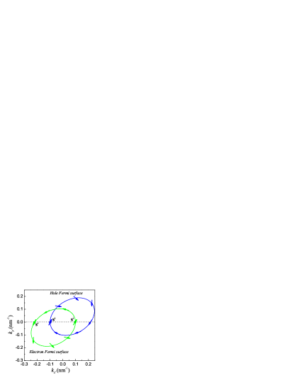
Figure 2: Pseudospin texture on the electron (hole) Fermi surface denoted by the green (blue) circle in the N (P) region. Perfect transmission occurs when $k_{y^{\prime}}=0$ (i.e., the black dotted line), meanwhile, the pseudospin orientation of the incident state is parallel to that of the transmission state and is antiparallel to that of the reflection state. Here, we use $\theta=\pi/3$ for the junction direction and $\varepsilon_{N}=\varepsilon_{P}=0.04$ eV for the doping levels in N and P regions.

Klein tunneling is one of the most exotic consequences of quantum electrodynamics, which was firstly discussed in condensed matter physics through investigating the tunneling properties of low-energy quasiparticles in graphene junctions Katsnelson et al. (2006). In graphene, the low-energy quasiparticles are isotropic MDF, which implies perfect transmission of MDF across PNJ at normal incidence. Klein tunneling is expected to occur in the borophene PNJ though its MDF are anisotropic and tilted. Previous to the numerical results, we analytically demonstrate the existence of perfect transmission in the borophene PNJ. From (Eq. 15), perfect transmission (i.e., $T=1$) occurs when $r=0$. $r$ is given by Eq. 14(a), $r=0$ leads to $e^{i\phi_{\mathbf{s}}^{i}}=e^{i\phi_{\mathbf{s}}^{t}}$ and $e^{i\phi_{\mathbf{s}}^{r}}\neq e^{i\phi_{\mathbf{s}}^{t}}$ which is just the well-known conservation of pseudospin $\mathbf{s}^{\alpha}$ Allain and Fuchs (2011), i.e., $\mathbf{s}^{i}\shortparallel\mathbf{s}^{t}$. Recalling that Klein tunneling occurs for the incident electron state with zero tangential momentum along the junction interface of graphene junctions Allain and Fuchs (2011), in the borophene PNJ, $k_{y^{\prime}}=0$ should be the necessary condition for the Klein tunneling. As shown in Fig. 1(b), the conserved $k_{y^{\prime}}$ determines the momentum positions of $\mathbf{k}_{t}$ ($\mathbf{k}_{i}$, $\mathbf{k}_{r}$) on the hole (electron) Fermi surface. When $k_{y^{\prime}}=0$, $\mathbf{k}_{i}$, $\mathbf{k}_{r}$, and $\mathbf{k}_{t}$ are collinear. Referring to Eqs. (9) and (10) for the pseudospin vector, we obtain $\phi_{\mathbf{s}}^{t}=\phi_{\mathbf{s}}^{i}$ and $\phi_{\mathbf{s}}^{r}=\phi_{\mathbf{s}}^{i}+\pi$, i.e., the pseudospin orientation of the incident state is parallel to that of the transmission state and is antiparallel to that of the reflection state as shown by Fig. 2, so perfect transmission exists for the incident anisotropic tilted MDF with $k_{y^{\prime}}=0$ or $\phi_{\mathbf{k}^{\prime}}^{i}=\theta$ in the borophene PNJ.

III.2 Noncollinear features of $\mathbf{v}_{\alpha}$ and $\mathbf{k}_{\alpha}$ induced by anisotropy and tilt

However, for a wave packet, the direction of center-of-mass motion and energy flow are described by the group velocity instead of the momentum Li et al. (2017). For isotropic MDF in graphene junctions, the group velocity and momentum of each state are collinear, so normal Klein tunneling is obtained. For the incident electronic state from the left N region of borophene PNJ, the group velocity $\mathbf{v}_{i}=(v_{i,x},v_{i,y})$ is determined by the energy dispersion of the conduction band (i.e., $\lambda=1)$ and

$$v_{i,x} \equiv\frac{\partial E_{+,\mathbf{k}_{i}}}{\partial k_{i,x}}=\frac{v_{x}k_{i,x}}{\sqrt{k_{i,x}^{2}+\gamma_{1}^{2}k_{i,y}^{2}}},$$ (19a)

$$v_{i,y} \equiv\frac{\partial E_{+,\mathbf{k}_{i}}}{\partial k_{i,y}}=v_{t}+\frac{v_{x}\gamma_{1}^{2}k_{i,y}}{\sqrt{k_{i,x}^{2}+\gamma_{1}^{2}k_{i,y}^{2}}},$$ (19b)

which leads to

$$\tan\phi_{{}_{\mathbf{V}}}^{i}=\gamma_{1}^{2}\tan\phi_{\mathbf{k}}^{i}+\gamma_{2}\sqrt{1+\gamma_{1}^{2}\tan^{2}\phi_{\mathbf{k}}^{i}}.$$ (20)

Here, $\phi_{{}_{\mathbf{V}}}^{i}$ is the azimuthal angle of $\mathbf{v}_{i}$. From Eq. (19), the anisotropy and tilt both lead to the noncollinear feature of the group velocity and the momentum. Similarly, one can define $\mathbf{v}_{r,t}$. In Fig. 1(b), we also plot $\mathbf{v}_{\alpha}$ to clearly show the noncollinear features of $\mathbf{v}_{\alpha}$ and $\mathbf{k}_{\alpha}$ which will bring about unique transmission properties in the borophene PNJ.

III.3 Oblique Klein tunneling

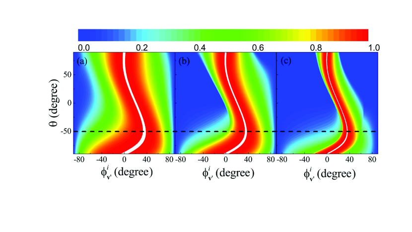
Figure 3: Contour plot for transmission probability as the function of the junction direction $\theta$ and the incident angle $\phi_{\mathbf{v}^{\prime}}^{i}=\phi_{\mathbf{v}}^{i}-\theta$ relative to the normal direction of borophene junction. (a) $E_{F}=-0.02$ eV, (b) $E_{F}=0$ eV, and (c) $E_{F}=0.02$ eV. In each panel, $V_{0}=0.04$ eV and the white color region with the transmission probability $T\geq 0.999$ is used to denote the parameter points for perfect transmission. The dashed black line denotes the special junction direction for the oblique Klein tunneling with the maximal difference between the perfect transmission direction and the normal direction of junction.

In the Cartesian coordinate system $x-y$, the electron and hole Fermi surfaces have the mirror symmetry about the $y$ axis as shown in Fig. 1(b), so the junction direction $\theta$ (i.e., the rotation angle between two coordinate systems) can be limited into the angle range $[-90^{\circ},90^{\circ}]$. Note that two cases for $\theta=90^{\circ}$ and $\theta=-90^{\circ}$ are not equivalent because of the different matching conditions for the incident, reflection, and transmission states. The group velocity of the incident state relative to the normal direction (i.e., $x^{\prime}$ axis) of borophene PNJ has the azimuthal angle $\phi_{\mathbf{v}^{\prime}}^{i}=\phi_{\mathbf{v}}^{i}-\theta$. Due to the isotropic nature of MDF in graphene junctions, perfect transmission occurs when $\phi_{\mathbf{v}^{\prime}}^{i}=0$. The case is very different in the borophene PNJ. As shown in Fig. 3, we present the contour plot for transmission probability of anisotropic tilted MDF as the function $\theta$ and $\phi_{\mathbf{v}^{\prime}}^{i}$ by considering different doping levels, i.e., (a) $E_{F}=-0.02$ eV, (b) $E_{F}=0$, and (c) $E_{F}=0.02$ eV when $V_{0}=0.04$ eV. Figure 3 shows several interesting properties. (1) As changing junction direction of borophene PNJ by tuning $\theta$, perfect transmission must occur consistent with the analytical demonstration in Sec. IIIA. (2) The direction for perfect transmission deviates the normal direction of borophene PNJ, i.e., $\phi_{\mathbf{v}^{\prime}}^{i}\neq 0$. For convenience, this phenomenon is named as oblique Klein tunneling, which is in sharp contrast to the normal Klein tunneling in the graphene PNJ. (3) By comparing the perfect transmission in three subfigures, we find that the departure of oblique Klein tunneling from the normal direction of borophene PNJ does not depend on the doping level. The behavior can be understood in terms of Eq. (20) in which$\ \phi_{\mathbf{k}}^{i}=\theta$ for perfect transmission as discussed in Sec. IIIA. As a result, the difference between the perfect transmission direction and the normal direction only depends on $\theta$. Furthermore, the special $\theta_{m}$ gives the maximal difference between the two directions. To obtain the $\theta_{m}$ for oblique Klein tunneling, we need to maximize $(\theta-\phi_{\mathbf{v}})$ or equivalently $\tan(\theta-\phi_{\mathbf{v}})$. Using Eq. (20), we obtain

$$\tan(\theta-\phi_{\mathbf{v}})=\frac{1-\gamma_{1}^{2}}{\gamma_{2}}\cos\tilde{\theta}-\frac{1+\gamma_{2}^{2}-\gamma_{1}^{2}}{\gamma_{2}}\frac{\cos\tilde{\theta}}{1+\gamma\sin\tilde{\theta}},$$ (21)

where $\gamma=\gamma_{2}/\gamma_{1}$ and

$$\tan\tilde{\theta}=\gamma_{1}\tan\theta.$$ (22)

The extrema of $\tan(\theta-\phi_{\mathbf{v}})$ is determined by

$$\frac{\partial\tan(\theta-\phi_{\mathbf{v}})}{\partial\tilde{\theta}}=0,$$

which gives

$$az^{3}+bz^{2}+cz+d=0.$$ (23)

Here, $z=\sin\tilde{\theta}$, $a=\gamma^{2}$, $b=2\gamma$, $c=1-c_{1}/c_{2}$ , and $d=-\gamma c_{1}/c_{2}$ with $c_{1}=(1+\gamma_{2}^{2}-\gamma_{1}^{2})/\gamma_{2}$ and $c_{2}=(1-\gamma_{1}^{2})/\gamma_{2}$. Equation (23) is one cubic equation, and its general solutions are

$$z_{n}=-\frac{1}{3a}(b+\xi^{n}C+\frac{\Delta_{0}}{\xi^{n}C}),n\in\{0,1,2\},$$

with

$$\xi=-\frac{1}{2}+\frac{\sqrt{3}}{2}i$$

and

$$\Delta =18abcd-4b^{3}d+b^{2}c^{2}-4ac^{3}-27a^{2}d^{2},$$

$$\Delta_{0} =b^{2}-3ac,$$

$$\Delta_{1} =2b^{3}-9abc+27a^{2}d,$$

$$C =\sqrt[3]{\frac{\Delta_{1}\pm\sqrt{-27a^{2}\Delta}}{2}}.$$

Because $\Delta\simeq 2.617>0$, the cubic equation has three real roots and they are

$$z_{0} \approx-4.565,$$

$$z_{1} \approx-0.694,$$

$$z_{2} \approx 0.946.$$

Recalling $\left|z\right|\leq 1$ due to $z=\sin\tilde{\theta}$, so $z_{1,2}$ are the two proper roots. Equation (22) gives

$$\theta=\arctan(\frac{\gamma_{1}z}{\sqrt{1-z^{2}}}).$$ (24)

Substituting $z_{1,2}$ into the above Eq. (24), we obtain

$$\theta_{1} =-0.877\text{ rad}=-50.228^{\circ},$$

$$\theta_{2} =1.302\text{ rad}=74.627^{\circ}.$$

For the difference between the perfect transmission direction and the normal direction, $\theta_{1}$ ($\theta_{2}$) gives the global maximum (local minimum) as shown by Fig. 3, so

$$\theta_{m}=\theta_{1}=-50.228^{\circ}$$ (25)

which is denoted by the black dashed line and is independent on doping level. At $\theta_{m}$, it is $35.\,\allowbreak 838^{\circ}$ for the maximal difference between the perfect transmission direction and the normal direction. The anisotropy and tilt of MDF in borophene PNJ both contribute to $\theta_{m}$. If no tilt ($v_{t}=0$), $\theta_{m}$ contributed by the anisotropy is $\theta_{m}^{a}=\arctan(1/\gamma_{1})=51.\,\allowbreak 259^{\circ}$. The drastic difference between $\theta_{m}^{a}$ and $\theta_{m}$ implies that the tilt plays an important role leading to the oblique Klein tunneling. Therefore, the unique features of oblique Klein tunneling are intimately related to the nature of MDF, so they can be used to identify the anisotropy and/or tilt of energy dispersion.

IV Conclusions and outlook

In this study, we investigate analytically the transport properties of anisotropic and tilted MDF in the 8-Pmmn borophene PNJ. The unique oblique Klein tunneling induced by the anisotropy and tilt of MDF is shown, which does not depend on the doping levels in N and P regions of PNJ as the normal Klein tunneling. To obtain the maximal difference between perfect transmission direction and the normal direction of PNJ, we analytically determine the junction direction. In addition, the respective contribution of anisotropy and tilt underlying the oblique Klein tunneling is also distinguished, this makes the transmission measurement be useful to reveal the character of the energy dispersion.

In order to analytically show the oblique Klein tunneling of anisotropic and tilted MDF, two simplifications for the realistic 8-Pmmn borophene PNJ has been used, i.e., the single Dirac cone and the sharp junction are considered. The 8-Pmmn borophene has two inequivalent Dirac cones described by low-energy effective Hamiltonian $\hat{H}_{\eta}=\eta\hat{H}_{0}$ with $\eta=\pm$ denoting two cones Zabolotskiy and Lozovik (2016); Sadhukhan and Agarwal (2017); Islam and Jayannavar (2017). If neglecting the intervalley scattering, referring to the detailed presentations for the $\eta=+$ cone, one can easily derive the results corresponding to $\eta=-$ cone, e.g., the valley-dependent special junction direction $\theta_{m}^{\eta}=\eta\theta_{m}$ which may favor the application of 8-Pmmn borophene in valleytronics. The effect of intervalley scattering depends on the width and direction of PNJ Logemann et al. (2015). For the junction width beyond the atomically scale, the intervalley scattering can be neglected properly due to the large momentum difference between two Dirac cones Katsnelson (2012). However, the simplification of sharp junction implies that the electron wavelength should be larger than junction width, otherwise a too broad junction will impede the transmission of oblique electron states across the PNJ Cheianov and Fal’ko (2006) and is harmful to the application of PNJ in electron optics Chen et al. (2016). Therefore, our analytical results are applicable to the low-energy electrons scattered by PNJ with a rather smooth junction and should be mainly used to understand the novel physical features accompanying the anisotropic and tilted MDF in contrast to those of isotropic MDF (e.g., in graphene Katsnelson (2012)). In light of the experimental advances for confirming different borophene monolayers Mannix et al. (2015); Feng et al. (2016, 2017), for fabricating sharp junctions on the nanoscale Bai et al. (2018), and for demonstrating the prominent angular dependence of the transmission probability in planar PNJ structures Sajjad et al. (2012); Sutar et al. (2012); Rahman et al. (2015); Chen et al. (2016), we expect the oblique Klein tunneling to be observable in the near future. In order to compare to future experiments, the further quantitative atomic simulation is needed by using a proper numerical method Zhang et al. (2017b).

References

- Castro Neto et al. (2009) A. H. Castro Neto, F. Guinea, N. M. R. Peres, K. S. Novoselov, and A. K. Geim, Rev. Mod. Phys. 81, 109 (2009).
- Wehling et al. (2014) T. Wehling, A. Black-Schaffer, and A. Balatsky, Advances in Physics 63, 1 (2014).
- Wang et al. (2015) J. Wang, S. Deng, Z. Liu, and Z. Liu, National Science Review 2, 22 (2015).
- Zhang et al. (2017a) Z. Zhang, E. S. Penev, and B. I. Yakobson, Chem. Soc. Rev. 46, 6746 (2017a).
- Kondo (2017) T. Kondo, Science and Technology of Advanced Materials 18, 780 (2017).
- Zhou et al. (2014) X.-F. Zhou, X. Dong, A. R. Oganov, Q. Zhu, Y. Tian, and H.-T. Wang, Phys. Rev. Lett. 112, 085502 (2014).
- Lopez-Bezanilla and Littlewood (2016) A. Lopez-Bezanilla and P. B. Littlewood, Phys. Rev. B 93, 241405 (2016).
- Zabolotskiy and Lozovik (2016) A. D. Zabolotskiy and Y. E. Lozovik, Phys. Rev. B 94, 165403 (2016).
- Nakhaee et al. (2018) M. Nakhaee, S. A. Ketabi, and F. M. Peeters, Phys. Rev. B 97, 125424 (2018).
- Pereira and Castro Neto (2009) V. M. Pereira and A. H. Castro Neto, Phys. Rev. Lett. 103, 046801 (2009).
- Naumis et al. (2017) G. G. Naumis, S. Barraza-Lopez, M. Oliva-Leyva, and H. Terrones, Reports on Progress in Physics 80, 096501 (2017).
- Sadhukhan and Agarwal (2017) K. Sadhukhan and A. Agarwal, Phys. Rev. B 96, 035410 (2017).
- Verma et al. (2017) S. Verma, A. Mawrie, and T. K. Ghosh, Phys. Rev. B 96, 155418 (2017).
- Islam and Jayannavar (2017) S. F. Islam and A. M. Jayannavar, Phys. Rev. B 96, 235405 (2017).
- Mannix et al. (2015) A. J. Mannix, X.-F. Zhou, B. Kiraly, J. D. Wood, D. Alducin, B. D. Myers, X. Liu, B. L. Fisher, U. Santiago, J. R. Guest, et al., Science 350, 1513 (2015).
- Feng et al. (2016) B. Feng, J. Zhang, Q. Zhong, W. Li, S. Li, H. Li, P. Cheng, S. Meng, L. Chen, and K. Wu, Nature Chemistry 8, 563 (2016).
- Feng et al. (2017) B. Feng, O. Sugino, R.-Y. Liu, J. Zhang, R. Yukawa, M. Kawamura, T. Iimori, H. Kim, Y. Hasegawa, H. Li, et al., Phys. Rev. Lett. 118, 096401 (2017).
- Cheng et al. (2017) T. Cheng, H. Lang, Z. Li, Z. Liu, and Z. Liu, Phys. Chem. Chem. Phys. 19, 23942 (2017).
- Klein (1929) O. Klein, Z. Phys. 53, 157 (1929).
- Katsnelson et al. (2006) M. I. Katsnelson, K. S. Novoselov, and A. K. Geim, Nat. Phys. 2, 620 (2006).
- Cheianov and Fal’ko (2006) V. V. Cheianov and V. I. Fal’ko, Phys. Rev. B 74, 041403 (2006).
- Pereira et al. (2006) J. M. Pereira, V. Mlinar, F. M. Peeters, and P. Vasilopoulos, Phys. Rev. B 74, 045424 (2006).
- Bai and Zhang (2007) C. Bai and X. Zhang, Phys. Rev. B 76, 075430 (2007).
- Beenakker et al. (2008) C. W. J. Beenakker, A. R. Akhmerov, P. Recher, and J. Tworzydło, Phys. Rev. B 77, 075409 (2008).
- Setare and Jahani (2010) M. R. Setare and D. Jahani, J. Phys. Condens. Matter 22, 245503 (2010).
- Roslyak et al. (2010) O. Roslyak, A. Iurov, G. Gumbs, and D. Huang, J. Phys. Condens. Matter 22, 165301 (2010).
- Zeb et al. (2008) M. A. Zeb, K. Sabeeh, and M. Tahir, Phys. Rev. B 78, 165420 (2008).
- Sonin (2009) E. B. Sonin, Phys. Rev. B 79, 195438 (2009).
- Schelter et al. (2010) J. Schelter, D. Bohr, and B. Trauzettel, Phys. Rev. B 81, 195441 (2010).
- Yang et al. (2011) R. Yang, L. Huang, Y.-C. Lai, and C. Grebogi, Phys. Rev. B 84, 035426 (2011).
- Rozhkov et al. (2011) A. Rozhkov, G. Giavaras, Y. P. Bliokh, V. Freilikher, and F. Nori, Phys. Rep. 503, 77 (2011).
- Liu et al. (2012) M.-H. Liu, J. Bundesmann, and K. Richter, Phys. Rev. B 85, 085406 (2012).
- Giavaras and Nori (2012) G. Giavaras and F. Nori, Phys. Rev. B 85, 165446 (2012).
- Rodriguez-Vargas et al. (2012) I. Rodriguez-Vargas, J. Madrigal-Melchor, and O. Oubram, J. Appl. Phys. 112, 073711 (2012).
- Popovici et al. (2012) C. Popovici, O. Oliveira, W. de Paula, and T. Frederico, Phys. Rev. B 85, 235424 (2012).
- Heinisch et al. (2013) R. L. Heinisch, F. X. Bronold, and H. Fehske, Phys. Rev. B 87, 155409 (2013).
- Logemann et al. (2015) R. Logemann, K. J. A. Reijnders, T. Tudorovskiy, M. I. Katsnelson, and S. Yuan, Phys. Rev. B 91, 045420 (2015).
- Bai et al. (2016) C. Bai, Y. Yang, and K. Chang, Scientific Reports 6, 21283 (2016).
- Oh et al. (2016) H. Oh, S. Coh, Y.-W. Son, and M. L. Cohen, Phys. Rev. Lett. 117, 016804 (2016).
- Erementchouk et al. (2016) M. Erementchouk, P. Mazumder, M. A. Khan, and M. N. Leuenberger, J. Phys. Condens. Matter 28, 115501 (2016).
- Downing and Portnoi (2017) C. A. Downing and M. E. Portnoi, J. Phys. Condens. Matter 29, 315301 (2017).
- Zhang and Yang (2018) S.-H. Zhang and W. Yang, Phys. Rev. B 97, 035420 (2018).
- Huard et al. (2007) B. Huard, J. A. Sulpizio, N. Stander, K. Todd, B. Yang, and D. Goldhaber-Gordon, Phys. Rev. Lett. 98, 236803 (2007).
- Gorbachev et al. (2008) R. V. Gorbachev, A. S. Mayorov, A. K. Savchenko, D. W. Horsell, and F. Guinea, Nano Lett. 8, 1995 (2008).
- Stander et al. (2009) N. Stander, B. Huard, and D. Goldhaber-Gordon, Phys. Rev. Lett. 102, 026807 (2009).
- Young and Kim (2009) A. F. Young and P. Kim, Nat. Phys. 5, 222 (2009).
- Rossi et al. (2010) E. Rossi, J. H. Bardarson, P. W. Brouwer, and S. Das Sarma, Phys. Rev. B 81, 121408 (2010).
- Sajjad et al. (2012) R. N. Sajjad, S. Sutar, J. U. Lee, and A. W. Ghosh, Phys. Rev. B 86, 155412 (2012).
- Sutar et al. (2012) S. Sutar, E. S. Comfort, J. Liu, T. Taniguchi, K. Watanabe, and J. U. Lee, Nano Lett. 12, 4460 (2012).
- Rahman et al. (2015) A. Rahman, J. W. Guikema, N. M. Hassan, and N. Marković, Appl. Phys. Lett. 106, 013112 (2015).
- Guti rrez et al. (2016) C. Guti rrez, L. Brown, C. J. Kim, J. Park, and A. N. Pasupathy, Nat. Phys. 12, 1069 (2016).
- Chen et al. (2016) S. Chen, Z. Han, M. M. Elahi, K. M. M. Habib, L. Wang, B. Wen, Y. Gao, T. Taniguchi, K. Watanabe, J. Hone, et al., Science 353, 1522 (2016).
- Laitinen et al. (2016) A. Laitinen, G. S. Paraoanu, M. Oksanen, M. F. Craciun, S. Russo, E. Sonin, and P. Hakonen, Phys. Rev. B 93, 115413 (2016).
- Bai et al. (2017) K.-K. Bai, J.-B. Qiao, H. Jiang, H. Liu, and L. He, Phys. Rev. B 95, 201406 (2017).
- Sajjad and Ghosh (2011) R. N. Sajjad and A. W. Ghosh, Appl. Phys. Lett. 99, 123101 (2011).
- Jang et al. (2013) M. S. Jang, H. Kim, Y.-W. Son, H. A. Atwater, and W. A. Goddard, Proc. Natl. Acad. Sci. 110, 8786 (2013).
- Wilmart et al. (2014) Q. Wilmart, S. Berrada, D. Torrin, V. H. Nguyen, G. Fève, J.-M. Berroir, P. Dollfus, and B. Plaçais, 2D Materials 1, 011006 (2014).
- Chen and Chang (2015) C.-C. Chen and Y.-C. Chang, Phys. Rev. B 92, 245406 (2015).
- de Sousa et al. (2017) D. J. P. de Sousa, A. Chaves, J. M. PereiraJr., and G. A. Farias, J. Appl. Phys. 121, 024302 (2017).
- Li et al. (2017) Z. Li, T. Cao, M. Wu, and S. G. Louie, Nano Letters 17, 2280 (2017).
- Nguyen and Charlier (2018) V. H. Nguyen and J.-C. Charlier, Phys. Rev. B 97, 235113 (2018).
- Allain and Fuchs (2011) P. E. Allain and J. Fuchs, The European Physical Journal B 83, 301 (2011).
- Katsnelson (2012) M. I. Katsnelson, Graphene: Carbon in Two Dimensions (Cambridge University Press, New York, 2012).
- Bai et al. (2018) K.-K. Bai, J.-J. Zhou, Y.-C. Wei, J.-B. Qiao, Y.-W. Liu, H.-W. Liu, H. Jiang, and L. He, Phys. Rev. B 97, 045413 (2018).
- Zhang et al. (2017b) S.-H. Zhang, W. Yang, and K. Chang, Phys. Rev. B 95, 075421 (2017b).