A Multi-View Ensemble Classification Model for Clinically Actionable Genetic Mutations

Abstract

This paper presents details of our winning solutions to the task IV of NIPS 2017 Competition Track entitled Classifying Clinically Actionable Genetic Mutations. The machine learning task aims to classify genetic mutations based on text evidence from clinical literature with promising performance. We develop a novel multi-view machine learning framework with ensemble classification models to solve the problem. During the Challenge, feature combinations derived from three views including document view, entity text view, and entity name view, which complements each other, are comprehensively explored. As the final solution, we submitted an ensemble of nine basic gradient boosting models which shows the best performance in the evaluation. The approach scores $0.5506$ and $0.6694$ in terms of logarithmic loss on a fixed split in stage-$1$ testing phase and $5$-fold cross validation respectively, which also makes us ranked as a top-$1$ team out of more than $1300$ solutions in NIPS $2017$ Competition Track IV.

1 Introduction

The NIPS $2017$ Competition Track IV arises from gene mutation classification using Natural Language Processing (NLP). Gene mutation classification, which is one of the important problems in Precision Medicine, aims at distinguishing the mutations that contribute to tumor growth (drivers) from the neutral mutations (passengers). Identifying types of gene mutations is helpful in determining emerging molecular tumors and finding drugs that can treat them Tutorials . In order to classify clinically actionable genetic mutations, the related biomedical scholarly articles are a trustworthy knowledge source. Currently, this interpretation of genetic mutations is being done manually. This is a quite time-consuming task where a clinical pathologist has to manually review and classify every single genetic mutation based on evidence from articles.

The Competition Track releases a dataset of oncogenes he2005microrna , along with their corresponding mutations and related articles obtained from PubMed, an online biomedical literature repository. The goal is to design machine learning approaches which can predict class labels for gene mutation samples with acceptable accuracy. The target classes have been predefined by the Challenge organizer Memorial Sloan Kettering Cancer Center (MSKCC). Specifically, they are “Gain-of-function”, “Likely Gain-of-function”, “Loss-of-function”, “Likely Loss-of-function”, “Neutral”, “Likely Neutral”, “Switch-of-function”, “Likely Switch-of-function”, and “Inconclusive”. Therefore, it is a multi-class classification task.

Basically, the competition can be viewed as a text classification task based on clinical descriptions of gene mutations. However, the problem is more challenging than traditional document classification problem that is handled with NLP benchmarks in many aspects. Our useful observations about the difficulties are summarized as follows:

• Different samples may share the same text entry, while their class labels are entirely different. From the statistics shown in Fig. 1, there are a bunch of cases in which various samples share the same text. Instead of mining knowledge from original documents, more evidence from other perspective is necessary.

• Each sample is associated with an extremely long document with a large amount of noisy information that makes the problem difficult. As the word count distribution shown in Fig. 2, documents generally contain much more sentences than the normal text classification datasets textclassification .

• While a gene and its corresponding label distribution over classes could be a great hint in the prediction, the fact that there are only a few overlapped samples in training and testing set makes the distributional information useless. Basically, we can only summarize effective features from characters through entity names.

Figure 1: Distribution of the counts of common text that are shared by different samples. The head of the distribution is shown here. When we give all the observed text a unique id, the most common text is used more than 50 times by gene mutation samples.

Figure 2: Distribution of the text entry lengths. The median value of word count per text is 6,743 while the maximum word count in a text is 77,202.

In order to deal with above challenges, a multi-view ensemble classification framework is proposed. Concretely, we extract prior knowledge about genes and mutations globally from the sentences mentioning the specific genes or mutations in the text collection. Hence, we are able to design text features not only for the original document view but also for the entity (gene/mutation) text view to address the first two difficulties above-mentioned. To make full use of the entity name information, the third view for names is also explored using word embedding or character-level n-gram encoding. Furthermore, we combine features derived from three views to implement basic classification models and exploit features from each view complements to each other. After that, we ensemble the basic models together by several strategies to boost the final accuracy. The data and source code are available at https://github.com/sheryl-ai/NeurIPS17.

The rest of the paper is organized as follows. Section 2 introduces main notations, the validation dataset, and the evaluation metric. In Section 3, the multi-view text mining approach is explained. Model ensemble methods are presented in Section 4. Empirical study and analysis are provided in Section 5. Eventually, several conclusions are given in Section 6.

2 Preliminary

2.1 Notations

Table 1: main notations used in this paper

Symbols	Definition
$\mathbf{x}$	feature vector
$\mathbf{x}^{D}$	feature vector in original document view
$\mathbf{x}^{ET}$	feature vector in entity text view
$\mathbf{x}^{ET}_{g}$	gene feature vector in entity text view
$\mathbf{x}^{ET}_{m}$	mutation feature vector in entity text view
$\mathbf{x}^{EN}$	feature vector in entity name view
$\mathbf{x}^{EN}_{g}$	gene feature vector in entity name view
$\mathbf{x}^{EN}_{m}$	mutation feature vector in entity name view
$N$	the number of samples
$M$	the number of classes
$y_{ij}$	binary indicator whether label $j$ is true for sample $i$
$p_{ij}$	predicted probability of assigning label $j$ to sample $i$
$\mathcal{T}^{r}$	training set
$\mathcal{T}^{v}$	validation set
$\mathcal{T}^{s}$	testing set
$\hat{p}^{v}_{ij}$	predicted probability for validation set data
$\hat{p}^{s}_{ij}$	predicted probability for testing set data
$\alpha$	linear combination parameter for basic models

Table 1 lists some main notations used throughout the paper. In the paper, genes, mutations, and their corresponding documents are respectively denoted by $g$, $m$, and $d$. Each sample is constructed by a triplet $<gene,mutation,document>$. The feature vector generated for each sample is denoted as the vector $\mathbf{x}$. Feature vectors in the three views are represented as $\mathbf{x}^{D}$, $\mathbf{x}^{ET}$, and $\mathbf{x}^{EN}$ respectively. With notations presented in Table 1, our problem can be explicitly defined as:

Definition

Given sample sets $\{<g_{i},m_{i},d_{i}>\}_{i=1}^{N}$, our aim is to generate feature vectors $\{\mathbf{x}_{i}^{D},\mathbf{x}_{i}^{ET},\mathbf{x}_{i}^{EN}\}_{i=1}^{N}$ in multiple views, so that probabilities of label assignment over $M$ possible class can be predicted.

2.2 Validation Set

Table 2: Statistics of the stage-$1$ datasets

	training	validation
# of samples	3,321	368
# of unique genes	264	140
# of unique mutations	2,996	328

The Challenge consists of two stages and released a training set and a validation set in stage-$1$. During stage-$1$, the labels of the validation set are unknown and participants can verify the performances of their models online by submitting the classification results of the validation set. The stage-$1$ of this Challenge lasted for a couple of weeks, while the ongoing stage-$2$ was held in the final week. In stage-$2$, the stage-$1$ training data, validation data, and new online test data without labels are given. The stage-$1$ training set contains $3,321$ gene mutation samples with $264$ unique genes and $2,996$ unique mutations. The validation set contains $368$ gene mutation samples with $140$ unique genes and $328$ unique mutations. In total, we have $3,689$ training samples including $269$ unique genes and $3,309$ unique mutations. The detailed data statistics for the training set and the validation set can be found in Table 2.

The stage-$1$ validation data is used to generate the rankings on the Leaderboard of the first stage. On the one hand, we perform offline validation without submitting classification results using the validation set. On the other hand, it can be used to extend the size of training set during the second stage of this competition. In this work, we denote the stage-$1$ training set ($3,321$ samples) by $\mathcal{T}^{r}$, and denote the stage-$1$ validation set ($368$ samples) by $\mathcal{T}^{v}$. The online testing set of stage-$2$ for submission is denoted by $\mathcal{T}^{s}$.

2.3 Evaluation Metric

The Challenge adopts logarithmic loss as the evaluation metric. It measures performance of a multi-class classification model where the prediction is a probability distribution over classes between $0$ and $1$. Mathematically, the Logloss is defined as:

$$-\frac{1}{N}\Sigma_{i=1}^{N}\Sigma_{j=1}^{M}y_{ij}log(p_{ij})$$ (1)

where $N$ and $M$ are the number of samples and the number of the possible class label, respectively. $y_{ij}$ is a binary indicator of whether or not label $j$ is the correct classification for sample $i$, and $p_{ij}$ is the output probability of assigning label $j$ to instance $i$. By minimizing log loss, the accuracy of the classifier is maximized. In other words, a smaller value of the metric indicates a more accurate classifier.

3 The Proposed Approach

Given the gene mutations and their associated articles, a straightforward approach is to extract features directly from the documents and entity names. As we introduced, this approach might suffer the fact that two samples share same text but have different class labels. Considering a gene BRCA1, it owns two possible mutations: T1773I and M1663L in two different samples, with their gene mutation types are “Likely Loss-of-function” and “Likely Neutral”, respectively. The article descriptions, however, are exactly same for the two samples. The straightforward document classification approach cannot work well in this case, since it is fairly difficult for the classifier to categorize the samples into correct classes only via the name of mutations (normally a few characters construct the names).

Figure 3: The classification framework (best viewed in color). Four data files are released by the Challenge: training/testing variants and training/testing text. The three colored arrows from data files to feature mining modules indicate three aspects of feature engineering. Document features are only derived from text data; entity text features need both variants and text; entity name features derive from variants as well as text data (Word embedding model is also trained using the given text).

Fig. 3 presents an overview of our multi-view framework for solving this problem. The original input data includes training and testing variants (the name information of gene mutations), training and testing texts (the associated articles). In our solution, we perform feature extraction and engineering from the following three views:

• Document view: original documents associated with gene mutation samples (denoted by blue arrows in Fig. 3);

• Entity text view: sentences globally extracted from the document collection associated with genes and mutations (denoted by green arrows in Fig. 3);

• Entity name view: characters of the gene names and mutation names (denoted by purple arrows in Fig. 3).

After feature engineering, we first concatenate the gene text feature with mutation text feature to represent each sample. In particular, $\mathbf{x}_{g}^{ET}$ and $\mathbf{x}_{m}^{ET}$ are concatenated to form the feature vector of entity text $\mathbf{x}^{ET}=\mathbf{x}_{g}^{ET}\|\mathbf{x}_{m}^{ET}$, where $\|$ denotes concatenation operation. Similarly, the feature vector of entity name is formed by concatenation $\mathbf{x}^{EN}=\mathbf{x}_{g}^{EN}\|\mathbf{x}_{m}^{EN}$. Then features from three views are combined to train multiple classification models and generate multiple prediction results. Various combination schemes are explored to decide the feature sets with the best accuracy (see Section 4). The feature generation and combination will be introduced in the following sections.

3.1 Document View

Domain Knowledge

Domain knowledge usually provides extra pieces of information for classification task. To incorporate biomedical domain knowledge, feature dimensions including bioentities and keywords are extracted.

Genes and mutations may have alias in PubMed articles. Also, quite a lot bioentities appear in the text but not be included in samples. A proper utilization of the bioentity information is an important part of a successful solution. Thanks to a Named Entity Recognition (NER) tool PubTator wei2013pubtator , we can extract the entity dictionary for the entities in the text data. The PubTator is used to enrich the dictionaries of genes and mutations using the abstracts of the related PubMed articles. The tool includes GeneTUKit huang2011genetukit , GenNorm gennorm and tmVar wei2013tmvar . Finally, we obtain bioentities containing $2,668$ chemicals, $2,486$ diseases, $6,987$ genes, and $2,486$ mutations.

In addition to the document corpus provided by this Challenge, we also built a dictionary by Keywords extracted from related PubMed articles obtained from OncoKB. The underlying assumption is that the keywords detected from titles of the related articles are the essential terms in the research domain. In particular, the keywords are extracted from the titles of those articles by removing the stop words and punctuations. The keywords dictionary has $3,379$ unique words.

Document-Level Feature

While traditional feature engineering will always be staples of machine learning pipelines, representation learning has emerged as an alternative approach to feature extraction. In order to represent a document by natural language modeling, paragraph vectors or Doc2Vec doc2vec is exploited. Doc2Vec can be viewed as a generalization of Word2Vec Word2Vec approach. In addition to considering context words, it considers the specific document when predicting a target word, and thus it can exploit the word ordering along with their semantic relationships. With a trained Doc2Vec model, we can get a vector representation with a fixed length for any given document with arbitrary lengths.

Doc2Vec provides two training strategies to model the context in documents, which are distributed memory model (PV-DM) and distributed bag-of-word model (PV-DBOW). PV denotes paragraph vector here. Given sequences of training words in paragraphs, the PV-DM model is trained to get paragraph vectors, word vectors, softmax weights and bias to maximize the probability of seen texts. The difference between the two versions are: PV-DM simultaneously uses the context words and a paragraph matrix to predict the next word while PV-DBOW ignores the context words in the input but uses the parameter matrix to predict words randomly sampled from the paragraphs, which leads to less storage. As recommended in doc2vec , we combine the outputs of PV-DM with PV-DBOW together to achieve the best performance (concatenation of $150$ dimensions for PV-DM and $250$ dimensions for PV-DBOW).

Sentence-Level Feature

When it comes to extracting features from very noisy long documents, filtering sentences might be a choice to obtain effective knowledge. Regarding sentences mentioning the genes or mutations as key sentences, the context of key sentences is also used to capture the useful information. The basic assumption behind is that words in the same context tend to have similar meanings. For the reason that the articles have sufficient sentences to satisfy the distributional hypothesis theory harris , we extend the concept ”word” to ”sentence” to form contexts. Considering a key sentence $s_{t}$ and its Term Frequency-Inverse Document Frequency (TF-IDF) feature vector $\mathbf{x}_{s,t}$, the context can be represented as concatenation: $\mathbf{x}_{s,t-1}\|\mathbf{x}_{s,t}\|\mathbf{x}_{s,t+1}$ when the window size is set as $3$. Then the representation for documents in samples can be calculated by averaging the key contexts. Here we adopt average values and call the defined feature as sentence-level TF-IDF.

Word-Level Feature

Nouns, verbs, adjectives, and adverbs are four major word types we considered in Part-of-Speech (PoS) Tagging postagging ; wordnet . In the scenario of genetic mutation classification, nouns could be the names of proteins, diseases, drugs, and so on, which serve as important clues for predicting mutation classes. The verb type includes most of the words referring to actions and processes such as interact, affect, and detect. In addition, adjectives are considered since they reflect properties of nouns while adverbs might semantically reflect some discoveries or conclusions like dramatically, or consistently. Our method takes all of the word tokens as input with preprocessing steps including filtering out stop words and punctuations, stemming and lemmatization, and PoS tagging. Then a dictionary with $9,868$ words of all the four types is constructed.

TF-IDF is one of the common used measures that computes the importance of each word in a document tfidf . Given a collection of $N$ documents. TF-IDF assigns to term $t$ a weight in document $d$ given by $\mathrm{tfidf}_{td}=\mathrm{tf}_{td}\times\mathrm{idf}_{t}$, where inverse document frequency can be defined as $\mathrm{idf}_{t}=log\frac{N}{\mathrm{df}_{t}}$. Document frequency $\mathrm{df}_{t}$ means the number of documents in the collection that contain term $t$. Our new strategy is to embed the discriminative power of each term. Intuitively the $\mathrm{idf}_{t}$ should be calculated by class frequency, that is, $\mathrm{idf}_{t}=log\frac{M}{\mathrm{cf}_{t}}$, where $M$ is the number of class and $\mathrm{cf}_{t}$ the number of classes that contain a term $t$.

In addition to the designed novel TF-IDF, we compare several different value computation methods such as word counts, TF, and TF-IDF based on bag-of-words for a better performance.

Table 3: Dimensions of sentence-level and word-level features before and after using dimension reduction (the statistics is computed in document view).

Features	Dimension
n/v./adj./adv. counts	9,868
ngram	9,473,363
sentence-level TFIDF	28,368
term frequency	9,456
n/v./adj./adv. counts+NMF	60
ngram+NMF	120
sentence-level TFIDF+SVD	100
term frequency+LDA	50

Dimension Reduction

In general, original features based on bag-of-words or bag-of-n-grams may have thousands of dimensions. For example, the dimension can reach more than $9$ million when we adopt unigram/bigram/trigram simultaneously. The designed features and their corresponding dimensions are shown in the Table 3. To solve the problem of high-dimensional input, dimension reduction for feature vectors is taken into account. Dimension reduction is the process of reducing the number of features DimReduction . On the one hand, it can help the classification models improve their computational efficiency. On the other hand, it can reduce the noise and sparsity of the raw features. Popular dimension reduction techniques including Singular-Value Decomposition (SVD) SVD , Non-negative Matrix Factorization (NMF) NMF , and Latent Dirichlet Allocation (LDA) LDA have demonstrated promising results on multiple text analysis tasks. Hence, SVD, NMF, and LDA are implemented in our solution.

We combine the bag-of-words or bag-of-n-grams with SVD, NMF, or LDA, and choose the feature combinations according to their achieved performance. Finally, we obtain feature vectors with dimensionality of $50$, $60$, $100$, and $120$. Table 6 reports the detailed settings for dimension reduction. The feature vector from document view is represented as $\mathbf{x}^{D}$.

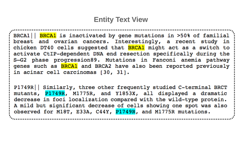
Figure 4: A toy example of constructing the entity text view. Original document view is the data provided by the Challenge. Entity text view is the extracted sentences from the overall documents globally that mentioned the specific gene or mutation. The entity texts for gene mutations are collected separately. The given example illustrates the view construction of a gene BRCA1 and its mutation P1749R. Then we can understand the knowledge not only from the document view but also from the entity text view.

3.2 Entity Text View

As we mentioned before, documents are too long and it would be helpful to analyze the view of texts containing individual genes or mutations. Correspondingly, we developed a two-step method including view construction and feature generation in the procedure of entity text view.

View Construction

Fig. 4 shows an illustrative example of entity text extraction. Basically, we firstly match strings with the names of gene or mutation in documents and then extract the sentences containing those strings. A trie tree-like fast string search algorithm named Aho-Corasick (AC) automaton AC is adopted. The complexity of the AC algorithm is linear $\mathcal{O}(n+m+z)$, where $n$, $m$ and $z$ are the length of the strings, the length of the texts, and the number of output matches, respectively. Without AC automaton, the time complexity of exact string matching is $\mathcal{O}(n+km)$ where $k$ is the number of patterns (genes or mutations in our scenario) that need to be found. Hence, it could take days to extract sentences with thousands of genes or mutations from original text to entity text, which is computationally prohibitive. As the computational complexity shown, AC automation is capable of solving the efficiency problem to a large extent.

Feature Generation

Once the sentences containing the names of gene or mutation are extracted, we collect all sentences mentioning a specific gene or a specific mutation as a separate entity text. Then the document feature engineering approaches introduced in the last subsection can be applied to these entity texts to generate feature vectors. Fortunately, both sentence-level features and word-level features show impressive performance on the top of entity texts. Note that the sentence-level TF-IDF is changed using the key sentences instead of context. Nevertheless, the document-level assumption of paragraph vector is not consistent with the entity view, since it lacks rationale to optimize the paragraph vector on the text without orderly sentences.

We concatenate the gene feature vector $\mathbf{x}^{ET}_{g}$ and mutation feature vector $\mathbf{x}^{ET}_{m}$ to get the combined feature vector $\mathbf{x}^{ET}=\mathbf{x}^{ET}_{g}||\mathbf{x}^{ET}_{m}$ for a specific gene mutation sample, as shown in Fig. 3. For instance, suppose a gene and a mutation are given, the n-gram feature for the given sample with a gene and a mutation is generated separately, on the basis of their corresponding extracted text. Then the concatenated n-gram vector can be used to represent the sample. The feature vector generated from entity text view is represented as $\mathbf{x}^{ET}$.

3.3 Entity Name View

Though most of the gene names and mutation names are short and only consist of few characters and numbers, the name itself contains useful information for classification. Two encoding approaches are designed to capture patterns from names, which are character-level n-gram and word embedding.

Character-Level Feature

Unlike word-level n-gram, we can set a large $n$ ($n=8$) as names are typically short strings. As a consequence, the feature dimension is extremely high. We adopt SVD to reduce the dimensionality to $20$. The other encoding approach uses label encoder to transform the letters and numbers in gene or mutation name into digital labels ($112$ unique labels in total) that can be used as feature directly.

Word Embedding Feature

Word embedding is a technique aiming at representing (embedding) words in a continuous vector space where semantically similar words are mapped to nearby points. Representative word embedding techniques include Word2Vec Word2Vec and GloVe GloVe . The trained word embedding models can offer us feature vector representations for each specific gene or mutation according to their names. In this task, we choose Word2Vec (Skip-Gram) skip-gram because both Word2Vec and GloVe achieve similar classification performance during the evaluation. The feature dimension of gene or mutation name vectors is set as $200$ according to cross-validation.

Similar to entity text view, the feature vector extracted from entity name view is concatenated by gene feature vector $\mathbf{x}^{EN}_{g}$ and mutation feature vector $\mathbf{x}^{EN}_{m}$, that is $\mathbf{x}^{EN}=\mathbf{x}^{EN}_{g}||\mathbf{x}^{EN}_{m}$. The feature vector generated from entity name view is represented as $\mathbf{x}^{EN}$.

3.4 Classifiers

Gradient Boosting Decision Tree (GBDT)  friedman2001greedy is a famous machine learning technique for regression and classification problems. Based on boosting, it aims to find an optimal model $f(\mathbf{x})$ that satisfies the following equation:

$$\hat{f}(\mathbf{x})=\arg\min_{f(\mathbf{x})}E[L(y,f(\mathbf{x}))|\mathbf{x}]$$ (2)

For a given dataset, $\mathbf{x}\in\mathbb{R}^{d}$ is an instance or a sample. Using an additive strategy similar to other ”boosting” paradigm, the functions $f(\mathbf{x})$ can be learned by the model:

$$\hat{f}(\mathbf{x})=\hat{f}_{K}(\mathbf{x})=\Sigma_{k=0}^{M}f_{k}(\mathbf{x})$$ (3)

where $f_{0}(\mathbf{x})$ is an initial guess and $\{f_{k}(\mathbf{x})\}_{1}^{K}$ are incremental functions. $\hat{f}(\mathbf{x})=\hat{f}_{K}(\mathbf{x}):\mathbb{R}^{d}\to\mathbb{R}$ is the objective function of the model. $K$ is the number of training iterations, which also equals to the number of boosted trees. Then the function $f_{k}(\mathbf{x})$ contains the structure of the tree and leaf scores, which is a weak classification model obtained at the $k$-th training iteration. In general, the tree boosting can be defined as the objective function $\mathcal{L}$ with a training loss term and regularization term:

$$\mathcal{L}=\Sigma_{i=1}^{N}l(y_{i},\Sigma_{k=0}^{M}f_{k}(\mathbf{x}_{i}))+\Sigma_{k=0}^{M}\Omega(f_{k})$$ (4)

where $N$ is the number of samples and $l$ is the logarithmic loss for multi-class classification in our scenario. To take advantages of feature vectors: $\mathbf{x}^{D}$, $\mathbf{x}^{ET}$, and $\mathbf{x}^{EN}$, we concatenate vectors from different views into a new vector $\mathbf{x}=\mathbf{x}^{D}\|\mathbf{x}^{ET}\|\mathbf{x}^{EN}$ Then the single-view classification models can be applied straightforwardly on the concatenated vector. The symbol $\|$ denotes concatenation operation on vectors from views.

In practice, we exploit two effective versions of gradient boosting algorithms: XGBoost and LightGBM. XGBoost has been proposed to use a second-order approximation by Taylor expansion of the loss function for the problem optimization chen2016xgboost . LightGBM can obtain a quite accurate estimation with smaller data size and fewer numbers of feature to speed up the conventional GBDT. Particularly, the specific gradient boosting algorithm in LightGBM we used is also GBDT. Through feature combinations across the given three views, multiple GBDT classifiers are trained independently.

Table 4: The details of feature combination for XGBoost models.

Model ID	Feature Combination
	Document View	Entity Text View	Entity Name View
GBDT_1	n/v/adj./adv. counts	n-gram+NMF	word embedding
	n/v/adj./adv. counts+NMF		character-level encoding
	n-gram+NMF
	bioentity counts
GBDT_2	paragraph vector	sentence-level TFIDF+SVD	word embedding
	sentence-level TFIDF+SVD		character-level encoding
	term frequency+LDA
	bioentity/keywords counts
GBDT_3	n/v/adj./adv. counts	sentence-level TFIDF+SVD	word embedding
	n/v/adj./adv.+NMF
	sentence-level TFIDF+SVD
	keywords counts
GBDT_4	n/v/adj./adv. TFIDF	n/v/adj./adv. TFIDF	word embedding
	sentence-level TFIDF+SVD		character-level encoding
	bioentity counts

Table 5: The details of feature combination for LightGBM models.

Model ID	Feature Combination
	Document View	Entity Text View	Entity Name View
GBDT_5	n/v/adj./adv. counts	n/v/adj./adv. TFIDF	word embedding
	n/v/adj./adv. counts+NMF
	n/v/adj./adv. TFIDF
GBDT_6	n-gram+NMF	n-gram+NMF	word embedding
	n/v/adj./adv. counts		character-level encoding
	n/v/adj./adv. counts+NMF
	bioentity counts
GBDT_7	n/v/adj./adv. TFIDF	n/v/adj./adv. TFIDF+SVD	word embedding
	n/v/adj./adv. counts+NMF
	sentence-level TFIDF+SVD
	n-gram+NMF
GBDT_8	sentence-level TFIDF+SVD	sentence-level TFIDF+SVD	word embedding
	n/v/adj./adv. counts		character-level encoding
	n/v/adj./adv. counts+NMF
	keywords counts
GBDT_9	n/v/adj./adv. TFIDF	n/v/adj./adv. TFIDF	word embedding
	sentence-level TFIDF+SVD		character-level encoding
	bioentity counts

4 Model Ensembles

Many existing successful machine learning stories on challenge solutions demonstrated that combining multiple models together can gain better performance than a single model NetflixChallenge ; Gesture . The rationale behind our framework is to combine features mined from original documents, entity texts, and entity names by different level features to form inputs of prediction models, and thus we can get numerous prediction results from these models (See Fig. 3). By setting a threshold to the logarithmic loss score ensemble , $9$ qualified models finally beat other models in the comparisons. Table 4 and 5 show the feature combinations used in training these models by XGBoost and LightGBM respectively. Based on the results of basic models, ensemble strategies of $2$ models, $3$ models, and $9$ models are applied. Through model ensemble, the system can eventually output a probability distribution over classes for each sample.

Formally, let $\hat{p}^{v}_{ij}$ be the final prediction result of validation data for sample $i$ of label $j$ and $\hat{p}^{s}_{ij}$ be the final prediction result of testing data for sample $i$ on label $j$. They are computed by the linear combination of results of single models as:

$$\hat{p}^{v}_{ij}=\Sigma_{c}\alpha_{c}\hat{p}^{v}_{ijc},\qquad\alpha_{c}>0$$ (5)

$$\hat{p}^{s}_{ij}=\Sigma_{c}\alpha_{c}\hat{p}^{s}_{ijc},\qquad\alpha_{c}>0$$

where $\hat{p}^{v}_{ijc}$ and $\hat{p}^{s}_{ijc}$ are the predicted probability of validation data and testing data by $c$-th single model. $i$ is the index of triplet $<g_{i},m_{i},d_{i}>$. $j$ is the index of class. $\alpha_{c}$ is the linear combination parameter for the $c$-th model, which is a positive weight.

Ensemble parameters $\alpha_{c}$ are computed by different manners: brute force grid searching and logarithmic loss minimization. The force grid searching quantizes the coefficient values in the interval $[0,1]$ at increments of $0.01$. It is an efficient way to find $\alpha$ when we need to ensemble $2$ or $3$ models. On the other hand, the logarithmic loss minimization problem on validation data can be mathematically defined as:

$$\alpha=\arg\min_{\alpha}\text{Logloss}(\Sigma_{c}\alpha_{c}\hat{p}^{v}_{c})$$ (6)

Followed the evaluation metric, the Logloss in our minimization problem is defined by:

$$\text{Logloss}=-\frac{1}{N}\Sigma_{i=1}^{N}\Sigma_{j=1}^{M}y_{ij}log(p_{ij})$$ (7)

where $N$ and $M$ are respectively the number of triplet $<g_{i},m_{i},d_{i}>$ observations and the number of class labels. As we can see, Eq. (7) is consistent with the evaluation metric in Eq. (1) provided by the Challenge. One limitation of the ensemble method is that it treats the classes with equal importance. However, after statistical analysis, we find that the $9$ classes are severely imbalanced. In order to overcome this limitation, we compute the loss on each class to optimize its own weight $\alpha_{cj}$. Based on the Eq. (6) and (7), the Logloss is updated by:

$$\text{Logloss}=-\Sigma_{j=1}^{M}\frac{1}{N_{j}}\Sigma_{i=1}^{N_{j}}y_{ij}log(p_{ij})$$ (8)

where $N_{j}$ is the number of triplet observations in the class $j$. The new Logloss can help us to learn weight $\alpha_{cj}$ for different classes and different models. Based on the improved ensemble method, we conduct a $9$ ensemble model.

5 Experimental Results

5.1 Experimental Settings

In the empirical study, we apply two offline test strategies. The first strategy is the stage-$1$ splitting which divides the entire samples into $3,321$ training samples and $368$ validation samples as shown in Table 2; the second strategy is $5$-fold cross validation on the overall $3,689$ samples. To verify the effectiveness, the evaluation metric logarithmic loss is used, which have been introduced in Section 2.

5.2 Effects of Multi-View Features

In our method, features mainly come from three different views. To test the effectiveness of single feature, XGBoost implementation is utilized. In Table 6, the features are fed into the $9$ basic gradient boosting models. Their dimensions and performance on $5$-fold cross-validation are shown. We test various bag-of-word and bag-of-n-gram features with or without dimension reduction methods, and there are $15$ winner features in total built on three views. In each view, the most effective single feature can be easily observed.

To compare two feature combinations of two views, we concatenate the features obtained by the same extraction methods, e.g., two feature vectors of term frequency+LDA are computed based on original documents and entity texts, respectively. Then we train GBDT models to test multi-view features by XGBoost implementation. Experimental results are presented in Table 7. Same feature derived from both document view and entity text view consistently outperforms the one only generated from a single view. The empirical study can demonstrate the effectiveness of using a complementary view.

Table 6: The dimensions and logarithmic loss scores obtained by the single feature in $3$ views on $5$-fold cross-validation (The classifier is implemented based on XGBoost).

Views	Feature	Dimension	5-fold cv
Document View	bioentity counts	10,022	0.9914
	keyword counts	3,379	0.9583
	Doc2Vec	400	1.0037
	sentence-level TFIDF+SVD	100	0.9939
	n/v/adj./adv. counts	9,868	1.0018
	n/v/adj./adv. TFIDF	9,868	0.9825
	n/v/adj./adv. counts+NMF	60	1.0417
	n-gram+NMF	60	1.0370
	term frequency+LDA	50	1.0348
Entity Text View	sentence-level TFIDF+SVD	200	0.9815
	n/v/adj./adv. TFIDF	9,868	0.9788
	n/v/adj./adv. TFIDF+SVD	200	1.0055
	n-gram+NMF	120	1.0029
Entity Name View	word embedding	200	0.9811
	character-level encoding	40	1.1031

Table 7: Result comparisons of feature generated from single view and double views on $5$-fold cross-validation. The double view contains document view and entity text view (The classifier is implemented based on XGBoost).

Feature	Single View	Double Views
n/v/adj./adv. TFIDF	0.9825	0.8558
sentence-level TFIDF+SVD	0.9939	0.8845
n/v/adj./adv. counts+NMF	1.0417	0.9029
n/v/adj./adv. TFIDF+SVD	1.0055∗	0.8775
term frequency+LDA	1.0348	0.9098

^∗ the score is based on feature in entity text view while others are computed in document view

5.3 Results of Basic Models

In the competition, $9$ different models are used in the model ensemble. Corresponding to the feature settings presented in Table 4 and 5, Table 8 and 9 show the results of basic gradient boosting models. For a fair comparison, all the models share the same setting of hyper-parameters. From the results, we can observe that GBDT models trained using XGBoost overall performs slightly better than those trained using LightGBM. Among the trained basic models using XGBoost, GBDT_3 has the best performance as a single model on $5$-fold cross-validation, while GBDT_2 has the best performance on stage-$1$ testing set. The situation for LightGBM is that GBDT_7 is superior to other models on $5$-fold cross-validation while GBDT_9 outperforms other models on stage-$1$ testing set.

.          Model Id          5-fold cv          Stage-1 test          GBDT_1          0.7068          0.5997          GBDT_2          0.6930          0.5638          GBDT_3          0.6870          0.5743          GBDT_4          0.6901          0.5657

Table 8: Results of GBDT model in terms of logarithmic loss on $5$-fold cross-validation and stage-$1$ testing set

Table 9: Results of GBM model in terms of logarithmic loss on $5$-fold cross-validation and stage-$1$ testing set.

Model Id	5-fold cv	Stage-1 test
GBDT_5	0.7005	0.6090
GBDT_6	0.7121	0.6152
GBDT_7	0.6967	0.6139
GBDT_8	0.7028	0.6178
GBDT_9	0.7001	0.6006

5.4 Results of Model Ensemble

Table 10: Results of 2 models ensemble by brute forcing grid search.

Model_1 Id	Model_2 Id	weight_1	weight_2	5-fold cv
GBDT_1	GBDT_4	0.4	0.6	0.6786
GBDT_6	GBDT_7	0.4	0.6	0.6846
GBDT_1	GBDT_7	0.4	0.6	0.6762

Table 11: Results of 3 models ensemble by brute forcing grid search.

Model_1 Id	Model_2 Id	Model_3 Id	weight_1	weight_2	weight_3	5-fold cv
GBDT_1	GBDT_2	GBDT_4	0.32	0.30	0.38	0.6738
GBDT_5	GBDT_6	GBDT_7	0.40	0.32	0.28	0.6818
GBDT_1	GBDT_4	GBDT_5	0.30	0.38	0.32	0.6695

Table 12: Results of 2 models ensemble by logarithmic loss minimization.

Model_1 Id	Model_2 Id	weight_1	weight_2	5-fold cv
GBDT_1	GBDT_4	0.49	0.51	0.6796
GBDT_6	GBDT_7	0.49	0.51	0.6860
GBDT_1	GBDT_7	0.49	0.51	0.6771

Table 13: Results of 3 models ensemble by logarithmic loss minimization.

Model_1 Id	Model_2 Id	Model_3 Id	weight_1	weight_2	weight_3	5-fold cv
GBDT_1	GBDT_3	GBDT_4	0.33	0.33	0.33	0.6745
GBDT_6	GBDT_8	GBDT_9	0.33	0.33	0.33	0.6832
GBDT_1	GBDT_4	GBDT_7	0.32	0.30	0.38	0.6718

Table 14: Results of the ensemble 9 models by logarithmic loss minimization.

Ensemble Method	stage-1 test	5-fold cv
LogLoss_Min	0.5547	0.6711
LogLoss_Min_cl	0.5506	0.6694

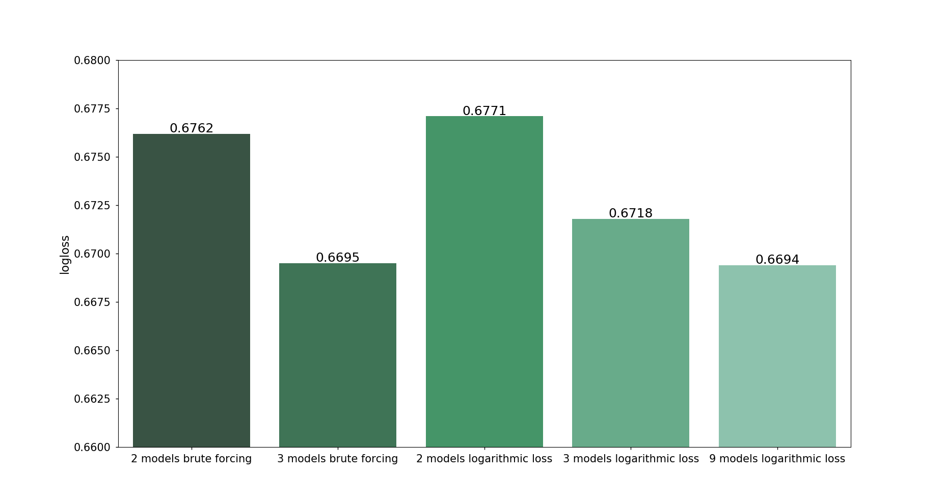
Figure 5: Experimental results of different model ensemble strategies on 5-fold cross validation.

Similarly, 5-fold cross-validation to the model ensemble is utilized here. In practice, brute force gird search strategy and logarithmic loss minimization strategy are used in the model ensemble. The combinations of basic models are shown in tables, if the evaluation of Logloss scores are less than a threshold. Table 10 and 11 respectively show ensemble results as well as weights by brute force grid search strategy to ensemble 2 models and 3 models.

Table 12 and 13 respectively show 2 and 3 ensemble results under the target of logarithmic loss minimization. The best model ensemble can be found in the results. The improved logarithmic loss minimization considering the imbalanced labels are also tested by $5$-fold cross-validation. The results in Table 14 show that the improved ensemble strategy can increase prediction accuracy on ensemble results of $9$ models. To compare the ensemble effects of $9$ models to $2$ models and $3$ models, the Fig. 5 plots the Logloss scores of main model ensemble methods concerned in this paper. Among different strategies, $9$ model ensemble is the final winner, which slightly outperforms the $3$ model ensemble based on brute forcing grid search.

6 Conclusion

The main contribution of our work is developing a comprehensive pipeline to perform gene mutation classification based on clinical articles. Our solution mines text features from three views including original document view, entity text view, and entity name view. Various machine learning algorithms are exploited to generate text features from perspectives of domain knowledge, document-level, sentence-level, and word-level. In addition, word embedding and character-level encoding based on entity names are adopted. Multiple GBDT classifiers with different feature combinations are utilized in ensemble learning to achieve a satisfying classification accuracy. The reported results demonstrate that our multi-view ensemble classification framework yields promising performances in this competition.

References

- [1] Alfred V Aho and Margaret J Corasick. Efficient string matching: an aid to bibliographic search. Communications of the ACM, 18(6):333–340, 1975.
- [2] Robert M. Bell and Yehuda Koren. Lessons from the netflix prize challenge. SIGKDD Explor. Newsl., 9(2):75–79, 2007.
- [3] David M Blei, Andrew Y Ng, and Michael I Jordan. Latent dirichlet allocation. Journal of machine Learning research, 3(Jan):993–1022, 2003.
- [4] Tianqi Chen and Carlos Guestrin. Xgboost: A scalable tree boosting system. In Proceedings of the 22nd acm sigkdd international conference on knowledge discovery and data mining, pages 785–794. ACM, 2016.
- [5] Christiane Fellbaum. WordNet. Wiley Online Library, 1998.
- [6] Jerome H Friedman. Greedy function approximation: a gradient boosting machine. Annals of statistics, pages 1189–1232, 2001.
- [7] Gene H Golub and Charles F Van Loan. Matrix computations, volume 3. JHU Press, 2012.
- [8] Zellig S Harris. Distributional structure. Word, 10(2-3):146–162, 1954.
- [9] Lin He, J Michael Thomson, Michael T Hemann, Eva Hernando-Monge, David Mu, Summer Goodson, Scott Powers, Carlos Cordon-Cardo, Scott W Lowe, Gregory J Hannon, et al. A microrna polycistron as a potential human oncogene. nature, 435(7043):828–833, 2005.
- [10] Minlie Huang, Jingchen Liu, and Xiaoyan Zhu. Genetukit: a software for document-level gene normalization. Bioinformatics, 27(7):1032–1033, 2011.
- [11] Dan Jurafsky and James H Martin. Speech and language processing, volume 3. Pearson London:, 2014.
- [12] Quoc Le and Tomas Mikolov. Distributed representations of sentences and documents. In Proceedings of the 31st International Conference on Machine Learning (ICML-14), pages 1188–1196, 2014.
- [13] Daniel D Lee and H Sebastian Seung. Learning the parts of objects by non-negative matrix factorization. Nature, 401(6755):788–791, 1999.
- [14] David AC Manning and JGM Decleer. Introduction to industrial minerals. 1995.
- [15] Grégoire Mesnil, Tomas Mikolov, Marc’Aurelio Ranzato, and Yoshua Bengio. Ensemble of generative and discriminative techniques for sentiment analysis of movie reviews. arXiv preprint arXiv:1412.5335, 2014.
- [16] Tomas Mikolov, Kai Chen, Greg Corrado, and Jeffrey Dean. Efficient estimation of word representations in vector space. arXiv preprint arXiv:1301.3781, 2013.
- [17] Tomas Mikolov, Ilya Sutskever, Kai Chen, Greg S Corrado, and Jeff Dean. Distributed representations of words and phrases and their compositionality. In Advances in neural information processing systems, pages 3111–3119, 2013.
- [18] Nanyun Peng, Hoifung Poon, Chris Quirk, Kristina Toutanova, and Wen-tau Yih. Cross-sentence n-ary relation extraction with graph lstms. arXiv preprint arXiv:1708.03743, 2017.
- [19] Jeffrey Pennington, Richard Socher, and Christopher Manning. Glove: Global vectors for word representation. In Proceedings of the 2014 conference on empirical methods in natural language processing (EMNLP), pages 1532–1543, 2014.
- [20] Sam T Roweis and Lawrence K Saul. Nonlinear dimensionality reduction by locally linear embedding. science, 290(5500):2323–2326, 2000.
- [21] Chih-Hsuan Wei, Bethany R Harris, Hung-Yu Kao, and Zhiyong Lu. tmvar: a text mining approach for extracting sequence variants in biomedical literature. Bioinformatics, 29(11):1433–1439, 2013.
- [22] Chih-Hsuan Wei and Hung-Yu Kao. Cross-species gene normalization by species inference. BMC bioinformatics, 12(8):S5, 2011.
- [23] Chih-Hsuan Wei, Hung-Yu Kao, and Zhiyong Lu. Pubtator: a web-based text mining tool for assisting biocuration. Nucleic acids research, 41(W1):W518–W522, 2013.
- [24] Jiaxiang Wu, Jian Cheng, Chaoyang Zhao, and Hanqing Lu. Fusing multi-modal features for gesture recognition. In Proceedings of the 15th ACM on International Conference on Multimodal Interaction, pages 453–460, 2013.
- [25] Xiang Zhang, Junbo Zhao, and Yann LeCun. Character-level convolutional networks for text classification. In Advances in neural information processing systems, pages 649–657, 2015.