Analysis of Invariance and Robustness via Invertibility of ReLU-Networks

Abstract

Studying the invertibility of deep neural networks (DNNs) provides a principled approach to better understand the behavior of these powerful models. Despite being a promising diagnostic tool, a consistent theory on their invertibility is still lacking. We derive a theoretically motivated approach to explore the preimages of $\operatorname{ReLU}$-layers and mechanisms affecting the stability of the inverse. Using the developed theory, we numerically show how this approach uncovers characteristic properties of the network.

1 Introduction

While there has been a growing effort to rigorously study the mathematics behind deep neural networks (DNNs), see (Vidal et al., 2017) for an overview, their inner workings are only sparsely understood so far. Although many open questions have been tackled – like the expressive power of neural networks (Raghu et al., 2017), the matter of generalization (Zhang et al., 2017) and the difficulties of optimizing a non-convex loss landscape (Choromanska et al., 2015) – the inner workings of a particular network is often at best partially understood. Besides a given model’s performance on the test set the interpretation of its decisions (Montavon et al., 2018) and the analysis of its sensitivity to adversarial perturbations (Szegedy et al., 2014) are key steps to assess the nature of its behavor.
Despite of, or maybe due to, the relevancy of adversarial examples, it is of similar importance to better our understanding of the opposite effect: Which perturbations $\Delta x$ do not (or only little) affect the outcome of the network $F$? This question can be addressed for a given input datapoint $x$ via searching for all $\Delta x$, such that

$$F(x)=F(x+\Delta x)\quad\text{(invariant) or}\quad\|F(x)-F(x+\Delta x)\|\leq\varepsilon\quad\text{(robust)},$$

where a small $\varepsilon>0$ is given. These properties can be crucial for many discriminative tasks in order to contract the space along uninformative directions (Mallat, 2016). However, a model would be flawed if perturbations that alter the semantics only have a minor impact on the features of the network. In Figure 1 such examples are shown, where perturbations entirely change its semantics while all the network’s features – even the first layer’s – are exactly the same for the original and perturbed image.
A natural way to address these properties is by studying the invertibility: If $F$ is invariant to perturbations $\Delta x$, then $x$ and $\Delta x$ lie in the preimage of the output $z=F(x)$ i.e. $F$ is not uniquely invertible. Robustness towards large perturbations induces an instable inverse mapping as small changes in the output can be due to large changes in the input. Most notably, this analysis is dual to adversarial examples (Szegedy et al., 2014) where small perturbations induce large changes in the outcome, which shows instabilities in the forward mapping.
In this work we address the issue of invariance via analyzing preimages and studying the stability of the inverse mapping. Besides the importance of understanding the behavior of a model, further applications of studying the inverse include: input reconstruction (Mahendran and Vedaldi, 2015) (Mahendran and Vedaldi, 2016) to backtrack properties from feature space to input space or inverse problems with learned forward models (Jensen et al., 1999) (Lu et al., 1999). As the approximation capabilities of neural networks were recently even used to learn solutions of partial differential equations (Sirignano and Spiliopoulos, 2017), parameter estimation problems often formulated as inverse problems would require the inversion of networks.

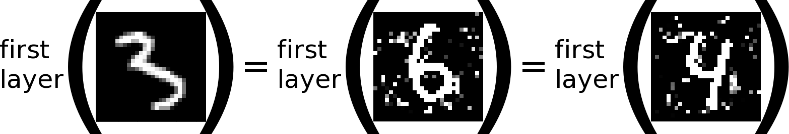
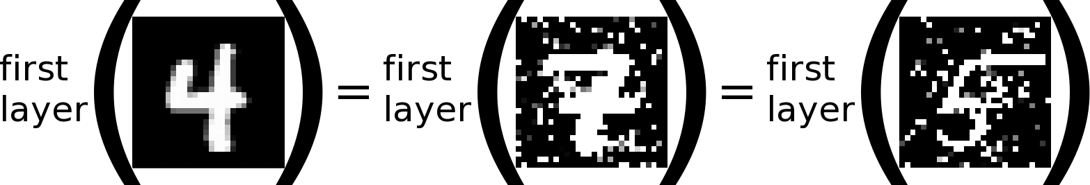
Figure 1: Invariances of the first layer (100 $\operatorname{ReLU}$ neurons) of a vanilla multilayer perceptron (MLP). Despite the semantically very different examples, the features are identical as the original image "3" and the two perturbed variants "6" and "4" are in the same preimage. Further details in Appendix A7.

1.1 Related Work and Contributions

While analyzing invariance and robustness properties is a major topic in theoretical treatments of deep networks (Mallat, 2016), studying it via the inverse is less common. Several works like (Mahendran and Vedaldi, 2015) or (Dosovitskiy and Brox, 2016) focus on reconstructing inputs from features of convolutional neural networks (CNNs) to visualize the information content of features. Instead, we investigate potential mechanisms affecting the invertibility. (Carlsson et al., 2017) gives a first geometrical view on the shape of preimages of outputs from $\operatorname{ReLU}$ layers, which is directly related to the question of injectivity of the mapping under $\operatorname{ReLU}$. (Shang et al., 2016) analyzes the reconstruction property of cReLU (concatenated $\operatorname{ReLU}$); however, the more general situation of using the standard rectifier is not studied. A notable other line of work assumes random weights in order to derive guarantees for invertibility, see (Gilbert et al., 2017) or (Arora et al., 2015), whereas we aim to theoretically derive means to uncover mechanisms of rectifier networks without assumptions on the weights.
Moreover, several reversible network structures were recently proposed (Gomez et al., 2017) (Chang et al., 2018) (Jacobsen et al., 2018). Most notably, in (Jacobsen et al., 2018) a bijective network, up to its last layer, was trained successfully on ImageNet which does not exhibit any invariance. However, the network is very robust towards many directions in the input which is reflected in a strongly instable inverse. Hence, even carefully designed network show at least one of the two effects (invariance and robustness) studied in this work. Especially stability has seen growing interest due to adversarial examples (Szegedy et al., 2014), yet stability is mostly studied with respect to the forward mapping, see e.g. (Cisse et al., 2017).
Two main resources for our view of rectifier networks as piecewise linear models are (Montufar et al., 2014) and (Raghu et al., 2017). Closest to our approach is the work of (Bruna et al., 2014) on global statements of injectivity and stability of a single layer including $\operatorname{ReLU}$ and pooling. The authors focus on global injectivity and stability bounds via combinatorial statements over all configurations attainable by $\operatorname{ReLU}$ and pooling. These conditions are valid on the entire input space, while the restriction to parts of the input space may be far from these worst-case conditions.
Our contributions are as follows:

• We provide computable conditions when the preimage of an output point for one $\operatorname{ReLU}$-layer is finite, infinite or a single point (injective). In contrast to (Bruna et al., 2014), where conditions are given for all input points, we refine this locally for a single point. Afterwards we numerically investigate the properties of preimages for a trained network. (See Section 2.)

• We study the stability of the inverse via analyzing the linearization at a point in input space, which is accurate within a polytope. We provide upper bounds on the smallest singular value and prove how the removal of uncorrelated features could effect the stability of the inverse mapping. Furthermore, we provide numerical results showing the (in-)stability of the inverse of rectifier networks. (See Section 3.)

1.2 Notation

Input: $x=x^{0}\in\mathbb{R}^{d_{0}}$, sometimes shortened to $d:=d_{0}$. • Pre-activations: $z^{l}=A^{l}x^{l-1}+b^{l}\in\mathbb{R}^{d_{l}},$ with weight matrix $A^{l}\in\mathbb{R}^{d_{l}\times d_{l-1}}$ and bias $b^{l}\in\mathbb{R}^{d_{l}}$.

Activation: $x^{l}=\phi(z^{l})\in\mathbb{R}^{d_{l}},$ where $\phi:\mathbb{R}\to\mathbb{R}$ the pointwise applied activation function, if not specified differently $g:=\operatorname{ReLU}$. • Number of layers: $L\in\mathbb{N}$

• Entire network: $F:\mathbb{R}^{d}\ni x\mapsto F(x):=z:=z^{L}\in\mathbb{R}^{d_{L}}$, sometimes short $D:=d_{L}$.

For matrices $A\in\mathbb{R}^{m\times n}$ and $I\subset[m]:=\{1,\dots,m\}$, $A|_{I}$ denotes the matrix consisting of the rows of $A$ whose index is in set $I$ – analogously for vectors. Also $A|_{y>0}$ describes the restriction to the index set $\{i:y_{i}>0\}$ for $y\in\mathbb{R}^{m}$, analogously for $<,=,\leq,\geq$. For vectors $y\in\mathbb{R}^{m}$, $y>0$ is the elementwise relation, analogously for $<,=,\leq,\geq$. Furthermore, we define $\mathcal{N}(A)$ as the null space of the matrix $A.$
For every matrix $A\in\mathbb{R}^{m\times n}$ with the rows $a_{i}$, $i\in[m]$, we associate the set $A=\{a_{i}\}_{i=1}^{m}$. Vice versa, we associate every finite set in $\mathbb{R}^{n}$ with a matrix (only possible up to permutation of the indices).

2 Preimages of ReLU Layer

2.1 Theoretical Analysis

In this section, we analyze different kinds of preimages of a $\operatorname{ReLU}$-layer and investigate under which conditions the inverse image of a given point is a singleton (a set containing exactly one element) or has finite/infinite volume. These conditions will yield a simple algorithm able to distinguish between these different preimages, which is applied in Section 2.2.
For the analysis of pre-images of a given output one can study single layers separately or multiple layers at once. However, since the concatenation of two injective functions is again injective while a non-injective function followed by an injective function is non-injective, studying single layers is crucial. We therefore develop a theory for the case of single layers in this section. Notice that in case of multiple layers one is also required to investigate the image space of the previous layer.
We will focus our study on the most common activation function, $\operatorname{ReLU}$. One of its key features is the non-injectivity, caused by the constant mapping on the negative half space. It provides neural networks with an efficient way to deploy invariances. Basically all other common activation functions are injective, which would lead to a straightforward analysis of the preimages. However, injective activations like ELU Clevert et al. (2016) and Leaky ReLU Maas et al. (2013) only swap the invariance for robustness, which in turn leads to the problem of having instable inverses. This question of stability will be analyzed in more detail in Section 3.
We start by introducing one of our main tools – namely the omnidirectionality.

Definition 1 (Omnidirectionality)

1. $A\in\mathbb{R}^{m\times n}$ is called omnidirectional if there exists a unique $x\in\mathbb{R}^{n},$ such that $Ax\leq 0$ (component-wise).

2. $A\in\mathbb{R}^{m\times n}$ and $b\in\mathbb{R}^{m}$ are called omnidirectional for the point $p\in\mathbb{R}^{n}$ if $A$ is omnidirectional and $b=-Ap.$

Corollary 2

The following statements are equivalent:

1. $A\in\mathbb{R}^{m\times n}$ is omnidirectional.

2. Every linear open halfspace in $\mathbb{R}^{n}$ contains a row of $A$.

3. $Ax\leq 0$ implies $x=0$, where $x\in\mathbb{R}^{n}$.

Figure 2: Gray lines are hyperplanes with normal vectors (arrows) from the rows of $A$ and translation $b$. Left: Omnidirectional tuple $(A,b)$ for $p\in\mathbb{R}^{2}$, as hyperplanes intersect in $p$ and normal vectors are omnidirectional. Two in the middle: Intersection in $p$, but vector-free halfspaces (hence, not omnidirectional). Right: hyperplanes do not intersect in a point, but normal vectors are omnidirectional.

Thus, for every direction of a hyperplane through the origin forming two halfspaces, there is a vector from the rows of $A$ inside each open halfspace, hence the term omnidirectional (see Figure 2 for an illustration). Note that the hyperplanes are due to $\operatorname{ReLU}$ as it maps the open halfspace to positive values and the closed halfspace to zero. A straightforward way to construct an omnidirectional matrix is by taking a matrix whose rows form a spanning set $\mathcal{F}$ and use the vertical concatenation of $\mathcal{F}$ and $-\mathcal{F}$. This idea is realated to cReLU Shang et al. (2016).
More importantly, omnidirectionality is directly related to the $\operatorname{ReLU}$-layer preimages and will provide us with a computable method to characterize their volume (see Theorem 4). To analyze such inverse images, we consider

$$y=\operatorname{ReLU}(Ax+b)$$ (1)

for a given output $y\in\mathbb{R}^{m}$ with $A\in\mathbb{R}^{m\times n}$, $b\in\mathbb{R}^{m}$ and $x\in\mathbb{R}^{n}.$ If we know $A,b$ and $y$, we can write (1) as the following mixed linear system:

$$A|_{y>0}x+b|_{y>0} =y|_{y>0}$$ (2)

$$A|_{y=0}x+b|_{y=0} \leq 0.$$ (3)

Remark 3

It is possible to enrich the mixed system to include conditions/priors on $x$ (e.g. $x\in\mathbb{R}^{n}_{\geq 0}$).

The inequality system in (3) links its set of solutions and therefore the volume of the preimages of the $\operatorname{ReLU}$-layer with the omnidirectionality of $A$ and $b.$ Defining $\overline{A}\coloneqq AO^{T},$ where $O\in\mathbb{R}^{k\times n}$ denotes an orthonormal basis of $\operatorname{\mathcal{N}}(A|_{y>0})$ with $k:=\dim\operatorname{\mathcal{N}}(A|_{y>0})$ and $\overline{b}:=b|_{y\leq 0}+A|_{y\leq 0}(P_{\operatorname{\mathcal{N}}(A|_{y>0})^{\perp}}x)$ leads to the following main theorem of this section, which is proven in Appendix A1.

Theorem 4 (Preimages of $\operatorname{ReLU}$- layer)

The preimage of a point under a $\operatorname{ReLU}$-layer is a

1. singleton, if and only if there exists an index set $I$ for the rows of $\overline{A}$ and $\overline{b},$ such that $(\overline{A}|_{I},\overline{b}|_{I})$ is omnidirectional for some point $p\in\mathbb{R}^{n}.$

2. compact polytope with finite volume, if and only if $\overline{A}$ is omnidirectional.

Thus, omnidirectionality allows in theory to distinguish whether the inverse image of a $\operatorname{ReLU}$-layer is a singleton, a compact polytope or has infinite volume. However, obtaining a computable method to decide whether a given matrix is omnidirectional is crucial for later numerical investigations. For this reason, we will go back to the geometrical perspective of omnidirectionality (see Figure 2). This will also help us to get a better intuition on the frequency of occurence of the different preimages. The following Theorem 5 gives another geometrical interpretation of omnidirectionality besides Corollary 2ii, whose short proof is given in Appendix A1.

Theorem 5 (Convex hull)

A matrix $A\in\mathbb{R}^{m\times n}$ is omnidirectional if and only if $0\in{\kern 0.0pt\operatorname{Conv}(A)}^{\mathrm{o}},$ where ${\kern 0.0pt\operatorname{Conv}(A)}^{\mathrm{o}}$ is the interior of the convex hull spanned by the rows of $A$ (see Definition 11 in Appendix A1).

Therefore, the matrix must contain a simplex in order to be omnidirectional, as the convex hull of the matrix $A\in\mathbb{R}^{m\times n}$ has to have an interior. Hence, we have the following:

Corollary 6

If $A\in\mathbb{R}^{m\times n}$ is omnidirectional, then $m>n.$

Considering the geometric perspective that the tuple $(A\in\mathbb{R}^{m\times n},b\in\mathbb{R}^{m})$ is omnidirectional for a point $p\in\mathbb{R}^{n},$ if and only if the $m$ hyperplanes generated by the rows of $A$ with bias $b$ intersect at $p$ and their normal vectors (rows of $A$) form an omnidirectional set. We can use Corollary 6 to conclude that singleton preimages of $\operatorname{ReLU}$-layers are very unlikely to happen in practice (if we do not design for it), since a necessary condition is that $n+1$ hyperplanes have to intersect in one point in $\mathbb{R}^{n}.$ Therefore we conclude, that singleton preimages of $\operatorname{ReLU}$ layers in practice only and exclusively occurs, if the mixed linear system already has sufficient linear equalities.
Furthermore, the above results can be used to derive an algorithm to check whether a preimage of a given output is finite, infinite or just a singleton. A singleton inverse image is obtained as long as $\operatorname{rank}(A|_{y>0})=n$ holds true, which can be easily computed. To distinguish preimages with finite and infinite volumes, it is enough to check if $\overline{A}$ is omnidirectional (see Theorem 4ii), which can be done numerically by using the definition of the convex hull, Theorem 5 and Corollary 6. This leads to a linear programming problem, which is presented in Appendix A3.

2.2 Numerical Analysis

In this subsection we demonstrate for a simple model that the preimage of a layer can be a singleton, infinite or finite depending on the given point. For this purpose, we trained a MLP with two hidden $\operatorname{ReLU}$ layers of size $3500$ and $784$ and a 10 neuron softmax output layer on MNIST LeCun and Cortes (2010). We chose the layer size of $3500$, because the likelihood of having roughly $784$ (input dimension of MNIST) positive outputs was high for this setting. In Figure 4, we plotted how many samples of the test set have infinite (red curve) or finite (blue curve) preimages over the number of positive outputs. It can be assumed that all samples which have more or equal to 784 (the input dimension) positive outputs have a singleton preimage and are therefore finite. In the dark gray region between $723$ and $784$, both effects occurred, which can be seen by the overlap of the red and blue curve.
To determine whether a preimage for less than 784 positive outputs was compact we used Theorem 4ii and the algorithm described in Appendix A3.
We also conducted first experiments whether the compactness of the pre-image has an influence on the range of manipulations à la Figure 1. However, compact pre-images only occurred in cases where the number of positive outputs resulted in a linear system which already determined the image up to a level where manipulations were imperceptible. A thorough study is left for future work.

Figure 3: Removal of vectors due to $\operatorname{ReLU}$ (red crosses) for the marked points $x$ (left:unbiased setting, right: biased setting). The remaining vectors are only weakly correlated to the removed one, thus yielding an unstable inverse.

Figure 4: The number of (in-)finite volumed preimages of a $\operatorname{ReLU}$ layer over the test set of MNIST. Only within the gray strip we see finite and infinite volumed preimages.

3 Stability

3.1 Theoretical Analysis

In this section we analyze the robustness of rectifier MLPs against large perturbations via studying the stability of the inverse mapping. Concretely, we study the effect of $\operatorname{ReLU}$ on the singular values of the linearization of network $F$. While the linearization of a network $F$ at some point $x$ only provides a first impression on its global stability properties, the linearization of $\operatorname{ReLU}$ networks is exact in some neighborhood due to its piecewise-linear nature (Raghu et al., 2017). In particular, the input space $\mathbb{R}^{d}$ of a rectifier network $F$ is partitioned into convex polytopes $P_{F}$, corresponding to a different linear function on each region. Hence, for each polytope $P$ in the set of all input polytopes $P_{F}$, the network $F$ can be simplified as $F(x)=A_{P}x+b_{P}$ for all $x\in P$.
Additionally, each of these matrices $A_{P}$ can be written via a chain of weight matrix multiplications incorporating the effect of $\operatorname{ReLU}$, see (Wang et al., 2016). In particular let $D_{I}$ denote a diagonal matrix with $D_{ii}=1$ for $i\not\in I$ and $D_{ii}=0$ for $i\in I$. Then $A_{P}$ of a network with $L$ layers can be written as

$$A_{P}=A^{L}D_{I^{L-1}}A^{L-1}\cdots D_{I^{1}}A^{1},$$

where $A^{l}$ are the weight matrices of layer $l$ and $I^{l}:=\{i\in[d_{l}]:(A^{l}x^{l-1}+b^{l})_{i}\leq 0\}$. Thus, the effect of $\operatorname{ReLU}$ is incorporated in the diagonal matrices $D_{I^{l}}$ which set the rows of $A^{l}$ with indices from $I^{l}$ to zero. For the purpose of studying all possible local behaviors, we define admissible index sets $I^{l}$ following, with slight modifications, (Bruna et al., 2014):

Definition 7

(Admissible index sets)
An index set $I^{l}$ for a layer $l$ is admissible if

$$\bigcap_{i\not\in I^{l}}\{x^{l}:\langle x^{l},a^{l}_{i}\rangle>-b_{i}\}\cap\bigcap_{i\in I^{l}}\{x^{l}:\langle x^{l},a^{l}_{i}\rangle\leq-b_{i}\}\neq\emptyset.$$

Of special interest for such an analysis is the range of possible effects by the application of the rectifier. Since the effect by $\operatorname{ReLU}$ corresponds to the application of $D_{I}$ for admissible $I$, we now turn to studying the changes of the singular values due to $D_{I}$. By considering the matrix $A$, e.g. representing the chain of matrix products up to layer $l$, the effect of $\operatorname{ReLU}$ can be globally upper bounded:

Lemma 8

(Global upper bound for largest and smallest singular value)
Let $\sigma_{l}$ be the singular values of $D_{I}A$. Then for all admissible index sets $I$, the smallest non-zero singular value is upper bounded by

$$\min\{\sigma_{l}:\sigma_{l}>0\}\leq\tilde{\sigma}_{k},$$

where $k=N-|I|$ and $\tilde{\sigma}_{1}\geq...\geq\tilde{\sigma}_{N}>0$ are the non-zero singular values of $A$.
Furthermore, the largest singular value is upper bounded by

$$\max\{\sigma_{l}:\sigma_{l}>0\}\leq\tilde{\sigma}_{1}.$$

Lemma 8 analyzes the best case scenario with respect to the highest value of the smallest singular value. While this would yield a more stable inverse mapping, one needs to keep in mind that the nullspace $\operatorname{\mathcal{N}}(A_{P})$ grows by the corresponding elimination of rows via $D_{I}$. Moreover, reaching this bound is very unlikely as it requires the singular vectors to perfectly align with the directions that collapse due to $D_{i}$. Thus, we now turn to study effects which could happen locally for some input polytopes $P$.
An example of a drastic effect through the application of $\operatorname{ReLU}$ is depicted in Figure 4. Since one vector is only weakly correlated to the removed vector and the situation is overdetermined, removing this feature for some inputs $x$ in the blue area leaves over the strongly correlated features. While the two singular values of the 3-vectors-system were close to one, the singular vectors after the removal by $\operatorname{ReLU}$ are badly ill-conditioned. As many modern deep networks increase the dimension in the first layers, redundant situations as in Figure 4 are common, which are inherently vulnerable to such phenomena. For example, (Rodríguez et al., 2017) proposes a regularizer to avoid such strongly correlated features. The following lemma formalizes the situation exemplified before:

Lemma 9

(Removal of weakly correlated rows)
Let $A\in\mathbb{R}^{m\times n}$ with rows $a_{j}$ and $I\subseteq[m]$. For a fixed $k\in I$ let $a_{k}\in\operatorname{\mathcal{N}}(D_{I}A)^{\bot}$. Moreover, let

$$\forall j\not\in I:|\langle a_{j},a_{k}\rangle|\leq c\frac{\|a_{k}\|_{2}}{\sqrt{M}},$$ (4)

with $M=m-|I|$ and constant $c>0$. Then for the singular values $\sigma_{l}\neq 0$ of $D_{I}A$ it holds

$$0<\sigma_{K}=\min\{\sigma_{l}:\sigma_{l}\neq 0\}\leq c.$$

(Note that $I$ has to be admissible when considering the effect of $\operatorname{ReLU}$.)

Lemma 9 provides an upper bound on the smallest singular value, given a condition on the correlation of all $a_{j}$ and $a_{k}$. However, the condition (4) depends on the number $N$ of remaining rows $a_{j}$. Hence, in a highly redundant setting even after removal by $\operatorname{ReLU}$ (large $N$), $c$ needs to be large such that the correlation fulfills the condition. Yet, in this case the upper bound on the smallest singular value, given by $c$, is high. We discuss this effect further in the Appendix A5.
We now turn our attention to the effect of multiple layers and ask whether the use of multiple layers results in a different situation than a 1-hidden layer MLP. In particular: Can the application of another layer have a pre-conditioning effect yielding a stable inverse? What happens when we only compose orthogonal matrices which have stable inverses? Note that a way to enforce an approximate orthogonality constraint was proposed for CNNs in (Cisse et al., 2017), however only for the filters of the convolution.
For both situations the answer is similar: the nonlinear nature of $\operatorname{ReLU}$ induces locally different effects. Loosely speaking, we apply the layer $A^{l}$ to different linearizations depending on the input region $P$. Thus, if we choose a pre-conditioner $A^{l}$ for a specific matrix $A^{l-1}_{P}$, it might not stabilize the matrix product for matrices $A^{l-1}_{P^{*}}$ corresponding to different input polytopes $P^{*}$. For the case of composing only orthogonal matrices, consider a network up to layer $l-1$ where the linearization $A^{l-1}_{P}$ has orthogonal columns (assume the network gets larger, thus $A^{l-1}_{P}$ has more rows than columns). Then, the application of $\operatorname{ReLU}$ in form of

$$A^{l}D_{I^{l}}A^{l-1}_{P}$$ (5)

removes the orthogonality property of the rows of $A^{l-1}_{P}$, if setting entries in the rows from $I^{l}$ to zero results in non-orthogonal columns. This effect is likely, especially when considering dense matrices, hence $D_{I^{l}}A^{l-1}_{P}$ is for some $I^{l}$ not orthogonal. Thus, the matrix product 5 is not orthogonal, resulting in decaying singular values.
This is why, even when especially designing the network by e.g. orthogonal matrices, stability issues with respect to the inverse arise. To conclude this section, we remark that the presented results are rather of a qualitative nature showcasing effects of $\operatorname{ReLU}$ on the singular values. Yet, the analysis does not require any assumptions and is thus valid for any MLP (including CNNs without pooling). To give an idea of quantitative effects we study numerical examples in the subsequent subsection.

3.2 Numerical Analysis

In this section we conduct simple experiments on CIFAR10 Krizhevsky and Hinton (2009) to numerically study the stability of CNNs. We simplify the CNNs by using only strides instead of pooling, and furthermore use no residual connections and batch-normalization layers. Thus, the architectures fit to the theoretical study as the strided discrete convolution can be written as a matrix-vector multiplication. Details on the used CNNs and training setup are in Appendix A4. Furthermore, we remark that the linearization of a network $F$ for an input point $x^{0}$ can be computed via backpropagation.
Using the linearization obtained by backpropagation, we proceed by computing the SVD. In particular, we are interested in the entire distribution of singular values. Computing all singular values is numerically expensive and scales with the input and output size of the linearized network. Especially, early CNN-layers have high dimensional outputs which may cause memory issues when computing the entire SVD. We thus choose a small CNN trained on CIFAR10 as these inputs are only of size $32\times 32\times 3$. In order to scale this analysis up to e.g. ImageNet with VGG-networks, a restriction to a window of the input image is necessary in order to compute the full SVD of early layers. See (Jacobsen et al., 2018), where the singular values restricted to input windows were used to estimate the stability of the entire i-RevNet trained on ImageNet.

Effect of $\operatorname{ReLU}$: We start the evaluation by looking into the effect of $\operatorname{ReLU}$ on the singular values of a layer. In the theoretical section, Lemma 9 considered the case of removal of weakly correlated rows. In these situations, $\operatorname{ReLU}$ could remove rows of the weight matrices resulting in drastically smaller singular values after $\operatorname{ReLU}$. However, as Figure 6 shows for the layers 2 and 5 of WideCIFAR, this effect is not present in this example. In this figure, the decay of the median singular values is shown using 50 samples from the CIFAR10 test set propagated until layer 2 and 5. The blue and red lines correspond to the linearization without $\operatorname{ReLU}$-activation, while the green and turquoise lines are singular values after $\operatorname{ReLU}$. While $\operatorname{ReLU}$ results in smaller singular values, as discussed in the upper bounds in Lemma 8, they are only slightly smaller. To better understand this effect, we numerically compute the conditions from Lemma 9 and discuss the implications in Appendix A5. In summary from the results in the appendix, the above example is too redundant to exhibit strong effects due to removal of rows.

Effect of multiple layers: We now move to the development of the singular values over several layers. Figure 6 shows the decay in convolutional layers (layers 1-6, after application of $\operatorname{ReLU}$). While the shape of the curve is similar for layer 1-5, it can be seen that the largest singular value grows, while the small singular values decrease significantly. Note that this growth of the largest singular values is in line with observations for adversarial examples, see (Szegedy et al., 2014). While many defense strategies like (Cisse et al., 2017) or (Jia, 2017) focus on the largest singular value, the behavior of the smaller singular values are of special interest for the stability of the inverse. Another effect to note, is the cut-off curve for layer 6 in yellow. Here there are way fewer singular values than in previous layers. This is caused by the downsampling in this layer by strided convolution and the row removal by $\operatorname{ReLU}$.
The same experiments were conducted for ThinCIFAR and for the MLP from Section 2.2, see Appendix A6.

Trade-off between stability and invariance: In the example above, it could be seen that the inverse for layer 6 would be more stable, while there are many invariance directions (zero singular value). To further investigate this trade-off, Figure 7 compares the output size, the condition number and the number of non-zero singular values vs. the layers for WideCIFAR and ThinCIFAR. In combination with lower output dimension, $\operatorname{ReLU}$ has a different effect for ThinCIFAR. The number of singular values decreases in layer 5, which cuts off the smallest singular values, resulting in a lower condition number. On the other hand, there are more directions where the network is invariant within the corresponding linear region.
In conclusion, these experiments showed how $\operatorname{ReLU}$ affects the singular value decay and exposed a trade-off between stability and information loss. This study investigated only small networks on MNIST and CIFAR10, in order to reduce computational costs. However, a study on larger networks and datasets would be of great interest and is left for future work.

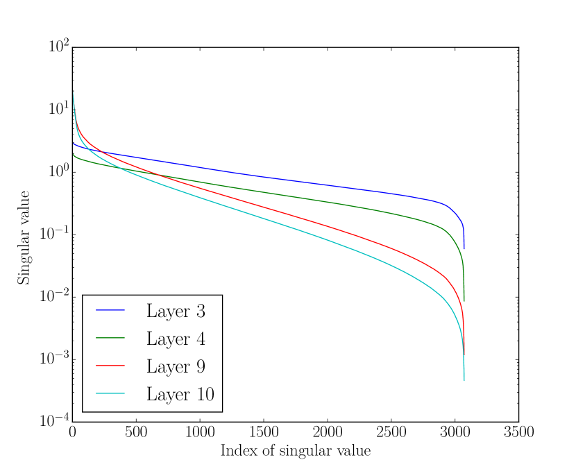
Figure 5: Effect of $\operatorname{ReLU}$ on the singular values for WideCifar. The curves show the effect in layer 2 (layer 3 and 4 in the legend, because $\operatorname{ReLU}$ is counted as an extra activation layer) and layer 5 (layer 9 and 10), where each curve is the median over 50 samples.

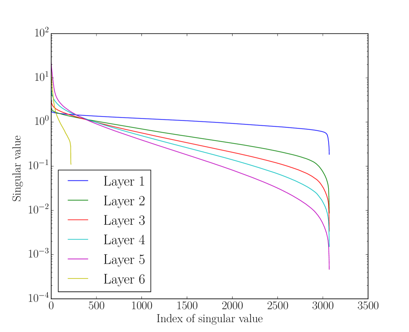
Figure 6: Decay of singular values over the layers of the network. Here, each layer includes the convolution and $\operatorname{ReLU}$-activation. Reported number are taken from median over 50 samples.

Figure 7: In blue are the results from WideCIFAR and in red ThinCIFAR. Top: number of output units per layer, Middle: number of singular values, Bottom: Behavior of condition number, each curve over the layers. Here, layers are split into conv-layer and $\operatorname{ReLU}$-activation layer. Singular values and condition number are the median over 50 samples from the CIFAR10 test set.

4 Conclusion and Outlook

We presented a approach to better understand the invariance and robustness properties of $\operatorname{ReLU}$ networks via studying its inverse. Our analysis yielded computable conditions under which the preimage of a $\operatorname{ReLU}$ layer is a point, finite or infinite. We showed how to analyze the inverse stability using the singular values of the linearization. This view provided insights into mechanisms that effect stability and allowed simple experiments to study properties of the inverse of CNNs.
Most noticeable, our analysis lays a well founded starting point for further studies on robustness and invariance properties. In future work we plan to further investigate methods to construct examples from the preimage of features deeper in the network (invariance) or finding large perturbations which do little effect (robustness). Furthermore, a more accurate analysis of the inverse stability should incorporate nonlinear effects like moving between linear regions of rectifier networks. In addition, our study considered general weight matrices, whereas a restriction to CNNs might enable a tighter theoretical analysis. Finally, studying the invertibility could be of major interest in the context of inverse problems with forward models learned by neural networks.

5 Acknowledgments

We thank Emily King and Christian Etmann for helpful discussions and feedback on the draft and Dmitry Feichtner-Kozlov for pointing out Stiemke’s theorem. Furthermore, we gratefully acknowledge the financial support from the German Science Foundation for RTG 2224 "$\pi^{3}$: Parameter Identification - Analysis, Algorithms, Applications".

A1 Appendix for Section 2

Corollary 10

For $A\in\mathbb{R}^{m\times n}$ the following statements are equivalent.

1. $A$ is omnidirectional.

2. $\nexists x\neq 0:Ax\leq 0$

3. $\nexists x\gneq 0:Ax\leq 0$

4. Every linear open halfspace contains a row of $A$.

5. $Ax\leq 0$ implies $x=0$.

Here $z\lneq 0$ means $z\in\mathbb{R}^{n}_{\leq 0}$ and $z\neq 0$.

Definition 11

(Convex hull)
For $A\in\mathbb{R}^{m\times n},$ the convex hull is defined as

$$\operatorname{Conv}(A)=\left\{\sum_{i=1}^{m}\alpha_{i}a_{i}:\forall i\ \alpha_{i}\in\mathbb{R}_{\geq 0}\land\sum_{i}\alpha_{i}=1\right\},$$

where $a_{i}\in\mathbb{R}^{n}$ are the rows of $A$.

Theorem 12

(Stiemke’s theorem e.g. Dantzig [1963])
Let $A\in\mathbb{R}^{m\times n}$ be a matrix, then the following two expressions are equivalent.

• $\nexists y:Ay\lneq 0$

• $\exists x>0:A^{T}x=0$

Here $z\lneq 0$ means that $0\neq z\leq 0$ .

Theorem 13

(Singleton solutions of inequality systems)
Let $A\in\mathbb{R}^{m\times n}$, $b\in\mathbb{R}^{m}$ and $x\in\mathbb{R}^{n}$. Furthermore, let the inequality system

$$Ax+b\leq 0,$$

written as $(A,b)$, have a solution $x_{0}$.
Then this solution is unique if and only if there exists an index set, $I$, for the rows s.t. $(A|_{I},b|_{I})$ is omnidirectional for $x_{0}$.

Proof  (Theorem 13, Singleton solutions of inequality systems)
“$\Leftarrow$”
Let $(A|_{I},b|_{I})$ be omnirectional for $x_{0}.$ Then it holds that $A|_{I}x+b|_{I}=A|_{I}(x-x_{0})\leq 0.$ Due to the omnidirectionality of $A|_{I},$ $x_{0}$ is the unique solution of the inequality system $A|_{I}x+b|_{I}\leq 0.$ The existence of a solution for the whole system $Ax+b\leq 0$ is guaranteed by assumption and therefore $x_{0}$ is the unique solution of $Ax+b\leq 0.$
“$\Rightarrow$”
Here we will proove

$$\text{``}\nexists I:(A|_{I},b|_{I})\text{ omnidirectional for some $p$ }\Rightarrow\text{ solution non-unique}\text{''}.$$

We will start by doing the following logical transformations:

$$\phantom{\Leftrightarrow\ \ }\nexists I:(A|_{I},b|_{I})\text{ omnidirectional for some $p$ }$$

$$\Leftrightarrow\nexists(I,p):(A|_{I}\text{ omnidirectional}\land b|_{I}=-A|_{I}p)$$

$$\Leftrightarrow\forall(I,p):\lnot(A|_{I}\text{ omnidirectional}\land b|_{I}=-A|_{I}p)$$

$$\Leftrightarrow\forall(I,p):(A|_{I}\text{ not omnidirectional}\lor b|_{I}\neq-A|_{I}p).$$

Now we define the vector $c_{0}:=Ax_{0}+b\leq 0$ and the set $I$ as the index set given via $c_{0}=0$.

This means that $A|_{I}$ is not omnidirectional, because otherwise $A|_{I}x_{0}+b|_{I}=0$ due to the definition of $I,$ which would lead to the contradiction that $(A|_{I},b|_{I})$ is omnidirectional for $x_{0}.$ But this means $\exists x^{\prime}\neq 0:A|_{I}x^{\prime}\leq 0$ as a result of Corollary 10. Since $A|_{I^{c}}x_{0}+b|_{I^{c}}<0,$ we also have $\forall x\ \ \exists\epsilon>0:A|_{I^{c}}(x_{0}+\epsilon x)+b|_{I^{c}}<0.$ This holds in particular for $x^{\prime},$ so we define accordingly $x^{*}:=\varepsilon x^{\prime}\neq 0.$ Therefore, we have $A|_{I^{c}}(x_{0}+x^{*})+b|_{I^{c}}<0$ as well as

$$A|_{I}(x_{0}+x^{*})+b_{I}=\underbrace{A|_{I}x_{0}+b_{I}}_{=c_{0}=0}+\underbrace{\varepsilon A|_{I}x^{\prime}}_{\leq 0}\leq 0.$$

Altogether it holds that $A(x_{0}+x^{*})+b\leq 0$ with $x^{*}\neq 0,$ which means that $x_{0}$ is a non-unique solution for the inequality system $Ax+b\leq 0.$   $\square$

Proof (Theorem 4, Preimages of $\operatorname{ReLU}$-layers)
We consider the $\operatorname{ReLU}$-layer

$$y=\operatorname{ReLU}(Ax+b),$$

given its output $y\in\mathbb{R}^{m}$ with $A\in\mathbb{R}^{m\times n}$, $b\in\mathbb{R}^{m}$ and $x\in\mathbb{R}^{n}.$ Clearly, this equation can also be written as the mixed linear system

$$A|_{y>0}x+b|_{y>0} =y|_{y>0},$$

$$A|_{y=0}x+b|_{y=0} \leq 0.$$

This allows us to consider the two cases

$$\operatorname{\mathcal{N}}(A|_{y>0})=\{0\}\text{ and }\operatorname{\mathcal{N}}(A|_{y>0})\neq\{0\}.$$

In the first case, we have a linear system which allows us to calculate $x$ uniquely, i.e. we can do retrieval. This leads us to the second case, the interesting one. In this case we can only recover $x$ uniquely if and only if the system of inequalities “pins down” $P_{\operatorname{\mathcal{N}}(A|_{y>0})}x$, where $P_{V}$ is the orthogonal projection into the closed space $V$. Formally this requires

$$A|_{y\leq 0}(P_{\operatorname{\mathcal{N}}(A|_{y>0})^{\perp}}x+P_{\operatorname{\mathcal{N}}(A|_{y>0})}x)+b|_{y\leq 0}\leq 0$$

to have a unique solution for $x\in\mathbb{R}^{n}$ and $P_{\operatorname{\mathcal{N}}(A|_{y>0})^{\perp}}x$ fixed (given via the equality system). By defining $\overline{b}:=b|_{y\leq 0}+A|_{y\leq 0}(P_{\operatorname{\mathcal{N}}(A|_{y>0})^{\perp}}x)$ we have

$$A|_{y\leq 0}(P_{\operatorname{\mathcal{N}}(A|_{y>0})}x)+\overline{b}\leq 0.$$

If $O\in\mathbb{R}^{k\times n}$ now denotes an orthonormal basis of $\operatorname{\mathcal{N}}(A|_{y>0})$, where $k:=\dim\operatorname{\mathcal{N}}(A|_{y>0})$, we can write

$$\overline{A}\overline{x}+\overline{b}\leq 0,$$

where $\overline{A}:=AO^{T}$ and $\overline{x}:=Ox$ is a general element in $\mathbb{R}^{k}$. It now follows from Theorem13 that the inequality system $(\overline{A},\overline{b})$ has a unique solution if and only if $(\overline{A},\overline{b})$ has a subset of rows that are omnidirectional for some point $p$.   $\square$

Proof  (Theorem 5, Convex hull theorem)
Since $\operatorname{\mathcal{N}}(A)=\{0\}$ follows from both sides of the equivalence, the following sequence of equivalencies holds. $0\in{\kern 0.0pt\operatorname{Conv}(A)}^{\mathrm{o}}$ $\Leftrightarrow$ $\exists x>0:A^{T}x=0$ $\xLeftrightarrow{\text{Theorem \ref{thm_stiemke}}}$ $\nexists y:Ay\lneq 0$ $\xLeftrightarrow{\text{Corollary~{}\ref{corollary_omnidirectional} and $\operatorname{\mathcal{N}}(A)=\{0\}$}}$ $\nexists y\neq 0:Ay\leq 0$   $\square$

A2 Proofs for section 3

Proof (Proof of Lemma 8, Global upper bound for largest/smallest singular value)
The upper bound on the largest singular value is trivial, as $\operatorname{ReLU}$ is contractive or in other terms $\|D_{I}Ax\|_{2}\leq\|Ax\|_{2}$ for all $I$ and $x\in\mathbb{R}^{n}$.
To prove the upper bound for the smallest singular value, we assume

$$\sigma_{M}:=\min\{\sigma_{l}:\sigma_{l}>0\}>\tilde{\sigma}_{k}$$ (6)

and aim to produce a contradiction. Consider all singular vectors $\tilde{v}_{k^{*}}$ with $k^{*}\geq k$ from matrix $A$. It holds for all $\tilde{v}_{k^{*}}$

$$\tilde{\sigma}_{k}\geq\tilde{\sigma}_{k^{*}}=\|A\tilde{v}_{k^{*}}\|_{2}\geq\|D_{I}A\tilde{v}_{k^{*}}\|_{2},$$ (7)

as $D_{I}$ is a projection matrix and thus only contracting. As

$$\sigma_{M}=\min_{\begin{subarray}{c}\|x\|_{2}=1\\ x\in\mathcal{N}(D_{I}A)^{\bot}\end{subarray}}\|D_{I}Ax\|_{2},$$

all $\tilde{v}_{k^{*}}\not\in\mathcal{N}(D_{I}A)^{\bot}$. Otherwise, a $\tilde{v}_{k^{*}}$ would be a minimizer by estimation (7), which would violate the assumption (6).

Due to $\mathcal{N}(D_{I}A)^{\bot}\oplus\mathcal{N}(D_{I}A)=\mathbb{R}^{n}$, it holds $\tilde{v}_{k^{*}}\in\mathcal{N}(D_{I}A)$. As $\tilde{v}_{k^{*}}$ are orthogonal, $\text{dim}(span(v_{k^{*}}))=|I|+1$ (note: $k^{*}=k,...,N$ and $k=N-|I|$, thus there are $|I|+1$ singular vectors $v_{k^{*}}$ in total). Furthermore, $\tilde{v}_{k^{*}}$ were not in $\mathcal{N}(A)$ by definition (corresponding singular values were strictly positive).
Hence, the nullspace of $D_{I}$ must have $\text{dim}(\mathcal{N}(D_{I}))\geq|I|+1$. But $D_{I}$ is the identity matrix except $|I|$ zeros on the diagonal, thus $\text{dim}(\mathcal{N}(D_{I}))=|I|$, which yields a contradiction.   $\square$

Proof (Proof of Lemma 9, Weakly correlated rows)
Consider $v=\frac{a_{k}}{\|a_{k}\|_{2}}$. Then,

$$(D_{I}Av)_{k}=0,$$

since $k\in I$ ($k$-th row of $D_{I}$ is zero). Furthermore, for all $j\neq k$ it holds by condition (4)

$$(D_{I}Av)_{j}=\frac{\langle a_{k},a_{j}\rangle}{\|a_{k}\|_{2}}\leq\frac{|\langle a_{k},a_{j}\rangle|}{\|a_{k}\|_{2}}\leq\frac{c}{\sqrt{M}}.$$

Hence,

$$\|D_{I}Av\|_{2}=\sqrt{\sum_{j\not\in I}\left(\frac{\langle a_{k},a_{j}\rangle}{\|a_{k}\|_{2}}\right)^{2}}\leq\sqrt{M\left(\frac{c}{\sqrt{M}}\right)^{2}}=c.$$

As $a_{k}\in\mathcal{N}(D_{I}A)^{\bot}$, $v\in\mathcal{N}(D_{I}A)^{\bot}$ as well. Thus,

$$\sigma_{K}=\min_{\begin{subarray}{c}\|x\|_{2}\\ x\in\mathcal{N}(D_{I}A)^{\bot}\end{subarray}}\|D_{I}A\|_{2}\leq\|D_{I}Av\|_{2}\leq c.$$

$\square$

A3 Appendix for Section 2.2

In this section, we formulate the algorithm to determine whether the preimage of $y$ given by

$$y=\operatorname{ReLU}(Ax+b)$$

is finite.
This requires to check whether $\overline{A}$ (see Theorem 4) is omnidirectional, which is equivalent to

$$0\in{\kern 0.0pt\operatorname{Conv}(\overline{A})}^{\mathrm{o}},$$

see Theorem 5. Since it is reasonable to assume that $0$ will not lie on the boundary of the convex hull, we can formulate this as a linear programming problem. The side-conditions incorporate the definition of convex hulls (Definition 11, Appendix A1). The objective function is chosen arbitrary, as we are only interested in a solution.

Algorithm 1 Finite preimage

  Input: $A\in\mathbb{R}^{m\times n}$, $b\in\mathbb{R}^{m}$, $y\in\mathbb{R}^{m}$

  if $\operatorname{rank}(A|_{y>0})=n$ then

     return True {Preimage is a singleton}

  end if

  $O\leftarrow$ orthonormal basis of $\operatorname{\mathcal{N}}(A|_{y>0})$, ($\in\mathbb{R}^{k\times n}$)

  $\overline{A}\leftarrow A|_{y=0}O^{T}$, ($\in\mathbb{R}^{\tilde{k}\times k}$)

  if $\tilde{k}\leq k$ then

     return False {see Corollary 6}

  end if

  $c\leftarrow(1;\dots;1)$ {arbitrary objective}

  return Does a solution for the linear program $\begin{cases}\mbox{max}\ c^{T}x\\ \text{subject to}\\ \hskip 28.45274pt\overline{A}^{T}x=0\\ \hskip 28.45274pt(1;\dots;1)^{T}x=1\\ \hskip 28.45274ptx\in[0,1]^{\tilde{k}}\end{cases}$ exists?

A4 Architectures for Numerical Studies

Training details for MLP on MNIST:

• Training using Adam optimizer [Kingma and Ba, 2015]

• Epochs: 25

• Batch size: 1000

Training details for WideCIFAR and ThinCIFAR:

• Training setup from Keras [Chollet et al., 2015] examples: cifar10_cnn

• No data augmentation

• RMSprop optimizer

• Epochs: 100

• Batch size: 32

Table 1: Architecture of MLP trained on MNIST

Index	Type	kernel size	stride	# feature maps	# output units
0	Input layer	-	-	3
1	Dense layer	-	-	-	100
2	Dense layer	-	-	-	100
3	Dense layer	-	-	-	100
4	Dense layer	-	-	-	100
5	Dense layer	-	-	-	100
6	Dense layer	-	-	-	100
7	Dense layer	-	-	-	100
8	Dense layer	-	-	-	100
9	Dense layer	-	-	-	100
10	Dense layer	-	-	-	100
11	Dense layer (softmax)	-	-	-	10

Table 2: Architecture of MLP trained on MNIST

Index	Type	kernel size	stride	# feature maps	# output units
0	Input layer	-	-	3
1	Dense layer	-	-	-	3500
2	Dense layer	-	-	-	784
3	Dense layer (softmax)	-	-	-	10

Table 3: Architecture of WideCIFAR

Index	Type	kernel size	stride	# feature maps	# output units
0	Input layer	-	-	3
1	Convolutional layer	(3,3)	(1,1)	32	-
2	Convolutional layer	(3,3)	(2,2)	64	-
3	Convolutional layer	(3,3)	(1,1)	64	-
4	Convolutional layer	(3,3)	(1,1)	32	-
5	Convolutional layer	(3,3)	(1,1)	32	-
6	Convolutional layer	(3,3)	(2,2)	64	-
7	Dense layer	-	-	-	512
8	Dense layer (softmax)	-	-	-	10

Table 4: Architecture of ThinCIFAR

Index	Type	kernel size	stride	# feature maps	# output units
0	Input layer	-	-	3
1	Convolutional layer	(3,3)	(1,1)	32	-
2	Convolutional layer	(3,3)	(2,2)	32	-
3	Convolutional layer	(3,3)	(1,1)	16	-
4	Convolutional layer	(3,3)	(1,1)	16	-
5	Convolutional layer	(3,3)	(1,1)	16	-
6	Convolutional layer	(3,3)	(2,2)	32	-
7	Dense layer	-	-	-	512
8	Dense layer (softmax)	-	-	-	10

A5 Numerical Analysis of Lemma 9

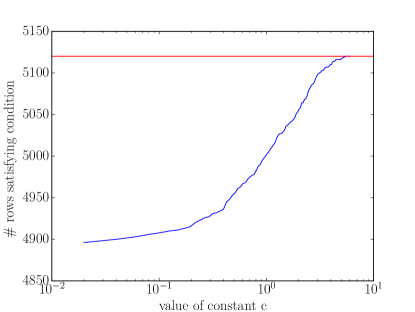
Figure 8: Curve showing how many rows $a_{i}$ satisfy condition (4) from Lemma 9 depending on values of constant $c$. The red line shows the total number of remaining rows after removal by $\operatorname{ReLU}$, $M=5120$. Even for small constants $c$ most $a_{i}$ fulfill condition (4), yet not all, which is required by the lemma to give an upper bound on the smallest singular value. The example is from layer 4 of WideCIFAR, for only one sample from the test set.

In order to better understand the bound on the smallest singular value after $\operatorname{ReLU}$, given by Lemma 9, we numerically proceed as follows:

1. We choose $c\in[a,b]$, where $a,b$ are suitable interval endpoints.

2. Given $c$, we compute for every $a_{k}$ with $k\in I$ the value of $c\frac{\|a_{k}\|_{2}}{\sqrt{M}}$ ($M$ is the number of remaining rows, in the example $M=5120$).

3. For every $a_{k}$ we count the number of $a_{i}$ satisfying

   $$|\langle a_{i},a_{k}\rangle|\leq c\frac{\|a_{k}\|_{2}}{\sqrt{M}}.$$

4. We take the $a_{k}$ with the maximal number of $a_{i}$ satisfying the condition. (Note, that this ignores the requirement $a_{k}\in\operatorname{\mathcal{N}}(D_{I}A)^{\bot}$.)

5. If we have an $a_{k}$, where all $a_{i}$ satisfy the condition, the corresponding constant $c$ gives the upper bound on the smallest singular value after $\operatorname{ReLU}$.

Figure 8 shows the number of $a_{i}$ satisfying the correlation condition given different choices of $c$. The red line is reached for $c\approx 6$. However, even the largest singular value after $\operatorname{ReLU}$ is smaller than 2.5 (shown in Figure 6). Thus, the bound given by Lemma 9 is far off. This can be explained by the fact, that this situation is quite redundant ($M=5120$) and there are rows $a_{i}$ still correlated to the removed rows $a_{k}$.
However, in the further Experiments on ThinCIFAR, we observe (see Figure 10) a stronger effect of $\operatorname{ReLU}$ in layer 2, which can be explained by having a less redundant scenario with fewer remaining rows.

A6 Further Experiments

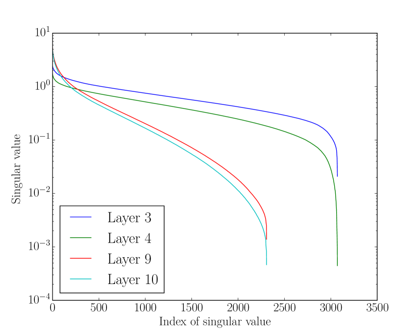
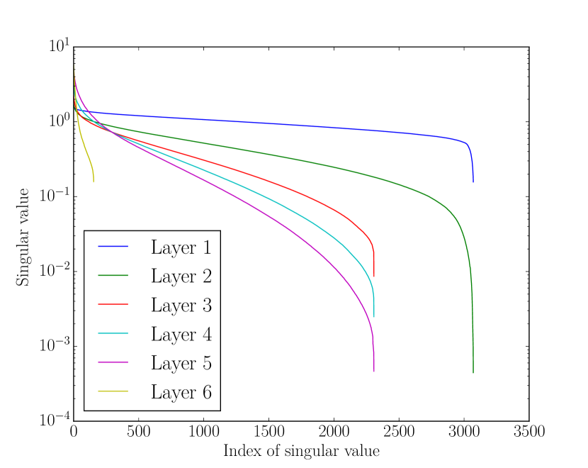
Figure 9: Left: Effect of $\operatorname{ReLU}$ on the singular values for ThinCifar. The curves show the effect in layer 2 (layer 3 and 4 in legend, because $\operatorname{ReLU}$ is counted as an extra activation layer) and layer 5 (layer 9 and 10). Right: Decay of singular values over the layers ThinCifar. Here, each layer includes the convolution and $\operatorname{ReLU}$-activation. Reported number are taken from median over 50 samples. Best viewed in color.

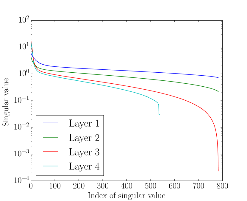
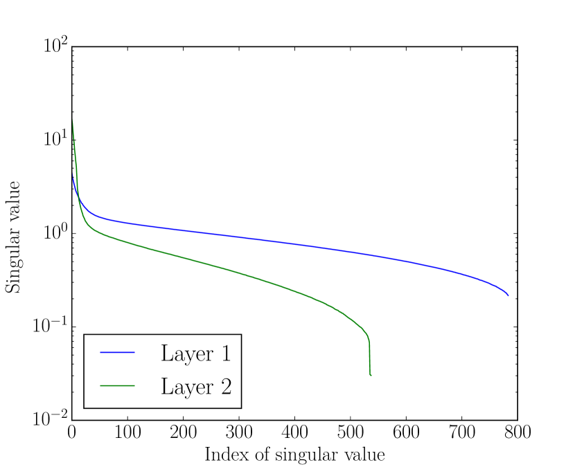
Figure 10: Left: Effect of $\operatorname{ReLU}$ on the singular values for the MLP on MNIST. The curves show the effect in layer 1(layer 1 and 2 in legend, because $\operatorname{ReLU}$ is counted as an extra activation layer) and layer 2 (layer 3 and 4). Right: Decay of singular values over the layers of MLP on MNIST. Here, each layer includes the fully-connected layer and $\operatorname{ReLU}$-activation. Reported number are taken from median over 50 samples.

A7 Invariance Experiment using an MLP on MNIST

This section briefly describes how the results in Figure 1 from the introduction were obtained (copied in Figure 11 for readability). After training the network from 1 (in Appendix A4), we searched the MNIST test set for input images with yielded the fewest positive activations in the first layer, in the figure the digits "3" and "4". After selecting the example input $x^{*}$, we selected another input $c$ belonging to a different class (e.g. a "6" and "4" in the first example).
Afterwards, we solved following linear programming problem to find a perturbed $x$:

$$\begin{cases}\mbox{max}\ \langle c,x\rangle\\ \text{subject to}\\ \hskip 28.45274ptA|_{y^{*}>0}x+b|_{y^{*}>0}=y^{*}|_{y^{*}>0}\\ \hskip 28.45274ptA|_{y^{*}<0}x+b|_{y^{*}<0}\leq 0\\ \hskip 28.45274ptx\in[0,1]^{\tilde{k}}\end{cases},$$

where the features of the first layer are computed via

$$y^{*}=\operatorname{ReLU}(Ax^{*}+b).$$

Hence, we searched within the preimage of the features $y^{*}$ of the first layer for examples $x$ which resemble images $c$ from another class. By doing this we observe, that the preimages of the MLP may have large volume. In these cases, the network is invariant to some semantics changes which shows how the study of preimages can reveal previously unknown properties.

Figure 11: Invariances of the first layer (100 $\operatorname{ReLU}$ neurons) of a vanilla MLP. (Exact architecture in Appendix A4 Table 1.)

References

- Arora et al. (2015) S. Arora, Y. Liang, and T. Ma. Why are deep nets reversible: a simple theory, with implications for training. arXiv preprint, arXiv:1511.05653, 2015.
- Bruna et al. (2014) J. Bruna, A. Szlam, and Y. LeCun. Signal recovery from pooling representations. In Proceedings of the 31st International Conference on Machine Learning, 2014.
- Carlsson et al. (2017) S. Carlsson, H. Azizpour, A. Razavian, J. Sullivan, and K. Smith. The preimage of rectifier activities. In International Conference on Learning Representations (workshop), 2017.
- Chang et al. (2018) B. Chang, L. Meng, E. Haber, L. Ruthotto, D. Begert, and E. Holtham. Reversible architectures for arbitrarily deep residual neural networks. The Thirty-Second AAAI Conference on Artificial Intelligence, 2018.
- Chollet et al. (2015) F. Chollet et al. Keras. https://github.com/keras-team/keras, 2015.
- Choromanska et al. (2015) A. Choromanska, M. Henaff, M. Mathieu, G. Ben Arous, and Y. LeCun. The loss surfaces of multilayer networks. In Proceedings of the Eighteenth International Conference on Artificial Intelligence and Statistics, volume 38, 2015.
- Cisse et al. (2017) M. Cisse, P. Bojanowski, E. Grave, Y. Dauphin, and N. Usunier. Parseval networks: improving robustness to adversarial examples. In Proceedings of the 34 International Conference on Machine Learning, 2017.
- Clevert et al. (2016) D.-A. Clevert, T. Unterthiner, and S. Hochreiter. Fast and accurate deep network learning by exponential linear units (elus). International Conference on Learning Representations, 2016.
- Dantzig (1963) G. Dantzig. Linear programming and extensions. Princeton University Press, 1963.
- Dosovitskiy and Brox (2016) A. Dosovitskiy and T. Brox. Inverting convolutional networks with convolutional networks. In Proceedings of IEEE Conference on Computer Vision and Pattern Recognition, 2016.
- Gilbert et al. (2017) A. Gilbert, Y. Zhang, K. Lee, Y. Zhang, and H. Lee. Towards understanding the invertibility of convolutional neural networks. In 26th International Joint Conference on Artificial Intelligence, 2017.
- Gomez et al. (2017) A. N. Gomez, M. Ren, R. Urtasun, and R. B. Grosse. The reversible residual network: backpropagation without storing activations. In Advances in Neural Information Processing Systems 30, 2017.
- Jacobsen et al. (2018) J.-H. Jacobsen, A. W. Smeulders, and E. Oyallon. i-revnet: deep invertible networks. In International Conference on Learning Representations, 2018.
- Jensen et al. (1999) C. A. Jensen, R. D. Reed, R. J. Marks, M. A. El-Sharkawi, J.-B. Jung, R. T. Miyamoto, G. M. Anderson, and C. J. Eggen. Inversion of feedforward neural networks: algorithms and applications. In Proceedings of the IEEE, volume 87(9), pages 1536–1549, 1999.
- Jia (2017) K. Jia. Improving training of deep neural networks via singular value bounding. IEEE Conference on Computer Vision and Pattern Recognition, 2017.
- Kingma and Ba (2015) D. P. Kingma and J. Ba. Adam: a method for stochastic optimization. Proceedings of the 32nd International Conference on International Conference on Machine Learning, 2015.
- Krizhevsky and Hinton (2009) A. Krizhevsky and G. Hinton. Learning multiple layers of features from tiny images, 2009.
- LeCun and Cortes (2010) Y. LeCun and C. Cortes. MNIST handwritten digit database, 2010. URL http://yann.lecun.com/exdb/mnist/.
- Lu et al. (1999) B.-L. Lu, H. Kita, and Y. Nishikawa. Inverting feedforward neural networks using linear and nonlinear programming. IEEE Transactions on Neural Networks, 10(6):1271–1290, 1999.
- Maas et al. (2013) A. L. Maas, A. Y. Hannun, and A. Y. Ng. Rectifier nonlinearities improve neural network acoustic models. In Proceedings of the 30th International Conference on Machine Learning, 2013.
- Mahendran and Vedaldi (2015) A. Mahendran and A. Vedaldi. Understanding deep image representations by inverting them. In In Proceedings of IEEE Conference on Computer Vision and Pattern Recognition, 2015.
- Mahendran and Vedaldi (2016) A. Mahendran and A. Vedaldi. Visualizing deep convolutional neural networks using natural pre-images. International Journal of Computer Vision, 120(3):233–255, 2016.
- Mallat (2016) S. Mallat. Understanding deep convolutional networks. Philosophical Transactions of the Royal Society of London A: Mathematical, Physical and Engineering Sciences, 374(2065), 2016. ISSN 1364-503X. doi: 10.1098/rsta.2015.0203. URL http://rsta.royalsocietypublishing.org/content/374/2065/20150203.
- Montavon et al. (2018) G. Montavon, W. Samek, and K.-R. Müller. Methods for interpreting and understanding deep neural networks. Digital Signal Processing, 73, 2018.
- Montufar et al. (2014) G. F. Montufar, R. Pascanu, K. Cho, and Y. Bengio. On the number of linear regions of deep neural networks. In Advances in Neural Information Processing Systems 27, 2014.
- Raghu et al. (2017) M. Raghu, B. Poole, J. Kleinberg, S. Ganguli, and J. Sohl-Dickstein. On the expressive power of deep neural networks. In Proceedings of the 34th International Conference on Machine Learning, 2017.
- Rodríguez et al. (2017) P. Rodríguez, J. Gonzàlez, G. Cucurull, J. M. Gonfaus, and F. X. Roca. Regularizing cnns with locally constrained decorrelations. In International Conference on Learning Representations, 2017.
- Shang et al. (2016) W. Shang, K. Sohn, D. Almeida, and H. Lee. Understanding and improving convolutional neural networks via concatenated rectified linear units. In Proceedings of the 33rd International Conference on Machine Learning, 2016.
- Sirignano and Spiliopoulos (2017) J. Sirignano and K. Spiliopoulos. Dgm: a deep learning algorithm for solving partial differential equations. arXiv preprint, arXiv:1708.07469, 2017.
- Szegedy et al. (2014) C. Szegedy, W. Zaremba, I. Sutskever, J. Bruna, D. Erhan, I. J. Goodfellow, and R. Fergus. Intriguing properties of neural networks. International Conference on Learning Representations, 2014.
- Vidal et al. (2017) R. Vidal, J. Bruna, R. Giryes, and S. Soatto. Mathematics of deep learning. arXiv preprint, arXiv:1712.04741, 2017.
- Wang et al. (2016) S. Wang, A. rahman Mohamed, R. Caruana, J. Bilmes, M. Plilipose, M. Richardson, K. Geras, G. Urban, and O. Aslan. Analysis of deep neural networks with extended data jacobian matrix. In Proceedings of the 33rd International Conference on Machine Learning, 2016.
- Zhang et al. (2017) C. Zhang, S. Bengio, M. Hardt, B. Recht, and O. Vinyals. Understanding deep learning requires rethinking generalization. International Conference on Learning Representations, 2017.