On the Cosmological Implications of the String Swampland

Abstract

We study constraints imposed by two proposed string Swampland criteria on cosmology. These criteria involve an upper bound on the range traversed by scalar fields as well as a lower bound on $|\nabla_{\phi}V|/V$ when $V>0$. We find that inflationary models are generically in tension with these two criteria. Applying these same criteria to dark energy in the present epoch, we find that specific quintessence models can satisfy these bounds and, at the same time, satisfy current observational constraints. Assuming the two Swampland criteria are valid, we argue that the universe will undergo a phase transition within a few Hubble times. These criteria sharpen the motivation for future measurements of the tensor-to-scalar ratio $r$ and the dark energy equation of state $w$, and for tests of the equivalence principle for dark matter.

1 Introduction

The landscape of string theory gives a vast range of choices for how our universe may fit in a consistent quantum theory of gravity. However, it is believed that this is surrounded by an even bigger Swampland, i.e., a set of consistent looking effective quantum field theories coupled to gravity, which are inconsistent with a quantum theory of gravity [1]. For a recent review of the subject and references see [2]. The aim of this paper is to investigate the cosmological implications of two of the proposed Swampland criteria.

The two Swampland criteria whose consequences we will study are:

Criterion 1: The range traversed by scalar fields in field space is bounded by $\Delta\sim{\cal{O}}(1)$ in reduced Planck units [3]. More precisely, consider a theory of quantum gravity coupled to a number of scalars $\phi^{i}$ in which the effective Lagrangian, valid up to a cutoff scale $\Lambda$, takes the form

$$\mathcal{L} =\sqrt{|g|}\left[\frac{1}{2}R-\frac{1}{2}g^{\mu\nu}\partial_{\mu}\phi^{i}\partial_{\nu}\phi^{j}G_{ij}(\phi)\right.$$

$$\qquad\qquad\qquad\qquad\qquad\qquad\left.-V(\phi)+\ldots\frac{}{}\right],$$ (1)

where we use reduced Planck units throughout. Note in particular that we go to the Einstein frame and use $G_{ij}(\phi)$ in this frame to define a metric which we use to measure distances in the field space $\phi^{i}$. Then it is believed that there is a finite radius in field space where the effective Lagrangian above is valid. In particular if we go a large distance $D$ in field space, a tower of light modes appear with mass scale

$$m\sim M_{pl}\exp(-\alpha D)$$ (2)

which invalidates the above effective Lagrangian. Here $\alpha\sim{\cal O}(1)$. This means that any effective Lagrangian has a proper field range for $|\Delta\phi|<\Delta$, where the expectation is that $\Delta\sim{\cal O}(1)$. There is by now a lot of evidence for this conjecture. See in particular [4, 5, 6] for a recent discussion and extensions of this conjecture.

Criterion 2: There is a lower bound $|\nabla_{\phi}V|/V>c\sim{\cal O}(1)$ in reduced Planck units in any consistent theory of gravity when $V>0$. The second Swampland criterion, which was recently conjectured in [7], is motivated by the observation that it appears to be difficult to construct any reliable dS vacua and by experience with string constructions of scalar potentials.

We will be applying these two criteria to periods of possible cosmic acceleration. In particular we revisit early universe inflationary models in view of these constraints as well as study their implications for the present epoch (dark energy), and our immediate future. Since the values of $c$ and $\Delta$ are not precisely known, the best we can do is to formulate constraints in terms of these unknown constants.

We find that inflationary models are generically in tension with these two criteria depending on how strictly we interpret these constraints in terms of the proximity of $\{c,\Delta\}$ to $1$. For example, among inflationary models that are not ruled out by current observations, plateau models require $c\lesssim 0.02$ and $\Delta\gtrsim 5$.

As for the present universe, the second Swampland criterion is clearly in conflict with $\Lambda$CDM cosmology because a positive cosmological constant violates the bound $|\nabla_{\phi}V|/V>c>0$. However, quintessence models of dark energy [8] can be made consistent with the two criteria. Aside from the inflationary constraints, considering only cosmological observations of the recent universe, we derive model-independent constraints on the values of $\{c,\Delta\}$, $c<0.6$ and $c<3.5\ \Delta$. These values can be realized in concrete quintessence models. Moreover we find a lower bound on the deviation of today’s value of $w$ from $-1$ given by $(1+w)\gtrsim 0.15\ c^{2}$, where $w=p/\rho$ for the dark energy component of the universe.

Extrapolating these models to the future, we find that in a time of order $t_{end}{\lesssim[{\frac{3\Delta}{2c\Omega_{\phi}^{0}}}}]\ H_{0}^{-1}$ the universe must enter a new phase. Here $H_{0}$ is the current value of the Hubble parameter and $\Omega_{\phi}^{0}=0.7$ is the current density fraction of dark energy. So $t_{end}$ could be viewed as “the end of the universe as we know it” and the beginning of a new epoch. The new epoch may entail the appearance and production of a tower of light states and/or the transition from accelerated expansion to contraction.

The organization of this paper is as follows: We first discuss constraints on early universe inflationary models and then discuss how the recent and present cosmology fits with the above criteria. Finally we discuss the future of our universe in view of these criteria.

2 Past

Observational constraints on inflation [9, 10, 11], the hypothetical period of cosmic acceleration in the very early universe, are in tension with both Swampland criteria. The tension with Criterion 1 ($\Delta\lesssim 1$) has been noted previously [12, 13, 14, 15], but the tension with Criterion 2 ($|\nabla_{\phi}V|/V\geq c\sim{\cal O}(1)$) has not been studied before.

Let us first briefly review some of the parameters of inflationary models relevant for these criteria. Consider single-field slow-roll inflation based on an action of the form shown in Eq. (1). In the slow-roll limit, the equation of state is

$$\epsilon\equiv\frac{3}{2}(1+w)\equiv\frac{3}{2}\left(1+\frac{p}{\rho}\right)\approx\frac{1}{2}\left(\frac{|\nabla_{\phi}V|}{V}\right)^{2},$$ (3)

where $p=\frac{1}{2}\dot{\phi}^{2}-V$ and $\rho=\frac{1}{2}\dot{\phi}^{2}+V$ are the homogeneous pressure and energy density, respectively.

The relation between $\epsilon$ and $N_{e}$, the number of $e$-folds remaining before the end of inflation, is

$$\epsilon\sim\frac{1}{N_{e}^{k}}.$$ (4)

The exponent $k$ is equal to 1 for inflationary potentials in which $V(\phi)$ scales roughly as an exponential or power-law to leading order in $\phi$ during inflation, which includes models with the fewest parameters and least fine-tuning; and equal to 2 for a special subclass of more fine-tuned “plateau models” in which $V(\phi)$ is nearly constant during inflation and ends inflation with a sharp cliff-like drop to a minimum. During the last $N_{e}$ $e$-folds, the range of $\phi$ is roughly [16]

$$\Delta\phi\sim N_{e}\sqrt{2\epsilon}\sim\sqrt{2}N_{e}^{1-k/2}.$$ (5)

We begin by considering constraints on $V(\phi)$ during the last $N_{e}\approx 60$ $e$-folds, the period probed directly by measurements of the cosmic microwave background. The exponential- and power-law-like inflationary models are ruled out by recent observational limits on B-mode polarization that constrain the tensor-to-scalar fluctuation amplitude ratio $r\approx 16\epsilon<0.07$ or $\epsilon<0.0044$ [17]. This, combined with measurements of the spectral tilt $n_{s}$ of the scalar density fluctuations, is incompatible with these inflationary models (which all have $\epsilon\gtrsim 0.01$). However, current constraints allow the more fine-tuned plateau models (with $\epsilon<0.0005$) [18].

We now turn to evaluating the two Swampland criteria for the past cosmic acceleration (inflation) which turns out to be difficult to satisfy for several reasons:

1. the period of acceleration must be maintained for many $e$-folds of expansion;

2. there are many different observational constraints to be simultaneously satisfied (on tilt, tensor-to-scalar ratio, non-gaussianity, and isocurvature perturbations);

3. the empirical constraints are quantitatively tight.

Criterion 1: Based on Eq. (5), we see that the range of $\phi$ spanned during the last $N_{e}=60$ $e$-folds is ${\cal O}(1)$ or greater. Plateau models have the least tension with Criterion 1, but, even in these cases, when factors of order unity are fully included, the range is $\Delta\geq 5$ in reduced Planck mass units. While the tension may be viewed as modest, we note that the range can be much larger if there are more than the minimal 60 e-folds of inflation.

Criterion 2: The current B-mode constraint $\epsilon<0.0044$ corresponds to $|\nabla_{\phi}V|/V<0.09$, in tension with the second Swampland criterion $|\nabla_{\phi}V|/V>c\sim{\cal{O}}(1)$. Near-future measurements will be precise enough to detect values of $r$ at the level of 0.01; failure to detect would require $|\nabla_{\phi}V|/V\lesssim 0.035$. The plateau models, favored by some cosmologists as the simplest remaining that fit current observations, require $|\nabla_{\phi}V|/V\lesssim 0.02$ during the last 60 $e$-folds, which is in greater tension with the second Swampland criterion.

Hence, we see generically current observational constraints on inflation are already in modest tension with the first Swampland criterion and more so with the second Swampland criterion especially in the context of the plateau models, which are observationally favored. Near-future experiments can further exacerbate the tension if they place yet tighter bounds on $r$.

Note that we have only considered thus far the tension with Criterion 2 during the last 60 $e$-folds. In practice, nearly all inflationary models in the literature include extrema or plateaus or power-law behavior in which $|\nabla_{\phi}V|/V\rightarrow 0$ at one or more values of $\phi$. These are forbidden by Swampland Criterion 2.

Variants of single-field slow-roll inflation do not provide any apparent relief and/or run into other observational constraints. DBI inflationary models replace the kinetic energy density of the inflaton with a Born-Infeld action [19]. In this case, the Swampland criteria apply by first taking the limit of small $(\partial_{\mu}\phi)^{2}$ and normalizing fields so that the kinetic energy density is canonical. If $(\partial_{\mu}\phi)^{2}\ll 1$ throughout inflation, the constraints above apply directly. In cases where $(\partial_{\mu}\phi)^{2}$ becomes order unity during inflation, the model runs into constraints on non-gaussianity.

For Higgs inflation [20], $R^{2}$ (Starobinsky) inflation [21], pole-inflation [22] and $\alpha$-attractor models [23], evaluating the Swampland criteria requires first redefining the metric and scalar fields such that the action is recast in the form of Einstein gravity plus a canonical kinetic energy density for the scalar field. In this form, they all correspond to plateau models which, as shown above, are in modest tension with Criterion 1 and in significant tension with Criterion 2 at $N_{e}=60$ (and in even greater tension for larger $N_{e}$ because $|\nabla_{\phi}V/V|\rightarrow 0$).

Axion monodromy models [14], N-flation [24] and other multifield models were introduced to ensure that no field traverses a linear field distance from the origin greater than unity. However, as noted in the introduction, Swampland Criterion 1 is based on the total path length along the slow roll trajectory (more precisely, along a gradient flow trajectory) in the field space. The strategies are not sufficient to satisfy Criterion 1 if the total path length exceeds order unity, which is the situation in these cases.

The more serious tension, though, is nearly always with Swampland Criterion 2. Almost all inflationary constructions include extrema or plateaus in which $|\nabla_{\phi}V|/V\rightarrow 0$ at one or more points in field space. It remains a challenge to find examples that satisfy observations and also satisfy $|\nabla_{\phi}V|/V>c\sim{\cal O}(1)$. If one cannot be found, there are only a few options. Either the Swampland criteria are wrong, which can be proven by a full construction of counterexamples; or inflation cosmology is wrong and some other mechanism accounts for the smoothness, flatness and density perturbation spectrum of the observable universe; or perhaps both are deficient and theoretical and observational progress will point to new possibilities.

3 Present

Current data shows that the universe is dominated by dark energy. Criterion 2 already implies that this cannot be the result of a positive cosmological constant or being at the minimum of a potential with positive energy density, and so we must be dealing with a scalar field potential that is rolling, i.e. a quintessence model. Furthermore, if there are generic string compactifications that predict a particular lower bound for $|\nabla_{\phi}V/V|$, this implies that the slope of the potential is naturally small when the dark energy is small, perhaps putting quintessence on a firmer theoretical footing, even without assuming the validity of the second Swampland criterion.

However in string theory scalar fields typically determine coupling constants and at first this may appear to be in tension with the fact that, for example, the change in the fine structure constant is $\lesssim 10^{-6}$ out to redshift $z={\cal O}(1)$ [25]. But as pointed out in [2] this simply means that the scalar fields should couple to some other fields other than the visible matter. In other words, this anticipates the existence of the dark matter sector to which they should be more strongly coupled. In string theory such a scenario would be realized by models where the standard model arises from a localized region of internal geometry (such as in F-theory model building), whereas dark matter could arise from some other regions. In this context the quintessence field would correspond to the volume of the other region where dark matter originates and thus may control the couplings in the dark matter sector.

Astrophysical observations that constrain the ratio of the dark energy density to the critical density ($\Omega_{\phi}(z)$) and equation of state ($w(z)$) of dark energy as a function of redshift ($z$) can be used to test Criterion 2. One of the features of quintessence models is that not only is the value of $V$ small (of the order of $10^{-120}$ in reduced Planck units) but its slope $V^{\prime}$ should also be small and again of order $10^{-120}$ (or less) in reduced Planck units. Intriguingly, Criterion 2 gives at its boundary a value of $V^{\prime}$ of the same order as $V$. This relationship means that current experiments already impose bounds on the value of $c$ in Criterion 2 and future experiments have the possibility of significantly tightening those bounds.

We consider here current constraints from supernovae (SNeIa), cosmic microwave background (CMB) and baryon acoustic oscillation (BAO) measurements given in Ref. [26]. These require that:

• $1+w(z)\ll 2/3$ for $z<1$ (see Ref. [26] and Fig. 1);

• $\Omega_{\phi}(z=0)\equiv\Omega_{\phi}^{0}\approx 0.7$ [27]; and

• $\Omega_{\phi}(z>1)\ll 1$ in order to avoid suppression of large-scale structure formation.

While a model-by-model comparison to data would give the most precise bounds, the approach employed here is sufficiently accurate for our purposes of obtaining bounds on the parameters $\Delta$ and $c$ that appear in the two Swampland criteria.

For a canonically normalized field $\phi$, the field trajectory can be conveniently parameterized by the dynamical variables

$$x =\frac{\dot{\phi}}{\sqrt{6}H}$$ (6)

$$y =\frac{\sqrt{V(\phi)}}{\sqrt{3}H}$$ (7)

where $-1<x<1,0<y<1$. In terms of these variables,

$$\Omega_{\phi} =\frac{\frac{1}{2}\dot{\phi}^{2}+V(\phi)}{3H^{2}}=x^{2}+y^{2}$$ (8)

$$1+w =\frac{2x^{2}}{x^{2}+y^{2}},$$ (9)

The equations of motion in terms of $x$ and $y$ are (see [28] for a recent review),

$$\frac{dx}{dN} =\frac{\sqrt{6}}{2}\lambda y^{2}-3x+\frac{3}{2}x\left[(1-w_{m})x^{2}\right.$$

$$\qquad\qquad\qquad\qquad+\left.(1+w_{m})(1-y^{2})\right]$$ (10)

$$\frac{dy}{dN} =-\frac{\sqrt{6}}{2}\lambda xy+\frac{3}{2}y\left[(1-w_{m})x^{2}\right.$$

$$\qquad\qquad\qquad\qquad+\left.(1+w_{m})(1-y^{2})\right]$$ (11)

where $w_{m}$ is the equation of state of the other components of the universe. Since we focus on the matter-dominated and dark energy-dominated epochs, $w_{m}\simeq 0$. Here $\lambda(\phi)\equiv|\nabla_{\phi}V|/V$. By Swampland Criterion 2, $\lambda(\phi)\geq c\sim{\cal{O}}(1)$. As we shall see below, the data puts an upper bound on $c$. To find this upper bound we proceed in two steps.

(a) a

(b) b

Figure 1: (a) The black curve shows the current observational $2\sigma$ bound on $w(z)$ for $0<z<1$ based on SNeIa, CMB and BAO data [26]. This is compared with the predicted $w(z)$ for exponential quintessence potentials with different values of constant $\lambda$ under the constraint that $\Omega_{\phi}(z=0)=0.7$ and assuming initial conditions $x=y\approx 0$. From this we observe that the upper bound on $\lambda$ is $\sim 0.6$ (blue curve). (b) The blue curve shows the trajectory in the $(x,y)$ plane corresponding to constant $\lambda=0.6$, the upper bound allowed in Fig. 1(a), assuming initial conditions $(x,y)=(0,0)$. The current $(x,y)$ is where the blue curve meets the green; the dashed blue curve illustrates its future asymptotic behavior. Trajectories to the right of the blue curve have a larger $w(z)$ at $0<z<1$ and, hence, violate the observational constraints in Fig. 1(a). As explained in the text, trajectories to the left of the blue curve extrapolate back in time, hit the $y$-axis at some finite $y$ and then continue on to $(x,y)=(-1,0)$ or $\Omega_{\phi}\rightarrow 1$. These trajectories disrupt matter domination and, hence, large-scale structure formation. Hence, the bound for constant $\lambda$, $c<0.6$ in Fig. 1(a), is also the bound for general $\lambda(\phi)>c$.

First, we consider the special case of exponential potentials with constant $\lambda$:

$$V(\phi) =V_{0}e^{\lambda\phi}$$ (12)

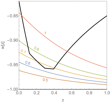
The predictions of $w(z)$ for a given $\lambda$ depend in general on the initial conditions. These are fixed by the requirement that $\Omega_{\phi}(z)$ become negligible at $z>1$, as needed for large-scale structure formation. Therefore, in the far past we begin close to the repulsive fixed point $(x,y)=(0,0)$, and start rolling towards the fixed point at $(x,y)=({\lambda}/{\sqrt{6}},\sqrt{1-\lambda^{2}/6})$, such that $\Omega_{\phi}^{0}=0.7$. In figure 1LABEL:sub@fig:a, we plot the $w(z)$ predictions from these trajectories for a range of values of $\lambda$. We compare these predictions with the current $2\sigma$ upper bounds on $w(z)$ for $0<z<1$ (black curve) [26]. The comparison shows that the upper bound on $\lambda$ is $0.6$, somewhat less than unity.

Second, a universal upper bound on $c$ can be derived for general $\lambda(\phi)$. We claim and will shortly prove that the constant $\lambda$ case with $\lambda(\phi)=c$ is the least constrained trajectory. From above, such a trajectory is ruled out if $c$ is bigger than $0.6$. It follows that every possible $\lambda(\phi)$ is ruled out if $c$ is bigger than $0.6$, leading to the bound $c\lesssim 0.6$.

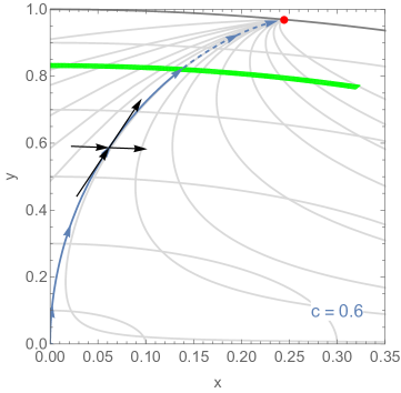
We now provide the argument why the $\lambda(\phi)=c$ trajectory is the limiting case. Figure 1LABEL:sub@fig:b shows in blue the trajectory for the case $\lambda=c=0.6$ which connects the fixed point at $(x,y)=({c}/{\sqrt{6}},\sqrt{1-c^{2}/6})$ to the repulsive fixed point at $(x,y)=(0,0)$. From figure 1LABEL:sub@fig:a, this trajectory fits observational constraints for $0<z<1$ and $z>1$. Where the blue curve intersects the upper black line in the future is the stable fixed point; if the universe began at the repulsive fixed point in the past, the current position along the trajectory is where the blue curve meets the green one.

Note that trajectories are bounded by the condition

$$-\frac{x}{y}<\frac{dy}{dx}<-\frac{x}{y}\left(1-\frac{(1-x^{2}-y^{2})(y^{2}-x^{2})}{\sqrt{\frac{2}{3}}cxy^{2}-x^{2}(1-x^{2}+y^{2})}\right)$$ (13)

where we use the fact that the slope $dy/dx$ for each trajectory at each point is a monotonic function of $\lambda$. Starting from any point in the $x-y$ plot, we can use this condition to bound any trajectory that passes through that point if $\lambda(\phi)>c$. Namely, draw trajectories through the point with $\lambda(\phi)=c$ and $\lambda(\phi)\rightarrow\infty$; these form a cone through which any other trajectory for general $\lambda(\phi)$ must pass. This is illustrated, for example, by the black lines with arrows in Fig.1LABEL:sub@fig:b and the grid of gray lines. Since the blue curve is along one of the edges of this cone, it follows that any trajectory that passes through a point on the right side of the blue curve will stay to the right and cannot cross to its left in the future. Points to the right of the blue curve correspond to larger values of $w(z)$ (equation (9)), and hence all trajectories that are in this region are more constrained by data as shown in figure 1LABEL:sub@fig:a.

Similarly, starting from any point to the left of the blue curve and extrapolating to the past, the trajectory must remain to the left of the blue curve. These trajectories will intersect the $y$-axis at some finite value of $y$ at some finite earlier time. On the $y$-axis, the kinetic energy density is zero, corresponding to a “turning point”. On this trajectory, the field is initially rolling uphill ($x<0$); it stops at the turning point ($x=0$, where the trajectory hits the $y$-axis); and then rolls down hill ($x>0$). The kinetic energy density increases $\propto 1/a^{6}$ compared to matter $\propto 1/a^{3}$ or radiation $\propto 1/a^{4}$ as $a\rightarrow 0$ going back in time. Consequently, the kinetic energy density rapidly grows to dominate over all forms of energy the further back one extrapolates. The result is that any trajectory passing through a point on the left of the blue curve in Fig. 1LABEL:sub@fig:b traces back to $(x,y)=(-1,0)$ or $\Omega_{\phi}=1$ in the early universe. This corresponds to a kinetic energy rather than matter-dominated universe, a trajectory that disrupts large-scale structure formation, and hence is not allowed.

Therefore, we have shown that the blue curve in Fig. 1LABEL:sub@fig:b is the least constrained viable trajectory. As argued above, this leads to the constraint $c\lesssim 0.6$.

One might argue that the point $x=y=0$ is repulsive, so that the initial condition for the $\lambda=c=0.6$ trajectory is fine-tuned. However, it can be realized without fine-tuning in a model with varying $\lambda$. As a simple example, consider a potential with two exponential terms

$$V(\phi) =V_{1}e^{\lambda_{1}\phi/M_{pl}}+V_{2}e^{\lambda_{2}\phi/M_{pl}}$$ (14)

such that $\lambda\approx\lambda_{1}\gg\sqrt{3}$ in the early universe and switches to $\lambda\approx\lambda_{2}=c=0.6$ at some recent point in the past. At early times when $\lambda\approx\lambda_{1}\gg 1$, $\phi$ rolls downhill quickly converging to a scaling solution in which $\Omega_{\phi}\approx 3/\lambda_{1}^{2}\ll 1$, or $(x,y)\approx(0,0)$. At late times when $\lambda\approx\lambda_{2}=c$, the solution flows to dark energy domination and $(x,y)\rightarrow(c/\sqrt{6},\sqrt{1-c^{2}/6})$. Together, these two stages approximate the boundary trajectory. The two exponential model was studied in detail in [29].

The experimental bound we have found for single exponential potential with constant $\lambda$ agrees reasonably with the analysis in [29] based on older data. A good analytical approximation for the limiting trajectory can be found,

$$x \approx\frac{c}{\sqrt{6}}\left(1-\frac{1-\Omega}{\sqrt{\Omega}}\tanh^{-1}(\sqrt{\Omega})\right)\sim\frac{2}{3}\frac{c\,\Omega}{\sqrt{6}}$$ (15)

where in the last term we have used a first order approximation that will be more convenient. This gives a lower bound on $1+w$ for today:

$$1+w(z=0)\gtrsim\frac{4}{27}c^{2}\Omega_{\phi}^{0}$$ (16)

The above derivation assumes that the net field excursion in $\phi$ up until the present is less than $\Delta$, the maximum allowed by Criterion 1. Indeed for the limiting exponential potential we find

$$\Delta\phi=\sqrt{6}\int xdN\simeq\frac{1}{3}c\,{\Omega_{\phi}^{0}}$$ (17)

Interestingly, this provides an observational restriction on the Swampland criterion, namely,

$$\Delta\gtrsim\frac{1}{3}c\ \Omega_{\phi}^{0}\ .$$ (18)

4 Future

The Swampland criteria proposed above also have implications for the possible futures of our universe given current observational constraints on the dark energy density and the equation of state. The bound derived on the slope of the trajectory in equation (13) implies that the value of $x=\dot{\phi}/\sqrt{6}H$ increases in the immediate future.

There are three possible future fates for the universe:

If $\lambda(\phi)$ stays below $\sqrt{3}$, $x$ increases approaching the value $\lambda/\sqrt{6}$. Since the field keeps rolling, Criterion 1 is violated after a finite time. This would imply a breakdown of the effective field theory. The universe would enter a new phase in which a large number of previously massive states become light. This happens when,

$$\Delta\phi=\sqrt{6}\int xdN=\Delta\;{\rm or}\;N<\frac{\Delta}{\sqrt{6}x(N=0)}$$ (19)

$$\Rightarrow N\lesssim\frac{3\Delta}{2c\ \Omega_{\phi}^{0}}$$ (20)

where $N$ is the number of e-foldings. In other words, the new phase would begin within a few Hubble times into the future.

Alternatively, a contrived possibility is that $\lambda(\phi)$ grows very rapidly in the very near future before $\phi$ rolls significantly further downhill. In this case, the universe enters a new phase in which the field speeds up and $w$ grows, ending the cosmic acceleration phase ($w<-\frac{1}{3}$) before $N\sim\frac{3\Delta}{2c\Omega_{\phi}^{0}}$ $e$-folds have passed.

Finally, we can imagine a situation where the potential reaches zero or a negative value before $N\sim\frac{3\Delta}{2c\Omega_{\phi}^{0}}$ $e$-folds have passed. This clearly marks a different kind of new phase of the universe in which supersymmetry might be restored or the universe might enter a phase of contraction.

Here we have enumerated the possible long-term futures of our universe given current observational and theoretical constraints. The fact that in all scenarios the universe survives in its current state at most for a time period of ${\cal O}(1)$ $e$-fold is a novel explanation for the observed age of the universe being of order the current Hubble time. The bound on $N$ implies there is a maximal age to the universe as we know it. The indicator that the end of the current phase is near is signaled by the onset of cosmic acceleration as we have already witnessed in our universe. Observers cannot exist in a universe where dark energy dominates for a long time because the universe changes character first. A typical observer would measure an age comparable to the lifetime of the universe today based on the Swampland analysis.

5 The Role of Observations

The Swampland criteria are based on experience to date in finding constructions that are consistent with a quantum theory of gravity. These suggest a maximal field excursion $\Delta\sim{\cal O}(1)$ and minimum logarithmic slope $|\nabla_{\phi}V|/V>c\sim{\cal O}(1)$. The “$\sim$” in these conditions indicates there is some looseness, although notably there do not exist rigorously proven examples in hand where $c$ is as small as 0.6, as required to satisfy current observational constraints on dark energy. This is exciting because it means that experiments are already sensitive enough to put pressure on string theory and the Swampland.

Based on what we already know observationally about dark energy and what is shown here, there are clearly important challenges for theorists: find rigorous constructions with $c\leq 0.6$ that are consistent with quantum gravity and not in the Swampland (for example, see [30, 31, 32, 33, 34, 35, 36] for an attempt to embed quintessence in string theory). For inflation, not only the bounds on $\{c,\Delta\}$ are somewhat in tension with them being ${\cal O}(1)$ but also almost all current inflationary models studied in the literature have $|\nabla_{\phi}V|/V\rightarrow 0$ at one or more values of $\phi$.

The situation also provides an opportunity for observers and experimentalists: improving bounds on the dark energy equation of state, $w(z)$ for $0<z<1$ could push the limit on $c$ down significantly, further increasing the tension between observations and Criterion 2. Similarly, improved constraints on the tensor-to-scalar ratio $r$ based on CMB observations will add to the tension between inflationary models and the Swampland criteria, perhaps pointing to other theories to explain the large-scale properties of the universe consistent with quantum gravity. Finally, we have motivated the possibility of a direct coupling of the quintessence dark energy field $\phi$ to dark matter. Since the quintessence field is rolling today, and perhaps picking up speed, it is worth searching for evidence that the properties of dark matter (mass, couplings, etc.) are changing e.g. by looking for apparent violations of the equivalence principle in the dark sector.

6 The Cosmological Constant Problem and Quintessence

So far, we have studied what the observational implications of the Swampland criterion are. It is also worth commenting on how these criteria change our perspective on the cosmological constant problem and quintessence. If there are no de Sitter vacua, then the cosmological constant problem takes on a different character.

We can parametrize the scalar potential for $V>0$ without loss of generality as

$$V(\phi) =V_{0}\exp\left(-\int_{0}^{\phi}\frac{d\phi^{\prime}}{M(\phi^{\prime})}\right)$$ (21)

such that $|M_{pl}\nabla_{\phi}V/V|\equiv M_{pl}/M(\phi)$, where we have restored explicit factors of $M_{pl}$ for illustration. Then, assuming that the initial value of the potential is ${\cal{O}}(M_{pl}^{4})$, we find that

$$\int_{0}^{\phi}\frac{d\phi^{\prime}}{M(\phi^{\prime})}=\Delta\phi\left\langle{\frac{1}{M(\phi)}}\right\rangle=\log\frac{\Lambda}{M_{pl}^{4}}\simeq 280$$ (22)

where $\Lambda=(2\ \rm{meV})^{4}$ is the value of the dark energy today. We see that for field excursions of $\mathcal{O}(M_{pl})$, we need $\langle M(\phi)\rangle\sim 10^{-2}M_{pl}$. Therefore, even though $|M_{pl}\nabla_{\phi}V/V|<0.6$ today, it should have been larger in the earlier universe.

Intriguingly, $\langle M(\phi)\rangle\sim 10^{-2}M_{pl}$ points to an interesting scale, the GUT scale. While $M(\phi)$ is a scale in the dark sector, it may be related to $M_{GUT}$ naturally as they are both set by the geometry of the string compactification. This then leads to an expectation for dark energy today of the form

$$\Lambda =M_{pl}^{4}\exp\left(-\frac{\#M_{pl}}{M_{GUT}}\right)$$ (23)

with $\#$ denoting the uncertainty in the field excursion up to the present, expected to be $\mathcal{O}(1)$ in Planck units. Thus, this line of reasoning leads to a relation between the cosmological constant and the GUT scale.

Acknowledgments: We would like to thank R. Daly, A. Ijjas, H. Ooguri, L. Spodyneiko and C. Stubbs for valuable discussions. PA would like to thank the Kavli Institute for Theoretical Physics for their hospitality during the completion of this work. The work of PA is supported by the NSF grants PHY-0855591 and PHY-1216270. PJS thanks the NYU Center for Cosmology and Particle Physics and the Simons Foundation Origins of the Universe Initiative for support during his leave at NYU. PJS is supported by the DOE grant number DEFG02-91ER40671. The work of CV is supported in part by NSF grant PHY-1067976.

References

- [1] C. Vafa, “The String landscape and the swampland,” arXiv:hep-th/0509212 [hep-th].
- [2] T. D. Brennan, F. Carta, and C. Vafa, “The String Landscape, the Swampland, and the Missing Corner,” arXiv:1711.00864 [hep-th].
- [3] H. Ooguri and C. Vafa, “On the Geometry of the String Landscape and the Swampland,” Nucl. Phys. B766 (2007) 21–33, arXiv:hep-th/0605264 [hep-th].
- [4] T. W. Grimm, E. Palti, and I. Valenzuela, “Infinite Distances in Field Space and Massless Towers of States,” arXiv:1802.08264 [hep-th].
- [5] B. Heidenreich, M. Reece, and T. Rudelius, “Emergence and the Swampland Conjectures,” arXiv:1802.08698 [hep-th].
- [6] R. Blumenhagen, “Large Field Inflation/Quintessence and the Refined Swampland Distance Conjecture,” in 17th Hellenic School and Workshops on Elementary Particle Physics and Gravity (CORFU2017) Corfu, Greece, September 2-28, 2017. 2018. arXiv:1804.10504 [hep-th].
- [7] G. Obied, H. Ooguri, L. Spodyneiko, and C. Vafa, “De Sitter Space and the Swampland,” arXiv:1806.08362 [hep-th].
- [8] R. R. Caldwell, R. Dave, and P. J. Steinhardt, “Cosmological imprint of an energy component with general equation of state,” Phys. Rev. Lett. 80 (1998) 1582–1585, arXiv:astro-ph/9708069 [astro-ph].
- [9] A. H. Guth, “The Inflationary Universe: A Possible Solution to the Horizon and Flatness Problems,” Phys. Rev. D23 (1981) 347–356.
- [10] A. D. Linde, “A New Inflationary Universe Scenario: A Possible Solution of the Horizon, Flatness, Homogeneity, Isotropy and Primordial Monopole Problems,” Phys. Lett. 108B (1982) 389–393.
- [11] A. Albrecht and P. J. Steinhardt, “Cosmology for Grand Unified Theories with Radiatively Induced Symmetry Breaking,” Phys. Rev. Lett. 48 (1982) 1220–1223.
- [12] T. Banks, M. Dine, P. J. Fox, and E. Gorbatov, “On the possibility of large axion decay constants,” JCAP 0306 (2003) 001, arXiv:hep-th/0303252 [hep-th].
- [13] N. Arkani-Hamed, L. Motl, A. Nicolis, and C. Vafa, “The String landscape, black holes and gravity as the weakest force,” JHEP 06 (2007) 060, arXiv:hep-th/0601001 [hep-th].
- [14] E. Silverstein and A. Westphal, “Monodromy in the CMB: Gravity Waves and String Inflation,” Phys. Rev. D78 (2008) 106003, arXiv:0803.3085 [hep-th].
- [15] B. Heidenreich, M. Reece, and T. Rudelius, “Weak Gravity Strongly Constrains Large-Field Axion Inflation,” JHEP 12 (2015) 108, arXiv:1506.03447 [hep-th].
- [16] J. Garcia-Bellido, D. Roest, M. Scalisi, and I. Zavala, “Lyth bound of inflation with a tilt,” Phys. Rev. D90 no. 12, (2014) 123539, arXiv:1408.6839 [hep-th].
- [17] BICEP2, Keck Array Collaboration, P. A. R. Ade et al., “Improved Constraints on Cosmology and Foregrounds from BICEP2 and Keck Array Cosmic Microwave Background Data with Inclusion of 95 GHz Band,” Phys. Rev. Lett. 116 (2016) 031302, arXiv:1510.09217 [astro-ph.CO].
- [18] A. Ijjas, P. J. Steinhardt, and A. Loeb, “Inflationary paradigm in trouble after Planck2013,” Phys. Lett. B723 (2013) 261–266, arXiv:1304.2785 [astro-ph.CO].
- [19] E. Silverstein and D. Tong, “Scalar speed limits and cosmology: Acceleration from D-cceleration,” Phys. Rev. D70 (2004) 103505, arXiv:hep-th/0310221 [hep-th].
- [20] F. L. Bezrukov and M. Shaposhnikov, “The Standard Model Higgs boson as the inflaton,” Phys. Lett. B659 (2008) 703–706, arXiv:0710.3755 [hep-th].
- [21] A. A. Starobinsky, “A New Type of Isotropic Cosmological Models Without Singularity,” Phys. Lett. B91 (1980) 99–102. [,771(1980)].
- [22] B. J. Broy, M. Galante, D. Roest, and A. Westphal, “Pole inflation — Shift symmetry and universal corrections,” JHEP 12 (2015) 149, arXiv:1507.02277 [hep-th].
- [23] R. Kallosh and A. Linde, “Universality Class in Conformal Inflation,” JCAP 1307 (2013) 002, arXiv:1306.5220 [hep-th].
- [24] S. Dimopoulos, S. Kachru, J. McGreevy, and J. G. Wacker, “N-flation,” JCAP 0808 (2008) 003, arXiv:hep-th/0507205 [hep-th].
- [25] C. J. A. P. Martins, “The status of varying constants: a review of the physics, searches and implications,” arXiv:1709.02923 [astro-ph.CO].
- [26] D. M. Scolnic et al., “The Complete Light-curve Sample of Spectroscopically Confirmed Type Ia Supernovae from Pan-STARRS1 and Cosmological Constraints from The Combined Pantheon Sample,” arXiv:1710.00845 [astro-ph.CO].
- [27] Planck Collaboration, P. A. R. Ade et al., “Planck 2015 results. XIII. Cosmological parameters,” Astron. Astrophys. 594 (2016) A13, arXiv:1502.01589 [astro-ph.CO].
- [28] S. Tsujikawa, “Quintessence: A Review,” Class. Quant. Grav. 30 (2013) 214003, arXiv:1304.1961 [gr-qc].
- [29] T. Chiba, A. De Felice, and S. Tsujikawa, “Observational constraints on quintessence: thawing, tracker, and scaling models,” Phys. Rev. D87 no. 8, (2013) 083505, arXiv:1210.3859 [astro-ph.CO].
- [30] M. Cicoli, F. G. Pedro, and G. Tasinato, “Natural Quintessence in String Theory,” JCAP 1207 (2012) 044, arXiv:1203.6655 [hep-th].
- [31] G. Gupta, S. Panda, and A. A. Sen, “Observational Constraints on Axions as Quintessence in String Theory,” Phys. Rev. D85 (2012) 023501, arXiv:1108.1322 [astro-ph.CO].
- [32] S. Panda, Y. Sumitomo, and S. P. Trivedi, “Axions as Quintessence in String Theory,” Phys. Rev. D83 (2011) 083506, arXiv:1011.5877 [hep-th].
- [33] N. Kaloper, “Cosmological horizons, quintessence and string theory,” Prog. Theor. Phys. Suppl. 148 (2003) 158–164.
- [34] S. Hellerman, N. Kaloper, and L. Susskind, “String theory and quintessence,” JHEP 06 (2001) 003, arXiv:hep-th/0104180 [hep-th].
- [35] K. Choi, “Quintessence, flat potential and string / M theory axion,” in Supersymmetry, supergravity and superstring. Proceedings, KIAS-CTP International Symposium, Seoul, Korea, June 23-26, 1999, pp. 280–299. 1999. arXiv:hep-ph/9912218 [hep-ph].
- [36] K. Choi, “String or M theory axion as a quintessence,” Phys. Rev. D62 (2000) 043509, arXiv:hep-ph/9902292 [hep-ph].