Calogero-Sutherland Approach to Defect Blocks

Abstract

Extended objects such as line or surface operators, interfaces or boundaries play an important role in conformal field theory. Here we propose a systematic approach to the relevant conformal blocks which are argued to coincide with the wave functions of an integrable multi-particle Calogero-Sutherland problem. This generalizes a recent observation in Isachenkov:2016gim and makes extensive mathematical results from the modern theory of multi-variable hypergeometric functions available for studies of conformal defects. Applications range from several new relations with scalar four-point blocks to a Euclidean inversion formula for defect correlators.

1 Introduction

Extended objects such as line or surface operators, defects, interfaces, and boundaries are important probes of the dynamics in quantum field theory. They give rise to observables that can detect a wide range of phenomena including phase transitions and non-perturbative dualities. In two-dimensional conformal field theories they also turned out to play a vital role for modern formulations of the bootstrap programme. In fact, in the presence of extended objects the usual crossing symmetry becomes part of a much larger system of sewing constraints Cardy:1991tv . While initially the two-dimensional bootstrap started from the crossing symmetry of bulk four-point functions to gradually bootstrap correlators involving extended objects, better strategies were adopted later which depart from some of the sewing constraints involving extended objects. The usual crossing symmetry constraint is then solved at a later stage to find the bulk spectrum and operator product expansion, see e.g. Runkel:2005qw .

The bootstrap programme, whether in its original formulation Polyakov:1974gs , or in the presence of extended objects, relies on conformal partial wave expansions Mack:1973cwx ; Ferrara:1973vz that decompose physical correlation functions into kinematically determined blocks/partial waves and dynamically determined coefficients. These conformal blocks for a four-point correlator are functions of two cross-ratios and the coefficients are those that appear in the operator product expansion of local fields. Such conformal partial wave expansions thereby separate very neatly the dynamical meat of a conformal field theory from its kinematical bones.

In order to perform a conformal block expansion one needs a good understanding of the relevant conformal blocks. While they are in principle determined by conformal symmetry alone, it is still a highly non-trivial challenge to identify them in the zoo of special functions. In the case of scalar four-point functions much progress has been made in the conformal field theory literature starting with Dolan:2000ut ; Dolan:2003hv ; Dolan:2011dv . If the dimension $d$ is even, one can actually construct the conformal blocks from products of two hypergeometric functions each of which depends on one of the cross-ratios. For more generic dimensions many important properties of the scalar blocks have been understood, these include their detailed analytical structure and various series expansions Pappadopulo:2012jk ; Hogervorst:2013sma ; Hogervorst:2013kva ; Isachenkov:2017qgn .

Extended objects give rise to new families of blocks. Previous work on this subject has focused mostly on local operators in the presence of a defect. This includes correlators and blocks for boundary or defect conformal field theory McAvity:1995zd ; Billo:2016cpy ; Lauria:2017wav ; Liendo:2016ymz ; Guha:2018snh , and also bootstrap studies using a combination of numerical an analytical techniques Gaiotto:2013nva ; Liendo:2012hy ; Gliozzi:2015qsa ; Gliozzi:2016cmg ; Lemos:2017vnx ; Liendo:2018ukf . Even in this relatively simple context that involves no more than two cross-ratios, the relevant conformal blocks were only identified in some special cases. More general situations, such as e.g. the correlation function of two (Wilson- or ’t Hooft) line operators in a $d$-dimensional conformal field theory, often possess more than two conformal invariant cross-ratios. Two conformal line operators in a four-dimensional theory, for example, give rise to three cross-ratios. For a configuration of a $p$- and a $q$-dimensional object in a $d$-dimensional theory, the number of cross-ratios is given by $N=\textit{min\/}(d-p,q+2)$ if $p\geq q$ Gadde:2016fbj . So clearly, the study of such defect correlation functions involves new types of special functions which depend on more than two variables.

In order to explore the features of these new functions, understand their analytical properties or find useful expansions one could try to follow the same route that was used for four-point blocks, see e.g. Fukuda:2017cup ; Kobayashi:2018okw for some recent work in this direction. It is the central message of this paper, however, that there is another route that gives a much more direct access to defect blocks. It relies on a generalization of an observation in Isachenkov:2016gim that four-point blocks are wave functions of certain integrable two-particle Hamiltonians of Calogero-Sutherland type Calogero:1970nt ; Sutherland:1971ks . The solution theory for this quantum mechanics problem is an important subject of modern mathematics, starting with the seminal work of Heckman-Opdam Heckman:1987 , see Isachenkov:2017qgn for a recent review in the context of conformal blocks. Much of the development in mathematics is not restricted to the two-particle case and it has given rise to an extensive branch of the modern theory of multi-variable hypergeometric functions.

In order to put all this mathematical knowledge to use in the context of defect blocks, all that is missing is the link between the corresponding conformal blocks, which depend on $N$ variables, to the wave functions of an $N$-particle Calogero-Sutherland model. Establishing this link is the main goal of our paper. Following a general route through harmonic analysis on the conformal group that was proposed in Schomerus:2016epl , we construct the relevant Calogero-Sutherland Hamiltonian, i.e. we determine the parameters of the potential in terms of the dimensions $p,q$ of the defects and the dimension $d$. In the special case of correlations of bulk fields in the presence of a defect, the parameters also depend on the conformal weights of the external fields. All these results will be stated in section 3 along with a sketch of the proof.

Calogero-Sutherland models possess a number of fundamental symmetries that can be composed to produce an exhaustive list of relations between defect blocks. We will present these as a first application of our approach in section 3.2. Special attention will be paid to relations involving scalar four-point blocks for which we produce a complete list that significantly extends previously known constructions of defect blocks.

As interesting as such relations are, they provide only limited access to defect blocks. We develop the complete solution theory for defect blocks with $N=2$ and $N>2$ cross-ratios in section 4 and 5 by exploiting known mathematical results on the solutions of Calogero-Sutherland eigenvalue equations. A lightning review of the mathematical input is included in section 4, following Isachenkov:2017qgn . In particular, we shall review the concept of Harish-Chandra scattering states, discuss the issue of series expansions, poles and their residues, as well as global analytical properties such as cuts and their monodromies. In the final section we put all these results together to construct defect conformal partial waves and blocks. By definition, the former are linear combinations of conformal blocks that are single valued in the Euclidean domain and feature in the Euclidean inversion formula. The paper concludes with an outlook and a list of important open problems.

2 Setup and review of previous results

Before we begin discussing our new Calogero-Sutherland approach to defect blocks, we want to summarize the main results that are present in the existing conformal field theory literature. The setup that has received most attention involves two bulk fields in the presence of a $p$-dimensional defect. For such correlators, the conformal blocks are known at least as series expansions Billo:2016cpy ; Lauria:2017wav or, more explicitly, through relations with scalar four-point blocks which exist for some special cases, see subsection 2.3. Results on conformal blocks in the more generic setup when none of the defects is point-like are particularly scarce, see however Gadde:2016fbj , where the number of independent cross-ratios was counted and a particular set of cross-ratios was constructed. We shall review some key ingredients from Gadde:2016fbj in subsection 2.2. This subsection also contains a parametrization of defect cross-ratios in terms of new geometric variables that will turn out to be particularly well adapted to our Calogero-Sutherland models later on.

2.1 Two-point functions in defect CFT

In order to describe existing results concerning two bulk fields in the presence of a defect (or boundary), we briefly review the embedding formalism, which is a standard approach frequently used to study correlators in conformal field theory. For details on the embedding space formalism see for example Costa:2011mg . The adaptation to the defect setup can be found in Billo:2016cpy ; Gadde:2016fbj , see also the next subsection.

Because the Euclidean conformal group in $d$ dimensions is $\mathrm{SO}{(1,d+1)}$ it is natural to represent its action linearly on an embedding space $\mathbb{R}^{1,d+1}$. In order to retrieve the usual non-linear action of the conformal group on the $d$-dimensional Euclidean space we must get rid of the two extra dimensions. This is done by restricting the coordinates to the projective null cone, i.e. we demand $X^{2}=0$ for $X\in\mathbb{R}^{1,d+1}$ and identify $X\sim gX$ for $g\in\mathbb{R}$. It is useful to work in lightcone coordinates with dot product given by

$$X\cdot Y=(X^{+},X^{-},X^{i})\cdot(Y^{+},Y^{-},Y^{i})=-\frac{1}{2}(X^{+}Y^{-}+X^{-}Y^{+})+X^{i}Y^{i}\,.$$ (1)

In other words, points on the physical space $x\in\mathbb{R}^{d}$ are represented by elements of the projective lightcone of the embedding space. It is common to use the projective identification $X\sim gX$ in order to fix a particular section of the cone given by

$$X=(1,x^{2},x^{\mu})\,.$$ (2)

This is called the Poincaré section. Note that this section is invariant under $\mathrm{SO}{(1,d+1)}$ only up to projective identifications. The point at infinity is lifted to $\Omega=(0,1,0^{\mu})$.

Extended operators or defects in conformal field theories do not preserve the $\mathrm{SO}{(1,d+1)}$ symmetry of the conformal group. However, if we consider a $p$-dimensional conformal defect its support is left invariant by the subgroup $\mathrm{SO}{(1,p+1)}\times\mathrm{SO}{(d-p)}\subset\mathrm{SO}{(1,d+1)}$. Indices that transform non-trivially under the first factor $\mathrm{SO}{(1,p+1)}$ will be denoted by $A,B,\dots$ while those that transform non-trivially under the rotation group $\mathrm{SO}{(d-p)}$ will be denoted by $I,J,\dots$, i.e. we split $X\in\mathbb{R}^{1,d+1}$ as

$$(X^{A})=(X^{0},X^{1},\ldots,X^{p+1})\,,\qquad(X^{I})=(X^{p+2},\ldots,X^{d+1})\,,$$ (3)

into components along and transverse to the defect. With these introductory remarks on the embedding space, we are now prepared to discuss two-point functions.

Let us represent the insertion points of the two bulk fields by $X_{1}$ and $X_{2}$. Since the $p$-dimensional defect splits the $d$-dimensional conformal group into two factors, see previous paragraph, it is natural to introduce the following product

$$X_{1}\circ X_{2}=X_{1}^{I}\delta_{IJ}X_{2}^{J}\,.$$ (4)

Here, summation over the transverse indices $I,J=p+2,\dots,d+1$ is understood. We can now choose two conformal invariants

$$\frac{(1-x)(1-\bar{x})}{(x\bar{x})^{\frac{1}{2}}}=-\frac{2X_{1}\cdot X_{2}}{(X_{1}\circ X_{1})^{\frac{1}{2}}(X_{2}\circ X_{2})^{\frac{1}{2}}}\,,\qquad\frac{x+\bar{x}}{2(x\bar{x})^{\frac{1}{2}}}=\frac{X_{1}\circ X_{2}}{(X_{1}\circ X_{1})^{\frac{1}{2}}(X_{2}\circ X_{2})^{\frac{1}{2}}}\,.$$ (5)

The choice of cross-ratios $(x,\bar{x})$ may not appear to be the most natural one at first, but they turn out have a clean interpretation in terms of coordinates in a plane orthogonal to the defect, see figure 1. Conformal symmetry constrains two-point functions to be of the form

$$\langle O_{1}(X_{1})O_{2}(X_{2})\rangle^{(p)}_{\textit{defect}}=\frac{\mathcal{F}(x,\bar{x})}{(X_{1}\circ X_{1})^{\tfrac{\Delta_{1}}{2}}(X_{2}\circ X_{2})^{\tfrac{\Delta_{2}}{2}}}\,,$$ (6)

where the function $\mathcal{F}(x,\bar{x})$ has two conformal block expansions: the bulk channel and the defect channel to be described below.

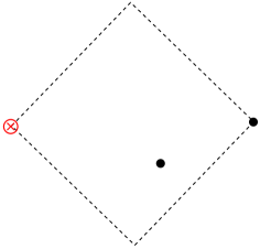
Figure 1: Two-point function configuration in a plane orthogonal to the defect. The defect is at the origin while the operators $O_{1}$ and $O_{2}$ are at points $(1,1)$ and $(x,\bar{x})$, respectively.

2.1.1 Bulk channel conformal blocks

The bulk channel expansion is obtained by using the standard operator product expansion for two local bulk fields before evaluating the one-point functions of the resulting bulk fields in the background of the defect,

$$\mathcal{F}(x,\bar{x})=\left(\frac{(1-x)(1-\bar{x})}{(x\bar{x})^{\frac{1}{2}}}\right)^{-\frac{\Delta_{1}+\Delta_{2}}{2}}\sum_{k}c_{12k}C^{\mathcal{D}}_{k}\mathop{f}\left(\begin{matrix}p,a,d\\ \Delta_{k},\ell_{k}\end{matrix};x,\bar{x}\right)\,,$$ (7)

where we made the dependence on the defect dimension $p$, the relevant information about the external scalars $a=(\Delta_{2}-\Delta_{1})/2$, and the dimension $d$ explicit.

The conformal field theory data in this channel corresponds to the bulk three-point coupling $c_{12k}$ multiplied with the coefficients $C^{\mathcal{D}}_{k}$ of the one-point function of scalar operators. The general form of the bulk channel blocks cannot be found in closed-form in the existing literature, see however Lauria:2017wav for efficient power series expansions. For some selected cases the defect block can be mapped to the conformal blocks for four scalars in standard bulk conformal field theory, see sections 2.3 and 3.2 below and appendix B. Our results in sections 4-5 generalize these isolated results and thereby fill an important gap.

2.1.2 Defect channel conformal blocks

Local operators in the bulk of a defect conformal field theory may be expanded in terms of operators that are inserted along the defect. We will denote such operators by $\hat{O}$ and the associated operator product coefficients for the bulk fields $O_{i},i=1,2$ through $b_{i\hat{O}}$. Applying such a defect expansion to the external operators results in the following conformal block expansion

$$\mathcal{F}(x,\bar{x})=\sum_{k}b_{1k}b_{2k}\hat{f}_{\widehat{\Delta}_{k},s_{k}}(x,\bar{x})\,,$$ (8)

where $k$ runs through the set of all intermediate fields $\widehat{O}=\widehat{O}_{k}$ of weight $\widehat{\Delta}_{k}$ and spin $s_{k}$. The blocks $\hat{f}(x,\bar{x})$ factorize in terms of the $\mathrm{SO}{(d-1,1)}\times\mathrm{SO}{(d-p)}$ symmetry group. This simplifies the analysis significantly and it is possible to write $\hat{f}(x,\bar{x})$ as a product of hypergeometric functions

$$\hat{f}_{\widehat{\Delta},s}(x,\bar{x})=x^{\frac{\widehat{\Delta}-s}{2}}\bar{x}^{\frac{\widehat{\Delta}+s}{2}}{}_{2}F_{1}\left(-s,\frac{d-p}{2}-1,2-\frac{d-p}{2}-s,\frac{x}{\bar{x}}\right){}_{2}F_{1}\left(\widehat{\Delta},\frac{p}{2},\widehat{\Delta}+1-\frac{p}{2},x\bar{x}\right)\,.$$

In the following we shall mostly focus on the bulk channel and its generalizations. A few more comments on the defect channel and its role in the bootstrap can be found in the concluding section.

Boundary CFT.

As an aside let us comment on the boundary case which is special, since the transverse space is one-dimensional ($p=d-1$). In this case the two-point function depends only on the first invariant in eq. (5)

$$\langle O_{1}(X_{1})O_{2}(X_{2})\rangle_{\textit{BCFT}}=\frac{1}{(X_{1}\circ X_{1})^{\tfrac{\Delta_{1}}{2}}(X_{2}\circ X_{2})^{\tfrac{\Delta_{2}}{2}}}f\left(\frac{(1-x)(1-\bar{x})}{(x\bar{x})^{\frac{1}{2}}}\right)\,.$$ (9)

The conformal block expansion of this correlator was originally studied in McAvity:1995zd , and the boundary bootstrap was implemented in Liendo:2012hy ; Gliozzi:2015qsa ; Gliozzi:2016cmg .

2.2 Cross-ratios for two conformal defects

While some of our new results do concern the configurations considered in the previous subsection, our approach covers a more general setup involving two defects of dimension $p$ and $q$, respectively. The first systematic discussion of such defect correlators can be found in Gadde:2016fbj . That paper determined the number $N$ of cross-ratios and also introduced a particular set of coordinates on the space of these cross-ratios. Here we shall review the latter before we discuss an alternative, and more geometric choice of coordinates.

As we have discussed already, a $p+2$-dimensional hyperplane in $\mathbb{R}^{1,d+1}$ with a time-like direction preserves the subgroup $\mathrm{SO}{(1,p+1)}\times\mathrm{SO}{(d-p)}$ of the conformal group. Furthermore, it can be shown that the intersection of such a hyperplane with the Poincaré section projects down to a $p$-sphere in $\mathbb{R}^{d}$ Gadde:2016fbj , the locus of the defect in Euclidean space. Hence, one can parametrize the position of the defect through $(d-p)$ orthonormal vectors $P_{\alpha},\alpha=1,\dots,d-p$, one for each transverse direction. In order to do so, we first pick any $p+2$ points $x_{k}$, $k=1,\dots,p+2$, on the defect $\mathcal{D}^{(p)}\subset\mathbb{R}^{d}$ and consider their lift $X_{k}=(1,x_{k}^{2},x_{k})$ to the Poincaré section. This uniquely defines the $(p+2)$-dimensional hyperplane. To select a set of vectors $P_{\alpha}$, which are of course not unique, we demand that $X_{k}\cdot P_{\alpha}=0$ and $P_{\alpha}\cdot P_{\beta}=\delta_{\alpha\beta}$. Besides conformal transformations, there also exists an $\mathrm{O}(d-p)$ gauge symmetry which acts on the index $\alpha$, i.e. it transforms the vectors $P_{\alpha}$ into each other. In order to study the two-point function of two defect operators $\mathcal{D}^{(p)}(P_{\alpha})$ and $\mathcal{D}^{(q)}(Q_{\beta})$ that are inserted along surfaces associated with $P_{\alpha}$ and $Q_{\beta}$, respectively, we need to single out the invariant cross-ratios. Consider the matrix with elements $M_{\alpha\beta}=P_{\alpha}\cdot Q_{\beta}$ of conformal invariants. The residual gauge symmetries $\mathrm{SO}{(d-p)}$ and $\mathrm{SO}{(d-q)}$ which act on the matrix $M$ through left- and right multiplication, respectively, can be used to diagonalize $M$. The non-trivial eigenvalues provide a complete set of independent cross-ratios.

To determine their number we need a bit more detail. First, let us consider the case in which the hyperplanes that are spanned by $P_{\alpha}$ and $Q_{\beta}$ have no directions in common. This requires that $2d-p-q\leq d+2$ or equivalently $d-p\leq q+2$. If we assume $p\geq q$ from now on, the number of cross-ratios is given by $N=d-p$,

$$\begin{matrix}M=\left.\begin{pmatrix}*&*&*&*&*\\ *&*&*&*&*\\ \makebox[0.0pt][l]{$\smash{\underbrace{\phantom{\begin{matrix}*&*&*&*&*\end{matrix}}}_{\text{\scriptsize$d-q$}}}$}*&*&*&*&*\end{pmatrix}\right\}\text{\scriptsize$d-p$}\ \mathop{\xrightarrow{\hskip 56.9055pt}}\limits^{\mathrm{SO}{(d-p)}}_{\mathrm{SO}{(d-q)}}\ \begin{pmatrix}*&0&0&0&0\\ 0&*&0&0&0\\ \makebox[0.0pt][l]{$\smash{\underbrace{\phantom{\begin{matrix}0&0&*\end{matrix}}}_{\text{\scriptsize$d-p$}}}$}0&0&*&0&0\end{pmatrix}\\ \mathstrut\end{matrix}\,.$$ (10)

If $d-p>q+2$, on the other hand, the two hyperplanes spanned by $P_{\alpha}$ and $Q_{\beta}$ must intersect in $d-2-(p+q)$ directions. Hence $d-2-(p+q)$ of the scalar products are invariant and there are only $d-p-(d-2-(p+q))=q+2$ nontrivial eigenvalues,

$$\begin{matrix}M=\left.\begin{pmatrix}*&*&*&*&*\\ *&*&*&*&*\\ \makebox[0.0pt][l]{$\smash{\underbrace{\phantom{\begin{matrix}*&*&*&*&*\end{matrix}}}_{\text{\scriptsize$d-q$}}}$}*&*&*&*&*\end{pmatrix}\right\}\text{\scriptsize$d-p$}\ \mathop{\xrightarrow{\hskip 56.9055pt}}\limits^{\mathrm{SO}{(d-p)}}_{\mathrm{SO}{(d-q)}}\ \begin{pmatrix}*&0&0&0&0\\ 0&*&0&0&0\\ \makebox[0.0pt][l]{$\smash{\underbrace{\phantom{\begin{matrix}0&0\end{matrix}}}_{\text{\scriptsize$q+2$}}}$}0&0&1&0&0\end{pmatrix}\\ \mathstrut\end{matrix}\,.$$ (11)

In total, the number of invariant cross-ratios is therefore $N=\min(d-p,q+2)$. To be precise, we point out that the full gauge group is actually given by $\mathrm{O}(d-p)\times\mathrm{O}(d-q)$ and hence the values on the diagonal are only meaningful up to a sign. One way to construct fully invariant cross-ratios is to consider

$$\eta_{a}=\mathop{tr}(MM^{T})^{a}\,$$ (12)

where $a=1,\dots,N$. This is the set of cross-ratios introduced in Gadde:2016fbj . Here we want to consider a second, alternative set, that is more geometric and also will turn out later to possess a very simple relation with the coordinates of the Calogero-Sutherland Hamiltonian.

Roughly, our new parameters consist of the ratio $R/r$ of radii of the spherical defects along with $N-1$ tilting angles $\theta_{i}$ of the lower $(q-)$dimensional defect in the space that is transverse to the higher $(p-)$dimensional defect. To be more precise, we place our two spherical defects of dimensions $p$ and $q$, respectively, such that they are both centered at the origin $\mathbb{R}^{d}$. Without restriction we can assume that the $p-$dimensional defect of radius $R$ is immersed in the subspace spanned by the first $p+1$ basis vectors $e_{1},\dots,e_{p+1}$ of the $d$-dimensional Euclidean space. The radius of the second, $q-$dimensional defect, we denote by $r$. To begin with, we insert this defect in the subspace spanned by the first $q+1$ basis vectors $e_{1},\dots,e_{q+1}$. Then we tilt the second defect by angles $\theta_{1},\dots,\theta_{N-1}$ in the $e_{1}-e_{d},\dots,e_{N-1}-e_{d+2-N}$ planes, respectively. In other words we act on the locus of the second sphere with 2-dimensional rotation matrices $R_{(i-1,d+2-i)}(\theta_{i})$ in the plane spanned by the basis vectors $e_{i-1}$ and $e_{d+2-i}$ for $i=1,\dots,N-1$. This gives a well-defined configuration of defects, because we have $N-1\leq q+1\leq p+1<d+2-N$ for $p\geq q$. With a little bit of work it is possible to compute the matrix $M$ of scalar products explicitly, see appendix A for a derivation,

$$M=\left(\begin{array}[]{@{}ccccc|c@{}}\cosh\vartheta&&&&&\\ &\cos\theta_{1}&&&&\\ &&\ddots&&&\scalebox{1.5}{0}\\ &&&\cos\theta_{N-1}&&\\ &&&&I&\end{array}\right)\quad\textrm{where}\quad\cosh\vartheta=\frac{1}{2}\left(\frac{r}{R}+\frac{R}{r}\right)\,.$$ (13)

We shall pick $\vartheta$ to be a positive real number. Using the general prescription (12) the cross-ratios $\eta_{a}$ that were introduced in Gadde:2016fbj take the form

$$\eta_{a}=\cosh^{2a}\vartheta+\cos^{2a}\theta_{1}+\dots+\cos^{2a}\theta_{N-1}\,,\quad a=1,\dots,N\,.$$ (14)

From now on we shall adopt the parameters $\vartheta$ and $\theta_{i},i=1,\dots,N-1$ as the fundamental conformal invariants for $N\geq 3$. While $\vartheta$ can be any non-negative real number, the variables $\theta_{i}$ take values in the interval $\theta_{i}\in[0,\pi[$.

Let us stress once again, that our geometric parameters $R/r$ and $\theta_{i}$ represent just one convenient choice. In the special case with $p=q=d-2$, the variables $\eta_{1}$ and $\eta_{2}$ possess a direct geometric interpretation that is based on a slightly different setup in which one defect is assumed to be flat while the second is kept at finite radius but displaced and tilted with respect to the first, see Gadde:2016fbj . Another important special case appears for $q=0$, i.e. when two bulk fields are placed in the background of a defect, which we discussed at length in the previous subsection. In particular, we have introduced a geometric parametrization of the two cross-ratios, namely through the parameters $x$ and $\bar{x}$, see eq. (5). It is not too difficult to work out, see appendix A, that these are related to the parameters $\vartheta$ and $\theta\equiv\theta_{1}$ through

$$x=\tanh^{-2}\frac{\vartheta+i\theta}{2}\,,\quad\bar{x}=\tanh^{-2}\frac{\vartheta-i\theta}{2}\,.$$ (15)

We will use the coordinates $x$, $\bar{x}$ as the fundamental conformal invariants for $N=2$. Eq. (15) also shows that the variables $\vartheta$ and $\theta_{i}$ generalize the radial coordinates that were introduced for $N=2$ in Lauria:2017wav .

2.3 Defect partial wave expansion and blocks

After having identified the variables, we can write down the two-point function of defects $\mathcal{D}^{(p)}(P_{\alpha})$ and $\mathcal{D}^{(q)}(Q_{\beta})$, i.e. generalize eqs. (6) and (7) to an arbitrary pair of defects. Conformal invariance restricts its form to be

$$\langle\mathcal{D}^{(p)}(P_{\alpha})\mathcal{D}^{(q)}(Q_{\beta})\rangle=\sum_{k}C^{\mathcal{D}^{(p)}}_{k}C^{\mathcal{D}^{(q)}}_{k}\mathop{f_{D}}\left(\begin{matrix}p,q,d\\ \Delta_{k},\ell_{k}\end{matrix};\vartheta,\theta_{i}\right)\,,$$ (16)

where the spin $\ell$ is labeled by a set of even integers $\ell=(l_{1},\dots,l_{N-1})$ with $l_{1}\geq\dots\geq l_{N-1}\geq 0$ and the defect blocks $f_{D}$ are normalized such that

$$\mathop{f_{D}}\left(\begin{matrix}p,q,d\\ \Delta,\ell\end{matrix};\vartheta,\theta_{i}\right)\stackrel{{\scriptstyle\vartheta\rightarrow\infty}}{{\rightarrow}}4^{\Delta}e^{-\Delta\vartheta}\prod_{i=1}^{N-1}(-2\cos\theta_{i})^{l_{i}}\,,$$ (17)

so that $C^{\mathcal{D}^{(p)}}_{k}$ are the coefficient in the defect expansion of the defect in terms of local bulk operators

$$\mathcal{D}(P_{\alpha})=\sum_{\Phi}C^{\mathcal{D}}_{\Phi}D_{\Delta_{\Phi}}(P_{\alpha},X,\partial_{X})\Phi(X)\,.$$ (18)

The partial wave expansion (16) separates these dynamical data from the kinematical skeleton of the correlation function. The latter enters through the conformal blocks $f_{D}(\vartheta,\theta_{i})$ which are the main objects of interests for the present work. As we mentioned before, these blocks are known in a few examples where they can be related to the blocks of four scalar bulk fields.

The first example we want to discuss here is taken from Liendo:2016ymz . It applies to the case in which two bulk fields in $d=4$ dimensions are inserted into the background of a line defect, i.e. $p=1$ and $q=0$. In order to relate the defect block $f(x,\bar{x})$ to the blocks $g(\gamma,\bar{\gamma})$ of four scalar fields, let us consider the following change of coordinates

$$\gamma=\left(\frac{1-x}{1+x}\right)^{2}\,,\quad\bar{\gamma}=\left(\frac{1-\bar{x}}{1+\bar{x}}\right)^{2}\,.$$ (19)

which maps the Euclidean region of the defect coordinates $x,\bar{x}$ to the Euclidean region of the four-point cross-ratios $\gamma$, $\bar{\gamma}$. Given this change the following identity holds Liendo:2016ymz

$$\mathop{f}\left(\begin{matrix}1,0,4\\ \Delta,\ell\end{matrix};x,\bar{x}\right)\propto(\gamma\bar{\gamma})^{-\frac{1}{4}}\mathop{g}\left(\begin{matrix}\frac{1}{4},-\frac{1}{4},3\\ \frac{\Delta+1}{2},\frac{\ell}{2}\end{matrix};\gamma,\bar{\gamma}\right)\,.$$ (20)

The lower indices on the block $g$ refer to the conformal weight and spin of the intermediate field. The upper indices $(a,b,d)=(1/4,-1/4,3)$ contain the relevant information about the external scalars, i.e. the parameters $a=(\Delta_{2}-\Delta_{1})/2,b=(\Delta_{3}-\Delta_{4})/2$ and the dimension $d$. Note that the four-point block on the right hand side is the one with $\Delta_{1}-\Delta_{2}=\Delta_{3}-\Delta_{4}=-1/2$ and dimension $d=3$ even though the original defect setup is in $d=4$ dimensions and involves two bulk fields of the same weight.

A second example for a relation between defects and scalar four-point was pointed out in Gadde:2016fbj . Conformal blocks for the two-point function of defects of dimension $p=q=d-2$ can be mapped to the four-point function of scalars with the following relation between the different variables

$$\eta_{1}=\frac{2(1+v)}{u}\,,\quad\eta_{2}=\frac{2(1+6v+v^{2})}{u^{2}}$$ (21)

where $u$ and $v$ are related to the usual cross-ratios $z$ and $\bar{z}$ as $u=z\bar{z}$ and $v=(1-z)(1-\bar{z})$. The relation between $\eta_{a}$ and $\theta_{1},\vartheta$ is given in eq. (14). With this change of variables the relation of Gadde:2016fbj reads

$$\mathop{f_{D}}\left(\begin{matrix}d-2,d-2,d\\ \Delta,\ell\end{matrix};\vartheta,\theta_{1}\right)=\mathop{g}\left(\begin{matrix}0,0,d\\ \Delta,\ell\end{matrix};z,\bar{z}\right)\,.$$ (22)

As in the previous example, the Euclidean region of the defect block is mapped to a pair of complex conjugate variables $z,\bar{z}$ and hence to the Euclidean region of the four-point blocks. The scalar block on the right hand side is the one with $a=b=0$ and the same dimension $d$ as on the left hand side.

Another relation between blocks was proposed in Billo:2016cpy (chronologically this was the first such relation found). These authors considered two bulk fields, i.e. $q=0$, in the presence of a defect of dimension $p=d-2$ and found the following relation between the corresponding defect blocks in the bulk channel with four-point blocks:

$$\mathop{f}\left(\begin{matrix}d-2,0,d\\ \Delta,\ell\end{matrix};x,\bar{x}\right)\sim\mathop{g}\left(\begin{matrix}0,0,d\\ \Delta,\ell\end{matrix};1-x,1-\frac{1}{\bar{x}}\right)\,.$$ (23)

Here we should point out however, that this relation does not map the Euclidean region of the defect block to the Euclidean region of the scalar four-point block. In fact, it maps two Lorentzian regions into each other, see also Lauria:2017wav . Hence, any relation of the form (23) involves an analytic continuation. Since the blocks possess branch cuts, this continuation requires additional choices. In this case, the lightcone OPE implies that the ambiguity is just a global phase, and indeed (23) gives the correct defect block. Nevertheless, the r.h.s. of (23) is not a Euclidean four-point block, but the analytic continuation of such, this is why we put a $\sim$ instead of an equality. We will come back to this issue in section 5.

As we will see, the technology presented in the next section will explain all these relations and vastly generalize them, through a (re-)interpretation as symmetries of Calogero-Sutherland models.

3 Calogero-Sutherland model for Casimir equations

In this section we want to describe a fully systematic framework for the Casimir equations of conformal blocks for correlation functions of two defects. Rather than working with the popular embedding space, we shall realize all blocks as functions on the conformal group itself. If the latter is equipped with an appropriate set of coordinates, the Casimir equations assume a universal form. In fact, they can be phrased as an eigenvalue problem for an $N$-particle Calogero-Sutherland system. We will review the result in the first subsection, discuss some immediate consequences of the equations and their symmetries in the second and sketch the derivation of our results in the third.

3.1 Calogero-Sutherland models for defects

We will show below that the Casimir equations for conformal blocks of two defects can be restated as an eigenvalue problem for the Calogero-Sutherland Hamiltonian of the form

$$H_{\textrm{CS}} =-\sum_{i=1}^{N}\frac{\partial^{2}}{\partial\tau_{i}^{2}}+\frac{k_{3}(k_{3}-1)}{2}\sum_{i<j}^{N}\left[\sinh^{-2}\left(\frac{\tau_{i}+\tau_{j}}{2}\right)+\sinh^{-2}\left(\frac{\tau_{i}-\tau_{j}}{2}\right)\right]$$

$$\qquad+\sum_{i=1}^{N}\left[k_{2}(k_{2}-1)\sinh^{-2}\left(\tau_{i}\right)+\frac{k_{1}(k_{1}+2k_{2}-1)}{4}\sinh^{-2}\left(\frac{\tau_{i}}{2}\right)\right]\ .$$ (24)

The coupling constants $k_{i},i=1,2,3$ that appear in the potential are referred to as multiplicities in the mathematical literature. In principle, these can assume complex values though we will mostly be interested in cases in which they are real. The coordinates $\tau_{i}$ may also be complex in general. Later we will describe their values in more detail. The case $N=1$ is a bit special since it involves only two coupling constants.

The Calogero-Sutherland Hamiltonian possesses two different interpretations. We can think of it as describing a system of $N$ interacting particles that move on a one-dimensional half-line with external potential. The external potential is given by the terms in the second line of eq. (3.1). These terms contains two of the three coupling constants, namely $k_{1}$ and $k_{2}$. The interaction terms, on the other hand, involve the third coupling constant $k_{3}$. Alternatively, we can also think of a scattering problem for a single particle in an $N-$dimensional space. We will mostly adopt the second view below.

Let us note that the multiplicities are not defined uniquely, i.e. different choices of the multiplicities $k_{i}$ can give rise to identical Casimir equations. This is partly due to the fact that the multiplicities appear quadratically in the potential. In addition, one may show that a simultaneous shift of all coordinates $\tau_{i}\rightarrow\tau_{i}+i\pi$ for $i=1,\dots,N$ leads to a Calogero-Sutherland Hamiltonian of the form (3.1) with different multiplicities. The complete list of symmetries is given in table 1. Later we see that these innocent looking replacements have remarkable consequences, since they produce non-trivial relations between the blocks of various (defect) configurations.

Table 1: Symmetries of the Calogero-Sutherland model for generic values of the multiplicities. The last symmetry also involves a shift $\tau^{\prime}_{i}=\tau_{i}\pm i\pi$ of the coordinates.

	$k^{\prime}_{1}$	$k^{\prime}_{2}$	$k^{\prime}_{3}$
$\varrho_{1}$	$1-k_{1}-2k_{2}$	$k_{2}$	$k_{3}$
$\varrho_{2}$	$-k_{1}$	$1-k_{2}$	$k_{3}$
$\varrho_{3}$	$k_{1}$	$k_{2}$	$1-k_{3}$
$\tilde{\varrho}$	$k_{1}$	$1-k_{1}-k_{2}$	$k_{3}$

Let us now describe the main new results of this work. The first case to look at is the case of two defects of dimension $p\geq q$ with $q\neq 0$. The corresponding Casimir equation for conformal blocks is an eigenvalue equation for the operator

$$L^{2}=H_{CS}+\epsilon_{0}\,,\quad\epsilon_{0}=\frac{N}{8}\left(\frac{d(d+2)}{2}-N(d+1)+\frac{2N^{2}+1}{3}\right)$$ (25)

with the following choice of parameters

$$N =\min(d-p,q+2)\,,\quad k_{1}=\frac{d}{2}-(p-q)-N+1\,,\quad k_{2}=\frac{p-q}{2}\,,\quad k_{3}=\frac{1}{2}\,.$$ (26)

Let us note that in a representation of spin $\ell$ and weight $\Delta$, the operator $L^{2}$ assumes the value

$$C_{\Delta,J}=\Delta(\Delta-d)+\sum_{i=1}^{N-1}l_{i}(l_{i}+d-2i)\,,$$ (27)

where the spin $\ell$ is labeled by a set of even integers $\ell=(l_{1},\dots,l_{N-1})$ with $l_{1}\geq\dots\geq l_{N-1}\geq 0$. The wave function $\psi(\tau)$ is given by the Schrödinger-like equation

$$H_{CS}\psi_{\epsilon}(\tau)=\epsilon\psi_{\epsilon}(\tau)$$ (28)

and is related to the conformal block by

$$\mathop{f_{D}}\left(\begin{matrix}p,q,d\\ \Delta,\ell\end{matrix};\tau\right)=2^{2\Delta-\frac{1}{2}N(d-N+1)}\omega(\tau)\psi_{\epsilon}(\tau)\,,\quad\epsilon=-\frac{1}{4}C_{\Delta,\ell}-\epsilon_{0}\,,$$ (29)

where the “gauge transformation” $\omega(\tau)$ is given by

$$\omega(\tau) =\prod_{i=1}^{N}\sinh^{N-\frac{d}{2}+\frac{p-q}{2}-1}\left(\frac{\tau_{i}}{2}\right)\cosh^{-\frac{p-q}{2}}\left(\frac{\tau_{i}}{2}\right)\prod_{i<j}\sinh^{-\frac{1}{2}}\left(\frac{\tau_{i}\pm\tau_{j}}{2}\right).$$ (30)

Here and throughout the entire text below we use the shorthand

$$\sinh\left(\frac{x\pm y}{2}\right)=\sinh\left(\frac{x+y}{2}\right)\sinh\left(\frac{x-y}{2}\right)\,.$$ (31)

Equation (28) is to be considered on a subspace of the semi-infinite hypercuboid $A^{E}_{N}$ that is parametrized by the coordinates

$$\tau_{1}=2\vartheta=2\log\frac{R}{r}\in[0,\infty)\,,\quad\tau_{j+1} =2i\theta_{j}\in i[0,2\pi]\,,$$ (32)

for $j=1,\dots,N-1$. We shall discuss the domain in much more detail in section 5.1. Of course, the choice of multiplicities $k_{i}$ is not unique since we can apply any of the transformations listed in table 1. We will discuss the consequences in the next subsection.

If $q=0$ while $0<p\leq d-2$, the setup describes two scalar bulk fields in the presence of a $p$-dimensional defect of co-dimension greater or equal to two. In this case, the conformal Casimir operator takes the form

$$L^{2}=H_{CS}+\epsilon_{0}\,,\quad\epsilon_{0}=\frac{d^{2}-2d+2}{8}$$ (33)

with parameters

$$N =2\,,\quad k_{1}=\frac{d}{2}-p-1\,,\quad k_{2}=\frac{p}{2}\,,\quad k_{3}=\frac{1}{2}+a\,.$$ (34)

Here, the parameter $a$ is related to the conformal weights $\Delta_{1}$ and $\Delta_{2}$ of the two bulk fields through $2a=\Delta_{2}-\Delta_{1}$. The range of the variables $x_{i}$ is the same as in eq. (32) for $N=2$. If we set the parameter $a$ to zero, we recover the Casimir operator (25) with parameters (26) for $q=0$ and $p\leq d-2$. Hence, the parameter $a$ may be regarded as a deformation that exists for $q=0$.

If $p=d-1$, while $q=0$ as in the previous paragraph, we are dealing with a correlator of two bulk fields in the presence of a boundary or conformal interface. In this case $N=\min(d-p,q+2)=\min(1,2)=1$ so that there is a single cross-ratio only, as is well known from McAvity:1995zd . The Casimir operator takes the simple form

$$L^{2}=H_{CS}+\epsilon_{0}\,,\quad\epsilon_{0}=\frac{d^{2}}{16}$$ (35)

with parameters

$$N =1\,,\quad k_{1}=1-2a-\frac{d}{2}\,,\quad k_{2}=\frac{d-1}{2}\,.$$ (36)

Note that the Calogero-Sutherland model from $N=1$ contains only two multiplicities. The corresponding eigenvalue equation can be mapped to the hypergeometric differential equation. Once again, for $a=0$ we recover the Casimir problem (25) for two defects of dimension $p=d-1$ and $q=0$.

For reference, we conclude this list of results with the case $p=q=0$ which is associated with correlations of four scalar bulk fields and was studied within the context of Calogero-Sutherland models in Isachenkov:2016gim ; Schomerus:2016epl . In this case the Casimir operator is known to take the form

$$L^{2}=\frac{1}{2}H^{\prime}_{CS}+\epsilon_{0}\,,\quad\epsilon_{0}=\frac{d^{2}-2d+2}{8}$$ (37)

with

$$N =2\,,\quad k_{1}=-2b\,,\quad k_{2}=a+b+\frac{1}{2}\,,\quad k_{3}=\frac{d-2}{2}\,,$$ (38)

where the parameters $2a=\Delta_{2}-\Delta_{1}$ and $2b=\Delta_{3}-\Delta_{4}$ are determined by the conformal weights of four external scalar fields. We put a prime ^′ on the Hamiltonian to indicate that it actually depends on two variables $u_{1}$ and $u_{2}$ that are complex conjugates of each other and belong to the range

$$\Re u_{i}\in[0,\infty[\,\quad\Im u_{1}=-\Im u_{2}\in[0,\pi[\ .$$ (39)

In contrast to the previous cases, the gauge transformation is now given by

$$\omega^{\prime}(u_{1},u_{2}) =\prod_{i=1}^{2}\sinh^{a+b-\frac{1}{2}}\left(\frac{u_{i}}{2}\right)\cosh^{-(a+b)-\frac{1}{2}}\left(\frac{u_{i}}{2}\right)\sinh^{-\frac{d-2}{2}}\left(\frac{u_{1}\pm u_{2}}{2}\right)\,,$$ (40)

and the eigenvalues $\epsilon^{\prime}$ of the Calogero-Sutherland Hamiltonian $H^{\prime}$ are related to the conformal weight $\Delta$ and the spin $\ell$ of the intermediate field by $\epsilon^{\prime}=-\frac{1}{2}C_{\Delta,\ell}-2\epsilon_{0}$.

Of course, when we send the two parameters $a$ and $b$ to $a=b=0$ we expect to recover the Casimir problem (25) for $p=q=0$. This is indeed true but it requires to perform a non-trivial linear transformation on the coordinates and the multiplicities. We shall denote this transformation by $\sigma_{2}$. It maps the coordinates $\tau_{1}$ and $\tau_{2}$ to $u_{1}$ and $u_{2}$ as

$$\sigma_{2}:\quad u_{1}=\frac{\tau_{1}+\tau_{2}}{2}\,,\quad u_{2}=\frac{\tau_{1}-\tau_{2}}{2}$$ (41)

and the multiplicities $k_{1},k_{2}=0$ and $k_{3}$ to

$$\sigma_{2}:\quad k^{\prime}_{1}=0\,,\quad k^{\prime}_{2}=k_{3}\,,\quad k^{\prime}_{3}=k_{1}\,.$$ (42)

We note that $\sigma_{2}$ maps the range (32) of the variables $\tau_{i}$ to the range (39). Let us stress that we defined the transformation $\sigma_{2}$ only on Calogero-Sutherland Hamiltonians (3.1) with multiplicity $k_{2}=0$. It is not difficult to verify that upon acting with $\sigma_{2}$ on the Hamiltonian (3.1) we obtain a Hamiltonian $H^{\prime}_{\textrm{CS}}$ of the same form iff $k_{2}=0$ (up to an overall factor of 2) but with multiplicities $k^{\prime}_{i}$ instead of $k_{i}$. For the case of interest here, i.e. when $p=q=0$, the condition $k_{2}=0$ is indeed satisfied as one can infer from eq. (26). After applying the transformation (42) to the multiplicities we find $(k^{\prime}_{1},k^{\prime}_{2},k^{\prime}_{3})=(0,1/2,d/2-1)$. As we have claimed, we end up with the set of parameters (38) for $a=b=0$. This is what we wanted to show.

As a small corollary of the previous discussion let us briefly mention that the transformation (42) can be inverted in case $N=2$ and $k_{1}=0$. On the coordinates, the inverse reads

$$\sigma_{1}:\quad v_{1}=\tau_{1}+\tau_{2}\,,\quad v_{2}=\tau_{1}-\tau_{2}\,,$$ (43)

while it acts on the multiplicities as

$$\sigma_{1}:\quad k^{\prime}_{1}=k_{3}\,,\quad k^{\prime}_{2}=0\,,\quad k^{\prime}_{3}=k_{2}\,.$$ (44)

The maps $\sigma_{1}$ and $\sigma_{2}$ describe two symmetries of Calogero-Sutherland model with $k_{1}=0$ and $k_{2}=0$, respectively, that exist for $N=2$ only and act on multiplicities as well as coordinates. These symmetries are not included in table 1 but will play some role in our discussion below. Unlike the dualities displayed in table 1 which generalize Euler-Pfaff symmetries of Gauss hypergeometric function, the transformations (41) and (43) represent special cases of quadratic transformations of Calogero-Sutherland wave functions, generalizing classical quadratic transformations of Gauss hypergeometric functions.

3.2 Application: Relations between blocks

Before we sketch how the results of the previous section are derived we want to pause for a moment and discuss some immediate consequences that can be obtained from the equations alone without detailed knowledge about their solutions.

3.2.1 Relations between defect blocks with $q\neq 0$

As we stressed before, the Calogero-Sutherland Hamiltonian (3.1), i.e. the quadratic Casimir operator for the block, possesses some obvious symmetries which we listed in table 1. In the previous subsection we have explained how the coupling constants $k_{i}$ of the Calogero-Sutherland model are determined by the dimension $p$ and $q$ of the two defects and the dimension $d$. Putting this together, we can rephrase the symmetries from table 1 in terms of the parameters $(p,q;d)$. The result is stated in table 2. The first two symmetry transformations $\varrho_{1}$ and $\varrho_{2}$ give rise to non-trivial relations between the parameters while the third one acts trivially on the coupling constants of our Calogero-Sutherland model since $k_{3}=1/2=1-k_{3}=k_{3}^{\prime}$. Let us also note that the reconstruction of $p,q$ and $d$ from the multiplicities is not unique since they depend on $p$ and $q$ only through $N$ and $p-q$. The ambiguity is described by the following duality

$$p^{\prime}=d-q-2\,,\quad q^{\prime}=d-p-2\,,$$ (45)

which we included as the final row of the table. It makes up for the trivial third row. As in table, 1, the forth row describes a symmetry for which the action on parameters is accompanied by a shift of coordinates $\tau_{i}\rightarrow\tau_{i}\pm i\pi$.

Table 2: The action of symmetries in table 1 on the parameters $(p,q;d)$ that characterize a configuration of two defects. As in table 1 the symmetry transformation $\tilde{\varrho}$ is accompanied by a shift of coordinates. The last row is new and results from the fact it is not possible to reconstruct the parameters $(p,q;d)$ uniquely from the coupling constants $k_{i}$.

	$p^{\prime}$	$q^{\prime}$	$d^{\prime}$
$\varrho_{1}$	$N+(p-q)-2$	$N-2$	$4N-d+2(p-q)-2$
$\varrho_{2}$	$N-(p-q)$	$N-2$	$4N-d$
$\varrho_{3}$	$p$	$q$	$d$
$\tilde{\varrho}$	$3N-d+(p-q)-2$	$N-2$	$4N-d$
$\varrho_{0}$	$d-q-2$	$d-p-2$	$d$

These innocent looking relations have remarkable consequences of which we have seen a very special case before when we reviewed the results from Gadde:2016fbj . Namely, in section 2.3 we discussed the blocks for a two point function for defects of dimension $p=q=d-2$. If we plug these values into the relation (45) we find $p^{\prime}=0=q^{\prime}$, i.e. the blocks for two point functions of defects of dimension $p=d-2=q$ are related to four-point blocks of scalar bulk fields. As we explained in the previous subsection, the relation between the two Calogero-Sutherland problems involves the coordinate transformations (41) and

$$z=-\sinh^{-2}\left(\frac{u_{1}}{2}\right)\,,\quad\bar{z}=-\sinh^{-2}\left(\frac{u_{2}}{2}\right)\,.$$ (46)

Using the relations (32) and (14), we recover the relation (21) observed in Gadde:2016fbj . More generally, any relation between Calogero-Sutherland models that can be obtained by applying one or several of the symmetries in table 2 leads to a relation between solutions. In case one does not need to apply the symmetry $\tilde{\rho}$, the Euclidean region of one system is mapped to the Euclidean of the other and hence one can also match boundary conditions so that all symmetries other than $\tilde{\rho}$ actually map blocks to blocks. Thereby, our table 2 provides a vast generalization of eq. (22).

3.2.2 Defect configurations with $q=0$ and four-point blocks

The other two relations between defect blocks and those for scalar four-point functions that we discussed in section 2.3 involve configurations with $q=0$. We have determined the coupling constants of the associated Calogero-Sutherland model in eqs. (34). Once again we can apply the symmetries from table 1 to find the symmetry relations listed in table 3.

Table 3: The action of symmetries in table 1 on the parameters $(p,a;d)$ that characterize a configuration of two scalar bulk fields in the presence of a single defect. As in table 1 the symmetry transformation $\tilde{\varrho}$ is accompanied by a shift of coordinates.

	$p^{\prime}$	$a^{\prime}$	$d^{\prime}$
$\varrho_{1}$	$p$	$a$	$2p-d+6$
$\varrho_{2}$	$2-p$	$a$	$8-d$
$\varrho_{3}$	$p$	$-a$	$d$
$\tilde{\varrho}$	$4-d+p$	$a$	$8-d$

Let us re-derive and generalize the relation (20) between two identical scalars in the presence of a line defect in $d=4$ dimensions and scalar four-point blocks from Liendo:2016ymz . We actually want to consider two scalar fields whose weights differ by $a=(\Delta_{2}-\Delta_{1})/2$ in the presence of a ($d/2-1$)-dimensional defect in $d$ dimensions. According to the general results, the corresponding Calogero-Sutherland model has $N=2$ coordinates $\tau_{1},\tau_{2}$ and its coupling constants are determined by the parameters $(p,a;d)=(\frac{d}{2}-1,a;d)$ of the configuration through eq. (34), i.e. $k^{\prime}_{1}=0$. This means that we can apply the symmetry $\sigma_{1}$ that we introduced at the end of the previous subsection. The resulting triple of multiplicities can be interpreted as a set of multiplicities (38) in the Calogero-Sutherland model for scalar four-point block with weights

$$a^{\prime}=\frac{1}{2}(\Delta^{\prime}_{2}-\Delta^{\prime}_{1})=-\frac{1}{4}+\frac{a}{2}\quad,\quad b^{\prime}=\frac{1}{2}(\Delta^{\prime}_{3}-\Delta^{\prime}_{4})=-\frac{1}{4}-\frac{a}{2}$$

in a $(d/2+1)$-dimensional Euclidean space. In order to compare with the duality (20) found in Liendo:2016ymz we need to flip the sign of $a^{\prime}$ by applying $\tilde{\varrho}$. So, in order to match the parameters we have applied the symmetry transformations $\sigma_{1}$ and $\tilde{\varrho}$.

Let us now see how these transformations act on the coordinates. Since both $\sigma_{1}$ and $\tilde{\varrho}$ act on them non-trivially, the map between the parameters $x,\bar{x}$ of the original configuration and the cross-ratios $\gamma,\bar{\gamma}$ of the four-point blocks will be non-trivial as well. Recall the relations (15) and (32) between the coordinates $x,\bar{x}$ and our coordinates $\tau_{1}$, $\tau_{2}$. After applying $\sigma_{1}$ we pass to the cross-ratios $y,\bar{y}$ using eq. (46) to obtain

$$y=-\frac{(1-x)^{2}}{4x}\,,\quad\bar{y}=-\frac{(1-\bar{x})^{2}}{4\bar{x}}\,.$$ (47)

Next we need to apply $\tilde{\varrho}$, i.e. shift the coordinates $v_{1},v_{2}$ by $i\pi$ to obtain

$$\gamma=\frac{y}{y-1}=\left(\frac{1-x}{1+x}\right)^{2}\,,\quad\bar{\gamma}=\frac{\bar{y}}{\bar{y}-1}=\left(\frac{1-\bar{x}}{1+\bar{x}}\right)^{2}\,,$$ (48)

which is precisely the relation between the relevant cross-ratios that was found in Liendo:2016ymz .

It remains to identify the weight and spin of the exchanged field in the scalar four-point blocks. In order to do so we only need to impose the correct asymptotics of the blocks on both sides. This is done in two steps. First, we obtain the gauge transformation between the defect block $f$ and the corresponding four-point block $g$ by using (30) and (40). Then we impose the limit (17)

$$\mathop{f}\left(\begin{matrix}p,a,d\\ \Delta,\ell\end{matrix};x,\bar{x}\right) \stackrel{{\scriptstyle x,\bar{x}\rightarrow 1}}{{\longrightarrow}}[(1-x)(1-\bar{x})]^{\frac{\Delta-\ell}{2}}(2-x-\bar{x})^{\ell}\,,$$ (49)

$$\mathop{g}\left(\begin{matrix}a^{\prime},b^{\prime},d^{\prime}\\ \Delta^{\prime},\ell^{\prime}\end{matrix};z,\bar{z}\right) \stackrel{{\scriptstyle z,\bar{z}\rightarrow 0}}{{\longrightarrow}}(z\bar{z})^{\frac{\Delta^{\prime}-\ell^{\prime}}{2}}(z+\bar{z})^{\ell^{\prime}}\,,$$ (50)

which fixes $\Delta^{\prime},\ell^{\prime}$. The final result that we obtain from our symmetries and the comparison of asymptotics is

$$\mathop{f}\left(\begin{matrix}\frac{d}{2}-1,a,d\\ \Delta,\ell\end{matrix};x,\bar{x}\right) =(-1)^{-\frac{\ell}{2}}2^{\Delta}(y\bar{y})^{-\frac{1}{4}}\mathop{g}\left(\begin{matrix}-\frac{1}{4}+\frac{a}{2},-\frac{1}{4}-\frac{a}{2},\frac{d}{2}+1\\ \frac{\Delta+1}{2},\frac{\ell}{2}\end{matrix};y,\bar{y}\right)$$ (51)

$$=2^{\Delta}(\gamma\bar{\gamma})^{-\frac{1}{4}}\left[(1-\gamma)(1-\bar{\gamma})\right]^{-\frac{a}{2}}\mathop{g}\left(\begin{matrix}\frac{1}{4}-\frac{a}{2},-\frac{1}{4}-\frac{a}{2},\frac{d}{2}+1\\ \frac{\Delta+1}{2},\frac{\ell}{2}\end{matrix};\gamma,\bar{\gamma}\right)\,.$$ (52)

The first line corresponds to the application of $\sigma_{1}$ only. To pass to the second line we used that the scalar four-point blocks transform under $\tilde{\varrho}$ as

$$\mathop{g}\left(\begin{matrix}a^{\prime},b^{\prime},d^{\prime}\\ \Delta^{\prime},\ell^{\prime}\end{matrix};z,\bar{z}\right)=(-1)^{\ell^{\prime}}\left[(1-z)(1-\bar{z})\right]^{-b^{\prime}}\mathop{g}\left(\begin{matrix}-a^{\prime},b^{\prime},d^{\prime}\\ \Delta^{\prime},\ell^{\prime}\end{matrix};\frac{z}{z-1},\frac{\bar{z}}{\bar{z}-1}\right)$$ (53)

for integer $\ell^{\prime}$. The resulting formula indeed reduces to eq. (20) when we choose $d=4$ and $a=0$ and hence provides a rather non-trivial extension. There are three other dualities between defect and four-point blocks that can be derived along the same route, one more involving the symmetry $\sigma_{1}$,

$$\mathop{f}\left(\begin{matrix}p,a,d=4\\ \Delta,\ell\end{matrix};x,\bar{x}\right) =(-1)^{-\frac{\ell-p+1}{2}}2^{\Delta}(y\bar{y})^{-\frac{1}{4}}\left|\sqrt{\frac{y-1}{y}}-\sqrt{\frac{\bar{y}-1}{\bar{y}}}\right|^{p-1}$$

$$\qquad\times\mathop{g}\left(\begin{matrix}-\frac{1}{4}+\frac{a}{2},-\frac{1}{4}-\frac{a}{2},p+2\\ \frac{\Delta+p}{2},\frac{\ell-p+1}{2}\end{matrix};y,\bar{y}\right)\,,$$ (54)

and two involving $\sigma_{2}$,

$$\mathop{f}\left(\begin{matrix}p=0,a,d\\ \Delta,\ell\end{matrix};x,\bar{x}\right) =(x\bar{x})^{\frac{a}{2}}\mathop{g}\left(\begin{matrix}a,0,d\\ \Delta,\ell\end{matrix};1-x,1-\bar{x}\right)\,,$$ (55)

$$\mathop{f}\left(\begin{matrix}p=2,a,d\\ \Delta,\ell\end{matrix};x,\bar{x}\right) =\frac{(1-x)(1-\bar{x})}{x\bar{x}-1}(x\bar{x})^{\frac{a}{2}}\mathop{g}\left(\begin{matrix}a,0,d-2\\ \Delta-1,\ell+1\end{matrix};1-x,1-\bar{x}\right)\,.$$ (56)

Note that eq. (55) applies to $p=0$ and hence it maps four-point blocks to four-point blocks, as was already discussed for $a=0$ in the previous subsection. The prefactor $(x\bar{x})^{\frac{a}{2}}$ on the right hand side stems from different gauge choices used in the literature.

Finally, let us comment on the duality (23) from Billo:2016cpy that relates two-point functions in presence of a $d-2$-dimensional defect to four-point blocks in the same dimension. It is not difficult to identify the symmetries that are needed to relate the parameters on the left and the right hand side. In fact, one simply needs to apply the symmetry $\tilde{\varrho}$ in table 3 before passing to the four-point case using $\sigma_{2}$. Allowing once again for non-vanishing $a$ one obtains

$$f(p=d-2,a,d)\sim g(a,0,d)\quad\text{and}\quad f(p=d-4,a,d)\sim g(a,0,d+2)\,.$$ (57)

Here, we have only displayed the parameters in the first row of the defect blocks $f$ and the four-point blocks $g$, i.e. we suppressed the dependence on conformal weights and cross-ratios. As in our discussion above, one can apply the symmetries to the cross ratios only to find that the resulting transformation does not map the Euclidean domain of the defect cross-ratios to the Euclidean domain of the four-point block, but instead to a Lorentzian domain. Hence, eq. (57) does not provide a relation between blocks but involves analytic continuation (see section 2.3). Nevertheless, we will be able to construct the relevant defect blocks directly in section 5, without passing through four-point blocks. Let us stress again that in this subsection we did not only recover all previously known relations between blocks form the symmetries of the Calogero-Sutherland model, but we also extended them vastly, see in particular the relations (51)-(56).

3.3 Derivation of results

In the final subsection we want to sketch the derivation of the results we presented and discussed in the subsection 3.1. Many more details can be found in Schomerus:2016epl where similar results were derived for the blocks of four scalar bulk fields. Here we shall briefly introduce some relevant background from group theory before we define the space of conformal blocks and evaluate the conformal Casimir on this space. The subsection concludes with a discussion of the coordinates.

As we have stated before, a $p$-dimensional conformal defect breaks the conformal group $G=\mathrm{SO}{(1,d+1)}$ down to the subgroup

$$G_{p}=\mathrm{SO}{(1,p+1)}\times\mathrm{SO}{(d-p)}\ \subset\ G\ .$$ (58)

Here, the first factor describes conformal transformations of the world-volume of the defect and the second factor accounts for rotations of the transverse space. Elements of the $d$-dimensional conformal group $G$ that are not contained in the subgroup $G_{p}$ act as transformations on the defect. The number of such non-trivial transformations is given by the dimension of the quotient $G/G_{p}$,

$$\dim G/G_{p}=(p+2)(d-p)\ .$$ (59)

For $p=0$, the defect $D_{p=0}$ consists of a pair of points and the $2d$-dimensional quotient $G/G_{0}$ describes their configuration space. When we set $p=d-1$, i.e. consider a defect of codimension $d-p=1$, the quotient $G/G_{p}$ has dimension $\dim G/G_{d-1}=d+1$. A $(d-1)$-dimensional conformal defect is localized along a sphere in the $d$-dimensional background and the $d+1$ parameters provided by the surface $G/G_{d-1}$ represent the position of its centre and the radius.

In order to define the space of blocks we must first choose two finite dimensional irreducible (unitary) representations $\pi_{L}$ and $\pi_{R}$ of the groups $G_{p}$ and $G_{q}$. Here we shall restrict to scalar blocks from the very beginning which means that $\pi_{L}$ and $\pi_{R}$ are assumed to be one-dimensional. For $p,q\neq 0$, the only one-dimensional representation is the trivial one. Only if either $q$ or even $p$ and $q$ vanish, one can have a non-trivial one-dimensional representation for which the generator of dilations is represented by a complex number. We shall denote these parameters by $b$ and $a$, respectively. If $p,q\neq 0$ the space of conformal blocks is given by

$$\Gamma_{pq}\ =\ \{\,f:G\rightarrow\mathbb{C}\,|\,f(h_{L}gh_{R})=f(g)\,;\,h_{L}\in G_{p},h_{R}\in G_{q}\,\}\ ,$$ (60)

i.e. it consists of all complex valued functions on the conformal group that are invariant with respect to left translations by elements $h_{L}\in G_{p}$ and to right right translations by elements $h_{R}\in G_{q}$. When $q=0$ but $p\neq 0$, translations with elements

$$d(\lambda)=\left(\begin{array}[]{cc}\cosh\lambda&\sinh\lambda\\ \sinh\lambda&\cosh\lambda\end{array}\right)\$$ (61)

of the subgroup $D=\mathrm{SO}{(1,1)}\in G_{0}$ are accompanied by a non-trivial phase shift

$$\Gamma^{a}_{p}\ =\ \{\,f:G\rightarrow\mathbb{C}\,|\,f(h_{L}gdh^{\prime}_{R})=e^{-2a\lambda}f(g)\,;\,h_{L}\in G_{p},h^{\prime}_{R}\in\mathrm{SO}{(d)}\,\}\ .$$ (62)

In case both $p$ and $q$ vanish, finally, the resulting space of scalar four-point blocks is given by Schomerus:2016epl

$$\Gamma^{ba}\ =\ \{\,f:G\rightarrow\mathbb{C}\,|\,f(h_{L}gdh^{\prime}_{R})=e^{2(b-a)\lambda}f(g)\,;\,h^{\prime}_{L},h^{\prime}_{R}\in\mathrm{SO}{(d)}\,\}\ .$$ (63)

In all three cases, the elements of the space $\Gamma$ are uniquely determined by the values they take on the double quotient $G_{p}\backslash G/G_{q}$. This two-sided coset parametrizes the space of cross-ratios. The precise relation between cross-ratios and coordinates on the conformal groups will be discussed below. For the moment let us only check that the double quotient is $N$-dimensional. In order to see that, we anticipate from our discussion of coordinates below that a point on the double quotient is stabilized by the subgroup

$$B_{pq}=\mathrm{SO}{(p-q)}\times\mathrm{SO}{(|d-p-q-2|)}\subset G_{p},G_{q}\subset G\ .$$ (64)

Once this is taken into account, it is is straightforward to compute the dimension of the double coset space,

$$\dim G_{p}\backslash G/G_{q}=\dim G-\dim G_{p}-\dim G_{q}+\dim B_{pq}=N\ .$$

All this is valid for any choice of $p,q$ including $p=q=0$. In the latter case, the double coset coincides with the one that was introduced in the context of scalar four-point blocks Schomerus:2016epl .

The space $\Gamma$ of conformal blocks comes equipped with an action of several differential operators. In fact, the Casimir elements of the conformal group $G$ give rise to differential operators for functions on the conformal group with the usual Laplacian associated to the quadratic Casimir element. Higher order differential operators come with the higher order Casimir elements. These differential operators on the group commute with both left and right translation and hence they descend to a set of commuting differential operators on the space $\Gamma$. By definition conformal blocks are eigenfunctions of these differential operators. In deriving the results of the previous subsection our main task is to evaluate the quadratic Casimir element on the quotient $G_{p}\backslash G/G_{q}$. This is facilitated by a choice of coordinates on the conformal group that is adapted to the geometrical setup. More precisely, we shall parametrize elements $g\in G$ of the conformal group as

$$g=h^{\prime}_{L}a(\tau)h_{R}\ \quad h_{R}\in G_{q}\,,\ h^{\prime}_{L}\in G_{p}/B_{pq}\ .$$ (65)

The choice of coordinates for elements $h_{R}\in G_{q}$ of the subgroup $G_{q}$ is not important. In order to parametrize the subgroup $G_{p}$ one should first choose coordinates on the subgroup $B_{pq}$ and then extend these to coordinates of $G_{p}$. Elements $h^{\prime}_{L}$ of the $(\dim G_{p}-\dim B_{pq})$-dimensional quotient $G_{p}/B_{pq}$ do not depend on the coordinates on $B_{pq}$. In order to factorise elements $g$ of the conformal group as in eq. (65), we need $N$ additional coordinates which parametrize the factor $a=a(\tau)$ in the middle. This takes the form

$$a(\tau)=e^{\tau_{i}M_{i-1,p+1+i}}\in A_{pq}\quad\textrm{ where}\ M_{i-1,p+1+i}\,,\quad i=1,\dots,N$$

are the usual generators of $\mathrm{SO}{(1,d+1)}$. In particular, the generators $M_{i-1,p+1+i}$ with $i\geq 3$ are generators of rotations in the $(i-2,p+i)$-plane while

$$M_{0,p+2}=\frac{1}{2}\left(P_{p+2}-K_{p+2}\right)\quad,\quad M_{1,p+3}=\frac{1}{2}\left(P_{p+3}+K_{p+3}\right)$$

are linear combinations of infinitesimal translations and special conformal transformations. The various subgroups and the generators $M_{i-1,p+1+i}$ of the torus $A$ are illustrated in figure 2. Let us note that the generators $M_{i-1,p+1-i}$ commute with elements in the subgroup $B_{pq}$, a result we anticipated above.

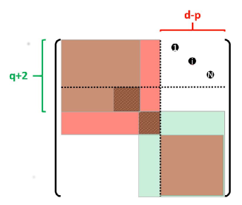
Figure 2: The figure illustrates our choice of coordinates on the conformal group. The blocks in red/green correspond to the left/right group $G_{p}/G_{q}$ while the additional generators $M_{i-1,p+1+i}$ are represented by block dots. The subgroup $B_{pq}$ of elements that commute with $M_{i-1,p+1+i},i=1,\dots,N$ is shown as the shaded area. Obviously, it is contained in the intersection of $G_{p}$ and $G_{q}$ (brown area).

Once we have fixed our coordinates on $G$ it is straightforward to compute first the metric and then the Laplace-Beltrami operator $\Delta_{\textrm{LB}}$ on $G$. The resulting expression is a second order differential operator that contains derivatives with respect to all the coordinates on the conformal group, including the coordinates $\tau_{i}$ on the torus $A_{pq}$ and the parameters $\lambda_{R}$ and $\lambda_{L}$ on the subgroups $D=\mathrm{SO}{(1,1)}$ of dilations in case $q=0$ or $p=q=0$. In order to descend to the space of conformal blocks we have to set all other derivatives to zero so that we end up with a second order differential operator $\Delta^{A}_{\textrm{LB}}$ in $\tau_{i}$. In case $q=0$ or $p=q=0$ the derivatives with respect to $\lambda_{R}$ and $\lambda_{L}$ are replaced by $-2a$ and $2b$, respectively. The operator $\Delta^{A}_{\textrm{LB}}$ still turns out to contain some first order terms. The latter can be removed by an appropriate “gauge transformation” (30). The Casimir operators $L^{2}$ we listed in the previous subsection are given by

$$L^{2}=\omega^{-1}\,\Delta^{A}_{\textrm{LB}}\,\omega\ .$$ (66)

It remains to relate the group theoretic variables $\tau_{i}$ we introduced through our parametrization of the conformal group $G$ to the cross-ratios. As we explained above, the location of the defect operators $\mathcal{D}^{(p)}(P_{\alpha})$ and $\mathcal{D}^{(q)}(Q_{\beta})$ can be characterized by a set of orthonormal vectors $P_{\alpha},\alpha=p+2,\dots,d+1,$ and $Q_{\beta},\beta=q+2,\dots,d+1,$ which are transverse to the defect in embedding space, respectively. We can complete these two sets to an orthonormal basis $\mathcal{P}$, $\mathcal{Q}$ of the full embedding space by adding vectors $\tilde{P}_{\alpha},\alpha=0,1,\dots,p+1,$ and $\tilde{Q}_{\beta},\beta=0,1,\dots,q+1$. Let us now combine these systems of orthonormal vectors into two matrices

$$\mathcal{P}=(\tilde{P},P)\in G=SO(1,d+1)\,,\quad\mathcal{Q}=(\tilde{Q},Q)\in G\,.$$ (67)

By construction, both $\mathcal{P}$ and $\mathcal{Q}$ carry a left action of the conformal group (since the columns are vectors in embedding space) and a right with respect to $G_{p}$ and $G_{q}$, respectively. The latter respects the split of the columns into vectors tangential and transverse to the defect. For the two $\mathrm{SO}{(1,d+1)}$ matrices $\mathcal{P}$ and $\mathcal{Q}$ we can now form the matrix $\mathcal{P}^{T}\mathcal{Q}\in\mathrm{SO}{(1,d+1)}$. Obviously, $\mathcal{P}^{T}\mathcal{Q}$ is invariant under conformal transformations, but it transforms non-trivially under the action of $G_{p}$ and $G_{q}$. In this way, any configuration of two defects of dimension $p$ and $q$ gives rise to an orbit $G_{p}\mathcal{P}^{T}\mathcal{Q}G_{q}$ in the double quotient $G_{p}\backslash G/G_{q}$.

In section 2 we considered the matrix $M=P^{T}Q$ in order to construct the cross-ratios $\eta_{i}$ of the defect configurations. Now we see that $M$ appears as the lower right matrix block of the matrix $a(\tau)$ we introduced in eq. (65). From the explicit construction in terms of the generators $M_{i-1,p+1+i}$ we can see that the lower right corner of $a(\tau)$ takes the form

$$\left(\begin{array}[]{@{}ccccc|c@{}}\cosh\frac{\tau_{1}}{2}&&&&&\\ &\cosh\frac{\tau_{2}}{2}&&&&\\ &&\ddots&&&0\\ &&&\cosh\frac{\tau_{N}}{2}&&\\ &&&&I&\end{array}\right)\,.$$ (68)

Comparison with our discussion of the cross-ratios allows us to read off the relation (32) between the group theoretic variables and cross-ratios.

The last task is to relate the Calogero-Sutherland eigenfunctions to the conformal blocks. In case of $p,q>0$, the Casimir equation for the correlator is the same as for the block (see eq. (16)). Hence we just need to undo the gauge transformation (30) and arrive at eq. (29). In case the defect configuration includes local fields, i.e.  when $q=0$ or $p,q=0$, the Casimir equations have been worked out Dolan:2003hv ; Billo:2016cpy and we arrive at eqs. (30) and (40), respectively. This concludes the brief sketch of the derivation of the results we listed in the first subsection. The interested reader can find many more details in Schomerus:2016epl where the case of scalar four-point blocks is analysed.

4 Calogero-Sutherland scattering states

Here we present a review of the solution theory. We introduce the fundamental domain of the Calogero-Sutherland problem and its fundamental (monodromy) group, Harish-Chandra scattering states, the monodromy representations and physical (monodromy free) wave functions.

4.1 Symmetries and fundamental domain

It is useful to consider the Calogero-Sutherland potential (3.1) as a function of $N$ complex variables first and to impose reality conditions a bit later. As a function of complex coordinates $\tau_{i}\in\mathbb{C}$, the potential possesses a few important symmetries. These include independent shifts of the coordinates $\tau_{i}$ by $2\pi i$ in the imaginary direction as well as two types of reflections, namely the inversion symmetries $\tau_{i}\leftrightarrow-\tau_{i}$ and the particle exchange symmetry $\tau_{i}\leftrightarrow\tau_{j}$. Together these form a non-abelian group that mathematicians refer to as affine Weyl group $\mathcal{W}_{N}$. The reflections actually generate a usual Weyl group and the shifts make this affine. The affine Weyl group is known to possess a so-called Coxeter representation through $N+1$ generators $w_{i},i=0,\dots,N$ with relations

$$\ w_{i}w_{j} = w_{j}w_{i}\quad\textrm{for}\ |i-j|\geq 2\,,$$ (69)

$$w_{i}w_{i+1}w_{i} = w_{i+1}w_{i}w_{i+1}\quad\textrm{for}\ i=1,\dots\,N-2\,,$$ (70)

$$w_{0}w_{1}w_{0}w_{1}=w_{1}w_{0}w_{1}w_{0} w_{N-1}w_{N}w_{N-1}w_{N}=w_{N}w_{N-1}w_{N}w_{N-1}\ .$$ , (71)

and

$$w_{i}^{2}=1\quad\textit{ for all}\quad i=0,\dots,N\ .$$ (72)

In this presentation of the affine Weyl group, the generators of the shifts in the imaginary direction are a bit hidden, but they can be reconstructed from the $w_{i}$, see van1983homotopy ; HeckmanBook .

The fundamental domain for the Calogero-Sutherland model is given by the quotient of the configuration space $\mathbb{C}^{N}$ with respect to the symmetries, i.e.

$$D_{N}=\mathbb{C}^{N}/\mathcal{W}_{N}\ .$$ (73)

We have depicted a 3-dimensional projection of the fundamental domain for $N=2$ in figure 3. Inside the wedge-shaped domain, the Calogero-Sutherland potential is finite but it diverges along the edges. We will refer to the hyperplanes of singularities as “walls” of the Calogero-Sutherland model. It turns out that the model possesses $N+1$ different walls $\omega_{i},i=0,\dots,N$, one for each generator $w_{i}$ of the affine Weyl group. For $N=2$ there are three such walls which are shown in figure 3. The possible real domains $A_{N}^{\alpha}$ of the model are given by the various faces of the domain $D_{N}$. Mathematicians usually study the Schroedinger problem in the real wedge $A_{N}^{+}$ which is given by $\tau_{i}\in\mathbb{R}$ with $\tau_{i}>\tau_{j}>0$ for all $i<j$.

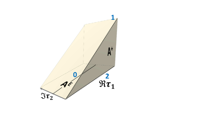
Figure 3: A 3-dimensional slice of the fundamental domain $D_{2}$ for the BC₂ Calogero-Sutherland model in $\tau$-space with $\Im\tau_{1}=0$. Front and back side of the wedge should be identified. The fixed points (walls) under the action of $w_{2}$ and $w_{1}$ are shown as bold dashed lines. Fixed points of $w_{2}$ fall into two disconnected components which carry the labels $0$ and $2$. The shaded area in front is the Weyl chamber $A_{2}^{+}$. It is bounded by the walls $\omega_{1}$ and $\omega_{2}$. The subset $A^{E}_{2}$ is the 2-dimensional semi-infinite strip of width $2\pi$ on the bottom of the wedge. It is bounded by the wall $\omega_{2}$, whereas wall $\omega_{0}$ cuts through its middle.

The fundamental group $\pi_{1}(D_{N})$ of the fundamental domain plays an important role in Calogero-Sutherland theory. It is generated by $N+1$ generators $g_{i}$ subject to the relations (69)-(71) with $w_{i}$ replaced by $g_{i}$. On the other hand, the generators $g_{i}$ of the fundamental group do not satisfy relation (72). The fundamental group of the domain $D_{N}$ is also referred to as affine braid group. Its relation to the affine Weyl group is like the relation between the braid group and the permutation group. Let us note that the generators $w_{a},a=1,\dots,N-1$ generate a subgroup $S_{N}\subset W_{N}$ of the affine Weyl group that is isomorphic to the symmetric group $S_{N}$. The corresponding generators $g_{a},a=1,\dots,N-1,$ within the monodromy group generate Artin’s braid group. In addition, the full monodromy contains two more generators, $g_{0}$ and $g_{N}$ which satisfy some fourth order ‘reflection type’ equations with $g_{1}$ and $g_{N-1}$, respectively.

4.2 Harish-Chandra scattering states

Before we enter our discussion of wave functions, it is advantageous to introduce a bit of notation. We shall denote by $e_{i},i=1,\dots,N,$ the $i^{\textrm{th}}$ unit vector in $\mathbb{C}^{N}$, i.e. the vector that is zero everywhere except in the $i^{\textrm{th}}$ entry which is one instead. From these unit vectors we build the following set $\Sigma^{+}$ of vectors in $\mathbb{C}^{N}$,

$$\Sigma^{+}=\{e_{i},2e_{i},e_{i}\pm e_{j}|1\leq i,j\leq N;i<j\}\ .$$ (74)

As one can easily count, the set contains $N(N+1)$ elements. Looking back at our Calogero-Sutherland potentials we observe that they contain one summand for each element in $\Sigma^{+}$. In fact, we can also write the potential as

$$V^{\text{CS}}(\tau_{i})=\sum_{\alpha\in\Sigma^{+}}\frac{k_{\alpha}(k_{\alpha}+2k_{2\alpha}-1)\langle\alpha,\alpha\rangle}{4\sinh^{2}\frac{\langle\alpha,\tau\rangle}{2}}\ .$$ (75)

where the scalar product $\langle\cdot,\cdot\rangle$ is normalized such that $\langle e_{i},e_{j}\rangle=\delta_{i,j}$ and we assembled all the coordinates $\tau_{i}\in\mathbb{C}$ into a vector $\tau=\sum_{i}\tau_{i}e_{i}$ with

$$k_{e_{i}}=k_{1}\quad,\quad k_{2e_{i}}=k_{2}\quad,\quad k_{e_{i}\pm e_{j}}=k_{3}\ .$$

Let us agree to extend the definition of $k_{\alpha}$ to arbitrary elements $\alpha\in\mathbb{R}^{N}$ such that is vanishes whenever $\alpha\not\in\Sigma^{+}$. Just as in the case of the potential, many formulas below will turn out to become much simpler when written as sums or products over the set $\Sigma^{+}$.

With these notations set up let us come to our main subject, namely the study of wave functions. Since the Calogero-Sutherland potential falls off at $\tau_{i}\rightarrow\infty$, any wave function becomes a superposition of plane waves in this asymptotic regime. In mathematics is it customary to factor off the ground state wave function of the trigonometric Calogero-Sutherland model, i.e. of the Hamiltonian that is obtained when all the $\tau_{i}$ are purely imaginary. This ground state wave function $\Theta$ is explicitly known,

$$\Theta(\tau_{i})=\ \prod_{\alpha\in\Sigma^{+}}\left(2\sinh\frac{\langle\alpha,\tau\rangle}{2}\right)^{k_{\alpha}}\ .$$ (76)

For the wave function of the the Calogero-Sutherland model on the domain $A_{N}^{+}$ we make the Ansatz

$$\Psi(\lambda,k;\tau)=\Theta(k;\tau)\Phi(\lambda,k;\tau)\ .$$ (77)

Let us note in passing that the function $\Theta(k,\tau)$ possesses the following asymptotics for large $\tau$,

$$\Theta(k;\tau) \sim e^{\langle\rho_{k},\tau\rangle}+\dots\quad\textit{where}\quad$$ (78)

$$\rho_{k} := \left(\frac{k_{1}}{2}+k_{2}+(N-1)k_{3},\frac{k_{1}}{2}+k_{2}+(N-2)k_{3},\dots,\frac{k_{1}}{2}+k_{2}\right)\ .$$

So-called Harish-Chandra wave functions $\Phi(\lambda,k;\tau)$ are $W_{N}$ symmetric solutions of the Calogero-Sutherland Hamiltonian for which $\Phi$ possesses the following simple asymptotic behavior

$$\Phi(\lambda,k;\tau)\ \sim\ e^{\langle\lambda-\rho_{k},\tau\rangle}+\dots\ \mbox{ for }\ \tau\rightarrow\infty\ \mathrm{in}\ A^{+}_{N}=\textit{WC}_{N}$$ (79)

where $\lambda=\sum_{i}\lambda_{i}e_{i}$ and $\tau\rightarrow\infty$ in $A^{+}_{N}$ means that all components become large while preserving the order $\tau_{N}<\tau_{N-1}<\dots<\tau_{1}$. Imposing $W_{N}$ symmetry implies that as a function of $\tau_{i}$, $\Phi$ is reflection symmetric and invariant under any permutation of the $\tau_{i}$. The condition (79) selects a unique solution of the scattering problem describing a single plane wave. It is analytic in the wedge $A^{+}_{N}$. The corresponding eigenvalue of the Calogero-Sutherland Hamiltonian is given by

$$\varepsilon=\varepsilon(\lambda)=-\sum\lambda_{i}^{2}\ .$$

When we required the Harish-Chandra functions to be symmetric, we used the action of the Weyl group $W_{N}$ on the coordinate space. On the other hand, the Weyl group also acts in a natural way on the asymptotic data $\lambda$ of the Harish-Chandra functions by sending any choice of $\lambda$ through a sequence of Weyl reflections to $w\lambda,w\in W_{N}$. In particular, the generators $w_{j},j=1,\dots,N$ act as

$$w_{a}\lambda_{i}=\delta_{a+1,i}\lambda_{i-1}+\left(1-\delta_{a,i}\right)\left(1-\delta_{a+1,i}\right)\lambda_{i}+\delta_{a,i}\lambda_{i+1}\quad,\quad w_{N}\lambda_{i}=(-1)^{\delta_{N,i}}\lambda_{i}\$$ (80)

for $a=1,\dots,N-1$ and $i=1,\dots,N$. Since the eigenvalue $\varepsilon$ is invariant under exchange and reflection of the momenta $\lambda_{i}$, our Harish-Chandra functions come in families. For generic choices of $\lambda$, one obtains $|W_{N}|=N!2^{N}$ solutions $\Phi(w\lambda,k;\tau)$ which all possess the same eigenvalue of the Hamiltonian.

At least for sufficiently generic values of the momenta, Harish-Chandra functions possess a series expansion in the variables $x_{i}=\exp\tau_{i}$

$$\Phi(\lambda,k;\tau)=\sum_{\mu\in Q_{+}}\Gamma_{\mu}(\lambda,k)e^{\langle\lambda-\rho_{k}-\mu,\tau\rangle},\quad\quad\Gamma_{0}(\lambda,k)=1,$$ (81)

where we adopt $|\Im\tau_{i}|<\pi$ for $i=1,\dots,N$ on the principal branch of BC_N Harish-Chandra functions and we sum over elements $\mu$ of the integer cone

$$Q_{+}=\{\mu=\sum_{a=1}^{N-1}n_{a}(e_{a}-e_{a+1})+ne_{N}\,|\,n_{a},n\geq 0\ \textrm{for}\ a=1,\dots,N-1\,\}\ .$$

By inserting this formal expansion into the Calogero-Sutherland eigenvalue equations one can easily derive equations for the expansion coefficients $\Gamma_{\mu}$ that may be solved recursively, at least for generic eigenvalues $\lambda_{i}$. In a few cases, explicit formulas for $\Gamma_{\mu}$ are also known. For $N=2$, for example, the series expansion of Harish-Chandra functions with generic eigenvalues $\lambda_{i}$ was recently worked out in Isachenkov:2017qgn , generalizing earlier expressions by Dolan and Osborn that were only valid for cases in which $\lambda_{1}-\lambda_{2}-k_{3}$ is non-negative integer. The procedure that was employed in Isachenkov:2017qgn can in principle be extended to $N>2$. This remains an interesting challenge for future work.

In Heckman-Opdam theory many properties of the Harish-Chandra functions have been obtained without knowing the explicit series expansions. In particular let us mention that the functions $\exp(\langle-\lambda+\rho(k),\tau\rangle)\Phi(\lambda;k;\tau)$ are known to be entire functions of the multiplicities $k_{i}$ and meromorphic functions of asymptotic data $\lambda_{i}$, for any fixed choice of $\tau$ in the fundamental domain. They are known to possess simple poles whenever the set of $\lambda_{i}$ satisfies one of the following conditions

$$\langle\lambda_{\ast},\alpha\rangle=\frac{s}{2}\langle\alpha,\alpha\rangle\quad\textrm{for}\quad s=1,2,\dots\quad,\quad\alpha\in\Sigma^{+}\ .$$ (82)

For the poles at $\lambda_{\ast}=\lambda_{\alpha,n}$, the residues are given by (see e.g. OpdamDunkl )

$$\text{Res}_{(\alpha,s)}\Phi(\lambda,k;\tau)\sim\Phi(w(\alpha)\lambda_{\alpha,s},k;\tau)\ .$$ (83)

where $\sim$ indicates that the relation with the Harish-Chandra function on the right hand side holds only up to a constant factor. The latter is not known in general, but it can be found from the series expansion as in Isachenkov:2017qgn for $N=2$. The Harish-Chandra function on the right hand side is related to the one on the left by acting with an element $w(\alpha)\in W_{N}$ of the Weyl group on the set of momenta $\lambda_{i}$, defined in (80). A complete discussion of poles and residues for $N=2$, including non-generic momenta $\lambda_{i}$ can be found in Isachenkov:2017qgn .

4.3 Monodromy representation and wave functions

The scattering states we have discussed in the previous subsection fail to be good wave functions for the various real slices one may consider. In fact, at infinity Harish-Chandra function contains a single plain wave. On the other hand, the latter are not regular at the walls of the scattering problem. Finding true wave functions requires to impose regularity conditions at the walls and hence forces us to consider certain linear combinations of the $2^{N}N!$ Harish-Chandra functions with given energy $\varepsilon$.

The behavior of all wave functions at the walls is encoded in the monodromy representation of the fundamental group. As we saw above, the fundamental group, which in our case has been identified as the affine braid group, contains one generator $g_{i},i=0,\dots,N$ for each of the walls. The representation of this generator encodes how wave functions behave as we continue along a curve that surrounds the wall. Note that all walls possess real co-dimension two since they are defined by one complex linear equation. The $2^{N}N!$-dimensional space of Harish-Chandra functions $\Phi(w\lambda,\tau),w\in W_{N}$ carries a representation of the monodromy group. The representation matrices $M_{i}=M(g_{i})$ are explicitly known from the work of Heckman and Opdam, see Isachenkov:2017qgn for explicit formulas. In the special case of $N=2$, expressions for two of the three monodromy matrices were also worked out in the conformal field theory literature Caron-Huot:2017vep . Let us stress that these matrices satisfy the relations (69)-(71) that are the defining relation of the affine braid group. In addition they turn out to obey the following set of Hecke relations

$$(M_{r}-1)(M_{r}-\gamma_{r}) = 0\quad,\quad\mathrm{where}\$$ (84)

$$\gamma_{0}=e^{\pi i(2k_{2}-1)}\ ,\ \gamma_{i} = e^{\pi i(2k_{3}-1)}\ ,\ \gamma_{N}=e^{\pi i(2k_{1}+2k_{2}-1)}\$$

for $r=0,\dots,N$ and $i=1,\dots,N-1$. These may be considered as a deformation of the relations (72). In this sense, this monodromy representation of the affine braid group is rather close to being a representation of the affine Weyl group. For generic values of the multiplicities $k$ and momenta $\lambda$, the monodromy representation of the affine braid group on Harish-Chandra functions is irreducible. The precise condition is

$$2\frac{\langle\lambda,\alpha\rangle}{\langle\alpha,\alpha\rangle}\not\in\mathbb{Z}\quad and\quad 2\frac{\langle\lambda,\alpha\rangle}{\langle\alpha,\alpha\rangle}+\frac{k_{\alpha/2}}{2}+k_{\alpha}\not\in\mathbb{Z}$$ (85)

for all elements $\alpha\in\Sigma^{+}$. When one of these conditions is violated, the monodromy representation may contain non-trivial subrepresentations.

In terms of these monodromy matrices, regularity of the wave function $\Phi$ at a wall $\omega_{i}$ is equivalent to $\Phi$ being an eigenfunction of the corresponding monodromy matrix $M_{i}=M(g_{i})$ with unit eigenvalue, i.e. $\Phi$ is regular along $\omega_{i}$ if and only if $M_{i}\Phi=\Phi$. There exists a very simple prescription how to build a function $\Phi$ that is analytic at some subset $\omega_{i_{1}},\dots,\omega_{i_{r}}$ consisting of $r\leq N$ of the $N$ walls that bound $A^{+}_{N}$, i.e  $i_{\nu}\neq 0$. For each of these walls there is a generator $w_{i_{\nu}}$ of the Weyl group and so our set of $r$ walls is associated with a subgroup $V\subset W_{N}$ of the Weyl group that is generated by $w_{i_{1}},\dots,w_{i_{r}}$. Given this subgroup we now define the following superposition of Harish-Chandra functions

$$\Phi^{V}(\lambda,k;\tau)=\sum_{w\in V}c(w\lambda,k)\Phi(w\lambda,k;\tau)$$ (86)

where the so-called Harish-Chandra c-function reads

$$c(\lambda,k) = \frac{\gamma(\lambda,k)}{\gamma(\rho(k),k)}\quad,\quad\gamma(\lambda,k)=\prod_{\alpha\in\Sigma^{+}}\gamma_{\alpha}(\lambda,k)\quad,$$ (88)

$$\gamma_{\alpha}(\lambda,k)=\frac{\Gamma\left(\frac{1}{2}k_{\alpha/2}+\langle\lambda,\alpha^{\vee}\rangle\right)}{\Gamma\left(\frac{1}{2}k_{\alpha/2}+k_{\alpha}+\langle\lambda,\alpha^{\vee}\rangle\right)}.$$

For future convenience, let us also introduce

$$\gamma_{\alpha}^{*}(\lambda,k)=\frac{\Gamma\left(1-\frac{1}{2}k_{\alpha/2}-k_{\alpha}-\langle\lambda,\alpha^{\vee}\rangle\right)}{\Gamma\left(1-\frac{1}{2}k_{\alpha/2}-\langle\lambda,\alpha^{\vee}\rangle\right)}.$$ (89)

Any wave function of the form (86) turns out be be regular at the walls $\omega_{i_{1}},\dots,\omega_{i_{r}}$. Physical wave functions on the Weyl chamber $A^{+}_{N}$ are obtained when $V=W_{N}$ is the entire Weyl group, the most well studied case in the mathematical literature. For this choice of $V$ we end up with one unique linear combination of Harish-Chandra functions for each Weyl-orbit of $\lambda$. The functions $F^{+}_{N}=\Phi^{W_{N}}$ are known as Heckman-Opdam hypergeometric function. They are close cousins of the Lorentzian hypergeometric functions that were introduced in Isachenkov:2017qgn . The set of true wave functions $F^{+}_{N}(\lambda,\tau)$ of the Calogero-Sutherland model gives rise to an orthonormal basis of functions on the wedge $A^{+}_{N}$. Let us note, however, that, while the functions $F^{+}_{N}$ are analytic in a neighborhood of $A^{+}_{N}$, they fail to be analytic at the wall $\omega_{0}$. Other real domains whose boundary contains the wall $\omega_{0}$, are associated with different subgroups of the affine Weyl group. Which subgroup one has to sum over in order to obtain an orthonormal basis of wave functions and the precise form of coefficients in this sum depend on the chosen domain for the Calogero-Sutherland scattering problem.

5 Euclidean inversion formula and defect blocks

After our sketch of the solution theory for Calogero-Sutherland models we are now in a position to construct conformal partial waves and blocks. In the next subsection we shall explain how to build the conformal partial waves explicitly in terms of Harish-Chandra functions. By definition, conformal partial waves are the physical wave functions on the Euclidean domain, i.e. single valued solutions of the Casimir equation in Euclidean kinematics. Our analysis provides one with a complete basis of such wave functions and hence with a Euclidean inversion formula. In the final subsection we shall also construct and discuss the conformal blocks that were introduced in section 2.3, thereby completing the main goal of this work.

5.1 Euclidean hypergeometrics and inversion formulas

The Heckman-Opdam hypergeometric functions we described briefly in the final paragraph of the previous section, provide physical wave functions for the domain $A^{+}_{N}$. Their construction is well known in the mathematical literature. To obtain the Euclidean inversion formula for defects, we are mostly interested in the physical wave functions for the Euclidean domain $A^{E}_{N}$ that was introduced in eq. (32). As far as we know, there exists no general theory for these functions, but for the specific example of $N=2$ that is associated to scalar four-point blocks, such wave functions have been known in the context of conformal field theory for a long time, see e.g. Costa:2012cb ; Caron-Huot:2017vep for explicit formulas in the recent literature. Here we shall generalize these functions to $N\geq 2$ using the characterization that was proposed in Isachenkov:2017qgn .

Before we can characterize the physical wave functions we need to introduce a bit of notation. In eq. (32) we have introduced the domain $A^{E}_{N}$. Of course, there are quite a few walls within $A_{N}^{E}$. When we consider the Calogero-Sutherland problem it is natural to first formulate it in a smaller domain that is bounded by walls but does not have walls in the interior. Here we shall describe such a small domain $D^{E}_{N}$ and then explain how to glue $A_{N}^{E}$ from the small domain $D^{E}_{N}$ and some of its images under the action of the affine Weyl group. In order to do so we first define the simplex $\triangle_{N-1}$ that is parametrized by an ordered set of $N-1$ angles $\theta_{i}$

$$\triangle_{N-1}:=\{(\theta_{i},\dots,\theta_{N-1})\,|\,\theta_{i}\in[0,\pi/2[;\theta_{i}\geq\theta_{j}\ \mbox{for}\ i<j\}\ .$$ (90)

We can then introduce the domain $D^{E}_{N}$ as a semi-infinite cylinder over $\triangle_{N-1}$, i.e.

$$D_{N}^{E}\>=\{(\vartheta,\theta_{i})\,|\,\vartheta\in\mathbb{R}^{+}_{0}\,;\,(\theta_{i})\in\triangle_{N-1}\,\}\ .$$ (91)

The hypercubic base of our the Euclidean domain $A^{E}_{N}$ that was introduced in eq. (32) can be triangulated into a disjoint union of the simplex $\triangle_{N-1}$ an its reflections under the following subgroup $W^{B}_{N}$ of the Weyl group $W_{N}$,

$$W^{B}_{N}\colonequals\{w_{2},\dots,w_{N-1},w_{N}\,\,|\,\text{ relations of }W_{N}\}\ \subset W_{N}\,.$$ (92)

More precisely, our Euclidean domain $A^{E}_{N}$ can be decomposed as

$$A_{N}^{E}\ =\ \bigsqcup_{w\in\varkappa\cdot W^{B}_{N}}\,wD_{N}^{E},$$ (93)

where $\varkappa$ is an element of affine Weyl group which simultaneously shifts all the angular variables. Explicitly, $\varkappa$ acts on the coordinates as $\varkappa:\theta_{j}\mapsto\theta_{j}+\pi/2$ for $j=1,\dots,N-1$ or, equivalently, in terms of the variables $\tau_{j}$, it is given by $\varkappa:\tau_{j+1}\mapsto\tau_{j+1}+i\pi$, $j=1,\dots,N-1$, while leaving $\tau_{1}$ invariant. Let us stress that in the decomposition formula (93) the Weyl group elements $w$ act on coordinates, not on momenta as in most other formulas.

The boundary of $D^{E}_{N}\subset\mathbb{R}^{N}$ runs along various walls of our Calogero-Sutherland problem. In fact, the simplex $\triangle_{N-1}$ which appears at $\tau_{1}=0$, runs along the wall $\omega_{N}$ acted upon with the Weyl reflection $w_{1}w_{2}\cdots w_{N-1}$. There are also two semi-infinite cells of the boundary defined by $\tau_{N}=0$ and $\tau_{2}=i\pi$ which are part of the wall $\omega_{N}$, and of its image under the Weyl reflection $w_{2}\cdots w_{N-1}$, respectively. Finally, the boundary components at $\tau_{A}=\tau_{A+1},A=2,\dots,N-1$ run along the walls $\omega_{A}$ for $A=2,\dots,N-1$.

We are looking for a physical wave function that is regular along the entire boundary of the domain $D^{E}_{N}$. From our description of the boundary in the previous paragraph it is clear that such a wave function can be characterized through the following set of monodromy conditions:

$$M_{1}^{-1}\cdots M_{N-1}^{-1}M_{N}M_{N-1}\cdots M_{1}F^{E}(\lambda_{i};k_{a};\tau_{i}) = F^{E}(\lambda_{i};k_{a};\tau_{i})\,,$$

$$M_{N}F^{E}(\lambda_{i};k_{a};\tau_{i}) = F^{E}(\lambda_{i};k_{a};\tau_{i})\,,$$ (94)

$$M_{A}F^{E}(\lambda_{i};k_{a};\tau_{i}) = F^{E}(\lambda_{i};k_{a};\tau_{i}),\,$$

where $A=2,\dots,N-1$. The conditions we have displayed here do not directly impose triviality of the monodromy along $\tau_{2}=i\pi$. Note however that the monodromy along the wall $\tau_{2}=0$ is given by the matrix $M_{2}^{-1}\cdots M_{N-1}^{-1}M_{N}\cdots M_{2}$. Since the monodromy matrix along this wall is simply a product of monodromy matrices we trivialized, the functions $F^{E}$ are automatically regular along $\tau_{2}=0$. According to our discussion above, this ensures that the monodromy along the wall $\tau_{2}=i\pi$ is trivial as well, as long as we impose appropriate discretization conditions on the momenta $\lambda$. If the discretization conditions are violated, on the other hand, the functions $F^{E}$ will possess branch cuts along the wall at $\tau_{2}=i\pi$.

In building the relevant solutions to the set of conditions (94), let us first look at the case of $N=2$ for which we only need to trivialize the monodromies $M_{2}$, $M_{1}^{-1}M_{2}M_{1}$, along with $\tilde{M}_{2}$ which corresponds to the wall $\tau_{2}=\pi i$. The corresponding reflections form a Klein-four subgroup

$$\mathbb{Z}_{2}^{2}=\{1,w_{2},w_{1}w_{2}w_{1},w_{1}w_{2}w_{1}w_{2}\}\subset W_{2}$$

of our Weyl group $W_{2}$ for $N=2$. Using the expressions for monodromy matrices from HeckmanBook , the solution to eqs. (94) is seen to take the form

$$F^{E}_{N=2}(\lambda_{i};k_{a};\tau_{i})=\sum_{w\in\mathbb{Z}_{2}^{2}}\gamma^{E}_{N=2}(w\lambda,k)\Phi(w\lambda_{i};k_{a};\tau_{i})\,,$$ (95)

where

$$\gamma^{E}_{N=2}\left(\lambda,k\right)\colonequals\gamma^{*}_{e_{1}-e_{2}}\left(\lambda,k\right)\prod_{\alpha\in\Sigma^{+}\backslash\{e_{1}-e_{2}\}}\gamma_{\alpha}\left(\lambda,k\right)\ .$$

We claim that the functions $F^{E}$ form a basis of the space of functions on the Euclidean domain provided that we let $\lambda_{i}$ run through

$$\lambda_{1}=\frac{d}{4}-\frac{\Delta}{2}=i\frac{\text{p}}{2}\quad\textit{ and }\quad\lambda_{2}=\frac{d-2}{4}+\frac{\ell}{2}\quad\textit{ for }\quad\ell=0,2,4,\dots$$

where p is a non-negative real number. The simplest way to see that the basis of such Euclidean hypergeometric functions will be labeled by even spins $\ell$ is to notice that the monodromy conditions imposed on all non-compact walls of $D_{N}^{E}$ are essentially those for regularity of a $\textit{BC}_{1}$ Jacobi polynomial of $\cos\tau_{2}/i=\cos 2\theta_{1}$ with $\rho_{0}=d/4-1/2$. The latter is known to form orthogonal system on the ’simplex’ $\triangle_{1}$, i.e. $\tau_{2}/i\in[0,\pi[$, only for the discrete set of momenta we have displayed. By symmetry $\tilde{\varrho}$ of the $\textit{BC}_{1}$ polynomial problem, these uniquely extend to the eigenfunctions on our base ’hypercube’ $\{\theta_{1}\in[0,\pi[\}$, preserving the scalar product. Correspondingly, the Euclidean hypergeometric function above is defined on the whole Euclidean strip $A_{1}^{E}$, starting from the smaller strip $D_{1}^{E}$.

With this experience from $N=2$ we now turn to general $N$. The walls of $D_{N}^{E}$ whose monodromy we need to trivialize are in one-to-one correspondence with reflections in the Weyl group. The latter generate a subgroup $W^{E}_{N}$ of the Weyl group $W_{N}$,

$$W^{E}_{N}\colonequals\{w_{2},\dots,w_{N-1},w_{N},w_{E}\,\,|\,\text{ relations of }W_{N}\}\ \subset W_{N}\,$$ (96)

where we introduced a shorthand

$$w_{E}\colonequals w_{1}w_{2}\dots w_{N}w_{N-1}\dots w_{1}.$$ (97)

Let us remind that $D_{N}^{E}$ possesses one wall, namely the wall along $\tau_{1}=i\pi$ that is not associated with a reflection. But as we discussed above, its monodromy is trivialized automatically once we have taken care of all the other walls and imposed the discretization conditions. The subgroup $W^{E}_{N}$ has index $N$ in $W_{N}$. To spell out the Euclidean hypergeometric functions in this case, we denote

$$\Sigma_{\star}^{+}\colonequals\{e_{1}-e_{j}\,|\,j=2,\dots,N\},$$ (98)

and

$$\gamma^{E}\left(\lambda,k\right)\colonequals\prod_{\alpha\in\Sigma_{\star}^{+}}\gamma^{*}_{\alpha}\left(\lambda,k\right)\prod_{\alpha\in\Sigma^{+}\backslash\Sigma_{\star}^{+}}\gamma_{\alpha}\left(\lambda,k\right).$$ (99)

Then the corresponding solution of the monodromy conditions eqs. (94) takes the form

$$F^{E}(\lambda_{i};k_{a};\tau_{i})=\sum_{w\in W^{E}_{N}}\gamma^{E}(w\lambda,k)\Phi(w\lambda_{i};k_{a};\tau_{i})\,.$$ (100)

For later use let us note that these functions $F^{E}$ are invariant under the action of the Weyl reflection $w_{E}$, i.e.

$$F^{E}(w_{E}\lambda_{i};k_{a};\tau_{i})=F^{E}(\lambda_{i};k_{a};\tau_{i})\$$

simply because the sum over $W^{E}_{N}$ includes a sum over $\{1,w_{E}\}$. The Euclidean wave function (or partial wave) (100) is naively a sum over $2^{N}(N-1)!$ Harish-Chandra (or pure) functions. In fact, though, most of the coefficients vanish once we impose the appropriate integrality conditions on the eigenvalues $\lambda_{i}$ (as it happens in the case of scalar four-point functions), leaving just two non-zero Harish-Chandra functions with labels $\lambda=(\lambda_{1},\lambda_{2},\dots,\lambda_{N})$ and $w_{E}\lambda=(-\lambda_{1},\lambda_{2},\dots,\lambda_{N})$. Namely, we obtain a complete basis of wave functions if we let $\lambda_{i},i=1,\dots,N$ run through the set

$$\lambda_{1}=\frac{d}{4}-\frac{\Delta}{2}=i\frac{\text{p}}{2}\quad\textit{and }\quad\lambda_{j+1}=\frac{d}{4}+\frac{l_{j}-j}{2}\quad\textit{ with }\quad j=1,\dots,N-1,\quad l_{j}=0,2,4,\dots$$ (101)

where p is a non-negative real number, as before. Note that the monodromy conditions imposed on all non-compact walls of $D_{N}^{E}$ are essentially those for regularity of a $\textit{BC}_{N-1}$ Jacobi polynomial of $\left(\cos 2\theta_{1},\dots\cos 2\theta_{N-1}\right)$ with

$$\rho_{B}=\rho_{k}^{(N-1)}=(d/4-1/2,d/4-2/2,\dots,d/4-(N-1)/2)\ .$$

Here, $\rho_{k}$ is the vector we introduced in eq. (78), but for the $\textit{BC}_{N-1}$ root system. These Jacobi polynomials are known to form an orthogonal system on a simplex $\triangle_{N-1}$ only if $(\lambda_{2},\dots,\lambda_{N})\in\rho_{B}+P^{+}_{B}$, where

$$P^{+}_{B}=\{(\nu_{1},\dots,\nu_{N-1})\in\mathbb{Z}_{\geq 0}^{N-1}\,\,|\,\,\nu_{1}\geq\cdots\geq\nu_{N-1}\}$$

is a set of dominant weights of $\textit{BC}_{N-1}$ root system. As in the $N=2$ case, by symmetries of the $\textit{BC}_{N-1}$ polynomial problem, these possess a unique continuation to the eigenfunctions on our base hypercube $\{\theta_{j}\in[0,\pi[\}$, $j=1,\dots,N-1$, such that the scalar product is preserved. Correspondingly, the Euclidean hypergeometric function above is defined on the whole Euclidean domain $A_{N}^{E}$, starting from the smaller domain $D_{N}^{E}$. Our basis functions on $A^{E}_{N}$ are labeled by Young diagrams with even row lengths $2\nu_{1}\geq\cdots\geq 2\nu_{N-1}\geq 0$, $\nu_{i}\in\mathbb{Z}$, corresponding to spins $l_{i}=2\nu_{i}$, $i=1,\dots,N-1$ of a defect partial wave.

A more formal proof of the orthogonality statement goes via Heckman-Opdam shift operators Heckman1991 ; HeckmanBook as follows. First one writes down the inversion for $k_{3}=0$, when orthogonality trivially splits into applications of polynomial $\textit{BC}_{N-1}$ and non-polynomial Jacobi (i.e. $\textit{BC}_{1}$) inversion formulas. One then inserts a resolution of the identity $1=G_{-}^{k_{3}}*G_{+}^{k_{3}}$ via multiplicity shift operators $G_{\pm}$ for the $k_{3}$ orbit (appropriately normalized on Euclidean wave functions by Harish-Chandra isomorphism alg-structures ) into the scalar product of the $k_{3}=0$ Euclidean hypergeometric functions which, by transposition, gives the result for a countable set of values $k_{3}=0,1,2,\dots$. To finalize, one should apply an analytical argument in the spirit of Carlson’s lemma AAR and continue to a dense subset of multiplicities, see HeckmanBook for samples of such calculations for Calogero-Sutherland wave functions.

As we have just established, the functions we have constructed in eqs. (100) and (101) form a complete and orthogonal set of wave functions for the Calogero-Sutherland scattering problem in the Euclidean domain. In particular, we can use them to project correlation functions $G$ for two defects onto conformal blocks, see also HeckmanBook ,

$$\mathcal{\tilde{C}}(\lambda_{i})=\frac{(N-1)!}{(i\pi)^{N-1}}\int_{D^{E}_{N}}\prod_{j=1}^{N}d\tau_{j}\,\left|\Theta(\tau_{i};k_{a})\right|^{2}\,F^{E}(\lambda_{i};k_{a};\tau_{i})\,G(\tau_{i})\,.$$ (102)

According to the discussion above, we can extend this integral transform to the whole Euclidean region $A_{N}^{E}$, which then reads as

$$\mathcal{C}(\lambda_{i})=\int_{A^{E}_{N}}d\tau_{1}\,\frac{\prod_{j=2}^{N}d\tau_{j}}{\left(2\pi i\right)^{N-1}}\,\left|\Theta(\tau_{i};k_{a})\right|^{2}\,F^{E}(\lambda_{i};k_{a};\tau_{i})\,G(\tau_{i})\,.$$ (103)

The measure factor $\Theta$ was introduced in eq. (76) above and the integration is over the domain $A^{E}_{N}$. Convergence of the above integral is assured if $-1<p<d-1$ for the setup of two point functions in presence of a defect ($N=2$) and $-1<p-q<3-2N+d$ for the setup of defect two point functions ($N\geq 2$). In those cases with $N=2$ cross ratios that have previously appeared in the conformal field theory literature, our normalization differs a bit from the usual one. We will give precise relations below. For later applications we note that our conventions guarantee that $\mathcal{C}$ possesses the following shadow symmetry,

$$\mathcal{C}\left(\lambda\right)=\mathcal{C}\left(w_{E}\lambda\right)\,.$$ (104)

Using the orthogonality properties of the partial waves $F^{E}$ we can invert formula (103) to decompose the correlation function into a sum/integral over wave functions,

$$G(\tau_{i})=\sum_{\begin{subarray}{c}l_{1}\geq\dots\geq l_{N-1}\geq 0\\ l_{i}\text{ even}\end{subarray}}^{\infty}\int_{0}^{\infty}\frac{d\text{p}}{4\pi}\,\mu(\lambda;k_{a})\,F^{E}(\lambda_{i};k_{a};\tau_{i})\,\mathcal{C}(\lambda_{i})\,,$$ (105)

where $\lambda_{i}$ are considered as functions of $l_{i}$ and $p$, see eq. (101), and the measure $\mu$ is given by

$$\mu(\lambda;k_{a})=\prod_{\alpha\in\Sigma_{B}^{+}}\left(\frac{\gamma_{\alpha}\left(\lambda,k\right)}{\gamma_{\alpha}^{*}\left(-\lambda,k\right)}\right)\frac{1}{\gamma^{E}\left(\lambda,k\right)\gamma^{E}\left(w_{E}\lambda,k\right)}\,.$$ (106)

Here, the product runs over the following a subsystem $\Sigma^{+}_{B}$ of the root system $\Sigma^{+}$,

$$\Sigma^{+}_{B}=\{e_{i},2e_{i},e_{i}\pm e_{j}|2\leq i,j\leq N;i<j\}\ .$$ (107)

Reflections in $\mathbb{C}^{N-1}$ with respect to the roots of this rank $N-1$ system generate the Weyl group $W_{N-1}$ of $\textit{BC}_{N-1}$. The integral over p runs along the positive real numbers, or equivalently the $\Delta$ integration runs along the half-line $\Delta=d/2-i\text{p}$ of principal series representations. As usual, if some poles of gamma functions in the measure start to cross this line, bound states start to appear in the spectrum corresponding to residues of the measure at these poles, which would be equivalent to a Mellin-Barnes prescription for the corresponding integral in $\lambda_{1}$ over the full imaginary line. In particular, one can notice that residues appear for $p>d/2$ in the case of a two point function in presence of a defect ($N=2$) and for $p-q>2+d/2-N$ in the case of a two point function of defects ($N\geq 2$). If the function $\mathcal{C}(\lambda)|_{\lambda_{1}=i\text{p}/2}$ has residues in p to the bottom of the integration line, a contour should be moreover indented to encircle this residue in such a way that no shadow contribution is picked, in full analogy with the case of four-point function. Using the shadow symmetry (104) of the function $\mathcal{C}$, the integration over a half-line becomes integration over the entire imaginary line, so that by closing contour in the lower half-plane and taking residues with the above prescriptions, one reproduces a bulk operator product expansion. We conclude the list of subtleties with mentioning that, if poles of blocks themselves appear in the lower half-plane, they should be taken care of in order not to mix with physical poles, see our description of poles of Calogero-Sutherland wave functions in section 4.

Since our formulas for the measure factors $|\Theta|^{2}$ and $\mu$ in eqs.  (103) and (105) may look a little abstract at first, let us spell out more explicit expressions for $N=2$. In this case, eqs. (76) and (106) give

$$\frac{\left|\Theta(\tau_{i};k_{a})\right|^{2}_{N=2}}{4^{d-1+2a}}=\left(\sinh^{2}\vartheta\,\sin^{2}\theta_{1}\right)^{\frac{d-p}{2}-1}\left(\cosh^{2}\vartheta\,\cos^{2}\theta_{1}\right)^{\frac{p}{2}}\left(\sinh^{2}\vartheta+\sin^{2}\theta_{1}\right)^{2a+1}$$

and

$$\mu(\lambda;k_{a})_{N=2}= \frac{4^{d-2p-4}}{2\pi}\left(\ell+\frac{d}{2}-1\right)\left(\Delta+\ell-1\right)\left(d-\Delta+\ell-1\right)\frac{\Gamma\left(\frac{d-p+\ell-1}{2},\frac{d+\ell}{2}-1\right)}{\Gamma\left(\frac{\ell+p+1}{2},\frac{\ell}{2}+1\right)}$$

$$\times\frac{\Gamma\left(\frac{\Delta-1}{2},\frac{\Delta-p}{2},\frac{d-\Delta-1}{2},\frac{d-\Delta-p}{2},\frac{\Delta+\ell}{2}+a,\frac{d-\Delta+\ell}{2}+a\right)}{\Gamma\left(\pm\left(\Delta-\frac{d}{2}\right),\frac{\Delta+\ell}{2}-a,\frac{d-\Delta+\ell}{2}-a\right)}.$$

Here we used the standard notation that a $\Gamma$ function with multiple arguments is given by a product, i.e.  $\Gamma(a,X)=\Gamma(a)\Gamma(X)$, and $\Gamma(a\pm b)=\Gamma(a+b)\Gamma(a-b)$. For higher values of $N$, the inversion formula may be a bit more cumbersome to write out explicitly, but all necessary formulas were spelled out above. Equation (103) is the Euclidean inversion formula we were after in this section. It is a vast generalization of the Euclidean inversion formula for scalar four-point functions.

As we have noted above, our normalization conventions for the correlation functions $G$ as well as for the measure factors differ a bit from those used in the existing conformal field theory literature on two point functions in the presence of a defect. For a direct comparison one should apply the following list of re-definitions,

$$\mathcal{F}^{\text{CFT}}\left(\tau_{i}\right)=4^{\frac{d}{2}+2a}\,\left(\sinh\frac{\tau_{1}\pm\tau_{2}}{4}\right)^{\frac{\Delta_{1}+\Delta_{2}}{2}}\left(\cosh\frac{\tau_{1}\pm\tau_{2}}{4}\right)^{\frac{\Delta_{1}+\Delta_{2}}{2}+2a}\,G\left(\tau_{i}\right)$$

$$c^{\text{CFT}}\left(\lambda_{i}\right)=4^{2\lambda_{1}}\,\gamma^{E}_{N=2}\left(\lambda,k\right)\,\mathcal{C}\left(\lambda_{i}\right)$$ (108)

$$F^{E}_{\text{CFT}}(\lambda_{i};k_{a};\tau_{i})=\frac{4^{\frac{d-1}{2}+a-2\lambda_{1}}}{\gamma^{E}_{N=2}\left(\lambda,k\right)}\,\sinh^{a}\frac{\tau_{1}\pm\tau_{2}}{2}\,F^{E}_{N=2}(\lambda_{i};k_{a};\tau_{i}),$$

$$\left|\Theta(\tau_{i};k_{a})\right|^{2}_{\text{CFT}}=4^{4\lambda_{1}-d-4a}\,\left(\sinh\frac{\tau_{1}\pm\tau_{2}}{4}\right)^{-\frac{\Delta_{1}+\Delta_{2}}{2}-a}\left(\cosh\frac{\tau_{1}\pm\tau_{2}}{4}\right)^{-\frac{\Delta_{1}+\Delta_{2}}{2}-3a}$$

$$\phantom{\left|\Theta(\tau_{i};k_{a})\right|^{2}_{\text{CFT}}=}\qquad\times\,\left|\Theta(\tau_{i};k_{a})\right|_{N=2}^{2}\,.$$

It seems natural to extend these relations with $a=0$ to defect two-point functions with an arbitrary number $N$ of cross ratios as

$$\mathcal{F}^{\text{CFT}}\left(\tau_{i}\right):=2^{d}\,G\left(\tau_{i}\right)$$

$$c^{\text{CFT}}\left(\lambda_{i}\right):=4^{2\lambda_{1}}\,\gamma^{E}\left(\lambda,k\right)\,\mathcal{C}\left(\lambda_{i}\right)$$ (109)

$$F^{E}_{\text{CFT}}(\lambda_{i};k_{a};\tau_{i}):=\frac{4^{\frac{d-1}{2}-2\lambda_{1}}}{\gamma^{E}\left(\lambda,k\right)}\,F^{E}(\lambda_{i};k_{a};\tau_{i}),$$

$$\left|\Theta(\tau_{i};k_{a})\right|^{2}_{\text{CFT}}:=4^{4\lambda_{1}-d}\,\left|\Theta(\tau_{i};k_{a})\right|^{2}.$$

We leave it to the reader to rewrite the Euclidean inversion formula (103) and the conformal partial wave decomposition (105) explicitly with these conventions.

5.2 Defect blocks

Our final goal is to construct the blocks that we introduced through the expansion (16) in terms of Harish-Chandra functions. As in the case of four-point blocks, all we need to do is to decompose the conformal partial waves we built in the previous subsection into a sum of a block and its shadow. Once this is done, the conformal partial wave expansion (105) can be split into two parts. Using the shadow symmetry (104) of the structure function $\mathcal{C}$ we can use the part containing the shadow block to extend the $p$ integration in the part with the block to the entire real line, see our discussion after eq. (105) for a bit more details. Through a contour deformation we obtain the expansion of the correlation function in terms of conformal blocks, as usual.

In order to construct the desired blocks, let us go back to a subgroup $W^{B}_{N}$ of the Weyl group $W_{N}$ defined in (92). Obviously, $W^{B}_{N}$ is also a subgroup of $W^{E}_{N}$, i.e. of the group we averaged over when we constructed the partial waves. In fact, $W^{E}_{N}$ contains just one additional reflection, namely $w_{E}$ that is not included in $W^{B}_{N}$. From the relations (69)-(71) we infer immediately that $w_{E}$ commutes with all elements of $W^{B}_{N}$. Hence, as a set $W^{E}_{N}$ can be decomposed as $W^{E}_{N}=W^{B}_{N}\cup w_{E}W^{B}_{N}$. Consequently, the Euclidean partial wave $F^{E}$ that was defined in eq. (100) may be written as a sum

$$F^{E}(\lambda_{i};k_{a};\tau_{i})=F^{B}(\lambda_{i};k_{a};\tau_{i})+F^{B}(w_{E}\lambda_{i};k_{a};\tau_{i})$$

where $F^{B}$ is obtained by summing Harish-Chandra functions over the subgroup $W^{B}_{N}$,

$$F^{B}(\lambda_{i};k_{a};\tau_{i})=\sum_{w\in W^{B}_{N}}\gamma^{E}(w\lambda,k)\Phi(w\lambda;k_{a};\tau_{1},\dots,\tau_{N})\ .$$ (110)

If we take care of all prefactors and gauge transformations, we arrive at the following expressions for the blocks we introduced through the decomposition (16),

$$\mathop{f_{D}}\left(\begin{matrix}p,q,d\\ \Delta_{k},\ell_{k}\end{matrix};\vartheta,\theta_{i}\right)=\frac{4^{\frac{d}{2}-2\lambda_{1}}}{\gamma^{E}(\lambda,k)}\cdot F^{B}(\lambda_{i};k_{a};\tau_{i})$$ (111)

where the multiplicities $k_{a}$ on the right hand side are related to the parameters $p,q,d$ on the left through eq. (26). Moreover, the Calogero-Sutherland momenta $\lambda_{i}$ on the right hand side are determined by the conformal weight $\Delta$ and the spin $\ell=(l_{1},\dots,l_{N-1})$ of the intermediate channel of the defect block as

$$\lambda_{1}=\frac{d}{4}-\frac{\Delta}{2}\ \quad\quad\lambda_{j+1}=\frac{d}{4}+\frac{l_{j}-j}{2},\,\,j=1,\dots N-1\ .$$ (112)

Formulas (110) and (111) describe conformal blocks for configurations of two defects as a linear combination of $2^{N-1}(N-1)!$ Harish-Chandra functions. All coefficients are given explicitly in eq.  (99). This extends the construction of four-point blocks from pure functions that was spelled out in Caron-Huot:2017vep to an arbitrary number $N$ of cross ratios.

In the case $q=0$, the blocks can contain an additional parameter $a$ that also enters the normalization. Here we will adopt the following normalization

$$\mathop{f}\left(\begin{matrix}p,a,d\\ \Delta,\ell\end{matrix};x,\bar{x}\right)=\frac{4^{\frac{d}{2}+a-2\lambda_{1}}}{\gamma^{E}(\lambda,k)}\cdot\sinh^{a}\frac{\tau_{1}\pm\tau_{2}}{2}\,F^{B}_{N=2}(\lambda_{i};k_{a};\tau_{i})$$ (113)

which reduces to eq. (111) with $q=0$ when $a=0$, and behaves as

$$\mathop{f}\left(\begin{matrix}p,a,d\\ \Delta,\ell\end{matrix};x,\bar{x}\right) \stackrel{{\scriptstyle x\rightarrow 1,\bar{x}\rightarrow 1}}{{\longrightarrow}}\left[(1-x)(1-\bar{x})\right]^{\frac{\Delta-\ell}{2}}\left(2-x-\bar{x}\right)^{l}\,.$$ (114)

Hence, our conventions match those in the literature. Note, however, that our normalization differs from those in Billo:2016cpy . In order to obtain their blocks one has to multiply our blocks by a factor $2^{-\ell}$. Formulas (110) and (113) provide an explicit construction of blocks for the bulk channel of configurations with $q=0$, i.e. when we deal with two local fields in the presence of a defect of dimension $p<d-1$. In section 3 we described a few cases in which such blocks can be obtained through the relation with scalar four-point blocks. The results of section 5, derived through the solution theory of Calogero-Sutherland models, do not use this connection to four-point blocks. See, however, our discussion of another class of such formulas in Appendix B.

6 Conclusions and outlook

In this work we developed a systematic theory of conformal blocks for a pair of defects in a $d$-dimensional Euclidean space. By extending the harmonic analysis approach that was initiated in Schomerus:2016epl ; Schomerus:2017eny we were able to derive the associated Casimir equations systematically. These were shown to take the form of an eigenvalue problem for an $N$-particle Calogero-Sutherland Hamiltonian, generalizing the observation of Isachenkov:2016gim for four-point blocks. We exploited known symmetries of the Calogero-Sutherland models to obtain a large set of relations between blocks, of which only a few special cases were known before. Finally, we gave a lightning review of Heckman-Opdam theory for the Calogero-Sutherland scattering problem and applied it to the constructions of defect blocks and the Euclidean inversion formula. The latter generalizes the inversion formula for scalar four-point blocks in Dobrev:1977qv , see also Costa:2012cb .

The Euclidean inversion formula for scalar four point blocks was used in Caron-Huot:2017vep to extract the operator product coefficients from (a double discontinuity of) the Lorentzian correlator. It would be interesting to extend such a formula to defects, and in particular to correlation functions of two bulk fields in the presence of a defect. In Lemos:2017vnx , a Lorentzian inversion formula was derived for the defect channel of a single defect with two bulk fields, i.e. for $q=0$. This defect channel inversion formula allowed to extract information on defect operators from the bulk. Through a Lorentzian inversion formula for the bulk channel of the kind described above it would be possible to go in the other direction, i.e. to infer properties of the bulk from information on the defect fields. This process could then be iterated. One way to obtain the missing Lorentzian inversion formula for (the bulk channel of) defects is to closely follow the steps in Caron-Huot:2017vep . Alternatively, one should also be able to determine the kernel of the Lorentzian inversion formula algebraically, as explained in Isachenkov:2017qgn , starting from our characterization (94) of the Euclidean kernel. We will return to this problem in forthcoming work.

Another interesting direction concerns the extension to spinning blocks, i.e. to non-trivial representations of the rotation groups $\mathrm{SO}{(d-p)}$ and $\mathrm{SO}{(d-q)}$. When $q=0$, these can be used to expand correlation functions of two fields with spin, such as e.g. the stress tensor, in the presence of the defect. The harmonic analysis approach that we used in section 3 to derive our results on the relation with Calogero-Sutherland Hamiltonians was recently extended to the case of four bulk fields with arbitrary spin Schomerus:2016epl ; Schomerus:2017eny , i.e. of $p=0=q$, see also Feher:2009wp . It is rather straightforward to include defects into such an analysis. Going through the relevant group theory, one can see that the stabilizer subgroup of any given point on the double coset is given by $B=\mathrm{SO}{(p-q)}\times\mathrm{SO}{(|d-p-q-2|)}$ which is non-trivial unless the two defects possess the same dimension $p=q$ and $d=2p+2$. Consequently, the analysis of spinning defect blocks is similar to the cases studied in Schomerus:2017eny . In any case, the corresponding Casimir equations will take the form of Calogero-Sutherland eigenvalue equations with a matrix valued potential. It should be rewarding to work these out, at least in a few examples.

As we mentioned in the introduction, extensions of the conformal bootstrap programme including correlation functions of two bulk fields in the presence of a defect, have played some role already both for $d=2$ and higher dimensions. Constraint equations on dynamical data of the theory arise from the comparison of the two different channels that exist for $q=0$, the bulk and the defect channel. While the defect channel is entirely determined by the expansion of bulk fields near the defect, the bulk channel also contains information about the bulk operator product expansions. It is a relevant challenge to compute dynamical data for defect two-point functions and to formulate appropriate consistency conditions these quantities need to satisfy. In this context it might also be interesting to include correlators in non-trivial geometries Nakayama:2016cim and at finite temperature Iliesiu:2018fao ; Gobeil:2018fzy ; Petkou:2018ynm .

Let us finally stress, that the Heckman-Opdam theory we sketched in section 4 is only a very small part of what is known about Calogero-Sutherland models. In fact, the most remarkable property of the Calogero-Sutherland model is its (super-)integrability. It furnishes a wealth of additional and very powerful algebraic structure. So far, the only algebra we have seen above was the Hecke algebra that appeared in the context of the monodromy representation. It acts in the $2^{N}N!$-dimensional spaces of Harish-Chandra functions $\Phi(w\lambda;z),w\in W_{N}$, i.e. in finite dimensional subspaces of functions which all possess the same eigenvalue of the Hamiltonian. This is just the tip of a true iceberg of algebraic structure that involves e.g. Ruijsenaars-Schneider models and double affine Hecke algebras, see comments in the conclusions of Isachenkov:2017qgn . We will come back to these an other topics in forthcoming work.

Acknowledgements: We want to thank Vsevolod Chestnov, Martina Cornagliotto, Nadav Drukker, Abhijit Gadde, Matthijs Hogervorst, Madalena Lemos, Marco Meineri, and Evgeny Sobko for interesting discussions and comments. This work was initiated by a workshop on “Boundary and Defect Conformal Field Theory: Open Problems and Applications” in October 2017 at Chicheley Hall. We are grateful to the organizers, Matthew Buican and Andrew O’Bannon, for organizing this meeting. This work was completed while one of us (VS) was visiting the PITP in Vancouver. VS is grateful for the support and the warm hospitality of the String Theory group at UBC. MI is supported in part by Israel Science Foundation (grant number 1989/14), by the ERC STG grant 335182 and by a Koshland Postdoctoral fellowship, partially financed by the Koshland Foundation.

Appendix A Relations between coordinates

Let us carry out the steps that we outlined in section 2.2 for a pair of defects of dimension $p$ and $q$. In embedding space, the location of the $p$-dimensional spherical defect of radius $R$ is described by the points

$$X_{i} =(1,R^{2},Re_{i})\,,\quad X_{p+2}=(1,R^{2},-Re_{1})\,, i=1,\dots,p+1\,.$$ (115)

Similarly, the tilted $q$-dimensional spherical defect of radius $r$ runs through the following set of $q+2$ points

$$Y_{i} =(1,r^{2},-r\cos(\theta_{i})e_{i}+r\sin(\theta_{i})e_{d-i+1})\,, i=1,\dots,q+1\,,$$

$$Y_{q+2} =(1,r^{2},r\cos(\theta_{1})e_{1}-r\sin(\theta_{1})e_{d})\,,$$ (116)

where we set $\theta_{i}=0$ for $i\geq N=\min(d-p,q+2)$. A convenient set of orthonormal vectors $P_{\alpha}$ and $Q_{\beta}$ that are transverse to the two defects, i.e. satisfy the conditions $X\cdot P=Y\cdot Q=0$, is given by

$$P_{1} =\left(\frac{1}{R},-R,\vec{0}\right)\,,\quad P_{i}=(0,0,e_{d-i+2})\,, i =2,\dots,d-p\,,$$ (117)

$$Q_{1} =\left(\frac{1}{r},-r,\vec{0}\right)\,,$$

$$Q_{j} =(0,0,\sin(\theta_{j-1})e_{j-1}+\cos(\theta_{j-1})e_{d-j+2})\,, j =2,\dots,d-q\,.$$ (118)

From these explicit expressions it is easy to compute the matrix $M$ of conformal invariants. It takes the form

$$M=P^{T}Q=\left(\begin{array}[]{@{}ccccc|c@{}}\cosh\vartheta&&&&&\\ &\cos\theta_{1}&&&&\\ &&\ddots&&&\scalebox{1.5}{0}\\ &&&\cos\theta_{N-1}&&\\ &&&&I&\end{array}\right)\,,$$ (119)

where $\cosh\vartheta=\frac{1}{2}\left(\frac{r}{R}+\frac{R}{r}\right)$. We recovered our formula (13).

Next we want to determine how the coordinates $x$, $\bar{x}$ in (5) that we used for configurations with $N=2$ cross-ratios relate to our variables $\vartheta$, $\theta\equiv\theta_{1}$. The former are defined through two local bulk fields ($q=0$) in presence of a $p$-dimensional defect. In order to apply eq. (5), we need to project $Y_{1}$ and $Y_{2}$ onto the transverse space, i.e. the space spanned by $P_{1},\dots,P_{d-p}$:

$$\tilde{Y}_{1} =\left(\frac{1}{2}\left(1-\frac{r^{2}}{R^{2}}\right),\frac{1}{2}(r^{2}-R^{2}),r\sin(\theta)e_{d}\right)\,,$$ (120)

$$\tilde{Y}_{2} =\left(\frac{1}{2}\left(1-\frac{r^{2}}{R^{2}}\right),\frac{1}{2}(r^{2}-R^{2}),-r\sin(\theta)e_{d}\right)\,.$$ (121)

Eq. (5) yields

$$\frac{(1-x)(1-\bar{x})}{(x\bar{x})^{\frac{1}{2}}} =-\frac{2Y_{1}\cdot Y_{2}}{(\tilde{Y}_{1}\cdot\tilde{Y}_{1})^{\frac{1}{2}}(\tilde{Y}_{2}\cdot\tilde{Y}_{2})^{\frac{1}{2}}}=\frac{4}{\sinh^{2}\vartheta+\sin^{2}\theta}\,,$$ (122)

$$\frac{x+\bar{x}}{2(x\bar{x})^{\frac{1}{2}}} =\frac{\tilde{Y}_{1}\cdot\tilde{Y}_{2}}{(\tilde{Y}_{1}\cdot\tilde{Y}_{1})^{\frac{1}{2}}(\tilde{Y}_{2}\cdot\tilde{Y}_{2})^{\frac{1}{2}}}=\frac{\sinh^{2}\vartheta-\sin^{2}\theta}{\sinh^{2}\vartheta+\sin^{2}\theta}\ .$$ (123)

We can solve these two equations for $x$, $\bar{x}$ to obtain the expressions we have anticipated in eq. (15). In case of four local operators ($p=q=0$) this construction corresponds to the radial coordinates

$$\rho=\frac{r}{R}e^{i(\pi-\theta)}=-e^{-(\vartheta+i\theta)}\,,\quad\bar{\rho}=\frac{r}{R}e^{-i(\pi-\theta)}=-e^{-(\vartheta-i\theta)}\,,$$ (124)

and therefore we get

$$z=\frac{4\rho}{(1+\rho)^{2}}=-\sinh^{-2}\frac{\vartheta+i\theta}{2}\equiv 1-x\,,\quad\bar{z}=\frac{4\bar{\rho}}{(1+\bar{\rho})^{2}}=-\sinh^{-2}\frac{\vartheta-i\theta}{2}\equiv 1-\bar{x}\,.$$ (125)

This concludes our discussion of relations between cross-ratios.

Appendix B More relations with scalar four-point blocks

In this appendix we want to discuss some formulas that can be used to relate any defect block with $N=2$ cross ratios to blocks for scalar four-point function. Let us stress, however, that the two relations we are about to discuss involve a continuation of the four-point block beyond the Euclidean domain, see discussion below. As we have seen before, a situation with $N=2$ cross ratios arises when the dimension $p$ of the first defect is $p=d-2$ and the dimension $q$ takes any value $q\leq d-2$. In this case we can relate relevant defect blocks to scalar four-point blocks through

$$\mathop{f_{D}}\left(\begin{matrix}d-2,q,d\\ \Delta,\ell\end{matrix};x,\bar{x}\right) \sim(-4)^{\frac{\Delta+\ell}{2}}\left[(1-x)(1-\bar{x})\right]^{\frac{d}{2}-2}\left(\bar{x}-x\right)^{2-\frac{d}{2}}$$

$$\times\mathop{g}\left(\begin{matrix}\frac{d-2q-2}{4},\frac{d-4}{4},3\\ \frac{\Delta-\ell}{2}-\frac{d}{2}+2,-\frac{\Delta+\ell}{2}\end{matrix};-\frac{(1-x)(1-\bar{x})}{(\sqrt{x}-\sqrt{\bar{x}})^{2}},-\frac{(1-x)(1-\bar{x})}{(\sqrt{x}+\sqrt{\bar{x}})^{2}}\right)\ .$$ (126)

Recall that the parameters in the upper row of the argument of $g$ are the parameters $a,b$ and $d$ of the scalar four-point block while the parameters in the lower row are the weight $\Delta$ and the spin $l$ of the exchanged field. If the pair $(x,\bar{x})$ describes a point in the Euclidean domain, i.e. if $x$ and $\bar{x}$ are complex conjugate to each other, then cross-ratios in the scalar four-point block $g$ are real, but not inside the unit interval $[0,1]$:

$$z=\sin^{-2}\theta\in[1,\infty)\,,\qquad\bar{z}=-\sinh^{-2}\vartheta\in(-\infty,0)\ .$$ (127)

This means that the four-point block in the right hand side is neither in the Euclidean nor in the Lorentzian domain, i.e. it is related to the usual four-point block only through analytic continuation to negative real cross-ratios. Conformal blocks, however, possess branch cuts along the wall $\omega_{1}$. Since the monodromy along this wall is non-trivial, the result of the analytic continuation on the path along which we continue from positive to negative real cross-ratios is not unique. The $\sim$ between the left and the right side is meant to remind us of this continuation. Formula (B) does correctly encode the match of parameters in the Casimir equations, though, and the identification of eigenvalues up to the action of the Weyl group. In other words, the defect block on the left hand side can be written through a linear combination of Harish-Chandra (or ‘pure’ functions in the terminology of Caron-Huot:2017vep ) with eigenvalues $\Delta,l$ running through all the images of

$$\Delta_{g}:=\frac{\Delta-\ell}{2}-\frac{d}{2}+2\quad,\quad\ell_{g}:=-\frac{\Delta+\ell}{2}\$$ (128)

under the replacements $\ell_{g}\leftrightarrow 2-d_{g}-\ell_{g}$, $\Delta_{g}\leftrightarrow d_{g}-\Delta_{g}$ and $\Delta_{g}\leftrightarrow 1-\ell_{g}$ with $d_{g}=3$.

A similar discussion applies to the second setup with two cross-ratios, namely when we have two local operators whose weights differ by $\Delta_{12}=-2a$ in presence of a $p$-dimensional defect. In this case one finds that

$$\mathop{f}\left(\begin{matrix}p,a,d\\ \Delta,\ell\end{matrix};x,\bar{x}\right) \sim(-4)^{\frac{\Delta+\ell}{2}+a}(x\bar{x})^{\frac{a}{2}}\left[(1-x)(1-\bar{x})\right]^{\frac{d}{2}-a-2}\left(\bar{x}-x\right)^{2-\frac{d}{2}}$$

$$\times\mathop{g}\left(\begin{matrix}-\frac{d-2p-2}{4},\frac{d-4}{4},3+2a\\ \frac{\Delta-\ell}{2}-\frac{d}{2}+a+2,-\frac{\Delta+\ell}{2}-a\end{matrix};-\frac{(1-x)(1-\bar{x})}{(\sqrt{x}-\sqrt{\bar{x}})^{2}},-\frac{(1-x)(1-\bar{x})}{(\sqrt{x}+\sqrt{\bar{x}})^{2}}\right)\,.$$ (129)

The $\sim$ between the left and the right hand side has the same meaning as in eq. (B). In some sense, our relations (B) and (B) extend the relation (23) from Billo:2016cpy . While the latter applies to the very special case of $p=d-2$ and $a=0$ only, our relations cover any setup with two cross-ratios. While the relation between the cross-ratios $x,\bar{x}$ and the arguments of $g$ is a little different in eq. (23), one central feature is the same: it maps the Euclidean domain of the defect correlator to a different domain and hence, the function $g$ on the right hand side of eq. (23) should also be interpreted as some linear combination of Harish-Chandra functions with eigenvalues $\Delta_{g}=\Delta$ and $\ell_{g}=\ell$ running over the full orbit of the Weyl group.

References

- (1) M. Isachenkov and V. Schomerus, Superintegrability of -dimensional Conformal Blocks, Phys. Rev. Lett. 117 (2016), no. 7 071602, [arXiv:1602.01858].
- (2) J. L. Cardy and D. C. Lewellen, Bulk and boundary operators in conformal field theory, Phys.Lett. B259 (1991) 274–278.
- (3) I. Runkel, J. Fjelstad, J. Fuchs, and C. Schweigert, Topological and conformal field theory as Frobenius algebras, Contemp. Math. 431 (2007) 225–248, [math/0512076].
- (4) A. Polyakov, Nonhamiltonian approach to conformal quantum field theory, Zh.Eksp.Teor.Fiz. 66 (1974) 23–42.
- (5) G. Mack, Conformal Invariant Quantum Field Theory, J. Phys. Colloq. 34 (1973), no. C1 99–106.
- (6) S. Ferrara, A. F. Grillo, G. Parisi, and R. Gatto, Covariant expansion of the conformal four-point function, Nucl. Phys. B49 (1972) 77–98. [Erratum: Nucl. Phys.B53,643(1973)].
- (7) F. Dolan and H. Osborn, Conformal four point functions and the operator product expansion, Nucl.Phys. B599 (2001) 459–496, [hep-th/0011040].
- (8) F. Dolan and H. Osborn, Conformal partial waves and the operator product expansion, Nucl.Phys. B678 (2004) 491–507, [hep-th/0309180].
- (9) F. Dolan and H. Osborn, Conformal Partial Waves: Further Mathematical Results, arXiv:1108.6194.
- (10) D. Pappadopulo, S. Rychkov, J. Espin, and R. Rattazzi, OPE Convergence in Conformal Field Theory, Phys.Rev. D86 (2012) 105043, [arXiv:1208.6449].
- (11) M. Hogervorst and S. Rychkov, Radial Coordinates for Conformal Blocks, Phys. Rev. D87 (2013) 106004, [arXiv:1303.1111].
- (12) M. Hogervorst, H. Osborn, and S. Rychkov, Diagonal Limit for Conformal Blocks in Dimensions, JHEP 08 (2013) 014, [arXiv:1305.1321].
- (13) M. Isachenkov and V. Schomerus, Integrability of Conformal Blocks I: Calogero-Sutherland Scattering Theory, arXiv:1711.06609.
- (14) D. McAvity and H. Osborn, Conformal field theories near a boundary in general dimensions, Nucl.Phys. B455 (1995) 522–576, [cond-mat/9505127].
- (15) M. Billó, V. Gonçalves, E. Lauria, and M. Meineri, Defects in conformal field theory, JHEP 04 (2016) 091, [arXiv:1601.02883].
- (16) E. Lauria, M. Meineri, and E. Trevisani, Radial coordinates for defect CFTs, arXiv:1712.07668.
- (17) P. Liendo and C. Meneghelli, Bootstrap equations for = 4 SYM with defects, JHEP 01 (2017) 122, [arXiv:1608.05126].
- (18) S. Guha and B. Nagaraj, Correlators of Mixed Symmetry Operators in Defect CFTs, arXiv:1805.12341.
- (19) D. Gaiotto, D. Mazac, and M. F. Paulos, Bootstrapping the 3d Ising twist defect, JHEP 1403 (2014) 100, [arXiv:1310.5078].
- (20) P. Liendo, L. Rastelli, and B. C. van Rees, The Bootstrap Program for Boundary , JHEP 1307 (2013) 113, [arXiv:1210.4258].
- (21) F. Gliozzi, P. Liendo, M. Meineri, and A. Rago, Boundary and Interface CFTs from the Conformal Bootstrap, JHEP 05 (2015) 036, [arXiv:1502.07217].
- (22) F. Gliozzi, Truncatable bootstrap equations in algebraic form and critical surface exponents, JHEP 10 (2016) 037, [arXiv:1605.04175].
- (23) M. Lemos, P. Liendo, M. Meineri, and S. Sarkar, Universality at large transverse spin in defect CFT, arXiv:1712.08185.
- (24) P. Liendo, C. Meneghelli, and V. Mitev, Bootstrapping the half-BPS line defect, arXiv:1806.01862.
- (25) L. Rastelli and X. Zhou, The Mellin Formalism for Boundary CFTd, JHEP 10 (2017) 146, [arXiv:1705.05362].
- (26) V. Goncalves and G. Itsios, A note on defect Mellin amplitudes, arXiv:1803.06721.
- (27) M. Hogervorst, Crossing Kernels for Boundary and Crosscap CFTs, arXiv:1703.08159.
- (28) A. Gadde, Conformal constraints on defects, arXiv:1602.06354.
- (29) M. Fukuda, N. Kobayashi, and T. Nishioka, Operator product expansion for conformal defects, JHEP 01 (2018) 013, [arXiv:1710.11165].
- (30) N. Kobayashi and T. Nishioka, Spinning conformal defects, arXiv:1805.05967.
- (31) F. Calogero, Solution of the one-dimensional N body problems with quadratic and/or inversely quadratic pair potentials, J. Math. Phys. 12 (1971) 419–436.
- (32) B. Sutherland, Exact results for a quantum many body problem in one-dimension. 2., Phys. Rev. A5 (1972) 1372–1376.
- (33) G. Heckman and E. Opdam, Root systems and hypergeometric functions. I, Compositio Mathematica 64.3 (1987) 329–352.
- (34) V. Schomerus, E. Sobko, and M. Isachenkov, Harmony of Spinning Conformal Blocks, JHEP 03 (2017) 085, [arXiv:1612.02479].
- (35) M. S. Costa, J. Penedones, D. Poland, and S. Rychkov, Spinning Conformal Correlators, JHEP 1111 (2011) 071, [arXiv:1107.3554].
- (36) T. H. Koornwinder, Quadratic transformations for orthogonal polynomials in one and two variables, arXiv:1512.09294.
- (37) E. M. Rains and M. Vazirani, Quadratic Transformations of Macdonald and Koornwinder Polynomials, math/0606204.
- (38) S. Caron-Huot, Analyticity in Spin in Conformal Theories, JHEP 09 (2017) 078, [arXiv:1703.00278].
- (39) H. van der Lek, The homotopy type of complex hyperplane complements. Ph.D. Thesis, Nijmegen, 1983.
- (40) G. Heckman and H. Schlichtkrull, Harmonic Analysis and Special Functions on Symmetric Spaces. Academic Press, 1994.
- (41) E. M. Opdam, Part I: Lectures on Dunkl Operators, vol. Volume 8 of MSJ Memoirs, pp. 2–62. The Mathematical Society of Japan, Tokyo, Japan, 2000.
- (42) M. S. Costa, V. Gonçalves, and J. Penedones, Conformal Regge theory, JHEP 12 (2012) 091, [arXiv:1209.4355].
- (43) G. J. Heckman, An elementary approach to the hypergeometric shift operators of opdam, Inventiones mathematicae 103 (Dec, 1991) 341–350.
- (44) T. Bargheer, M. Isachenkov, and V. Schomerus, Integrability of Conformal Blocks II: Algebraic Structures, in preparation, .
- (45) G.E. Andrews, R. Askey and R. Roy, Special Functions. Cambridge University Press, 1999.
- (46) V. Schomerus and E. Sobko, From Spinning Conformal Blocks to Matrix Calogero-Sutherland Models, JHEP 04 (2018) 052, [arXiv:1711.02022].
- (47) V. K. Dobrev, G. Mack, V. B. Petkova, S. G. Petrova, and I. T. Todorov, Harmonic Analysis on the n-Dimensional Lorentz Group and Its Application to Conformal Quantum Field Theory, Lect. Notes Phys. 63 (1977) 1–280.
- (48) L. Feher and B. G. Pusztai, Derivations of the trigonometric BC(n) Sutherland model by quantum Hamiltonian reduction, Rev. Math. Phys. 22 (2010) 699–732, [arXiv:0909.5208].
- (49) Y. Nakayama, Bootstrapping critical Ising model on three-dimensional real projective space, Phys. Rev. Lett. 116 (2016), no. 14 141602, [arXiv:1601.06851].
- (50) L. Iliesiu, M. Koloğlu, R. Mahajan, E. Perlmutter, and D. Simmons-Duffin, The Conformal Bootstrap at Finite Temperature, arXiv:1802.10266.
- (51) Y. Gobeil, A. Maloney, G. S. Ng, and J.-q. Wu, Thermal Conformal Blocks, arXiv:1802.10537.
- (52) A. C. Petkou and A. Stergiou, Dynamics of Finite-Temperature CFTs from OPE Inversion Formulas, arXiv:1806.02340.