pwv_kpno: A Python Package for Modeling the Atmospheric Transmission Function due to Precipitable Water Vapor

Abstract

We present a Python package, pwv_kpno, that provides models for the atmospheric transmission due to precipitable water vapor (PWV) at user specified sites. Using the package, ground-based photometric observations taken between $3,000$ and $12,000$ Å can be corrected for atmospheric effects due to PWV. Atmospheric transmission in the optical and near-infrared is highly dependent on the PWV column density along the line of sight. By measuring the delay of dual-band GPS signals through the atmosphere, the SuomiNet project provides accurate PWV measurements for hundreds of locations around the world. The pwv_kpno package uses published SuomiNet data in conjunction with MODTRAN models to determine the modeled, time-dependent atmospheric transmission. A dual-band GPS system was installed at Kitt Peak National Observatory (KPNO) in the spring of 2015. Using measurements from this receiver we demonstrate that we can successfully predict the PWV at KPNO from nearby dual-band GPS stations on the surrounding desert floor. The pwv_kpno package can thus provide atmospheric transmission functions for observations taken before the KPNO receiver was installed. Using PWV measurements from the desert floor, we correctly model PWV absorption features present in spectra taken at KPNO. We also demonstrate how to configure the package for use at other observatories.

1 Introduction

Upcoming ground-based surveys, such as the Large Synoptic Survey Telescope, will require a photometric precision of one percent or better. Understanding and calibrating for the effects of atmospheric absorption is an important part of achieving this precision level (see Li et al. (2016), Burke et al. (2014), and Burke et al. (2010)). Ground-based photometry redward of 5,500 Å suffers from significant and variable opacity due to water vapor in the atmosphere. While ozone and aerosol scattering also play significant roles, their opacity is relatively smooth with wavelength. In contrast, the absorption due to precipitable water vapor (PWV) has a distinct and complex spectrum.

Astronomers traditionally calibrate broad-band imaging by using a reference catalog to compute correction terms for color, airmass, and perhaps a higher-order color-airmass term. This approach implicitly accounts for the effects of atmospheric opacity on observed images. In general, the color term accounts for the difference in filter and detector sensitivity with wavelength, but also includes some average contribution of the atmosphere above the telescope being used.

More detailed information can be obtained by observing a telluric standard star. These bright stars of known spectral energy distribution are well suited for determining the absorption and scattering of the atmosphere. In order to describe atmospheric effects, spectroscopy should be performed on a telluric standard at the same airmass as a desired target. This is ideally performed at the same position and time as the photometric observations. The total atmospheric absorption per wavelength can then be found by dividing the observed spectrum by tabulated results already corrected for absorption.

While this method is effective, the majority of telescopes are not configured to have an auxiliary spectrograph for observing telluric stars. Because atmospheric absorption is variable over time, observations of a standard star must be performed repeatedly and within a short time interval of other targets. Even in setups with the capability to easily switch back and forth between mosaic imaging and single-object spectroscopy, such observations require diverting valuable observation time away from other targets.

As an alternative, astronomers commonly express the atmospheric absorption as a linear function of airmass. Using photometric observations taken over a range of airmass values, corrections are performed by fitting the linear function in each band. This approach assumes that the absorption scales linearly with airmass. However, the absorption spectrum of water is a complex series of very narrow absorption lines. These individual lines can saturate, and thus the absorption does not scale linearly with airmass. This non-linearity introduces errors due to higher order effects when calibrating photometric images (Blake & Shaw, 2011).

In the redder range of CCD sensitivity ($5,500<\lambda<12,000$ Å), the atmospheric transmission function is dominated by absorption due to precipitable water vapor (PWV). The use of GPS to measure the localized, PWV column density is a recently emerged technology in astronomy and an accurate alternative to traditional methods (Dumont & Zabransky, 2001). Through the use of atmospheric modeling, these PWV measurements can be used to simulate the atmospheric transmission. The resulting transmission function can then be used to correct photometric observations of sources with known spectral energy distributions for atmospheric absorption.

We here introduce pwv_kpno: a Python package that provides models for the atmospheric transmission due to H₂O at user-specified sites. By using MODTRAN models (Berk et al., 2014) in conjunction with publicly available PWV measurements, pwv_kpno is able to return models for the atmospheric transmission between $3,000$ and $12,000$ Å. The package was beta tested at Kitt Peak National Observatory (KPNO) using a dual-band GPS system that was installed at the WIYN 3.5-m telescope in 2015. Thus, direct PWV measurements at Kitt Peak are available starting in early 2015, but by using measurements from stations on the surrounding desert floor, the package is capable of modeling the atmospheric transmission for years 2010 onward. The package also provides access to tabulated PWV measurements, along with easy to use utility functions for retrieving and processing newly published PWV data.

In Section 2 we discuss the use of PWV measurements as a tool for correcting photometric observations. In Section 3 we present the features and functionality of pwv_kpno, including how to access tabulated PWV measurements and the package’s modeling capabilities. Section 4 demonstrates how to model the atmosphere for a user-specified site other than Kitt Peak. In Section 5 we present a validation of the package as a tool for correcting ground-based observations. A demonstration of how to use the package to correct for atmospheric effects is presented in Section 6. Finally, we present our conclusions in Section 7.

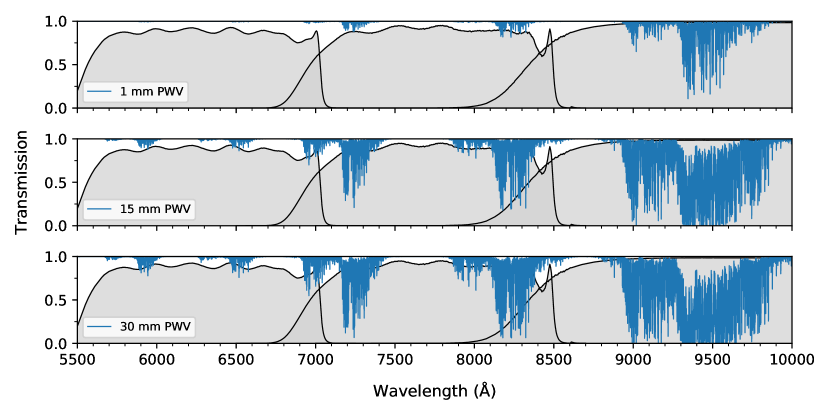
Figure 1: The $r$, $i$ and $z$ band mosaic filters of Kitt Peak National Observatory (grey) compared against the MODTRAN modeled atmospheric transmission function due to precipitable water vapor (blue). Atmospheric transmission functions are shown for an airmass of one and a precipitable water vapor (PWV) column density of $1$ mm (top), $15$ mm (middle), and $30$ mm (bottom). Note that absorption features do not scale linearly with PWV, and some saturate at relatively low column densities.

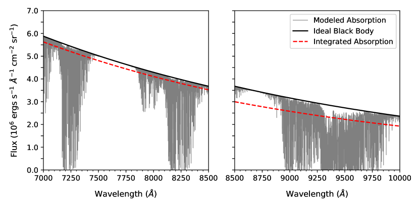
Figure 2: The SED of a blackbody at 8,000 K (black) across the $i$-band (left) and $z$-band (right) ranges. Shown in grey, the modeled atmospheric absorption for a PWV column density of 15 mm is applied to the SED. This is compared to the black body SED scaled using the integrated absorption in each band in red.

2 Background

The atmospheric transmission between $5,500$ and $12,000$ Å is dominated by absorption due to PWV (Figure 1). The strength of PWV absorption lines in observed spectra correlate strongly with measurements of localized PWV column density (Blake & Shaw, 2011). This indicates that PWV measurements can be combined with atmospheric models to provide estimates of the atmospheric transmission at a given date and time. However, accomplishing this requires a source of accurate and readily accessible PWV measurements. Furthermore, since PWV levels can change by over 10% per hour, measurements must be available in close to real time.

By measuring the delay of dual-band GPS signals traveling through the atmosphere, it is possible to determine the PWV column density along the line of sight (see Braun & Hove (2001), Dumont & Zabransky (2001), and Nahmias & Zabransky (2004)). This approach is made even more appealing by the existence of several established GPS networks dedicated to the measurement of geological and meteorological data on the international scale. The SuomiNet project (Ware et al., 2000) is a meteorological initiative that uses data from multiple GPS networks to provide semi-hourly PWV measurements. It currently publishes meteorological data from hundreds of receivers throughout the United States and Central America.

2.1 Effects of PWV on Photometric Calibration

When correcting photometric observations for atmospheric effects, astronomers commonly express atmospheric absorption as a linear function of airmass. In this approach photometric observations are corrected by fitting for a set of extinction coefficients $k^{\prime}$ and $k^{\prime\prime}$ in each band. For example, given an airmass $X$, the observed $i$ and $z$ band magnitudes of a standard star are related to the tabulated, intrinsic magnitudes $z_{0}$ and $i_{0}$ by a set of linear equations

$$\text{z} =\text{z}_{0}+k_{\text{z}}^{\prime}\cdot X+k_{\text{z}}^{\prime\prime}(\text{b}-\text{v})\cdot X$$ (1)

$$\text{i} =\text{i}_{0}+k_{\text{i}}^{\prime}\cdot X+k_{\text{i}}^{\prime\prime}(\text{b}-\text{v})\cdot X$$ (2)

The first order extinction term $k^{\prime}$ accounts for the decrease in a star’s observed flux with airmass. The inclusion of a second order coefficient $k^{\prime\prime}$ accounts for the fact that the observed flux of blue stars decreases faster than red stars as they approach the horizon.

To measure the second-order extinction, observations are taken of a red and blue star over a wide airmass range. The second-order extinction in each band can then be found by fitting for the difference in magnitude between the two stars.

$$\Delta\text{z} =k^{\prime\prime}_{\text{z}}\Delta(\text{b}-\text{v})\cdot X+\Delta\text{z}_{0}$$ (3)

$$\Delta\text{i} =k^{\prime\prime}_{\text{i}}\Delta(\text{b}-\text{v})\cdot X+\Delta\text{i}_{0}$$ (4)

Using the resulting value for $k^{\prime\prime}$, the first order extinction coefficient is then found by fitting Equations 1 and 2. Although this method does account for a first order airmass dependence, it does not directly account for any nonlinear effects. This is to say it does not account for parts of the atmospheric transmission having a nonlinear airmass dependence.

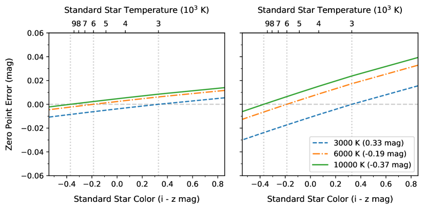
Figure 3: Correcting photometric observations using tabulated values of a standard star introduces residual error in the magnitudes of other stars with different spectral types. The residual error in $z$ band photometric zero point due to absorption by precipitable water vapor is shown for three black bodies at $3,000$ (M type), $6,000$ (G type), and $10,000$ K (A type). Results are shown as a function of the color of the reference star used to calculate the zero point. Error values are shown for a PWV column density of 5 (left) and 30 mm (right).

For a PWV column density at zenith PWV_z, the column density along the line of sight is given by

$$\text{PWV}_{\rm los}=\text{PWV}_{z}\cdot X$$ (5)

However, due to saturation, not all absorption features scale linearly with PWV concentration – some features saturate at relatively low concentrations ($<10$ mm). Thus a linear function of airmass and color is not sufficient to describe the atmospheric transmission from PWV.

Figure 2 details the error introduced by considering PWV absorption averaged over a bandpass versus the actual absorption spectrum. Because atmospheric absorption varies with wavelength, it affects stars differently depending on their spectral type. This means that variations in the spectral types of photometric standards used to correct an image introduce errors in the magnitudes of observed targets. This effect is more pronounced for higher airmass due to the increased PWV along the line of sight, and is an important consideration for KPNO where $\text{PWV}_{z}$ exceeds $20$ mm over 13% of the time.

Demonstrated in Figure 3, when using a type A star to correct cooler G or M type stars, spectral variations between stars used in the atmospheric correction can introduce errors as large as $-0.02$ mag. This error is particularly important when performing high accuracy photometry to 1% or better. An alternative is to correct photometric observations using atmospheric models.

For an atmospheric transmission $T(\lambda)$, the photometric correction for an object with a spectral energy distribution $S(\lambda)$ is given by

$$C=\frac{\int_{\lambda_{i}}^{\lambda_{j}}S(\lambda)\cdot T(\lambda)\,d\lambda}{\int_{\lambda_{i}}^{\lambda_{j}}S(\lambda)\,d\lambda}$$ (6)

where the integration bounds are defined by the wavelength range of the photometric bandpass. Using atmospheric models, measurements of the PWV column density are used to determine $T(\lambda)$ at a given date, time, and airmass. If tabulated values for $S(\lambda)$ are not available, spectral templates are used instead. For example, the SED of a star is well estimated by its color, due to the strong relationship between stellar spectral type and intrinsic color.

2.2 Use of GPS at Kitt Peak

In March of 2015, we installed SuomiNet connected weather station on top of the WIYN 3.5 meter telescope building at Kitt Peak National Observatory. In addition to a GPS receiver, the station includes barometric, temperature, and wind speed sensors. SuomiNet compiles measurements from its affiliated weather stations at thirty minute intervals. These semi-hourly measurements, in addition to the local PWV column density along zenith, are then released publicly on an hourly basis.

In order to prevent equipment damage, the weather station at Kitt Peak is powered down during lightning storms. This creates gaps in the available SuomiNet data for Kitt Peak. Additionally, the barometric sensor was malfunctioning in 2016 from January through March, so we ignore any SuomiNet data published for Kitt Peak during this time period. The sensor has since been repaired, but occasionally records a non-physical drop in pressure. We disregard these measurements by ignoring any meteorological measurements taken for Kitt Peak with a pressure below 775 mbar.

In order to determine the PWV level during periods without SuomiNet data, measurements from other nearby receivers can be used to model the PWV level at Kitt Peak. This model can also be used for times before the Kitt Peak receiver was installed. In addition to data taken at Kitt Peak, the pwv_kpno package uses measurements from four other receivers within a 45 mile radius at varying levels of altitude. This includes receivers located at Amado (AMAZ), Sahuarita (P014), Tucson (SA46), and Sells (SA48) Arizona. The location of these receivers is shown in Figure 4, with SuomiNet measurements for Kitt Peak, Amado, and Sells shown in Figure 5.

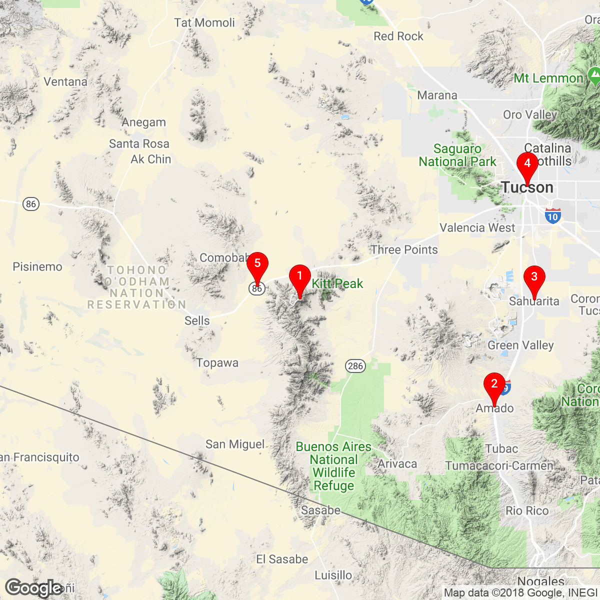
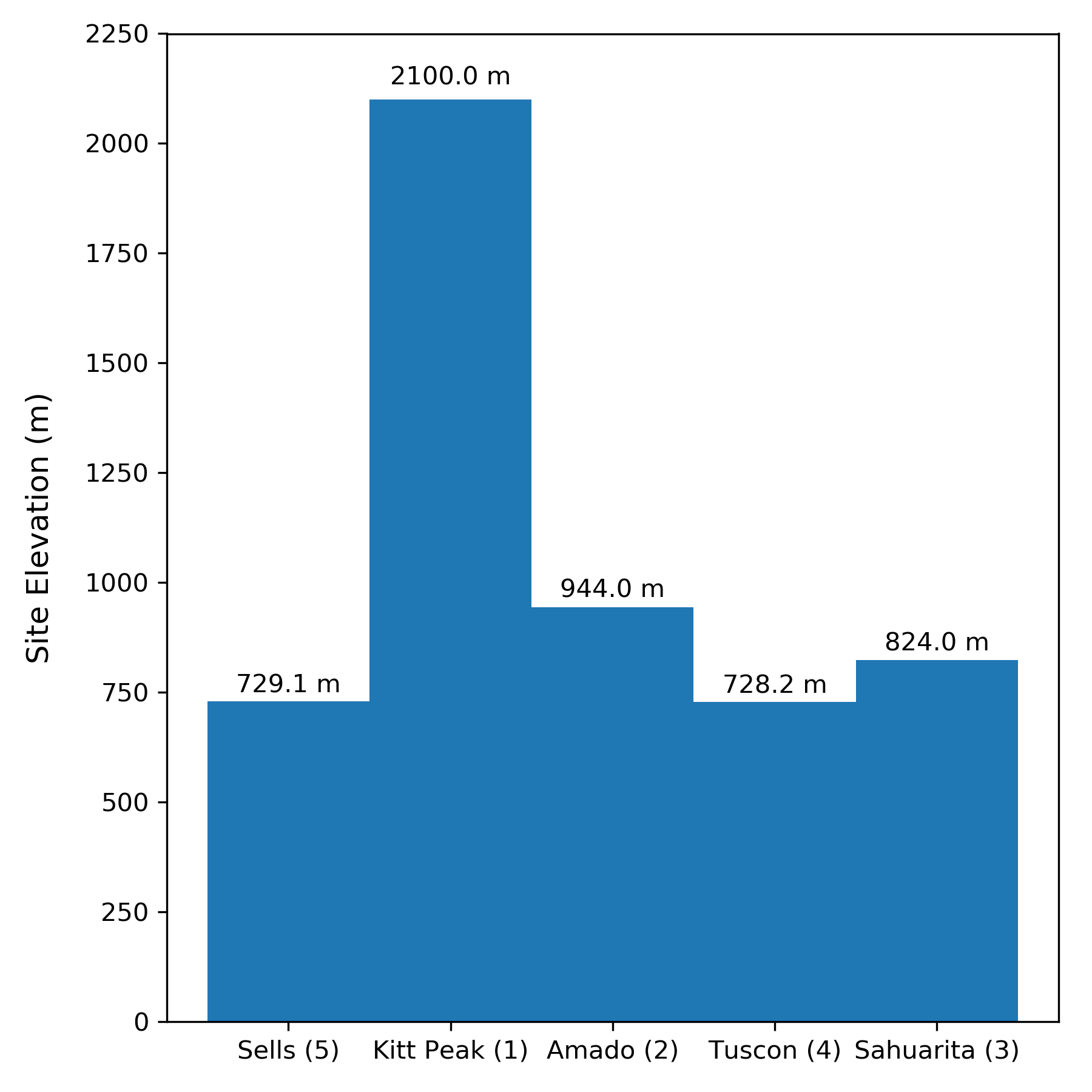
Figure 4: The pwv_kpno package uses PWV measurements for five locations within a 45 mile radius of Kitt Peak. Shown on the left, these locations include Kitt Peak (1), Amado (2), Sahuarita (3), Tucson (4), and Sells (5) Arizona. The elevation of each location is shown on the right.

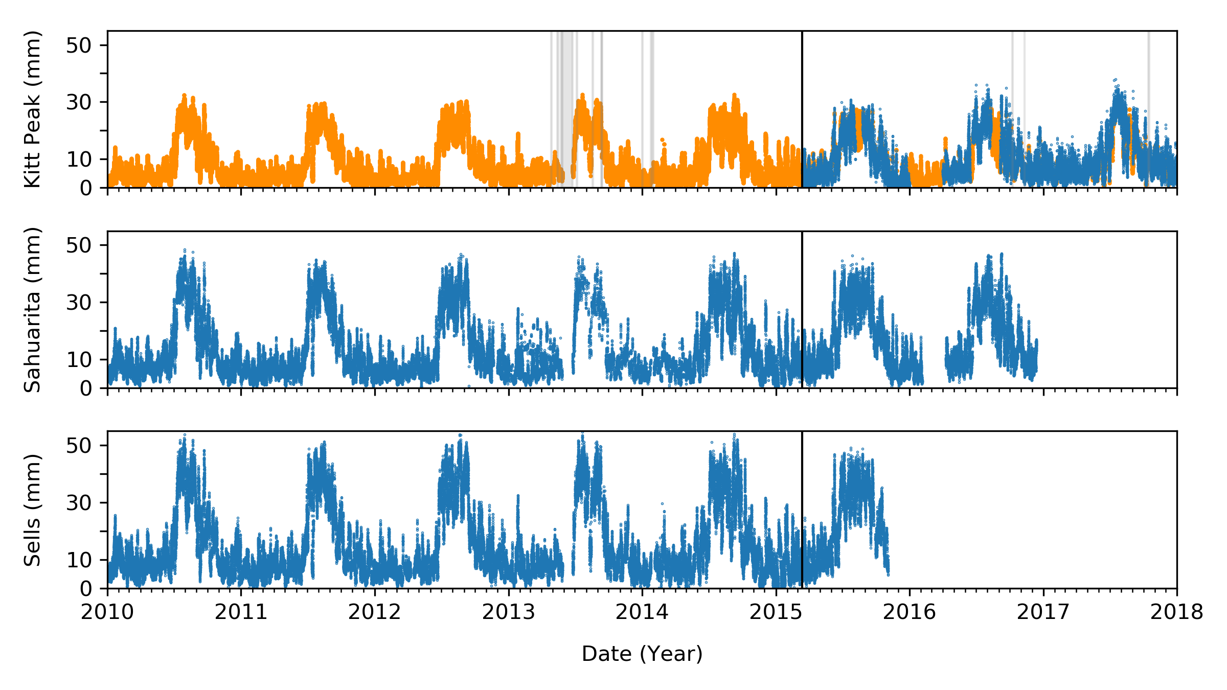
Figure 5: Measurements of precipitable water vapor (PWV) from the SuomiNet project from 2010 onward. From top to bottom, SuomiNet measurements for Kitt Peak National Observatory, Sahuarita AZ, and Sells AZ (Blue). The modeled PWV level at Kitt peak is shown in Orange. Periods of one day or longer where there are no modeled PWV values are shown in the top panel in grey. The geographic proximity of these locations means that the primary difference in PWV between locations is due to differences in altitude. Measurements taken at Kitt Peak National Observatory begin in March of 2015.

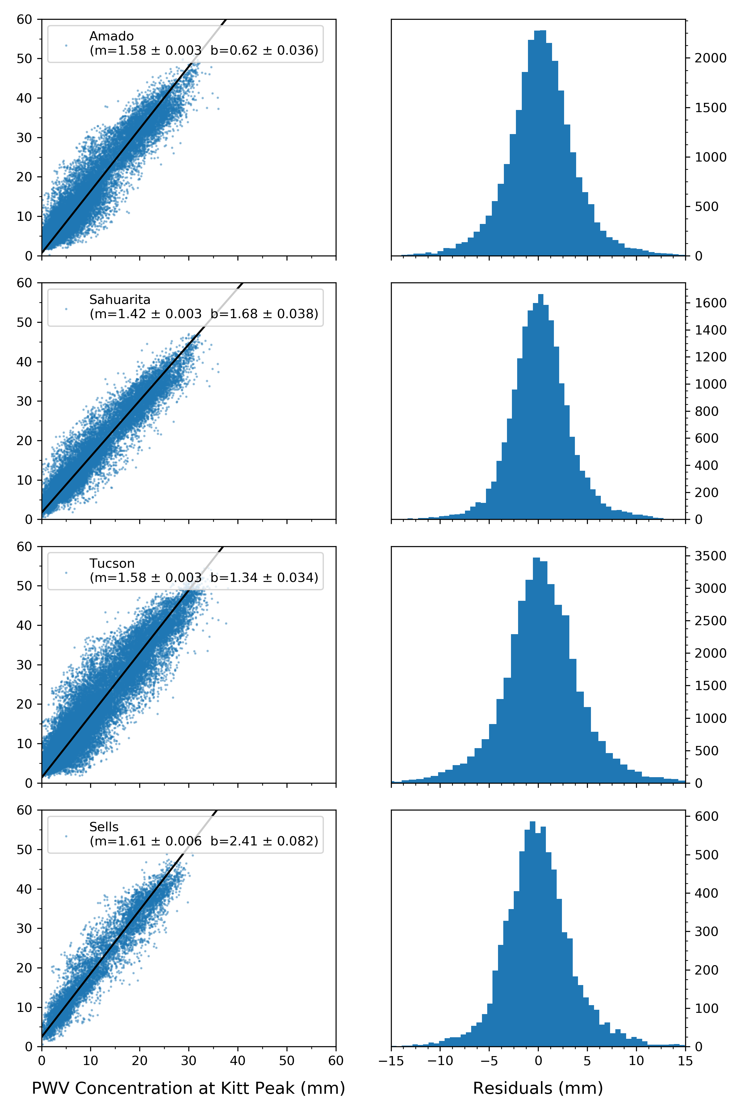
Figure 6: Linear fits to measurements of precipitable water vapor (PWV) column density taken at four different locations versus simultaneous measurements taken at Kitt Peak. Each row corresponds to a different location being compared against Kitt Peak, with measurements shown on the left and binned residuals shown on the right. The slope ($m$) and y-intercept ($b$) is shown for each fit. The correlation in PWV column density between different sites allows the PWV column density at Kitt Peak to be modeled using measurements from other locations.

Note that the PWV level at each location follows the same seasonal trend, but the PWV concentration at Kitt Peak tends to be lower. Since each of the chosen receivers are geographically close together, variations in PWV between Kitt Peak and the four supplementary locations are predominantly caused by differences in altitude. Shown in Figure 6, the PWV level at each location can be related to the PWV level at Kitt Peak by applying a linear fit. Each fit is able to predict the PWV column density at Kitt Peak to a precision of 1 mm plus 10% of the predicted value.

For times when SuomiNet data is unavailable for Kitt Peak, each of the linear fits are used to estimate the PWV column density at Kitt Peak. The resulting estimations are then averaged and used to supplement data taken by the Kitt Peak weather station. This full data set provides a model for the PWV column density at zenith over time.

To determine the PWV column density for a specific date and time, pwv_kpno first determines the concentration along zenith by interpolating from the supplemented PWV data. The PWV column density along the line of site is then calculated using Equation 5. Using this value, pwv_kpno is able to determine the atmospheric transmission using a set of tabulated MODTRAN models.

3 Features and Use of pwv_kpno

The pwv_kpno package provides access to models for the atmospheric transmission due to PWV at any location within the SuomiNet GPS network. However, the package is configured by default to return models for Kitt Peak National Observatory. We here demonstrate the features of pwv_kpno using the default model for Kitt Peak and further discuss modeling custom sites in Section 4

pwv_kpno is registered with the Python Package Index and is compatible with both Python 2.7 and 3.5 through 3.7. Using PWV measurements published by the SuomiNet project, the package is able to determine the atmospheric transmission between $3,000$ and $12,000$ Å. The package also provides methods for the automated retrieval and processing of published SuomiNet data.

3.1 Accessing PWV Data

In order to model the atmospheric transmission for a given date and time, pwv_kpno requires there to be SuomiNet data stored on the user’s local machine. Each package release contains the necessary data to return models for Kitt Peak from 2010 through the end of the previous year. This data is automatically included when installing the package.

Access to tabulated PWV data and modeling of the PWV transmission function is provided by the pwv_atm module. A list of years that have been downloaded from SuomiNet to the user’s local machine can be retrieved using the downloaded_years method.

⬇

>>> from pwv_kpno import pwv_atm

>>> pwv_atm.downloaded_years()

[2010, 2011, 2012, 2013, 2014,

2015, 2016, 2017]

The returned list includes all years for which any amount of data has been downloaded.

In order to update the locally stored data, pwv_kpno can be used to automatically retrieve and processes new data from SuomiNet. This is achieved using the update_models method.

⬇

>>> pwv_atm.update_models()

[2017, 2018]

Here the returned list includes any years for which new data was downloaded. By default, the function will download all published data for any years not currently present on the local machine. In addition, it will also download data for the most recent year that is locally available. This method ensures there are no years with incomplete measurements in the locally available data. If desired, the user can alternatively specify a specific year to download from 2010 onward.

In addition to downloading data for Kitt Peak, the update_models method also downloads measurements taken at the four supplementary locations shown in Figure 4. Each time the method is run, a new set of linear fits is created to describe the PWV concentration at Kitt Peak as a function of the PWV concentration at each supplementary location. These new fits are then used to recreate the entire supplemented PWV model for Kitt Peak. The error in PWV modeled using each of these fits is taken as the standard deviation of that fit’s residuals.

Users can access the locally available SuomiNet data using the measured_pwv method. Results are returned as an Astropy table (Astropy Collaboration et al., 2013) and can be independently filtered by year, month, day, and hour.

⬇

>>> pwv_atm.measured_pwv(

year=2016, month=11, day=14)

date KITT KITT_err P014 ...

UTC mm mm mm ...

---------------- ---- -------- ---- ...

2016-11-14 00:15 4.7 1.025 6.9 ...

2016-11-14 00:45 4.3 1.025 6.7 ...

2016-11-14 01:15 3.9 0.925 6.7 ...

... ... ... ... ...

Excluding the date column, each column is labeled using the SuomiNet identification codes for the GPS receivers.

pwv_kpno also provides access to the modeled PWV column density at Kitt peak via the modeled_pwv method. As in the previous example, these results can also be filtered independently by year, month, day, and hour.

⬇

>>> pwv_atm.modeled_pwv(

year=2016, month=11, day=14)

date pwv pwv_err

UTC mm mm

---------------- --- -------

2016-11-14 00:15 4.7 1.025

2016-11-14 00:45 4.3 1.025

2016-11-14 01:15 3.9 0.925

... ... ...

3.2 Modeling the Atmosphere

For a known PWV column density, the package provides access to the modeled atmospheric transmission via the trans_for_pwv function. This method returns the modeled transmission function as an Astropy table with wavelengths ranging from $3,000$ to $12,000$ Å. For example, given a PWV column density of $13.5$ mm:

⬇

>>> pwv_atm.trans_for_pwv(13.5)

wavelength transmission

Angstrom

---------- ------------

3000.00 0.9999999916

3000.05 0.9999999916

3000.10 0.9999999916

... ...

Atmospheric models can also be accessed for a given datetime and airmass using the function trans_for_date.

⬇

>>> from datetime import datetime

>>> import pytz

>>>

>>> obsv_date = datetime(

>>> year=2013, month=12, day=15,

>>> hour=5, minute=35, tzinfo=pytz.utc)

>>>

>>> pwv_atm.trans_for_date(

date=obsv_date, airmass=1.2)

wavelength transmission transmission_err

Angstrom

---------- ------------ ----------------

3000.00 0.9999999916 1.7305648359e-08

3000.05 0.9999999916 1.7305648359e-08

3000.10 0.9999999916 1.7305648359e-08

... ... ...

If pwv_kpno does not have any supplemented SuomiNet data within a day of the requested datetime, an exception is raised. Both the trans_for_pwv and trans_for_date functions determine the atmospheric transmission by returning a set of MODTRAN transmission models.

3.3 Modeling a Black Body

The blackbody_with_atm module provides functions for modeling the effects of PWV absorption on a black body SED. For example, consider a black body at $8,000$ K under the effects of atmospheric absorption due to $15$ mm of PWV. For a given array of wavelengths in angstroms, the sed method returns the corresponding spectral energy distribution.

⬇

>>> from pwv_kpno import blackbody_with_atm \

>>> as bb_atm

>>>

>>> temp = 8000

>>> wavelength = np.arange(7000, 10000, 100)

>>> pwv = 15

>>>

>>> sed = bb_atm.sed(temp, wavelength, pwv)

The SED from the above example can be seen in Figure 2. If desired, the SED of a black body without atmospheric effects can also be achieved by specifying a PWV column density of zero.

Using the magnitude function, users can determine the magnitude of a black body in a given band. For example, in the $i$ band, which ranges from $7,000$ to $8,500$ Å, the AB magnitude of a black body is found by running

⬇

>>> band = (7000, 8500)

>>> mag = bb_atm.magnitude(temp, band, pwv)

Here the $i$ band is treated as a top-hat function, however, the magnitude function also accepts band as a two dimensional array specifying the wavelength and response function of a real-world band. As in the previous example, the magnitude of a black body without the effects of atmospheric absorption can be found by specifying a PWV level of zero.

4 Modeling Other Locations

By default, pwv_kpno provides models for the PWV transmission function at Kitt Peak National Observatory. However, pwv_kpno also provides atmospheric modeling for user customized locations. Modeling multiple locations is handled by the package_settings module, and allows modeling at any location with a SuomiNet connected GPS receiver.

Each site modeled by pwv_kpno is represented by a unique configuration file. Using the ConfigBuilder class, users can create customized configuration files for any SuomiNet site. As an example, we create a new model for the Cerro Tololo Inter-American Observatory (CTIO) near La Serena, Chile.

⬇

>>> from pwv_kpno.package_settings import \

>>> ConfigBuilder

>>>

>>> new_config = ConfigBuilder(

site_name=’cerro_tololo’,

primary_rec=’CTIO’,

sup_rec=[],

wavelength=custom_wavelengths,

cross_section=custom_cross_sections

)

>>> new_config.save_to_ecsv(

’./cerro_tololo.ecsv’)

Here site_name specifies a unique identifier for the site being modeled, primary_rec is the SuomiNet ID code for the GPS receiver located at the modeled site, and sup_rec is a list of SuomiNet ID codes for nearby receivers used to supplement measurements taken by the primary receiver. Unlike the default model for KPNO, there are no additional receivers near the CTIO and so sup_rec in this example is left empty (the default value). By default, pwv_kpno models use MODTRAN estimates for the wavelength dependent cross section of H₂O from 3,000 to 12,000 Å. The optional wavelength and cross_section arguments allow a user to customize these cross sections in units of Angstroms and cm² respectively.

If desired, users can specify custom data cuts on SuomiNet data used by the package. Data cuts are defined using a 2d dictionary of boundary values. The first key specifies which receiver the data cuts apply to. The second key specifies what values to cut. Following SuomiNet’s naming convention, values that can be cut include PWV  ("PWV"), the PWV error ("PWVerr"), surface pressure ("SrfcPress"), surface temperature ("SrfcTemp"), and relative humidity ("SrfcRH"). For example, if we wanted to ignore measurements taken between two dates, we can specify those dates as UTC timestamps and run

⬇

>>> data_cuts = {’CTIO’:

{’SrfcPress’: [

[time_start, time_end]

]}

}

>>> new_config = ConfigBuilder(

site_name=’cerro_tololo’,

primary_rec=’CTIO’,

data_cuts=data_cuts)

Once a configuration file has been created, it can be permanently added to the locally installed pwv_kpno package by running

⬇

>>> from pwv_kpno.package_settings import \

>>> settings

>>>

>>> settings.import_site_config(

’./cerro_tololo.ecsv’)

This command only needs to be run once, after which pwv_kpno will retain the new model on disk, even in between package updates. The package can then be configured to use the new model by running

⬇

>>> settings.set_site(’cerro_tololo’)

After setting pwv_kpno to a model a specific site, the package will return atmospheric models and PWV data exclusively for that site. It is important to note that this setting is not persistent. When pwv_kpno is first imported into a new environment the package will always default to using the standard model for Kitt Peak, and the above command will have to be rerun.

A complete summary of package settings can be accessed using attributes of the settings object.

⬇

>>> settings.set_site(’kitt_peak’)

>>> print(settings.site_name)

kitt_peak

>>> print(settings.available_sites)

[’kitt_peak’, ’cerro_tololo’]

>>> print(settings.receivers)

[’AZAM’, ’KITT’, ’P014’, ’SA46’, ’SA48’]

>>> print(settings.primary_rec)

KITT

>>> print(settings.supplement_rec)

[’AZAM’, ’P014’, ’SA46’, ’SA48’]

The configuration file for the currently modeled location can be exported by running

⬇

>>> settings.export_site_config(

’./current_site_name.ecsv’)

5 Validation

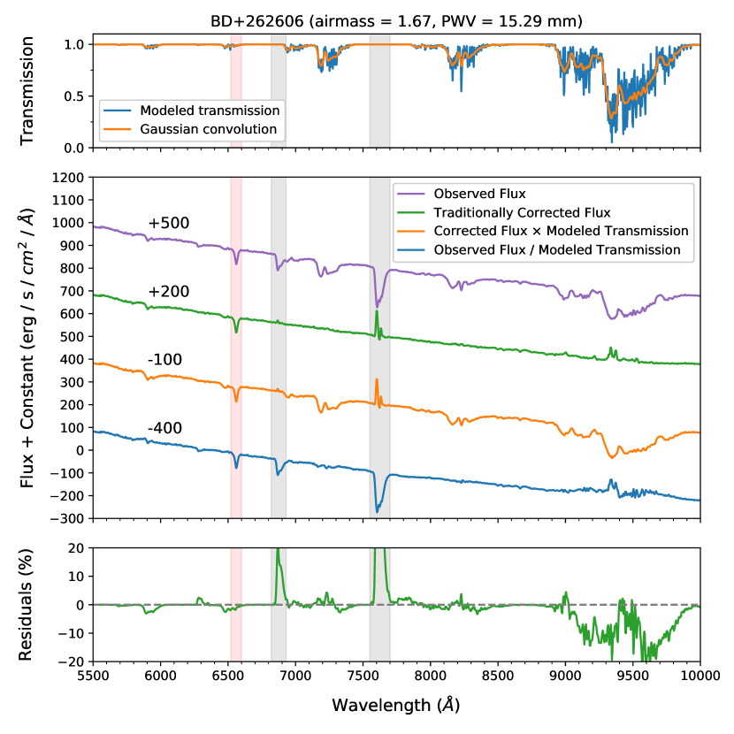
Figure 7: Observations of BD+262606 were taken using the R. C. Spectrograph at Kitt Peak National Observatory. The top panel demonstrates the modeled PWV transmission function at the time of observation (blue) smoothed by a Gaussian kernel (orange). The middle panel shows the observed spectrum (purple) and the spectrum corrected using catalog values (green). These are compared against the catalog corrected spectrum multiplied by the modeled transmission (orange) and the observed spectrum divided by the smoothed transmission (blue). Residuals between the catalog corrected and model corrected spectrum are shown in the bottom panel. H_α lines are highlighted in red and O₂ lines in grey.

From 2010 September 16th through September 20th, an observation run was performed on 18 standard stars using the R.C. spectrograph on the Mayall 4m telescope. To reduce flux loss due to atmospheric dispersion, the spectrograph was configured to use a wide 7″ slit. Observations were recorded between 5,500 and 10,200 Å with an average dispersion of 3.4 Å per pixel. Seeing for all observations varied between 1 and 2″.

As an example, Figure 7 shows the SED of BD+262606 observed at an airmass of 1.67. To flux-calibrate the observed spectrum, low-airmass observations were taken of BD+17 4708 each night. This minimized the introduction of additional telluric effects in the calibrated spectrum. To correct the observed spectrum for atmospheric effects, the absorption in the standard star was scaled to match the airmass of the other observations following the prescription of Wade & Horne (1988).

Note that the atmospheric models used by pwv_kpno do not directly account for the smoothing that occurs in observed spectra due to a spectrograph’s spectral resolution function. As a result, directly dividing the observed spectra and modeled transmission will produce a very high, unphysical flux for wavelengths where the transmission function is saturated. To account for any saturated features, the modeled transmission is first binned to approximately match the observed spectrum’s resolution. The transmission is then smoothed further using a Gaussian kernel.

To correct for atmospheric effects using the pwv_kpno package, the observed spectrum is divided by the smoothed PWV transmission function. We note that the observed spectrum was taken before a GPS receiver was installed at Kitt Peak. This means that no direct PWV measurements are available for the time of observation, and we instead determine the modeled PWV transmission using measurements from GPS receivers on the surrounding desert floor.

In the model-corrected spectrum, the absorption feature at 6,550 Å is an H$\alpha$ line intrinsic to the observed spectrum. Furthermore, the absorption features at 6,875 and 7,650 Å are caused by O₂ absorption. Since pwv_kpno only provides models for the PWV absorption, these two features remain uncorrected. Given that there are no emission lines relative to the continuum, the feature at 9350 Å is categorized as an unidentified artifact from the reduction process.

Corrections for the PWV absorption features agree reasonably well between the catalog and model corrected spectrum. The largest deviations between the corrected spectrum occur redward of 9,000 Å. Some of these deviations can be attributed to cloudy observation conditions, creating large spatial and time variations in the PWV concentration along the line of sight (Querel & Kerber, 2014). However, correcting this feature is also difficult since it is in fact a number of thin, saturated lines that have been blended together. Overall we find that the model struggles to correct the observed spectrum past 9,000 Å, but performed well enough overall to be used to satisfactorily correct photometric observations.

6 Package Demonstration

The pwv_kpno package can be used to correct both spectrographic and photometric observations. As an example, we use the pwv_kpno package to determine the atmospheric correction presented in Figure 7. We also demonstrate how to calculate the photometric correction factor defined in Equation 6 for a black body.

6.1 Correcting Spectra

Spectrographic observations are corrected by dividing observed spectra by the modeled atmospheric transmission function. To account for the spectral resolution function of the observing spectrograph, the modeled transmission is first binned to approximately match the observed spectra’s resolution. Depending on the resolution of the observation, further smoothing can then be performed using a Gaussian kernel. Assume that the observed wavelength and flux values are stored in equal length arrays obs_wavelength and obs_flux respectively. Using the date, time, and airmass of the observation, the binned transmission function is found by running

⬇

>>> import numpy as np

>>>

>>> resolution = 16 # Angstroms

>>> bins = np.arange(min(obs_wavelength),

max(obs_wavelength + 1),

resolution)

>>>

>>> airmass = 1.2

>>> obs_data = datetime(2010, 09, 19, 6, 29

tz_info=pytz.utc)

>>> transm = pwv_atm.trans_for_date(obs_date,

airmass,

bins)

In order to divide the observed spectrum and modeled transmission, we linearly interpolate the binned transmission to the observed wavelength values. We then apply a Gaussian smoothing using an arbitrary standard deviation of 2 Å.

⬇

>>> from scipy.ndimage.filters import \

gaussian_filter

>>>

>>> interp_transm = np.interp(

obs_wavelength,

transm[’wavelength’],

transm[’transmission’])

>>> smoothed_transm = gaussian_filter(

input=interp_transm, sigma=2)

The corrected spectrum is then given as the observed flux divided by the smoothed transmission function on a wavelength by wavelength basis.

⬇

>>> corrected_spec = np.divide(

obs_flux,

smoothed_transm)

6.2 Correcting Photometry

The pwv_kpno package can also be used to correct photometric observations of objects with a known spectral type. To do so, it is necessary to evaluate Equation 6. Note that the product in the numerator $S(\lambda)\cdot T(\lambda)$ represents the SED under the influence of atmospheric effects, while $S(\lambda)$ in the denominator represents the intrinsic SED. For a black body observed in the $i$ band, these values can be found as

⬇

>>> # S(lambda) * T(lambda)

>>> sed_with_atm = bb_atm.sed(

>>> sed_temp, i_band, pwv)

>>>

>>> # S(lambda)

>>> intrinsic_sed = bb_atm.sed(

>>> sed_temp, i_band, 0)

In practice the SED of a photometrically observed object may not be available. In such a case it is sufficient to use spectral templates instead. For example, the SED of a star can be reasonably well parametrized by its observed color.

Using the above results, we evaluate Equation 6 by performing trapezoidal integration with the Numpy package.

⬇

>>> numerator = np.trapz(sed_with_atm, i_band)

>>> denominator = np.trapz(

>>> intrinsic_sed, i_band)

>>>

>>> photo_corr = np.divide(

>>> numerator, denominator)

The corrected photometric flux of the black body is then found by dividing the observed flux by the correction factor photo_corr.

7 Conclusion and Future Work

Atmospheric transmission in the near-infrared is highly dependent on the column density of precipitable water vapor. By measuring the delay in GPS signals through the atmosphere, initiatives such as the SuomiNet project provide accurate water vapor measurements for multiple, international locations. Through the use of atmospheric models, these measurements provide a means for determining the atmospheric transmission due to precipitable water vapor at each location.

Current methods for removing atmospheric effects commonly rely on fitting for a set of extinction coefficients. Unfortunately, this method does not capture the complex nature of the atmospheric transmission function. When calibrating a photometric image, this introduces errors due to spectral variations of the stars used to determine the extinction coefficients. Atmospheric modeling has the potential to provide an alternative that is not influenced by spectral differences.

The Python package pwv_kpno provides models for the atmospheric transmission due to H₂O at user specified sites. For a given date, time, and airmass, the package uses measurements from the SuomiNet project to determine the corresponding PWV column density along the line of sight. By using a set of MODTRAN models, the resulting concentration is then used to determine the PWV transmission function between $3,000$ and $12,000$ Å.

Future work is planned by the primary author to further explore the relationship between PWV measured by geographically separated GPS receivers. Measurements from two, geographically close receivers can be related by a linearly fitting the PWV concentration measured at both sites. However, this linear relationship does not capture the intrinsic scatter of the measured data. Additional models will be explored that take into account simultaneous temperature, pressure, and relative humidity measurements to improve the ability to model the PWV relationship between GPS receivers.

References

- Astropy Collaboration et al. (2013) Astropy Collaboration, Robitaille, T. P., Tollerud, E. J., et al. 2013, A&A, 558, A33
- Berk et al. (2014) Berk, A., Conforti, P., Kennett, R., et al. 2014, Proc. SPIE, 9088, 9088
- Blake & Shaw (2011) Blake, C. H., & Shaw, M. M. 2011, PASP, 123, 1302
- Braun & Hove (2001) Braun, J., & Hove, T. 2001, in Proceedings of the 18th International Technical Meeting of the Satellite Division of The Institute of Navigation
- Burke et al. (2010) Burke, D. L., Axelrod, T., Blondin, S., et al. 2010, The Astrophysical Journal, 720, 811
- Burke et al. (2014) Burke, D. L., Saha, A., Claver, J., et al. 2014, The Astronomical Journal, 147, 19
- Dumont & Zabransky (2001) Dumont, D. M., & Zabransky, J. 2001, in Proceedings of the Eleventh Symposium on Meteorological Observations and Instrumentation, 245–247
- Li et al. (2016) Li, T., DePoy, D. L., Kessler, R., et al. 2016, in Astronomical Society of the Pacific Conference Series, Vol. 503, The Science of Calibration, ed. S. Deustua, S. Allam, D. Tucker, & J. A. Smith, 25
- Nahmias & Zabransky (2004) Nahmias, M. H., & Zabransky, J. 2004, BAMS
- Querel & Kerber (2014) Querel, R. R., & Kerber, F. 2014, in Proc. SPIE, Vol. 9147, Ground-based and Airborne Instrumentation for Astronomy V, 914792
- The Nearby Supernova Factory et al. (2013) The Nearby Supernova Factory, Buton, C., Copin, Y., et al. 2013, A&A, 549, A8
- Vacca et al. (2003) Vacca, W. D., Cushing, M. C., & Rayner, J. T. 2003, PASP, 115, 389
- Wade & Horne (1988) Wade, R. A., & Horne, K. 1988, ApJ, 324, 411
- Ware et al. (2000) Ware, R. H., Fulker, D. W., Stein, S. A., et al. 2000, Bulletin of the American Meteorological Society, 81, 677