Abstract

We consider a model of an artificial neural network that uses quantum-mechanical particles in a two-humped potential as a neuron. To simulate such a quantum-mechanical system the Monte-Carlo integration method is used. A form of the self-potential of a particle and two potentials (exciting and inhibiting) interaction are proposed. The possibility of implementing the simplest logical elements, (such as AND, OR and NOT) based on introduced quantum particles is shown. Further we show implementation of a simplest convolutional network. Finally we construct a network that recognizes handwritten symbols, which shows that in the case of simple architectures, it is possible to transfer weights from a classical network to a quantum one.

1 Introduction

The modern development of various fields of science and technology strongly depends on progress in computer science. Such progress can be associated with the implementation of new technologies of computing systems as well as with new computational algorithms. The two main tendencies in the development of the computer science are quantum computing and artificial intelligence.

The logical elements of computer processors become smaller and smaller with time. Today the technology gives us the possibility to produce such elements very close to quantum limit where quantum fluctuations became more and more essential. On the one hand, the quantum nature of such elements can lead to the crisis of the classical computing technique, but on the another hand the quantum properties of the elements can be used for realization of quantum calculation algorithms.

Another main tendency in modern development of computer science is the artificial intelligence. Artificial neural networks are the computing systems inspired by the biological neural networks and consist of the set of connected calculation nodes (artificial neurons). Like in the brain the connections between such nodes transmit the signals from one node to another. The parameters of such connections depend on weights. By changing of these weights one can modify the transport of the signals in the neural network. The learning procedure of the neural network just consists in the tuning of these weights. There are many computing problems can be solved by using of artificial neural networks like images [1] and speech [2] recognitions, machine translation [3] and so on.

Is it possible to combine these two concepts and propose quantum system which would work as a neural network? How small such system could be? In our work we try to find the answer on these questions.

The integrate-and-fire neuron is one of the simplest model of neuron. In framework of this simplification the neuron’s function is to integrate of external activity of another neurons and produces a spike if this integrated external activity reaches some threshold value. In such cases the neuron excitation is transmitted to other neurons in the network. The quantum objects are stochastic by nature and we can say only about probability of excitation of our quantum neurons. However, the quantum nature of our neural network will not prevent us from implementation of all basic functions of the neural networks. Moreover, the analogy with quantum computers allows us to hope that this quantum nature will significantly improve the functionality of such a network.

The main function of the neuron (classical and quantum) should be the production of spikes or bursts of activity. In our model we propose a soliton solutions of a quantum system as an analog of such spike. The example the soliton is a well-known kink solution (or instantons) [4] which is connected with spontaneous tunnelling processes between vacua in the model of the quantum particle in the two-humped potential. These processes are associated with bursts of action which can be used as an analog of spikes. If we organize connections between quantum neurons so that a kink in one of the quantum neurons would produced a kink in another one then the activity that has arisen in one part of the network will spread to other parts of our network and our quantum neural network will start to work.

Our work is organized as follows. First, we discuss the general principles of constructing a quantum neural network. As an example of the simplest implementation, basic logic elements are considered. Next, we consider a more complicated problem of recognizing the vertical line. At last part, we show how a quantum network can be applied to digital numbers recognition problem and some principles of quantum neural network learning are also discussed.

2 Formulation of problem

2.1 Quantum neurons (Q-neuron)

Figure 1: Instanton action density. $N_{t}$ is the index of a time slice.

Consider a model of a quantum mechanical system organized as a neural network. A neural network consists of nodes (neurons) and connections between them (axons). The role of neurons in the model will be played by quantum-mechanical particles $\hat{p}_{i}$, evolving under the influence of potential

$$\hat{H}_{i}=\frac{1}{2}\hat{p}_{i}^{2}+V_{0}\left(\hat{\varphi}_{i}\right).$$ (1)

The role of connections between neurons will be played by the interaction potential:

$$V_{int}=V_{int}\left(\hat{\varphi}_{i},\hat{\varphi}_{j}\right).$$ (2)

Thus, the total Hamiltonian of the system will be following

$$\hat{H}=\sum_{i}\left(\frac{1}{2}\hat{p}_{i}^{2}+V_{0}(\hat{\varphi}_{i})\right)+\sum_{i>j}V_{int}(\hat{\varphi}_{i},\hat{\varphi}_{j}).\\$$ (3)

Since in the general case we need to deal with sufficiently complex quantum-mechanical systems, to describe their properties we will be using the well-known path integral Monte Carlo formalism. In Euclidean time, the statistical sum of the system has the form

$$Z=\int\prod_{i}\mathcal{D}\varphi_{i}\left(\tau\right)\exp(-S(\varphi_{i}(\tau))),\varphi_{i}(0)=\varphi_{i}(T),$$ (4)

where $\varphi_{i}(\tau)$ – is the Euclidean path of i-th particle, $\tau\in\left[0,T\right]$ – Euclidean time, and $S(\varphi_{i})$ – classical action:

$$S=\int_{0}^{T}d\tau\left[\sum_{i}\left(\frac{1}{2}\dot{\varphi}_{i}^{2}+V_{0}(\varphi_{i})\right)+\sum_{i>j}V_{int}(\varphi_{i},\varphi_{j})\right].$$ (5)

The observables in such formalism are calculated as

$$\braket{\mathcal{O}(\varphi_{1},...,\varphi_{i})}=\frac{1}{Z}\int\prod_{i}\mathcal{D}\varphi_{i}(\tau)\mathcal{O}(\varphi_{1},...,\varphi_{i})\exp(-S(\varphi_{i})).$$ (6)

We now choose the intrinsic potential of the neuron $V_{0}(\varphi_{i})$. The main function of a neuron is to generate spikes. Suitable feature can be provided by a particle in the W-potential:

$$V_{0}(\varphi_{i})=\frac{\Lambda}{4}\left(\varphi^{2}-1\right)^{2}.$$ (7)

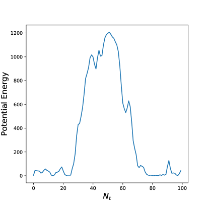
A typical quantum-mechanical behavior of such a particle is a vacuum fluctuation and a rapid change of the vacuum state (instanton). The instantons are accompanied by a peak of the action density (Fig. 1), similar to the potential of the spike of a biological neuron.

The explicit form of interaction between neurons will be introduced in the next Section.

2.2 Methods of solution

The operation of the network is based on the propagation of activity from the input nodes (sensors) to the output ones. As already noted, the network can consist of many nodes. To study such a complex quantum system, it is natural to apply the Monte Carlo method[5]. The idea of the method is to use the Markov process, to generate paths of particles $\varphi_{i}$ with a statistical weight proportional to $\exp(-S(\varphi_{i}))$.

In our work we use the multilevel algorithm of Metropolis. The introduction of several levels of the algorithm is caused by the need to suppress autocorrelations and makes it possible to improve the computational efficiency.

3 Excitatory and inhibitory connections of neurons and logical elements

3.1 Single neuron

Figure 2: Free neuron path. Neuron does not exhibit a spike (i.e. does not move from one vacuum to another) unless excited.

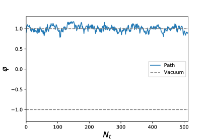
We start the consideration of our model with a case of a single neuron. As we have already said, an artificial neuron in our case will be represented by a particle located in a two-humped potential. A spike or a single act of activity of such a neuron is the transition of a particle from one vacuum to another. The Lagrangian of such a system is written as:

$$\mathcal{L}_{0}=\frac{1}{2}\dot{\varphi}^{2}+\frac{\Lambda}{4}\left(\varphi^{2}-1\right)^{2}.$$ (8)

As can be seen from the Lagrangian, the minima of the potential energy of such a particle are at the points $1$ and $-1$. The value of the classical action for the transition from one minimum to another is [4]

$$S_{cl}=\frac{2\sqrt{2\Lambda}}{3}.$$ (9)

This value will be necessary in order to select suitable $\Lambda$. First, we want the fluctuations of our particle around the energy minima to be small. Secondly, we want to minimize the number of spontaneous transitions from one state to another. In our case, the optimal parameters appeared to be: $\Lambda=5000$. Parameters of the Metropolis algorithm were chosen as follows: time (inverse temperature) $T=0.7$, number of time grid nodes $N_{t}=512$. To suppress autocorrelations, we use the thermalization length in $2\cdot 10^{6}$ iterations. Finally, note that for the initialization of the path we use the saw path of 0’s and 1’s: $\varphi_{init}=i\bmod 2$ where $i\in[0,512]\cap\mathbb{Z}$ is the number of corresponding time grid node. A typical thermalized path is presented in the Fig. 2.

3.2 Two neurons

We now turn to the case of two interacting neurons. We want a spike in one of them to cause a spike in the other, but spikes in the second one should not affect the first one. This means that the interaction Lagrangian of such neurons must be asymmetric (we call such a Lagrangian excitatory):

$$\mathcal{L}_{int}=\varepsilon_{exc}\varphi_{1}^{2}\left(\varphi_{2}^{2}-1\right)^{2},$$ (10)

where $\varepsilon_{exc}$ is the connection strength. If $\varphi_{1}$ is in the vacuum, then there is no impact on $\varphi_{2}$. But, if $\varphi_{1}$ experiences a spike, then $\varphi_{2}$ also tends to have a spike. Thus the activity is spreading from one node to another.

Figure 3: Interaction potential for transmission of spikes from neuron $\varphi_{2}$ to $\varphi_{1}$.

Figure 4: Potential energy of affected neuron (solid) tend to resemble one of input neuron (dashed).

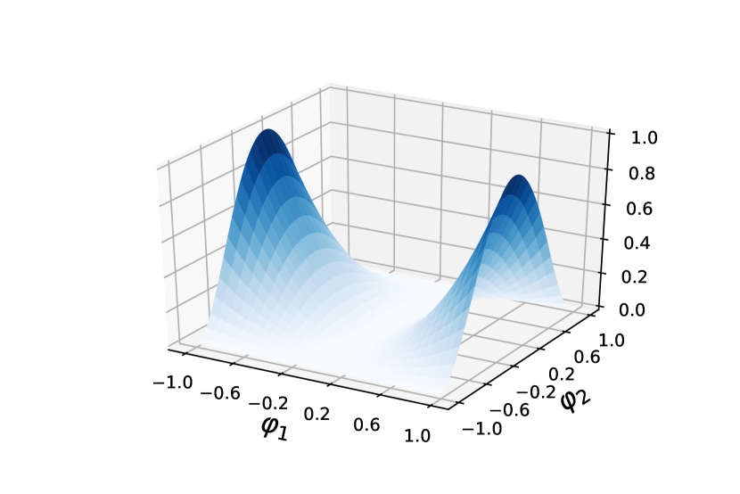
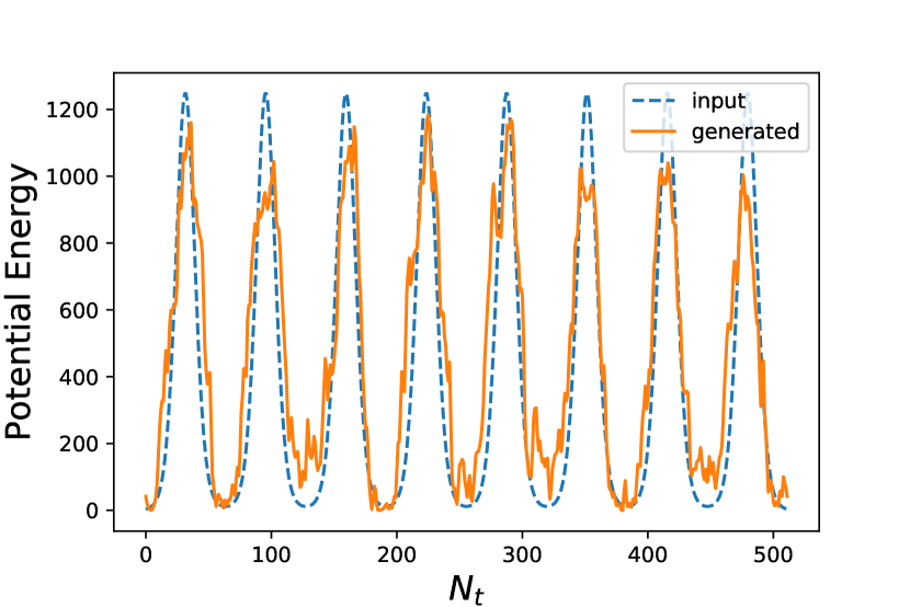
The plot of the potential of such interaction is shown in Fig. 4. Axis $\varphi_{2}$ is related to the excitatory neuron and $\varphi_{1}$ corresponds to affected one.

For representing input information, we are going to use input neurons. Each input neuron can be either passive (make no affect at all so may be discarded) or be active. Active input neurons have fixed path (unlike simulated neurons which path evolves during simulation) which consists of classical kink solutions. Potential energy of such an input neuron is depicted in Fig. 4 (dashed line). Each peak of potential energy corresponds to the kink. Solid line represents the potential energy of the single neuron affected by the input neuron.

We introduce activity of any simulated neuron as ratio of integral potential energy of that neuron to input one (e.g. activity of neuron which never leave vacuum will be 0 and activity of a neuron which path replicates path of input neuron will be 1). In order to investigate different schemes we will inspect plots of activity at some neuron as function of connection strengths $\varepsilon_{exc}$.

Figure 5: Activity of output neuron grows as function of connection strength.

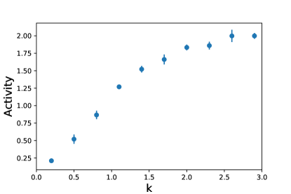
In order to study different configurations of neurons we introduce modulating factor $k$. Once we choose appropriate parameter $\hat{\varepsilon}$ for every connection, we multiply each of them by this factor to obtain new connection strengths $\varepsilon=k\cdot\hat{\varepsilon}$ and than plot activity of neuron of interest as a function of single parameter $k$.

It was found that $\varepsilon_{exc}$ can take it’s values in the range from $3000$ to $8000$ (Fig. 5). In the case of too small $\varepsilon_{exc}$ neurons almost do not interact and if $\varepsilon_{exc}$ is too large, their own potentials become insignificant in comparison with the interaction, which leads to an undesirable delay of the neuron in the state of $\varphi=0$. Plot for $\varepsilon_{exc}=6000$ is presented in Fig. 4.

In the simulation presented in Fig. 4 the activity of output neuron appeared to be 0.92.

Figure 6: Input neuron excites 3 simulated neurons placed in a row.

Figure 7: Activity of output neuron (neuron 3) as a function on connection strength. $\varepsilon_{1}=k\cdot 1.5\cdot 10^{4},\varepsilon_{2}=k\cdot 1.0\cdot 10^{4},\varepsilon_{3}=k\cdot 0.5\cdot 10^{4}$. (see Fig. 6)

Figure 8: Activity of output neuron as a function of $\Lambda$. (see Fig. 6)

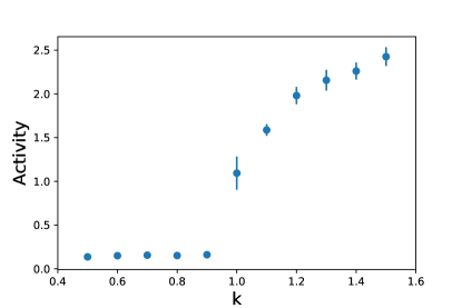
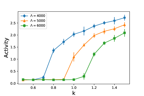
It is possible to transmit an impulse through a line several simulated neurons. Consider the line of three simulated neurons (Fig. 6, 7). In this case we choose $\varepsilon_{1}=k\cdot 1.5\cdot 10^{4},\varepsilon_{2}=k\cdot 1.0\cdot 10^{4},\varepsilon_{3}=k\cdot 0.5\cdot 10^{4}$. As can be seen from Fig. 7, for small values of the connection strength $\varepsilon$, the spikes do not pass through the chain of neurons, but if $\varepsilon$ reaches some critical value, the chain becomes transparent for spikes. This effect allows us to control the transparency of the neural network by the slight changing of the connection strength $\varepsilon$. Thus, by controlling the connection strength, we can realize complex logical connections within our neural network.

The dependence of out neuron activity on the parameter $\Lambda$ is shown in Fig. 8. From this figure it can be seen that the critical value of the connection strength $\varepsilon$ depends on the $\Lambda$. Obviously, such dependence of the critical value of $\varepsilon$ is associated with an increasing of kink’s action (9).

3.3 Logical elements

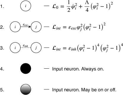
We can now turn to the construction of logical elements. In this subsection we construct from just introduced neurons the simplest logical elements, such as AND, NOT, OR and XOR. In order to simplify presentation, we will use the schematic notation for network elements (Fig. 9).

Figure 9: Schematic signs used to simplify presentation. 1. Contribution to the Lagrangian from neuron with index $i$. 2. Contribution of excitatory connection from neuron $i$ to $j$. 3. Contribution of inhibiting connection between neuron $i$ to $j$. 4. Input neuron that always active. Its path does not change as simulation goes. 5. Input neuron that can be either in active or passive mode. Depending on whether this neuron is active the network should behave in different way.

3.3.1 Logical AND

Logical AND appears to be the simplest element in it’s construction. A neuron connected by a logical AND with some set of other neurons should experience a spike when all of the neurons it connected with experience a spike.

To implement such a behavior, it is necessary to connect the neuron by excitatory potential with those neurons whose signals we need to logically multiply. It is necessary to choose $\varepsilon_{exc}$ sufficiently small so our output neuron activates only when all of its inputs are active, and is passive if at least one of input neuron is passive.

Figure 10: Scheme implementing logical AND. Neurons 1 and 2 consume input and neuron 3 outputs information.

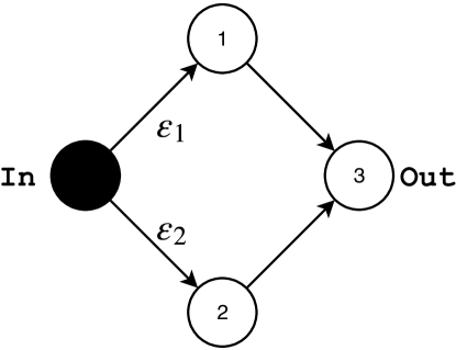
We demonstrate the operation of such construction in the following example. In the Fig. 10 the scheme of such network is presented. A solid circle indicates the active input neuron. Circles with numbers are simulated neurons. The arrows show the connections, and the number next to the arrow corresponds to $\varepsilon_{exc}$.

Figure 11: The AND case (Fig. 10). Activity of output neuron is nonlinear as function of connection strength scale $k$. It resembles a smoothed version of step function expected for discrete case.

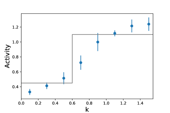
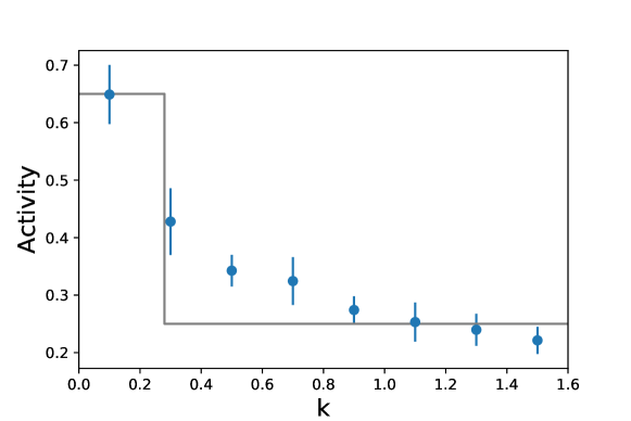
We are interested in two different modes of such a system: $\varepsilon_{1}=\varepsilon_{2}=\hat{\varepsilon}=8000$ (On AND On should result in On output) and $\varepsilon_{1}=0,\varepsilon_{2}=\hat{\varepsilon}$ (Off AND On should result in Off output). We choose $\varepsilon_{1}=\hat{\varepsilon},\varepsilon_{2}=k\hat{\varepsilon}$. The plot of the activity of output neuron as function of $k$ is shown in Fig. 11. One may recognize step function in the output pattern.

3.3.2 Logical NOT

Up to this point, we only caused spikes in the neurons, but to implement arbitrary logic we need to be able to suppress them. For this purpose, we introduce a logical NOT. We add one more type of connection, which we call an inhibiting one. Two neurons connected by such a connection should not spike simultaneously. The interaction Lagrangian that implements the proposed behavior can be written as follows:

$$\mathcal{L}_{int}=\varepsilon_{inh}\left(\varphi_{1}^{2}-1\right)^{4}\left(\varphi_{2}^{2}-1\right)^{4}.$$ (11)

Figure 12: Inhibiting potential that is used to prevent simultaneous spike of $\varphi_{1}$ and $\varphi_{2}$.

Figure 13: Scheme implementing logical NOT. Due to $\varepsilon_{inh}$ only one of output neurons can be active at the same moment.

Figure 14: The NOT case (Fig. 13). The activity of output neuron 2. Neuron with weaker connection to input one is inhibited by another neuron as inhibiting connection becomes stronger.

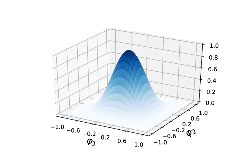
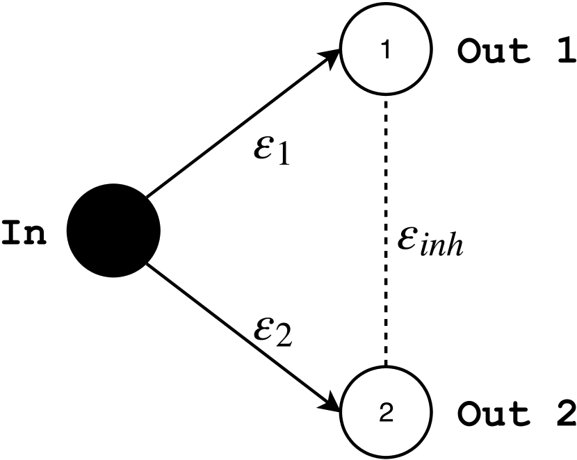
The plot of the corresponding potential is shown in Fig. 13. Apparently, such interaction has effect only if both neurons experience a spike.

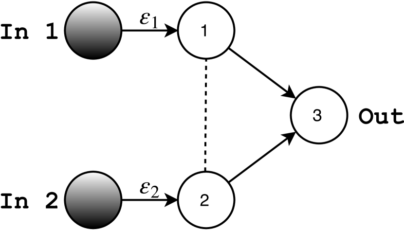
To demonstrate the operation of such a connection, consider the scheme depicted in Fig. 13. Here the dashed line shows the inhibiting connection. We set $\varepsilon_{1}>\varepsilon_{2}$. Activity of neuron 2 as function of $\varepsilon_{inh}$ is presented in Fig. 14, where $\varepsilon_{inh}=50000k$. As one can see, when $\varepsilon_{inh}\approx 0$, neuron 2 is active but as $\varepsilon_{inh}$ grows, neuron 2 becomes inhibited by the neuron 1.

3.3.3 Logical OR

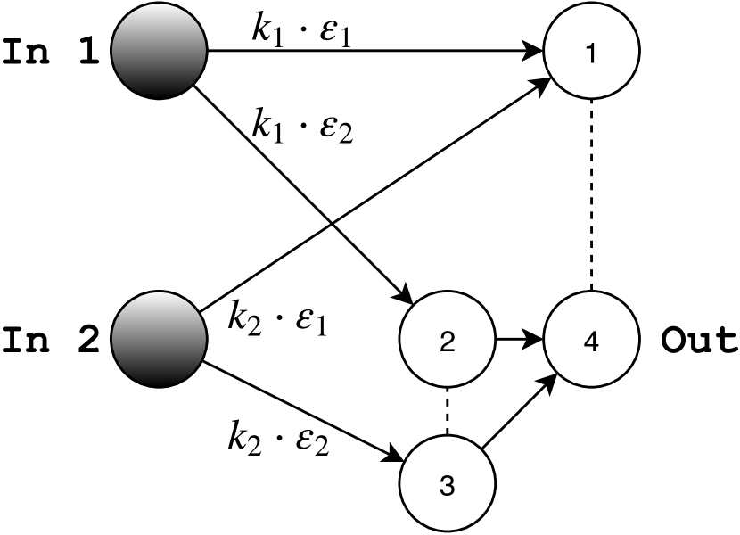
We are now to consider the logical OR. Disjunction in our case works as follows: an output neuron connected to some set of other neurons, activates when at least one of the input neurons is active. At a first glance it may seem that it is enough to simply connect the neurons with an ordinary exciting connection with sufficient $\varepsilon_{exc}$ in order to implement such a behavior. Unfortunately, this can not be done: as we already noted earlier, appropriate value of $\varepsilon_{exc}$ is restricted from above which will be violated if all the exciting neurons experience a spike at the same time (effective $\varepsilon_{exc}$ will be the sum of all the $\varepsilon_{exc}$’s of active neurons). An appropriate construction is depicted in Fig. 16. It turns out that we should use intermediate neurons that inhibit each other in such a way that only one of them can be active at the same time. Only after that they can be connected to the output neuron. Since the intermediate neurons become active one by one, the output neuron will never be overwhelmed.

Figure 15: The logical OR implementation scheme.

Figure 16: The logical XOR implementation scheme. $\varepsilon_{1}=3000,\varepsilon_{2}=10000.$

Figure 17: The OR case (Fig. 16). The activity of output neuron 3. Output neuron is only affected by strongest input neuron. When $k=1$ both input neurons are equal.

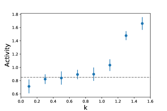
Again, consider two different modes of operation: $\varepsilon_{1}=\varepsilon_{2}=\hat{\varepsilon}=8000$ (On OR On should result in On) and $\varepsilon_{1}=0,\varepsilon_{2}=\hat{\varepsilon}$ (Off OR On should also result in On). We choose $\varepsilon_{1}=\hat{\varepsilon},\varepsilon_{2}=k\hat{\varepsilon}$ and plot the dependency of the activity of output neuron on $k$ (Fig. 17). Note that one may treat $OR(a,b)$ as $max(a,b)$: $\forall a,b\in\{0,1\}:max(a,b)=OR(a,b)$. And this is what we see on the plot. While $k<1$ the activity of output neuron does not change ($activity(max(\hat{\varepsilon},k\hat{\varepsilon}))\overset{k<1}{=}activity(\hat{\varepsilon})$) and as $k$ becomes bigger than 1 the activity of output neuron also increases.

3.3.4 An example of construction of logical XOR

We already have elements from which we can build arbitrary logic, but before we move on to more complex schemes, we will make sure that those elements can operate together. To do this, we construct from them a slightly more complex element - the exclusive or. The idea of its operation is quite expected: the output neuron should be active if and only if one of the input neurons is active.

We achieve this by means of the scheme depicted in Fig. 16. Operation of the scheme is very simple: neuron 4 is active when at least one of the input neurons is active. But if both are active, neuron 1 will inhibit its activity.

Figure 18: The XOR case (Fig. 16). Activity of output neuron resembles smoothed step function: it is high if one of the input neurons is effectively turned off by damping its connections with small factor of $k$ and low if both neurons are active.

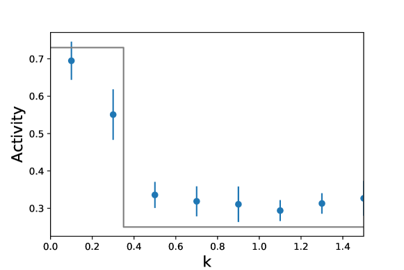
Let’s see how output neuron (4-th) react to change in input’s $\varepsilon$. Activity of output neuron as function of $k_{1}$ is shown in Fig. 18. If first neuron is off ($k_{1}=0$) then activation of second neuron leads to increase of activity of output neuron. But if first input neuron is active then activation of second neuron leads to decrease of activity of output neuron.

4 Applications of the model

4.1 Convolutional model for vertical line detection

We now move on to a more complex system – first neural network. We are to consider convolutional neural network [1] popularized by Krizhevsky et al. [6].

Basic operation principles of such a network is as follows: the input is an image, each pixel depending on its color can be represented by neuron with varying activity. A convolution operation with some predetermined kernel is applied to the input image. In our case the kernel is a matrix of size $3\times 3$, its elements can represent $\varepsilon_{exc}$ or $\varepsilon_{inh}$. We apply element-wise this matrix to the input image in every possible position. Depending on the position of the application of the kernel, the neurons of the input layer will be connected to some neuron of the second layer.

The simples application of convolution model is vertical line detection problem. Let us put the problem as follows: at the input we have a picture of size $4\times 4$ pixels. The network is supposed to be able to detect a vertical line in this picture. If there is something else besides the vertical line on the input image, then the network should not react to such input. Since the input layer has dimension $4\times 4$ second one should be of size $2\times 2$ and third layer is represented by a single neuron. We connect all neurons of the second layer to the neuron of third one using $\varepsilon_{exc}=4000$. To connect the first and second layers we will use the following kernels:

$$K_{exc}=\begin{pmatrix}0&1&0\\ 0&1&0\\ 0&1&0\end{pmatrix}\times 2000,K_{inh}=\begin{pmatrix}1&0&1\\ 1&0&1\\ 1&0&1\end{pmatrix}\times 15000.$$ (12)

Figure 19: Proposed architecture of a convolutional network.

Figure 20: Activity of output neuron is high in case if input resembles vertical line and low otherwise.

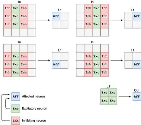
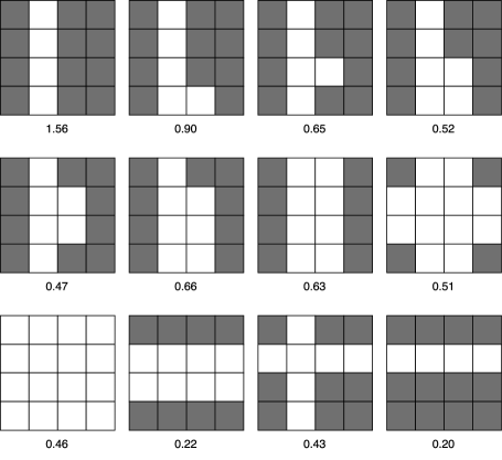
In Fig. 20 the general scheme of proposed network, consisting of three layers is depicted, and in Fig. 20 different input images and network reactions to them are shown. As one can see, the network performs well and finds a vertical line.

In real problems, the input image will have a much larger dimension, which will lead to the need of increasing the number of layers that will combine the different kernels, which will represent increasingly complex images. Simulation of such a network can take a long time, but it will not have any fundamentally new parts. Thus, we can conclude that the proposed model can be used for implementing a convolutional neural networks.

4.2 Digit recognition

Figure 21: Sample digits from MNIST database.

Figure 22: Weights learned by classical neural net for every output (0 to 9).

The last considered example is the use of our network for the recognition of handwritten digits. The problem is formulated as follows: as the input there is an grayscale image of the digit of the size $28\times 28$ pixels, each of which is represented by an input neuron. At the output, there are 10 neurons, each of which detects corresponding digit. So our network is the map $\mathbb{R}^{28\times 28}\rightarrow\mathbb{R}^{10}$.

We we start with solving this problem using multinomial logistic regression. Consider $X\in\mathbb{R}^{N\times M}$ where $N$ is the number of images in training set and $M=28^{2}=784$ is the size of an image. So $X_{ij}$ represents the brightness of $j$-th pixel in $i$-th image. We then map each image into 10 scores corresponding to numbers using $W\in\mathbb{R}^{M\times 10}$ via matrix multiplication: $S=XW$. So $S_{ij}$ corresponds to score of $i$-th image treated as $j$-th number. In order to obtain probabilities we apply softmax function to scores:

$$p_{ij}=\frac{exp(S_{ij})}{\sum_{j=0}^{9}\left(exp(S_{ij})\right)}.$$ (13)

We can estimate $W$ by minimizing loss function:

$$L=-\frac{1}{N}\sum_{i=0}^{N-1}\sum_{j=0}^{9}ln(p_{ij})\delta^{j}_{c(i)}$$ (14)

where $c(i)$ is the digit with index $i$ in our dataset. So $\delta^{j}_{c(i)}$ is 1 for $j$ corresponding to correct digit and 0 otherwise. We are going to use $W$ as connection strengths ($\varepsilon_{exc}$) in our network so they should not be negative. So we add term to loss function (14) penalizing negative weights:

$$L=-\frac{1}{N}\sum_{i=0}^{N-1}\sum_{j=0}^{9}ln(p_{ij})\delta^{j}_{c(i)}+\lambda\sum_{i=0}^{M-1}\sum_{j=0}^{9}max(-W_{ij},0),\lambda\gg 1.$$ (15)

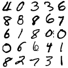
To train a classical network, we need many examples of images of handwritten figures, which should already be properly marked. We will use the MNIST database[7] (Fig. 22). It consists of 60,000 training samples and 10,000 test samples. Resulting weights $W$ are shown in Fig. 22. The accuracy of recognition of the classical network appeared to be $91\%$ on the test set.

We can now use $W$ as connection matrix for $\varepsilon_{exc}$ connecting input and output layers of our quantum net. We treat activity of each neuron as its ’vote’ for corresponding number. We then normalize activities to obtain values that sum to 1 using softmax function.

The Lagrangian of the recognition system is written as follows:

$$\mathcal{L}_{0}=\sum_{i=0}^{784}\left[\frac{1}{2}\dot{\hat{\psi}}_{i}^{2}+\frac{\Lambda}{4}\left(\hat{\psi}_{i}^{2}-1\right)^{2}\right]+\sum_{j=0}^{10}\left[\frac{1}{2}\dot{\varphi}_{j}^{2}+\frac{\Lambda}{4}\left(\varphi_{j}^{2}-1\right)^{2}\right],$$ (16)

$$\begin{split}\mathcal{L}=\mathcal{L}_{0}&+\sum_{i=0}^{784}\sum_{j=0}^{10}k\hat{\varepsilon}_{ij}\varphi_{j}^{2}\left(\hat{\psi}_{i}^{2}-1\right)^{2}+\\ &+10^{-17}\sum_{k>j}^{10}\sum_{j=0}^{10}\left(\varphi_{j}^{2}-1\right)^{4}\left(\varphi_{k}^{2}-1\right)^{4},\end{split}$$ (17)

where $\hat{\psi}_{i}$ represents the path of neurons corresponding input image. $\varphi_{j}$ is the coordinates of the output neurons. $\varepsilon_{ij}$ is the connection strengths of the input and output layers, we transfer them from the already trained classical network and normalize to be in $[0,1]$ according to (18).

$$\hat{\varepsilon}_{ij}=\frac{W_{ij}-min(W)}{max(W_{ij}-min(W))}.$$ (18)

Finally $k=1000$. Note that the first sum in $\mathcal{L}_{0}$ can be discarded, since it is a constant and does not change in the modelling process.

Our input image is grayscale which means that its parameters may have any value in $[0,1]$ but up to this moment we only had binary input neurons (active and passive). We should somehow incorporate brightness of each pixel into the parameter of input neuron path: $\hat{\psi_{i}}=\hat{\psi}(b_{i})$ where $b_{i}$ is the brightness of $i$-th pixel. We choose $\hat{\psi_{i}}=\hat{\psi}(b_{i})=\sqrt{\sqrt{b_{i}}\psi^{2}-\sqrt{b_{i}}+1}$ where $\psi$ is default path for active neuron (if $b_{i}=0:\hat{\psi_{i}}=1$ which is vacuum and if $b_{i}=1:\hat{\psi_{i}}=\psi$ which is simple active neuron). This makes possible the next transition (no summation over repeated indices implied):

$$\hat{\varepsilon}_{ij}\varphi_{j}^{2}\left(\hat{\psi}_{i}^{2}-1\right)^{2}=\hat{\varepsilon}_{ij}b_{i}\varphi_{j}^{2}\left(\psi_{i}^{2}-1\right)^{2}=\varepsilon_{ij}\varphi_{j}^{2}\left(\psi_{i}^{2}-1\right)^{2}$$ (19)

Figure 23: The QM neural network gives higher score to correct digits.

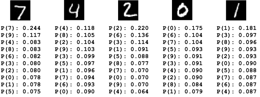
The accuracy of recognition of our quantum-mechanical network turns out to be somewhat worse than the classical, because in the process of modelling the Monte Carlo method is used, which adds a certain portion of randomness. Output of our network is shown in Fig. 23. As can be seen, the proposed scheme for obtaining $\varepsilon_{exc}$ from the classical weights is appeared to be satisfactory.

5 Conclusion

A neural network model based on the behavior of a interacting particles in a two-humped potential was proposed. Excitatory and inhibitory connections of neurons were introduced. It has been shown that it is possible to implement the simplest logical elements using such neurons and their connections. Simplest convolutional neural network recognizing vertical line has been constructed. We finally proposed the quantum neural network that performs digit recognition with satisfactory precession. In the case of simple architectures the possibility of transferring weights from classical neural network to a quantum one was demonstrated.

References

- [1] Yann LeCun, Bernhard Boser, John S Denker, Donnie Henderson, Richard E Howard, Wayne Hubbard, and Lawrence D Jackel. Backpropagation applied to handwritten zip code recognition. Neural computation, 1(4):541–551, 1989.
- [2] A. Graves, A. r. Mohamed, and G. Hinton. Speech recognition with deep recurrent neural networks. In 2013 IEEE International Conference on Acoustics, Speech and Signal Processing, pages 6645–6649, May 2013.
- [3] Yonghui Wu, Mike Schuster, Zhifeng Chen, Quoc V Le, Mohammad Norouzi, Wolfgang Macherey, Maxim Krikun, Yuan Cao, Qin Gao, Klaus Macherey, et al. Google’s neural machine translation system: Bridging the gap between human and machine translation. arXiv preprint arXiv:1609.08144, 2016.
- [4] Alexander M Polyakov. Gauge fields and strings. Contemp. Concepts Phys., 3:1–301, 1987.
- [5] D. M. Ceperley. Path integrals in the theory of condensed helium. Rev. Mod. Phys 67, 279, 1995.
- [6] Alex Krizhevsky, Ilya Sutskever, and Geoffrey E Hinton. Imagenet classification with deep convolutional neural networks. In F. Pereira, C. J. C. Burges, L. Bottou, and K. Q. Weinberger, editors, Advances in Neural Information Processing Systems 25, pages 1097–1105. Curran Associates, Inc., 2012.
- [7] Y. LeCun, L. Bottou, Y. Bengio, and P. Haffner. Gradient-based learning applied to document recognition. Proceedings of the IEEE, 86(11):2278–2324, November 1998.