Measurement quench in many-body systems

Abstract

Measurement is one of the key concepts which discriminates classical and quantum physics. Unlike classical systems, a measurement on a quantum system typically alters it drastically as a result of wave function collapse. Here we suggest that this feature can be exploited for inducing quench dynamics in a many-body system while leaving its Hamiltonian unchanged. Importantly, by doing away with dedicated macroscopic devices for inducing a quench – using instead the indispensable measurement apparatus only – the protocol is expected to be easier to implement and more resilient against decoherence. By way of various case studies, we show that our scheme also has decisive advantages beyond reducing decoherence – for spectroscopy purposes and probing nonequilibrium scaling of critical and quantum impurity many-body systems.

Introduction.– Measurement is a fundamental concept which discriminates between the classical and quantum worlds. While in the classical regime measurement is noninvasive with no effect on the system, in the quantum domain, however, acquiring information, even through a local measurement, comes at the cost of an abrupt wave-function collapse which affects the entire system. The fundamental tests for the validity of quantum mechanics, such as the violation of Bell Bell (1964); Aspect et al. (1981) and Legett-Garg Leggett and Garg (1985) inequalities are based on quantum measurements. Moreover, they are crucial ingredients of almost all emerging quantum technologies such as quantum teleportation Bennett et al. (1993), measurement-based quantum computation Briegel et al. (2009), fault-tolerant quantum computation Lo et al. (1998) and spin-chain quantum communication Shizume et al. (2007); Pouyandeh et al. (2014); Bayat and Omar (2015).

All quantum protocols consist of preparation, manipulation and readout of one or more particles. While preparation and manipulation can be achieved by different means, the readout is unequivocally accomplished by measurements. Experimentally, these all rely on macroscopic devices which may induce decoherence and increase the complexity of the process. This raises the question: Is it possible to simplify the whole process by keeping only the indispensable part of the macroscopic devices, i.e. the measurement apparatus, for the complete preparation and manipulation of the system?

To answer the question, one should first recall that a key task of any quantum protocol is to induce the “right” kind of dynamics on a system. A particularly important class is that of quench dynamics, where the time evolution is induced in the system by a sudden change in the Hamiltonian. Quantum quench physics has been the subject of extensive studies Polkovnikov et al. (2011); Eisert et al. (2015), addressing fundamental problems such as equilibration Rigol et al. (2008); Gogolin and Eisert (2016) and emergence of highly entangled states Barmettler et al. (2009) to practical applications such as creating long-distance entanglement Bayat et al. (2010a). Experimentally, various features of quench dynamics have been observed in optical lattices Cheneau et al. (2012); Zeiher et al. (2017); Fukuhara et al. (2013a, b), optical tweezers Bernien et al. (2017), ion-traps Jurcevic et al. (2014); Richerme et al. (2014), nuclear magnetic resonance devices Rao et al. (2014) and coupled optical fibers Bellec et al. (2012); Perez-Leija et al. (2013).

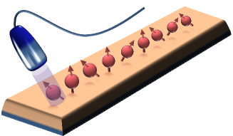
Figure 1: Measurement quench. A local measurement is performed on one of the qubits of a chain prepared in its ground state. This causes a collapse to a new state and induces dynamics in the system.

Here, we show that nonequilibrium dynamics can be induced by a local measurement, a measurement quench, keeping the Hamiltonian intact. We introduce several applications for this effect. Experimentally, a measurement quench uses the same measurement device that is used for reading the output signal, thus dispensing with the need for dedicated devices for inducing dynamics and therefore reduces decoherence. Note that, due to the wave function collapse, after a measurement quench the reduced density matrix of all subsystems change abruptly. This is very different from creating excitations via local rotations Jurcevic et al. (2014); Fukuhara et al. (2013a, b) in which only the local reduced density matrix of the rotated particles changes. Nonetheless, the same technology that performs local rotations can perform local measurements as well.

Measurement quench.– The notion of a measurement quench is most easily introduced by way of example. For this purpose, let us consider a chain of $N$ qubits interacting through a many-body Hamiltonian $H$. The system is initialized in its ground state $|E_{0}\rangle$. We then measure the magnetization of one of the qubits, say qubit $j$, in a certain basis which we here take as the Pauli $\sigma^{x}$ (cf. Fig. 1). The measurement is encoded by the two projectors

$$\Pi^{\uparrow}_{j}{=}|\uparrow_{j}\rangle\langle\uparrow_{j}|\otimes I_{rest},\quad\quad\Pi^{\downarrow}_{j}{=}|\downarrow_{j}\rangle\langle\downarrow_{j}|\otimes I_{rest},$$ (1)

where $\uparrow_{j}$ and $\downarrow_{j}$ represent the outcomes of the measurement in the $x$-direction at site $j$ and $I_{rest}$ denotes the identity operator in the space of all the other qubits. According to the outcome of the measurement, at time $t{=}0$, the wave function of the full system collapses to one of the following quantum states:

$$|\Psi^{\mu}_{j}(0)\rangle{=}\Pi^{\mu}_{j}|E_{0}\rangle/(p_{j}^{\mu})^{1/2},\quad p^{\mu}_{j}{=}\langle E_{0}|\Pi^{\mu}_{j}|E_{0}\rangle,\quad\mu{=}\uparrow,\downarrow.$$ (2)

Here $p^{\mu}_{j}$ is the probability of having the outcome $\mu_{j}$ for the measurement. Since the new quantum state is no longer an eigenstate of the Hamiltonian the system starts to evolve as

$$|\Psi^{\,\mu}_{j}(t)\rangle{=}e^{-iHt}|\Psi^{\,\mu}_{j}(0)\rangle=\sum_{n}e^{-iE_{n}t}|E_{n}\rangle\langle E_{n}|\Psi^{\,\mu}_{j}(0)\rangle,$$ (3)

where $E_{n}$ and $|E_{n}\rangle$ (for $n{=}0,1,\cdots$) are the eigenvalues and the eigenstates of $H$, respectively. Without loss of generality, from now on we assume that the outcome of the measurement is $\mu=\,\uparrow$ and drop the symbol $\mu$. The magnetization of the measured qubit $j$ at any later time $t$ is then given by $m_{j}^{x}(t){=}\langle\Psi^{\uparrow}_{j}(t)|\sigma^{x}_{j}|\Psi^{\uparrow}_{j}(t)\rangle$. It follows from Eq. (3) that

$$m_{j}^{x}(t)=\sum_{n,m}e^{-i(E_{n}-E_{m})t}\langle E_{m}|\sigma_{j}^{x}|E_{n}\rangle\langle E_{n}|\Psi_{j}^{\uparrow}(0)\rangle\langle\Psi_{j}^{\uparrow}(0)|E_{m}\rangle.$$ (4)

To read $m_{j}^{x}(t)$ one has to measure qubit $j$ again, which is the very same process that was used to induce the dynamics.

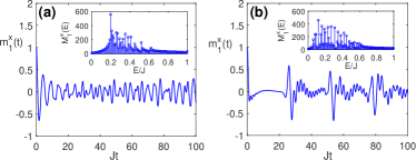
Figure 2: Transverse field Ising chain with long-range interaction. The magnetization $m_{1}^{x}(t)$ as a function of time in a chain of length $N=20$ and $B/J=1$ for two types of long-range interaction: (a) $\alpha=0.5$; (b) $\alpha=3$. The insets show the Fourier transform $M_{1}^{x}(E)$ as function of energy $E$ for the chosen value of $\alpha$.

Application 1: Spectroscopy.– Quantum simulation Lloyd et al. (1996); Cirac and Zoller (2012); Blatt and Roos (2012) is one of the most important goals of quantum technologies. Recently, simulating many-body systems with more than 50 particles have been possible with both cold atoms Bernien et al. (2017) and trapped ions Zhang et al. (2017). In fact, a wide range of spin Hamiltonians including the long-range Ising model Porras and Cirac (2004); Friedenauer et al. (2008) can be simulated in ion traps using either optical dipole forces Kielpinski et al. (2002) or inhomogeneous magnetic fields Mintert and Wunderlich (2001); Lekitsch et al. (2017); Zippilli et al. (2014). Local addressability is also available in these ion trap technologies NAÈgerl et al. (1999); Lekitsch et al. (2017). Spurred by these advances, the dynamics of the long-range transverse field Ising chain has attracted huge interest in both theory Schachenmayer et al. (2013) and experiment Zhang et al. (2017). The model is defined by Kim et al. (2009); Richerme et al. (2013)

$$H=J\sum_{i\neq j}\frac{1}{|i-j|^{\alpha}}\sigma_{i}^{x}\sigma_{j}^{x}+B\sum_{i}\sigma_{i}^{z},$$ (5)

where $\sigma_{i}^{x}$ and $\sigma_{i}^{z}$ are the Pauli matrices acting on site $i$, $B$ is a magnetic field strength, and $\alpha$ determines the range of the interaction such that $\alpha=0$ makes the system fully connected while the limit $\alpha\rightarrow\infty$ represents the nearest-neighbor chain. The exchange coupling is here taken to be antiferromagnetic, $J>0$. Current experimental techniques allow $\alpha$ to be tuned within the interval $0\leq\alpha\leq 3$ Monroe et al. (2015). Except for the special cases of $\alpha=0$ Lipkin et al. (1965); Russomanno et al. (2015) and $\alpha\rightarrow\infty$ Sachdev (2011), the Hamiltonian in (5) is not solvable and thus the spectrum can only be found for short chains through exact diagonalization. As shown in Ref. Schachenmayer et al. (2013), starting from a product state, the entanglement entropy grows linearly for short-range interactions (i.e. large $\alpha$) and logarithmically for long-range interactions (small $\alpha$) Schachenmayer et al. (2013).

As the Hamiltonian (5) commutes with the parity operator $P=\prod_{i=1}^{N}\sigma_{i}^{z}$, the ground state has always a definite parity. In particular, for even $N$, the ground state has even parity in which measuring $\sigma_{j}^{x}$ results in either $\uparrow_{j}$ or $\downarrow_{j}$ with equal probability. Eq. (4) can then be simplified to

$$m_{j}^{x}(t)=\sum_{n}\cos\left[\left(E_{n}-E_{0}\right)t\right]\left|\langle E_{n}|\sigma_{j}^{x}|E_{0}\rangle\right|^{2},$$ (6)

in which the frequencies of the oscillations are determined only by the energy gaps between the ground state $|E_{0}\rangle$ and those excited states $|E_{n}\rangle$ for which $|\langle E_{n}|\sigma_{j}^{x}|E_{0}\rangle|^{2}$ is nonzero. In Figs. 2(a)-(b) the local magnetization $m_{1}^{x}(t)$ is plotted versus time for $\alpha=0.5$ and $\alpha=3$ respectively in a system of length $N=20$, using open boundary conditions. As the figures show, for the larger $\alpha$ the dynamics equilibrates after a short oscillation and then revives due to the finite size of the system, while for the smaller $\alpha$ there is no hint of equilibration due to more frustration in the staggered ordering of the spins.

One may compute the Fourier transform of the local magnetization as $M_{j}^{x}(E)=\frac{1}{2\pi}\int_{0}^{\infty}m_{j}^{x}(t)e^{-iEt}dt$, which takes the form

$$M_{j}^{x}(E)=\sum_{n}\left|\langle E_{n}|\sigma_{j}^{x}|E_{0}\rangle\right|^{2}\bigl{[}\delta(E-E_{n}+E_{0})+\delta(E-E_{0}+E_{n})\bigr{]}/2.$$

In the insets of Figs. 2(a)-(b) we have plotted $M_{1}^{x}(E)$ for their respective dynamics. As is evident from the figures, more frequencies are excited for larger $\alpha$, resulting in the equilibration of $m_{1}^{x}(t)$ already on short time scales. The location of the peaks of $M_{1}^{x}(E)$ correspond to the energy gaps $E_{n}{-}E_{0}$ and thus $M_{1}^{x}(E)$ can be used as an efficient spectroscopic probe of an unsolvable system. In order to capture more eigenvalues of the Hamiltonian one can perform the measurement quench on other sites $j\!\neq\!1$ by which other eigenstates also get excited.

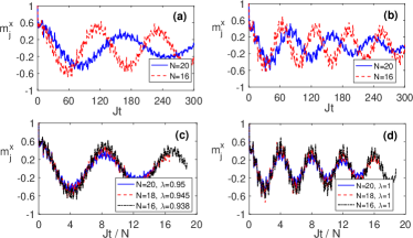
Figure 3: Magnetization dynamics in the transverse field Ising chain. Time evolution of the local magnetization after a measurement quench in the Ising model for: (a) $\lambda\!=\!0.95$; and (b) $\lambda\!=\!\lambda_{c}=\!1$. Nonequilibrium scaling of the local magnetization $m_{j}^{x}$ versus $t/N$ for (c) $|\lambda-\lambda_{c}|\simeq 1/N$ and (d) $|\lambda-\lambda_{c}|=0$, for which all lengths behave in the same way since $\xi\sim N$.

Application 2: Nonequilibrium scaling near a quantum phase transition.– Scaling is a key feature in many-body systems near criticality Sachdev (2011). Maybe the best known example from out-of-eqilibrium dynamics is the Kibble-Zurek scaling Kibble (1976); Zurek (1985); Kibble (2007), present when a many-body system is driven through a continuous phase transition at a finite rate. In a like manner, the asymptotic approach to equilibrium of a system that is suddenly quenched close to a quantum critical point is expected to be governed by equilibrium critical exponents De Grandi et al. (2010). Scaling in a critical system that has been subject to a global quench is expected only after long times Kennes et al. (2014). Local Hamiltonian quenches Eisler and Peschel (2007); Calabrese and Cardy (2007) also exhibit power-law scaling with time and distance from the quench Calabrese and Cardy (2007); Stéphan and Dubail (2011). Interestingly, the corresponding static scaling dimensions can be extracted at intermediate time scales Divakaran et al. (2011); Iglói et al. (2014). With this as a backdrop, one may inquire how a local measurement quench gives rise to scaling of observables.

To find out, let us consider the transverse-field Ising chain (TFIC). This model, solvable via Jordan-Wigner transformation, serves as a paradigm for quantum phase transitions Sachdev (2011). The Hamiltonian, masked as the limit $\alpha\!\rightarrow\!\infty$ in Eq. (5), is

$$H=\sum_{i=1}^{N}\sigma^{x}_{i}\sigma^{x}_{i+1}+\lambda\sum_{i=1}^{N}\sigma^{z}_{i}\,,$$ (7)

where the dimensionless parameter $\lambda$ plays the role of $B/J$ in the Hamiltonian (5), and here, in contrast to the previous example, periodic boundary conditions are imposed. By varying $\lambda$, the system undergoes a quantum phase transition at $\lambda\!=\!\lambda_{c}\!=\!1$, from an antiferromagnetic ($\lambda{<}\lambda_{c}$) to a paramagnetic ($\lambda{>}\lambda_{c}$) phase. Near the critical point the correlation length diverges as $\xi{\sim}|\lambda-\lambda_{c}|^{-\nu}$, with the exponent $\nu{=}1$ Sachdev (2011).

By translational invariance it does not matter on which site $j$ the measurement quench is performed. The well-defined parity of the TFIC eigenstates implies that $m_{j}^{x}(t)$ follows the Eq. (2). Unfortunately, the correlation functions $|\langle E_{n}|\sigma_{j}^{x}|E_{0}\rangle|^{2}$ in Eq. (2) cannot be expressed in terms of a finite number of free fermionic correlation functions in a periodic chain Barouch and McCoy (1971). This makes it difficult to benefit from a Jordan-Wigner transformation and instead we resort to numerical exact diagonalization. The result for $m_{j}^{x}(t)$ is plotted in Figs. 3(a) and (b) for $\lambda=0.95$ and $\lambda=\lambda_{c}=1$, respectively. The magnetization exhibits persistent small high-frequency fluctuations on top of a global oscillating low-frequency signal which decays slowly with time, suggesting gradual equilibration.

It is worth mentioning that the local magnetization $m_{j}^{x}$ is a non-equilibrium quantity and does not serve as an order parameter for the system. Therefore, it is not clear whether one can see scaling behavior for $m_{j}^{x}$. In fact, one may consider $m_{j}^{x}$ as a function of $t$, $N$ and $\xi$ where the dependence on $\lambda$ has been replaced by $\xi$ using $\xi\sim|\lambda-\lambda_{c}|^{-\nu}$. Scaling in the time evolution of $m_{j}^{x}$ means that it is not a function of $t,N$ and $\xi$ independently, but instead is parameterized as $m_{j}^{x}(t/N,N/\xi)$. To verify this, one fixes $N/\xi$ and then plots $m_{j}^{x}$ as a function of $t/N$ for various system sizes so that all curves collapse on top of each other. In order to fix $N/\xi$ one can choose $\lambda$ for each system size $N$ such that $N|\lambda-\lambda_{c}|^{\nu}$ remains fixed. In Fig. 3(c) such a data collapse is shown for three different system sizes. As the figure shows, that happens when $\nu$ is chosen to be $\nu=1$, i.e. the critical exponent known for the TFIC. An interesting case is $\lambda=\lambda_{c}$ for which all system sizes collapse on each other as in this case $N|\lambda-\lambda_{c}|^{\nu}$ becomes zero. As evident from Figs. 3(c) and (d), while the low-frequency signals show perfect data collapse, this is not so for the high-frequency fluctuations. This suggests that the two frequency components of $m_{j}^{x}$ have distinct characteristics: (i) the low-frequency part shows universal scaling behavior and thus exhibits perfect data collapse; and (ii) the small high-frequency part is non-universal and does not scale. Interestingly, the measurement quench is very different from the local Hamiltonian quenches at a defect in a critical TFIC in which the exponents are nonuniversal and vary with the defect parameter Iglói et al. (2014).

Application 3: Nonequilibrium scaling in the Kondo model.– The Kondo model Andrei et al. (1983); Hewson (1997); Pustilnik and Glazman (2004) serves as a paradigm for electronic many-body systems where the interaction with a quantum impurity dynamically generates a length scale. Taking advantage of the presence of this scale – the Kondo screening length $\xi_{K}$ – allows data from different systems to be collapsed onto a single curve, similar to a critical system like the TFIC discussed above. Theoretical work Ralph et al. (1994); Costi et al. (1994); Schiller and Hershfield (1995), as well as transport measurements on quantum dots in the Kondo regime Grobis et al. (2008), show that universal scaling behavior is maintained in nonequilibrium, and a Kondo cloud can form as the result of a local quench between an impurity and an electron gas Nuss et al. (2015). Moreover, a local Hamiltonian quench in a Kondo system may provide distance-independent entanglement between two distant impurities Bayat et al. (2010a). Here we add to the nonequilibrium picture of the Kondo physics, using a measurement quench.

For this purpose, it is more convenient to use a spin-chain emulation Laflorencie et al. (2008) of the Kondo model, allowing for efficient computations Bayat et al. (2010b) using the Density Matrix Renormalization Group (DMRG) White (1992, 1993). The spin chain has the Hamiltonian

$$H=J^{\prime}(J_{1}\boldsymbol{\sigma}_{1}\cdot\boldsymbol{\sigma}_{2}+J_{2}\boldsymbol{\sigma}_{1}\cdot\boldsymbol{\sigma}_{3})+J_{1}\sum_{i=2}^{N-1}\boldsymbol{\sigma}_{i}\cdot\boldsymbol{\sigma}_{i+1}+J_{2}\sum_{i=2}^{N-2}\boldsymbol{\sigma}_{i}\cdot\boldsymbol{\sigma}_{i+2}$$ (8)

where $J_{1}$ ($J_{2}$) is the (next-) nearest neighbor coupling and the dimensionless parameter $J^{\prime}$ represents the impurity coupling, with the impurity located at site $i=1$. By fine tuning $J_{2}/J_{1}=0.2412$ to the critical point of the spin-chain dimerization transition Laflorencie et al. (2008), the Hamiltonian in (8) provides a faithful representation of the spin sector of the Kondo model Laflorencie et al. (2008). The Kondo screening length $\xi_{K}$ can be identified with the spatial extent of a block of spins with which the impurity is maximally entangled Bayat et al. (2010b). Assuming that the number of sites on the chain is even, the SU(2) symmetry of the model implies that $p_{j}^{\uparrow}=1/2$. A measurement quench is now performed on the impurity spin at site $j=1$. To compute the subsequent time evolution, we employ exact diagonalization for short chains up to $N=20$ and time-dependent Runge-Kutta DMRG simulation for longer chains Feiguin and White (2005). Following the same finite-size scaling procedure as we used for the TFIC, we obtain the results displayed in Figs. 4(a)-(b), with $m_{1}^{x}(t)$ plotted versus $t/N$ when $N/\xi_{K}$ is fixed to $N/\xi_{K}=3.4$ and $N/\xi_{K}=2$, respectively. The value of $\xi_{K}$ is found using the entanglement approach of Ref. Bayat et al. (2010b).

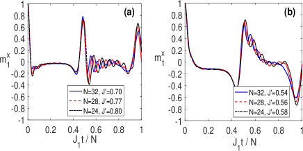
Figure 4: Magnetization dynamics in the Kondo model. Nonequilibrium scaling of the local magnetization $m_{1}^{x}$ versus $t/N$ when the length scale $\xi_{K}$ is tuned to: (a) $N/\xi_{K}\simeq 3.4$; (b) $N/\xi_{K}\simeq 2$.

As one can see, there are two distinct regions: (i) a scaling region which starts from $t=0$ and extends to $J_{1}t\backsimeq N/2$ over which there is an almost perfect data collapse; and (ii) a finite-size region $J_{1}t>N/2$ over which the data collapse gets distorted due to reflection of excitations from the boundaries. Note that the different scaling behaviors seen in the Kondo and TFIC models is due to the fact that the length scale $\xi_{K}$ is dynamically generated, and its divergence for small $J^{\prime}$ does not reflect a quantum phase transition.

It is worth pointing out that despite the success of DMRG to capture the low-energy sector of a many-body system, such as the Kondo model, it cannot compete with a real quantum simulator. First, as entanglement grows, the DMRG algortihm fails to give an accurate description Trotzky et al. (2012). Secondly, even for models where DMRG performs at its best the time scale to compute the evolution is order of magnitudes larger compared to monitoring the same dynamics on a real many-body system, like a quantum simulator using cold atom, trapped ions, or photonics. For such real-time experiments our measurement quench protocol is expected to come into its own.

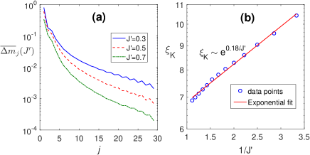
Figure 5: Detecting the Kondo cloud. (a) Average local magnetization difference $\overline{\Delta m}_{j}$ as function of measurement site $j$ in a chain of $N=32$ and $J^{\prime}=0.3$. (b) The length scale $\xi_{K}$ versus $1/J^{\prime}$ for the chain of length $N=32$ and $J^{\prime}=0.3$. The semilogarithmic plot confirms its exponential dependence with the fitting parameter $A=0.18$.

Application 4: Detecting the Kondo screening cloud.– While much is known about Kondo physics Andrei et al. (1983); Hewson (1997); Pustilnik and Glazman (2004), the experimental detection of the Kondo screening cloud, of size $\xi_{K}$, remains a challenge Affleck (2010). We here suggest a new type of protocol for determining $\xi_{K}$, based on a measurement quench. To do so, we consider the Hamiltonian in Eq. (8) and perform a measurement quench on the spin at site $j$. If this site is far from the impurity, outside the Kondo cloud, then the time evolution of the magnetization $m_{j}^{x}(t)$ is not affected by the presence of the impurity on short time scales. Thus, by comparing the evolution of $m_{j}^{x}(t)$ in the presence $(J^{\prime}\!\neq\!1)$ and absence $(J^{\prime}\!=\!1)$ of the impurity, one expects that there is no difference between the two cases when the site resides outside the Kondo cloud. Guided by this, we define an average local magnetization difference as

$$\overline{\Delta m}_{j}(J^{\prime})=\frac{1}{T}\int_{0}^{T}\left|m_{j}^{x}(J^{\prime})-m_{j}^{x}(J^{\prime}\!=\!1)\right|dt,$$ (9)

where $T=1/J^{\prime}$ is a short time compared to the time needed for spin excitations to propagate across the chain. In Fig. 5(a) we plot $\overline{\Delta m}_{j}(J^{\prime})$ as a function of $j$ for different values of $J^{\prime}$ in a spin chain of length $N=32$. As one can see from the figure, $\overline{\Delta m}_{j}(J^{\prime})$ decays exponentially when the site $j$ is far away from the impurity site $j\!=\!1$. By considering an exponential fitting function of the form $\overline{\Delta m}_{j}(J^{\prime}){\sim}e^{-j/\xi_{K}}$ to the tail of the data one can extract the length scale $\xi_{K}$. In Fig. 5(b) we plot $\xi_{K}$ thus obtained as a function of $1/J^{\prime}$. Choosing $A=0.18$, one obtains very good agreement with $\xi_{K}{\sim}e^{A/J^{\prime}}$, the expected exponential scaling for the Kondo screening length Hewson (1997).

Conclusion.– We have shown that a local measurement can be harnessed to induce nonequilibrium dynamics in many-body systems. In contrast to conventional quench protocols, where the Hamiltonian is manipulated, our proposal is easier to implement and less prone to decoherence. Several applications of measurement quenches have been discussed. They allow for efficient spectroscopy of nontrivial spin systems, for extracting nonequilibrium scaling at quantum criticality and in quantum impurity systems, and also for probing the elusive screening cloud in the Kondo model. Various physical setups, in which projective measurements have been realized, can potentially implement our protocol, including ion traps Mintert and Wunderlich (2001); Zhang et al. (2017); Lekitsch et al. (2017), optical lattices Sherson et al. (2010); Weitenberg et al. (2011); Fukuhara et al. (2013c, b), Rydberg atoms Bernien et al. (2017) and superconducting circuits Barends et al. (2016); Roushan et al. (2017). Importantly, a measurement quench can be performed on any initial state, including a thermal state and all the introduced applications remain valid if the temperature is small enough so that the measurement quench only excites low-energy eigenstates.

Acknowledgments.– AB thanks the University of Electronic Science and Technology of China for their support. SB and AB acknowledge the EPSRC grant $EP/K004077/1$ and the ERC under Starting Grant 308253 PACOMANEDIA. HJ acknowledges support from the Swedish Research Council through Grant No. 621-2014-5972.

References

- Bell (1964) J. S. Bell, Physics 1, 195 (1964).
- Aspect et al. (1981) A. Aspect, P. Grangier, and G. Roger, Phys. Rev. Lett. 47, 460 (1981).
- Leggett and Garg (1985) A. J. Leggett and A. Garg, Phys. Rev. Lett. 54, 857 (1985).
- Bennett et al. (1993) C. H. Bennett, G. Brassard, C. Crépeau, R. Jozsa, A. Peres, and W. K. Wootters, Phys. Rev. Lett. 70, 1895 (1993).
- Briegel et al. (2009) H. J. Briegel, D. E. Browne, W. Dür, R. Raussendorf, and M. Van den Nest, Nature Physics 5, 19 (2009).
- Lo et al. (1998) H.-K. Lo, T. Spiller, and S. Popescu, Introduction to quantum computation and information (World Scientific, 1998).
- Shizume et al. (2007) K. Shizume, K. Jacobs, D. Burgarth, and S. Bose, Phys. Rev. A 75, 062328 (2007).
- Pouyandeh et al. (2014) S. Pouyandeh, F. Shahbazi, and A. Bayat, Phys. Rev. A 90, 012337 (2014).
- Bayat and Omar (2015) A. Bayat and Y. Omar, New J. Phys. 17, 103041 (2015).
- Polkovnikov et al. (2011) A. Polkovnikov, K. Sengupta, A. Silva, and M. Vengalattore, Rev. Mod. Phys. 83, 863 (2011).
- Eisert et al. (2015) J. Eisert, M. Friesdorf, and C. Gogolin, Nature Physics 11, 124 (2015).
- Rigol et al. (2008) M. Rigol, V. Dunjko, and M. Olshanii, Nature 452, 854 (2008).
- Gogolin and Eisert (2016) C. Gogolin and J. Eisert, Rep. Prog. Phys. 79, 056001 (2016).
- Barmettler et al. (2009) P. Barmettler, M. Punk, V. Gritsev, E. Demler, and E. Altman, Phys. Rev. Lett. 102, 130603 (2009).
- Bayat et al. (2010a) A. Bayat, S. Bose, and P. Sodano, Phys. Rev. Lett. 105, 187204 (2010a).
- Cheneau et al. (2012) M. Cheneau, P. Barmettler, D. Poletti, M. Endres, P. Schauß, T. Fukuhara, C. Gross, I. Bloch, C. Kollath, and S. Kuhr, Nature 481, 484 (2012).
- Zeiher et al. (2017) J. Zeiher, J.-y. Choi, A. Rubio-Abadal, T. Pohl, R. van Bijnen, I. Bloch, and C. Gross, arXiv:1705.08372 (2017).
- Fukuhara et al. (2013a) T. Fukuhara, A. Kantian, M. Endres, M. Cheneau, P. Schauß, S. Hild, D. Bellem, U. Schollwöck, T. Giamarchi, C. Gross, et al., Nature Physics 9, 235 (2013a).
- Fukuhara et al. (2013b) T. Fukuhara, P. Schauß, M. Endres, S. Hild, M. Cheneau, I. Bloch, and C. Gross, Nature 502, 76 (2013b).
- Bernien et al. (2017) H. Bernien, S. Schwartz, A. Keesling, H. Levine, A. Omran, H. Pichler, S. Choi, A. S. Zibrov, M. Endres, M. Greiner, et al., Nature 551, 579 (2017).
- Jurcevic et al. (2014) P. Jurcevic, B. P. Lanyon, P. Hauke, C. Hempel, P. Zoller, R. Blatt, and C. F. Roos, Nature 511, 202 (2014).
- Richerme et al. (2014) P. Richerme, Z.-X. Gong, A. Lee, C. Senko, J. Smith, M. Foss-Feig, S. Michalakis, A. V. Gorshkov, and C. Monroe, Nature 511, 198 (2014).
- Rao et al. (2014) K. R. K. Rao, T. Mahesh, and A. Kumar, Physical Review A 90, 012306 (2014).
- Bellec et al. (2012) M. Bellec, G. M. Nikolopoulos, and S. Tzortzakis, Opt. Lett. 37, 4504 (2012).
- Perez-Leija et al. (2013) A. Perez-Leija, R. Keil, A. Kay, H. Moya-Cessa, S. Nolte, L.-C. Kwek, B. M. Rodríguez-Lara, A. Szameit, and D. N. Christodoulides, Phys. Rev. A 87, 012309 (2013).
- Lloyd et al. (1996) S. Lloyd et al., Science , 1073 (1996).
- Cirac and Zoller (2012) J. I. Cirac and P. Zoller, Nature Physics 8, 264 (2012).
- Blatt and Roos (2012) R. Blatt and C. F. Roos, Nature Phys. 8, 277 (2012).
- Zhang et al. (2017) J. Zhang, G. Pagano, P. W. Hess, A. Kyprianidis, P. Becker, H. Kaplan, A. V. Gorshkov, Z.-X. Gong, and C. Monroe, Nature 551, 601 (2017).
- Porras and Cirac (2004) D. Porras and J. I. Cirac, Phys.l Rev. Lett. 92, 207901 (2004).
- Friedenauer et al. (2008) A. Friedenauer, H. Schmitz, J. T. Glueckert, D. Porras, and T. Schätz, Nature Physics 4, 757 (2008).
- Kielpinski et al. (2002) D. Kielpinski, C. Monroe, and D. J. Wineland, Nature 417, 709 (2002).
- Mintert and Wunderlich (2001) F. Mintert and C. Wunderlich, Phys. Rev. Lett. 87, 257904 (2001).
- Lekitsch et al. (2017) B. Lekitsch, S. Weidt, A. G. Fowler, K. Mølmer, S. J. Devitt, C. Wunderlich, and W. K. Hensinger, Science Advances 3, e1601540 (2017).
- Zippilli et al. (2014) S. Zippilli, M. Johanning, S. Giampaolo, C. Wunderlich, and F. Illuminati, Phys. Rev. A 89, 042308 (2014).
- NAÈgerl et al. (1999) H. C. NAÈgerl, D. Leibfried, H. Rohde, G. Thalhammer, J. Eschner, F. Schmidt-Kaler, and R. Blatt, Phys. Rev. A 60, 145 (1999).
- Schachenmayer et al. (2013) J. Schachenmayer, B. Lanyon, C. Roos, and A. Daley, Phys. Rev. X 3, 031015 (2013).
- Kim et al. (2009) K. Kim, M.-S. Chang, R. Islam, S. Korenblit, L.-M. Duan, and C. Monroe, Phys. Rev. Lett. 103, 120502 (2009).
- Richerme et al. (2013) P. Richerme, C. Senko, S. Korenblit, J. Smith, A. Lee, R. Islam, W. C. Campbell, and C. Monroe, Phys. Rev. Lett. 111, 100506 (2013).
- Monroe et al. (2015) C. Monroe, W. Campbell, E. Edwards, R. Islam, D. Kafri, S. Korenblit, A. Lee, P. Richerme, C. Senko, and J. Smith, Proceedings of the International School of Physics ‘Enrico Fermi,’ Course 189 , 169 (2015).
- Lipkin et al. (1965) H. J. Lipkin, N. Meshkov, and A. Glick, Nucl. Phys. 62, 188 (1965).
- Russomanno et al. (2015) A. Russomanno, R. Fazio, and G. E. Santoro, EPL 110, 37005 (2015).
- Sachdev (2011) S. Sachdev, Quantum phase transitions (Cambridge university press, 2011).
- Kibble (1976) T. W. Kibble, J. of Phys. A: Math. Gen. 9, 1387 (1976).
- Zurek (1985) W. H. Zurek, Nature 317, 505 (1985).
- Kibble (2007) T. Kibble, Physics Today 60, 47 (2007).
- De Grandi et al. (2010) C. De Grandi, V. Gritsev, and A. Polkovnikov, Phys. Rev. B 81, 012303 (2010).
- Kennes et al. (2014) D. Kennes, V. Meden, and R. Vasseur, Phys. Rev. B 90, 115101 (2014).
- Eisler and Peschel (2007) V. Eisler and I. Peschel, J. Stat. Mech.: Theory and Experiment , P06005 (2007).
- Calabrese and Cardy (2007) P. Calabrese and J. Cardy, J. Stat. Mech.: Theory and Experiment , P10004 (2007).
- Stéphan and Dubail (2011) J.-M. Stéphan and J. Dubail, J. Stat. Mech.: Theory and Experiment 2011, P08019 (2011).
- Divakaran et al. (2011) U. Divakaran, F. Iglói, and H. Rieger, J. Stat. Mech.: Theory and Experiment , P10027 (2011).
- Iglói et al. (2014) F. Iglói, G. Roósz, and L. Turban, J. Stat. Mech.: Theory and Experiment , P03023 (2014).
- Barouch and McCoy (1971) E. Barouch and B. M. McCoy, Phys. Rev. A 3, 786 (1971).
- Andrei et al. (1983) N. Andrei, K. Furuya, and J. H. Lowenstein, Rev. Mod. Phys. 55, 331 (1983).
- Hewson (1997) A. C. Hewson, The Kondo problem to heavy fermions, Vol. 2 (Cambridge university press, 1997).
- Pustilnik and Glazman (2004) M. Pustilnik and L. Glazman, J. Phys. Condens. Matter 16, R513 (2004).
- Ralph et al. (1994) D. C. Ralph, A. W. W. Ludwig, J. von Delft, and R. A. Buhrman, Phys. Rev. Lett. 72, 1064 (1994).
- Costi et al. (1994) T. A. Costi, A. C. Hewson, and V. Zlatic, J. Phys. Condens. Matter 6, 2519 (1994).
- Schiller and Hershfield (1995) A. Schiller and S. Hershfield, Phys. Rev. B 51, 12896 (1995).
- Grobis et al. (2008) M. Grobis, I. G. Rau, R. M. Potok, H. Shtrikman, and D. Goldhaber-Gordon, Phys. Rev. Lett. 100, 246601 (2008).
- Nuss et al. (2015) M. Nuss, M. Ganahl, E. Arrigoni, W. von der Linden, and H. G. Evertz, Phys. Rev. B 91, 085127 (2015).
- Laflorencie et al. (2008) N. Laflorencie, E. S. Sørensen, and I. Affleck, J. Stat. Mech.: Theory and Experiment , P02007 (2008).
- Bayat et al. (2010b) A. Bayat, P. Sodano, and S. Bose, Phys. Rev. B 81, 064429 (2010b).
- White (1992) S. R. White, Phys. Rev. Lett. 69, 2863 (1992).
- White (1993) S. R. White, Phys. Rev. B 48, 10345 (1993).
- Feiguin and White (2005) A. E. Feiguin and S. R. White, Phys. Rev. B 72, 020404 (2005).
- Trotzky et al. (2012) S. Trotzky, Y.-A. Chen, A. Flesch, I. P. McCulloch, U. Schollwöck, J. Eisert, and I. Bloch, Nat. Phys. 8, 325 (2012).
- Affleck (2010) I. Affleck, “Perspectives on mesoscopic physics: Dedicated to professor yoseph imry’s 70th birthday,” (World Scientific, Singapore, 2010) pp. 1–44.
- Sherson et al. (2010) J. F. Sherson, C. Weitenberg, M. Endres, M. Cheneau, I. Bloch, and S. Kuhr, Nature 467, 68 (2010).
- Weitenberg et al. (2011) C. Weitenberg, M. Endres, J. F. Sherson, M. Cheneau, P. Schauß, T. Fukuhara, I. Bloch, and S. Kuhr, Nature 471, 319 (2011).
- Fukuhara et al. (2013c) T. Fukuhara, A. Kantian, M. Endres, M. Cheneau, P. Schauß, S. Hild, D. Bellem, U. Schollwöck, T. Giamarchi, C. Gross, et al., Nature Phys. 9, 235 (2013c).
- Barends et al. (2016) R. Barends, A. Shabani, L. Lamata, J. Kelly, A. Mezzacapo, U. Las Heras, R. Babbush, A. G. Fowler, B. Campbell, Y. Chen, et al., Nature 534, 222 (2016).
- Roushan et al. (2017) P. Roushan, C. Neill, J. Tangpanitanon, V. Bastidas, A. Megrant, R. Barends, Y. Chen, Z. Chen, B. Chiaro, A. Dunsworth, et al., Science 358, 1175 (2017).