Robustness of the deepest projection regression functional

Abstract

Depth notions in regression have been systematically proposed and examined in Zuo (2018). One of the prominent advantages of the notion of depth is that it can be directly utilized to introduce median-type deepest estimating functionals (or estimators in the case of empirical distributions) for location or regression parameters in a multi-dimensional setting.

Regression depth shares the advantage. Depth induced deepest estimating functionals are expected to inherit desirable and inherent robustness properties ( e.g. bounded maximum bias and influence function and high breakdown point) as their univariate location counterpart does. Investigating and verifying the robustness of the deepest projection estimating functional (in terms of maximum bias, asymptotic and finite sample breakdown point, and influence function) is the major goal of this article. It turns out that the deepest projection estimating functional possesses a bounded influence function and the best possible asymptotic breakdown point as well as the best finite sample breakdown point with robust choice of its univariate regression and scale component.
MSC 2010 Classification: Primary 62G05; Secondary 62G08, 62G35, 62G30.

Key words and phrase: Depth, linear regression, deepest regression estimating functionals, maximum bias, breakdown point, influence function, robustness.

Running title: Robustness of deepest regression functional.

1 Introduction

Consider a general linear regression model

$$y = \mathbf{x}^{\prime}\boldsymbol{\beta}+{{e}},$$ (1)

where $y$ and ${e}$ are univariate random variables, ^′ denotes the transpose of a vector, and random vector $\mathbf{x}=(x_{1},\cdots,x_{p})^{\prime}$ and unknown parameter $\boldsymbol{\beta}$ are in $\mathbb{R}^{p}$, the error ${e}$ has distribution $F_{{e}}$ and the random vector $\mathbf{x}$ has distribution $F_{\mathbf{x}}$. Note that this general model includes the special case with an intercept term. For example, if $\boldsymbol{\beta}=(\beta_{1},\boldsymbol{\beta_{2}}^{\prime})^{\prime}$ and $x_{1}=1$, then one has $y=\beta_{1}+\mathbf{x_{2}}^{\prime}\boldsymbol{\beta_{2}}+{e}$, where $\mathbf{x_{2}}=(x_{2},\cdots,x_{p})\in\mathbb{R}^{p-1}$. If one denotes $\mathbf{w}=(1,\mathbf{x_{2}}^{\prime})^{\prime}$, then $y=\mathbf{w}^{\prime}\boldsymbol{\beta}+{e}$. We use this model or (1) interchangably depending on the context. Denote by $F_{(y,~{}\mathbf{x})}$ the joint distribution of $y$ and $\mathbf{x}$ under the model (1). Let $T(\cdot)$ be a $\mathbb{R}^{p}$-valued estimating functional for $\boldsymbol{\beta}$, defined on the set ${\mathcal{G}}$ of distributions on $\mathbb{R}^{p+1}$. $T$ is called Fisher consistent for $\boldsymbol{\beta}$ if $T(F_{(y,~{}\mathbf{x})})=\boldsymbol{\beta}_{0}$ for the true parameter $\boldsymbol{\beta}_{0}\in\mathbb{R}^{p}$ of the model and for $F_{(y,~{}\mathbf{x})}\in{\mathcal{G}_{1}}\subset{\mathcal{G}}$, each member of ${\mathcal{G}_{1}}$ possesses some common attributes. Additional desirable properties of a regression functional $T(\cdot)$ are regression, scale, and affine equivariant. That is, $T(F_{(y+\mathbf{x}^{\prime}b,~{}\mathbf{x})})=T(F_{(y,~{}\mathbf{x})})+b,\forall~{}b\in\mathbb{R}^{p};$  $T(F_{(sy,~{}\mathbf{x})})=sT(F_{(y,~{}\mathbf{x})}),\forall~{}s\in\mathbb{R};$ $T(F_{(y,~{}A^{\prime}\mathbf{x})})=A^{-1}T(F_{(y,~{}\mathbf{x})}),\forall\mbox{~{}nonsingular $A\in\mathbb{R}^{p\times p}$}$; respectively. Namely, $T(\cdot)$ does not depend on the underlying coordinate system and measurement scale. The classical regression estimating functional is the least square (LS) functional. It meets all the desired properties above and is “optimal” if $F_{e}$ is normal (Huber (1972)). But it is extremely sensitive to a slight deviation from the normality assumption. Alternatives include the least absolute deviation functional, and quantile regression (Koenker and Bassett (1978)) were posed. But in terms of asymptotic breakdown point (ABP) robustness, they are no better than the traditional LS functional (all have $0\%$ ABP). Estimating functionals with higher ABP were consequently proposed. Among them, the least median squares estimator (Rousseeuw (1984)) is the most famous one. It has the highest ABP ($50\%$) but suffers a slow convergence rate (cubic root) (Davies (1989 and Kim and Pollard (1990)) and a instability drawback (Figure 3.2 of Seber and Lee (2003)). Robust estimating functionals with high ABP and root $n$ convergence rate were subsequently advanced. Among many of them is the regression depth (RD) induced deepest regression estimating functional (Rousseeuw and Hubert (1999) (RH99)) ($T^{*}_{RD}$). The latter has an ABP $1/3$ (Van Aelst and Rousseeuw (2000) (VAR00)) and root $n$ consistency (Bai and He (1999)). One of the prominent advantages of depth notion is that it can be directly employed to introduce median-type deepest estimating functionals (or estimators in the empirical case) for the location or regression parameter in a multi-dimensional setting based on a general min-max stratagem. The most outstanding feature of the univariate median is its exceptional robustness. Indeed, it has the best possible finite sample breakdown point (FSBP) (among all location equivariant estimators, see Donoho (1982)) and the minimum maximum bias (MB) (if the underlying distribution has a unimodal symmetric density, see Huber (1964)). The functional in RH99 ($T^{*}_{RD}$) holds desired properties, its ABP ($1/3$) is lower than the highest ($1/2$) though. The deepest projection estimating functional ($T^{*}_{PRD}$) induced from projection regression depth (PRD) in Zuo (2018)(Z18) overcomes this. It has the best ABP with a root n consistency ((Z18)) as well. $T^{*}_{PRD}$ is closely related to the bias-robust estimates (P-estimates) of Marrona and Yohai (1993) (MY93). In fact, it is a modified version of the latter, achieving the scale-invariance (see Section 2).

MY93 investigated the robustness of P-estimates, provided an upper bound of their MB, but their influence function (IF) and FSBP had not been explicitly established in the last quarter of century. Establishing a MB upper bound for $T^{*}_{PRD}$ and discovering its IF and revealing its exact FSBP are three main objectives of this article.

The rest of the article is organized as follows. Section 2 introduces the $T^{*}_{PRD}$. Section 3 is devoted to the establishment of MB, IF and FSBP of $T^{*}_{PRD}$. Section 4 addresses the computation issues of the deepest regression estimators, and presents data examples to illustrate the performance (in terms of robustness) of the regression lines of the LS, the $T^{*}_{RD}$ and the $T^{*}_{PRD}$, and carries out some simulations to investigate the finite-sample relative efficiency of $T^{*}_{RD}$ and the $T^{*}_{PRD}$. Brief concluding remarks end the article in Section 5.

2 Maximum projection regression depth functionals

Let us first recall the projection regression depth and its induced deepest estimating functionals defined in Z18. Assume that $T$ is a univariate regression estimating functional which satisfies
(A1) regression, scale and affine equivariant, that is,

$T(F_{(y+x{b},~{}{x})})=T(F_{(y,~{}{x})})+{b}$,  $\forall~{}{b}\in\mathbb{R}$, and

$T(F_{(sy,~{}{x})})=sT(F_{(y,~{}{x})})$,  $\forall~{}s\in\mathbb{R}$, and

$T(F_{(y,~{}a{x})})=a^{-1}T(F_{(y,~{}{x})})$,  $\forall~{}a(\neq 0)\in\mathbb{R}$.

respectively, where $x,y\in\mathbb{R}$ are random variables (r.v.s). Throughout the lower case $x$ is in $R$ while bold $\mathbf{x}$ is a vector.Let $S$ be a positive scale estimating functional such that

(A2) $S(F_{sz+b})=|s|S({F_{z}})$ for any r.v. $z\in\mathbb{R}$ and scalar $b,s\in\mathbb{R}$, that is, $S$ is scale equivariant and location invariant.

Equipped with a pair of $T$ and $S$, we can introduce a corresponding projection based multiple regression estimating functional. Define

$$\mbox{UF}_{\mathbf{v}}(\boldsymbol{\beta};~{}F_{(y,~{}\mathbf{x})},T):=|T(F_{(y-\mathbf{x}^{\prime}\boldsymbol{\beta},~{}\mathbf{x}^{\prime}\mathbf{v})})|/S(F_{y}),$$ (2)

which represents unfitness of $\boldsymbol{\beta}$ at $F_{(y,~{}\mathbf{x})}$ w.r.t. $T$ along the $\mathbf{v}\in\mathbb{S}^{p-1}:=\{u:\|u\|=1,u\in\mathbb{R}^{p}\}$. If $T$ is a Fisher consistent regression estimating functional, then $T(F_{(y-\mathbf{x}^{\prime}\boldsymbol{\beta}_{0},~{}\mathbf{x}^{\prime}\mathbf{v})})=0$ for some $\boldsymbol{\beta}_{0}$ (the true parameter of the model) and $\forall~{}\mathbf{v}\in\mathbb{S}^{p-1}$. Then, overall one expects $|T|$ to be small and close to zero for a candidate $\boldsymbol{\beta}$, independent of the choice of $\mathbf{v}$ and $\mathbf{x}^{\prime}\mathbf{v}$. The magnitude of $|T|$ measures the unfitness of $\boldsymbol{\beta}$ along the $\mathbf{v}$. Taking the supremum over all $\mathbf{v}\in\mathbb{S}^{p-1}$, yields

$$\mbox{UF}(\boldsymbol{\beta};~{}F_{(y,~{}\mathbf{x})},T)=\sup_{\|\mathbf{v}\|=1}\mbox{UF}_{\mathbf{v}}(\boldsymbol{\beta};~{}F_{(y,~{}\mathbf{x})},T),$$ (3)

the unfitness of $\boldsymbol{\beta}$ at $F_{(y,~{}\mathbf{x})}$ w.r.t. $T$. Now applying the min-max scheme, we obtain the projection regression estimating functional (also denoted by $T^{*}_{\text{PRD}}$) w.r.t. the pair $(T,S)$

$$T^{*}(F_{(y,~{}\mathbf{x})},T) = \arg\!\min_{\boldsymbol{\beta}\in\mathbb{R}^{p}}\mbox{UF}(\boldsymbol{\beta};~{}F_{(y,~{}\mathbf{x})},T)$$

$$= \arg\!\max_{\boldsymbol{\beta}\in\mathbb{R}^{p}}\text{PRD}\left(\boldsymbol{\beta};~{}F_{(y,~{}\mathbf{x})},T\right),$$

where, the projection regression depth (PRD) function is defined as

$$\text{PRD}\left(\boldsymbol{\beta};~{}F_{(y,~{}\mathbf{x})},T\right)=\left(1+\mbox{UF}\big{(}\boldsymbol{\beta};~{}F_{(y,~{}\mathbf{x})},T\big{)}\right)^{-1},$$ (5)

Remarks 2.1(I) $\mbox{UF}(\boldsymbol{\beta};~{}F_{(y,~{}\mathbf{x})},T)$ or $\mbox{UF}(\boldsymbol{\beta};~{}F_{(y,~{}\mathbf{x})})$ corresponds to outlyingness $O(x,F)$, and $T^{*}(F_{(y,~{}\mathbf{x})})$ corresponds to the projection median functional $PM(F)$ in location setting (see Zuo (2003)). Note that in (2), (3) and (2), we have suppressed the scale $S$ since it does not involve $\mathbf{v}$ and is nominal. Sometimes we also suppress $T$ for convenience.

A similar $T^{*}$ was first introduced and studied in MY93, where it was called P1-estimate (denote it by $T_{P1}$, see (6)). However, they are different. The definition of $T^{*}$ here is different from $T_{P1}$ of MY93, the latter multiplies by $S(F_{\mathbf{v}^{\prime}\mathbf{x}})$ instead of dividing by $S(F_{y})$ in $\mbox{UF}_{v}(\boldsymbol{\beta};~{}F_{(y,~{}\mathbf{x})},T)$ here. Furthermore, MY93 did not talk about the “unfitness” (or “depth”). Corresponding to (2) here, they instead defined the following

$$A(\boldsymbol{\beta},\mathbf{v})=|T(F_{(y-\boldsymbol{\beta}^{\prime}\mathbf{x},~{}\mathbf{v}^{\prime}\mathbf{x})})|S(F_{\mathbf{v}^{\prime}\mathbf{x}}),$$

where $\mathbf{v},\boldsymbol{\beta}\in\mathbb{R}^{p}$. Their P1-estimate is defined as

$$T_{P1}=\arg\min_{\boldsymbol{\beta}\in\mathbb{R}^{p}}\sup_{\|\mathbf{v}\|=1}A(\boldsymbol{\beta},\mathbf{v}).$$ (6)

(II) It is readily seen that $A(\boldsymbol{\beta},\mathbf{v})$ is not scale invariant whereas $\mbox{UF}_{\mathbf{v}}(\boldsymbol{\beta};~{}F_{(y,~{}\mathbf{x})},T)$ is. $T^{*}$ is regression, scale, and affine equivariant. (III) Examples of $T$ include mean, quantile, and median( Med), and location functionals in Wu and Zuo (2009) (WZ09). Examples of $S$ include standard deviation functional, the median absolute deviations functional (MAD), and scale functionals in WZ08. Hereafter we write $\text{Med}(Z)$ rather than $\text{Med}(F_{Z})$. For the special choice of $T$ and $S$ in (2) such as

$$T(F_{(y-\mathbf{x}^{\prime}\boldsymbol{\beta},~{}\mathbf{x^{\prime}}\mathbf{v})}) = \text{Med}_{\mathbf{x^{\prime}}\mathbf{v}\neq 0}\big{(}\frac{y-\mathbf{x}^{\prime}\boldsymbol{\beta}}{\mathbf{x^{\prime}}\mathbf{v}}\big{)},$$

$$S(F_{y}) = \text{MAD}(F_{y}),$$

we have

$$\text{UF}(\boldsymbol{\beta};F_{(y,~{}\mathbf{x})})=\sup_{\|\mathbf{v}\|=1}\Big{|}\text{Med}_{\mathbf{x^{\prime}}\mathbf{v}\neq 0}\big{(}\frac{y-\mathbf{x}^{\prime}\boldsymbol{\beta}}{\mathbf{x^{\prime}}\mathbf{v}}\big{)}\Big{|}\bigg{/}\text{MAD}(F_{y}),$$ (7)

and

$$\text{PRD}\left(\boldsymbol{\beta};~{}F_{(y,~{}\mathbf{x})}\right)=\inf_{\|\mathbf{v}\|=1,\mathbf{x^{\prime}}\mathbf{v}\neq 0}\frac{\text{MAD}(F_{y})}{\text{MAD}(F_{y})+\Big{|}\text{Med}\big{(}\frac{y-\mathbf{x}^{\prime}\boldsymbol{\beta}}{\mathbf{x^{\prime}}\mathbf{v}}\big{)}\Big{|}}.$$ (8)

A special case of PRD above (the empirical case) is closely related to the so-called “centrality” in Hubert, Rousseeuw, and Van Aelst (2001) (HRVA01). In the definition of the latter, nevertheless, all the term of “MAD$(\cdot)$” on the RHS of (8) is divided by $\text{Med}|\mathbf{x^{\prime}}\mathbf{v}|$. $\blacksquare$

3 Robustness of the deepest projection regression functional

One of the main purposes of seeking the maximum depth estimating functional in regression is for the robustness consideration, since the classical LS functional is notorious sensitive to the deviation from the model assumptions (normality assumption) and to the contamination. On the other hand, a maximum depth estimating functional could be regarded as a median-type functional in regression. The latter in location is well-known for its exceptional robustness. Do the maximum projection depth estimating functionals inherit the inherent robustness properties of the location counterpart (and w.r.t. what types of robustness measure)?

3.1 Maximum bias

For a given distribution $F\in\mathbb{R}^{d}$ (hereafter $F\in\mathbb{R}^{d}$ really means that $F$ is defined on $\mathbb{R}^{d}$) and an $\varepsilon>0$, the version of $F$ contaminated by an $\varepsilon$ amount of an arbitrary distribution $G\in\mathbb{R}^{d}$ is denoted by $F(\varepsilon,G)=(1-\varepsilon)F+\varepsilon G$ (an $\varepsilon$ amount deviation from the assumed $F$). Here it is assumed that $\varepsilon\leq 1/2$, otherwise $F(\varepsilon,G)=G((1-\varepsilon),F)$, and one can’t distinguish which one is contaminated by which one. The maximum bias of a given general functional L under an $\varepsilon$ amount of contamination at $F$ is defined as (see Hampel, Ronchetti, Rousseeuw and Stahel (1986) (HRRS86))

$$\mbox{MB}(\varepsilon;L,F) = \sup_{G\in\mathbb{R}^{d}}\|L(F(\varepsilon,G))-L(F)\|,$$

where $\mbox{MB}(\varepsilon;L,F)$ is the maximum deviation (bias) of $L$ under an $\varepsilon$ amount of contamination at $F$ and it mainly measures the global robustness of $L$. For a given $L$ at $F$, it is desirable that $\mbox{MB}(\varepsilon;L,F)$ is bounded for an $\varepsilon(\leq 1/2)$ as large as possible.

The minimum amount $\varepsilon^{*}$ of contamination at $F$ which leads to an unbounded $\mbox{MB}(\varepsilon;L,F)$ is called the asymptotic breakdown point (ABP) of $L$ at $F$, $\varepsilon^{*}(L,F)=\inf\{\varepsilon:\mbox{MB}(\varepsilon;L,F)=\infty\}$.

For a given $F=F_{(y,~{}\mathbf{x})}\in\mathbb{R}^{p+1}$, write $F_{(\mathbf{v},\boldsymbol{\beta})}:=F_{(y-\mathbf{x}^{\prime}\mathbf{\boldsymbol{\beta}},~{}\mathbf{x}^{\prime}\mathbf{v})}$ for $\mathbf{v}\in\mathbb{S}^{p-1}$ and a given $\boldsymbol{\beta}\in\mathbb{R}^{p}$. Let $F_{y}$ be the marginal distribution based on $y\in\mathbb{R}$. For the univariate regression (and scale) estimating functional $T$ (and $S$) in Section 2 and an $\varepsilon>0$, define

$$B_{T}(\varepsilon;T,F) = \inf_{\boldsymbol{\beta}\in\mathbb{R}^{p}}\sup_{G\in\mathbb{R}^{2},\|\mathbf{v}\|=1}|T(F_{(\mathbf{v},\boldsymbol{\beta})}(\varepsilon,G))|,$$

$$C(\varepsilon;T,F) = \sup_{G\in\mathbb{R}^{2},\|\mathbf{v}\|=1}|T(F_{(\mathbf{v},\mathbf{0})})(\varepsilon,G))|,$$

$$B_{S}(\varepsilon;S,F) = \sup_{G\in\mathbb{R}}|S(F_{y}(\varepsilon,G))|,~{}~{}~{}~{}~{}~{}b(\varepsilon;S,F)~{}=~{}\inf_{G\in\mathbb{R}}|S(F_{y}(\varepsilon,G))|.$$

Proposition 3.1 For a given pair $(T,S)$,  $F=F_{(y,~{}\mathbf{x})}$, and an $\varepsilon>0$, assume that $T(F_{(\mathbf{v},\boldsymbol{0})})=0$, $\forall~{}\mathbf{v}\in\mathbb{S}^{(p-1)}$, and $b(\varepsilon;S,F)>0$ and $B_{S}(\varepsilon;S,F)<\infty$. Then for $T^{*}(F_{(y,~{}\mathbf{x})},T)$ in (2)

$$\mbox{MB}(\varepsilon;T^{*},F)\leq~{}B_{T}(\varepsilon;T,F)+C(\varepsilon;T,F).$$

Proof: By regression equivariance of the $T^{*}$ (see (II) of Remarks 2.1), assume (w.l.o.g) that $T^{*}(F)=0$. Then

$$\mbox{MB}(\varepsilon;T^{*},F)=\sup_{G\in\mathbb{R}^{p+1}}\|T^{*}(F(\varepsilon,G)\|.$$

For the given $F$ and a given $G\in\mathbb{R}^{p+1}$, denote $\boldsymbol{\beta}^{*}(\varepsilon,G):=T^{*}(F(\varepsilon,G))$ and $F(\varepsilon,G)=F_{\mathbf{z}^{*}}$ and $\mathbf{z}^{*}=(y^{*},{\mathbf{x}^{*}}^{\prime})^{\prime}\in\mathbb{R}^{p+1}$. Then we need to show that

$$\sup_{G\in\mathbb{R}^{p+1}}\|\boldsymbol{\beta}^{*}(\varepsilon,G)\|\leq B_{T}(\varepsilon;T,F)+C(\varepsilon;T,F).$$

For the given $G\in\mathbb{R}^{p+1}$ and $F$, by (2), (3), and (2), we have

$$\boldsymbol{\beta}^{*}(\varepsilon,G) = \arg\!\min_{\boldsymbol{\beta}\in\mathbb{R}^{p}}\mbox{UF}(F(\varepsilon,G);\boldsymbol{\beta},T)$$

$$= \arg\!\min_{\boldsymbol{\beta}\in\mathbb{R}^{p}}\!\sup_{\|v\|=1}\mbox{UF}_{\mathbf{v}}(F(\varepsilon,G);\boldsymbol{\beta},T)$$

Assume that $\boldsymbol{\beta}^{*}(\varepsilon,G)\neq 0$. Write $\boldsymbol{\beta}^{*}$ for $\boldsymbol{\beta}^{*}(\varepsilon,G)$ and let $v^{*}=\boldsymbol{\beta}^{*}/\|\boldsymbol{\beta}^{*}\|$, then we have by (A1) given in Section 2

$$|T(F_{(y^{*}-(\mathbf{x}^{*})^{\prime}\boldsymbol{\beta^{*}},~{}(\mathbf{x}^{*})^{\prime}\mathbf{v^{*}})})|=|T(F_{(y^{*},~{}(\mathbf{x}^{*})^{\prime}\mathbf{v^{*}})})-\|\boldsymbol{\beta}^{*}\||.$$

If $\|\boldsymbol{\beta}^{*}\|\leq\sup_{\|\mathbf{v}\|=1}|T(F_{(y^{*},~{}(\mathbf{x}^{*})^{\prime}\mathbf{v})}|$ for every given $G\in R^{p+1}$, then $\|\boldsymbol{\beta}^{*}\|\leq C(\varepsilon;T,F)$, we already have the desired result. Otherwise, we have for any given $\boldsymbol{\beta}\in\mathbb{R}^{p}$

$$\sup_{\|\mathbf{v}\|=1}|T(F_{(y^{*}-(\mathbf{x}^{*})^{\prime}\boldsymbol{\beta},~{}(\mathbf{x}^{*})^{\prime}\mathbf{v})})| \geq |T(F_{(y^{*}-(\mathbf{x}^{*})^{\prime}\boldsymbol{\beta^{*}},~{}(\mathbf{x}^{*})^{\prime}\mathbf{v^{*}})})|$$

$$\geq \|\boldsymbol{\beta}^{*}\|-|T(F_{(y^{*},~{}(\mathbf{x}^{*})^{\prime}\mathbf{v^{*}})}|$$

$$\geq \|\boldsymbol{\beta}^{*}\|-\sup_{\|\mathbf{v}\|=1}|T(F_{(y^{*},~{}(\mathbf{x}^{*})^{\prime}\mathbf{v})}|,$$

Therefore, we have for the given $G\in\mathbb{R}^{p+1}$ and $F$ and $\varepsilon$ and the given $\boldsymbol{\beta}\in\mathbb{R}^{p}$

$$\|\boldsymbol{\beta}^{*}(\varepsilon,G)\| \leq \sup_{\|\mathbf{v}\|=1}|T(F_{(y^{*}-(\mathbf{x}^{*})^{\prime}\boldsymbol{\beta},~{}(\mathbf{x}^{*})^{\prime}\mathbf{v})})|+\sup_{\|\mathbf{v}\|=1}|T(F_{(y^{*},~{}(\mathbf{x}^{*})^{\prime}\mathbf{v})})|$$

$$\leq \sup_{G\in\mathbb{R}^{2},\|\mathbf{v}\|=1}|T(F_{(\mathbf{v},\boldsymbol{\beta})}(\varepsilon,G))|+\sup_{G\in\mathbb{R}^{2},\|\mathbf{v}\|=1}|T(F_{(\mathbf{v},\boldsymbol{0})}(\varepsilon,G))|.$$

Taking the infimum over $\boldsymbol{\beta}\in\mathbb{R}^{p}$ and then supremum over $G\in\mathbb{R}^{(p+1)}$ in both sides immediately yields the desired result. This completes the proof. $\blacksquare$

Remarks 3.1(I) The assumption (A0): $T(F_{(\mathbf{v},0)})=T(F_{(y,~{}\mathbf{x}^{\prime}\mathbf{v})})=0$ for $\mathbf{v}\in\mathbb{S}^{p-1}$ is equivalent to the Fisher-consistency of $T$ or $F_{(y,~{}\mathbf{x})}$ is T-symmetric about $\mathbf{0}\in\mathbb{R}^{p}$. $F_{(y,~{}\mathbf{x})}$ is T-symmetric about a $\boldsymbol{\beta}_{0}$ iff

$$\textbf{(C0)}:~{}~{}~{}T\big{(}F_{(y-\mathbf{x^{\prime}}\boldsymbol{\beta}_{0},~{}\mathbf{x}^{\prime}\mathbf{v})}\big{)}=0,~{}\forall~{}\mathbf{v}\in\mathbb{S}^{p-1},$$ (9)

and it holds for a wide range of distributions $F_{(y,~{}\mathbf{x})}$ and $T$. For example, if the univariate functional $T$ is the mean functional, then this becomes the classical assumption in regression when $\boldsymbol{\beta}_{0}$ is the true parameter of the model: the conditional expectation of the error term ${e}$ (which is assumed to be independent of $\mathbf{x}$) given $\mathbf{x}$ is zero, i.e.

$$\textbf{(C1)}:~{}~{}~{}~{}E(F_{y-\mathbf{x^{\prime}}\boldsymbol{\beta_{0}}}\big{|}_{\mathbf{x}=\mathbf{x_{0}}})=E(F_{(y-\mathbf{x^{\prime}}\boldsymbol{\beta_{0}},\mathbf{x^{\prime}}\mathbf{v}})=0,~{}\forall~{}\mathbf{x_{0}}\in\mathbb{R}^{p-1},\mathbf{v}\in\mathbb{S}^{p-1}.\hskip 22.76219pt$$

(A0), however, is not indispensable in the proof but for the neatness of the upper bound and of the expression for $B_{T}(\varepsilon;T,F)$. Adding $\sup_{\|\mathbf{v}\|=1}|T(F_{(y,\mathbf{x}^{\prime}\mathbf{v})})|$ to the RHS of the upper bound and using the regular deviation definition for $B_{T}(\varepsilon;T,F)$, the proposition holds without (A0). (II) An upper bound for their P-estimates was also given in MY93 (Theorem 3.3). The two upper bounds are quite different due to the definition of $T^{*}$ is different from P-estimates.

(III) The conditions on $S$ in the proposition are typically satisfied by common scale functionals such as MAD or scale functionals in WZ08. The term $C(\varepsilon;T,F)$ in the Proposition is typically bounded for $T$ (such as quantile functionals or functionals in WZ09). (IV) The maximum projection regression depth functional $T^{*}$ has a bounded maximum bias as long as that is true for the $T$, and $S$ does not breakdown (for a scale functional, its ABP is defined as $\varepsilon^{*}(S,F)=\min\{\varepsilon:B_{S}(\varepsilon;S,F)+b(\varepsilon;S,F)^{-1}=\infty\}$). Furthermore, the MB upper bound of $T^{*}$ depends entirely on that of the $T$ as long as $S$ does not breakdown. The Proposition also reveals the ABP of $T^{*}$ as summarized in the following.   $\blacksquare$Corollary 3.1 Under the same assumptions of Proposition 3.1, we have

• (i) $\varepsilon^{*}(T^{*},F)\geq\min\big{\{}\varepsilon^{*}(T,F);\varepsilon^{*}(S,F)\big{\}}$.

• if $(T,S)=(\text{Med},~{}\text{MAD})$ then

• (ii) $\varepsilon^{*}(T^{*},F)=1/2$

Proof: (i) is trivial.

(ii) follows from the standard ABP results of Med and MAD (see e.g. HRRS86) and the upper bound of ABP for any regression equivariant functional (see Theorem 3.1 of Davies (1993) and of Davies and Gather (2005)). $\blacksquare$

Remarks 3.2(I) If the choice for $T$ and $S$ is $(\text{Med},~{}\text{MAD})$, then $T^{*}$ can have an ABP as high as $1/2$. HRVA01 reported their most central regression estimator $T^{c}_{r}$ (in Theorem 8) has a $50\%$ breakdown point without any rigorous treatment. $T^{c}_{r}$, however, is slightly different from $T^{*}(F_{n})$ here, see Remarks 2.1.

(II) The ABP of the deepest regression functional of RH 99 has been inventively studied in VAR00 and is $1/3$, while the ABP of the classical LS functional is $0$. $\blacksquare$When $(T,S)$ is $(\text{Med},~{}\text{MAD})$ , then the general bounds involved in Proposition 3.1 could be concretized and specified as shown in the following. Furthermore, one also could construct a lower bound for the maximum bias of $T^{*}$ in (2). First we need some notations. Write $q(\varepsilon)=1/(2(1-\varepsilon))$ for a given $0<\varepsilon<1/2$. Denote $m_{i}(Z,c,\varepsilon)$ for quantiles such that $m_{1}(Z,c,\varepsilon)=F_{|Z-c|}^{-1}(1-q(\varepsilon))$, $m_{2}(Z,c,\varepsilon)=F_{|Z-c|}^{-1}(q(\varepsilon))$ for a random variable $Z\in\mathbb{R}$ any scalar $c\in\mathbb{R}$ . Proposition 3.2 Let $T(F_{(y-\boldsymbol{x^{\prime}}\boldsymbol{\beta},~{}\mathbf{x}^{\prime}\mathbf{v})})=\text{Med}\big{(}\frac{y-\boldsymbol{x^{\prime}}\boldsymbol{\beta}}{\mathbf{x}^{\prime}\mathbf{v}}\big{)}$ ($\mathbf{x}^{\prime}\mathbf{v}\neq 0$ a.s.),  $S(F_{y})=\text{MAD}(F_{y})$. Assume that $1^{o}$) $F_{(y,\boldsymbol{x})}$ is $T$-symmetric about a $\boldsymbol{\beta_{0}}$ which is the true parameter of model (1); $2^{o}$) $F_{{e}}$ has a symmetric, decreasing in $|x|$ density $f(x)$; $3^{o}$) $F_{\mathbf{x}^{\prime}\mathbf{v}}$ is the same $\forall~{}\mathbf{v}\in\mathbb{S}^{p-1}$; $4^{o}$) $e$ and $\mathbf{x}$ are independent. Then, for the $T^{*}$ in (2), the given $F=F_{(y,~{}\mathbf{x})}$, any $0<\varepsilon<1/2$,

• (i) $T^{*}$ is Fisher-consistent. That is, $T^{*}(F,T)=\boldsymbol{\beta}_{0}$, under $1^{o})$;

• (ii) $B_{S}(\varepsilon;S,F)=c$, $b(\varepsilon;S,F)=d$, under $1^{o})$–$2^{o})$; $B_{T}(\varepsilon;T,F)=b$, under $3^{o}$);

• (iii) $\displaystyle b\leq\mbox{MB}(\varepsilon;T^{*},F)\leq b+C(\varepsilon;T,F)=2b$, under $1^{o})$–$4^{o})$;

where $b=J^{-1}\big{(}q(\varepsilon)\big{)}$, $c=m_{2}(y,a1,\varepsilon)$, $d=m_{1}(y,b1,\varepsilon)$, $a1=F_{|y|}^{-1}(1-q(\varepsilon))$, $b1=F_{|y|}^{-1}(q(\varepsilon))$. All quantiles is assumed to exist uniquely, $J$ is the distribution of $y/\mathbf{x}^{\prime}\mathbf{v}$,$\mathbf{v}\in\mathbb{S}^{p-1}$. To prove the statements above, we need the following result given in Zuo, Cui, and Young (2004) (ZCY04). Lemma 3.1  Suppose that $A=F^{-1}(1-q(\varepsilon))$ and $B=F^{-1}(q(\varepsilon))$ exist uniquely for $X\in\mathbb{R}$ with $F:=F_{X}$ and $0<\varepsilon<1/2$. Let $\delta_{x}$ denote the point-mass probability measure at $x\in\mathbb{R}$. Then for any distribution $G\in\mathbb{R}$ and point $x$,

• (L-i) $A\leq{\text{Med}}(F(\varepsilon,G))\leq B$,    (L-ii) ${\text{Med}}(F(\varepsilon,\delta_{x}))={\text{Med}}\{A,B,x\}$,

• (L-iii) $m1\big{(}X,{\text{Med}}(F(\varepsilon,G)),\varepsilon\big{)}\leq{\text{MAD}}(F(\varepsilon,G))\leq m2\big{(}X,{\text{Med}}(F(\varepsilon,G)),\varepsilon\big{)}$,

• (L-iv) ${\text{MAD}}(F(\varepsilon,\delta_{x}))={\text{Med}}\bigg{\{}m1\big{(}X,\text{Med}(F(\varepsilon,\delta_{x})),\varepsilon\big{)},~{}|x-{\text{Med}}(F(\varepsilon,\delta_{x}))|,\\ \hskip 136.57323pt~{}m2\big{(}X,{\text{Med}}(F(\varepsilon,\delta_{x})),\varepsilon\big{)}\bigg{\}}$.

where Med is applied to distributions as well as discrete points. $\blacksquare$

Proof of Proposition 3.2 (i) The given condition (assumption) guarantees that $T$ is Fisher-consistent at $F_{(y,\mathbf{x})}$, that is, for any $\mathbf{v}\in\mathbb{S}^{p-1}$

$$T\big{(}F_{(y-\mathbf{x}^{\prime}\boldsymbol{\beta_{0}},~{}\mathbf{x}^{\prime}\mathbf{v})}\big{)}=0.$$

Both (2) and (3) are equal to zero. That is, $\text{UF}(\boldsymbol{\beta}_{0};F_{(y,\mathbf{x})},T)=0.$ Therefore, $\boldsymbol{\beta}_{0}$ attains the minimum possible value of $\text{UF}(\boldsymbol{\beta};F_{(y,\mathbf{x})},T)$ for any $\boldsymbol{\beta}\in\mathbb{R}^{p}$, which further means that $T^{*}(F_{(y,~{}\mathbf{x})},T)=\boldsymbol{\beta}_{0}$. By the equivalence of $T^{*}$ (see Remarks 2.1), assume w.l.o.g. that $\boldsymbol{\beta}_{0}=\mathbf{0}$.

(ii) We need the maximum bias bounds on Med and MAD. Some of them have been already established in Lemma A.2 of ZCY04 (cited above in Lemma 3.1).

Note that when $\boldsymbol{\beta_{0}}=0$, $y$ has the same distribution as ${e}$, $m_{i}(y,c,\varepsilon)$ is nonincreasing in $c$ for $c>0$, the bounds for $S$ follow directly from this fact, coupled with (L-iii) and (L-i). We have to establish the bound for $T$. Note that

$$B_{T}(\varepsilon;T,F)=\inf_{\boldsymbol{\beta}\in\mathbb{R}^{p}}\sup_{G\in R^{2},\|\mathbf{v}\|=1}|T(F_{(\mathbf{v},\boldsymbol{\beta})}(\varepsilon;G))|.$$ (10)

To invoke (L-i) of the Lemma 3.1, we need to first determine the $B$ in (L-i) for the distribution of $Z:=(y-\mathbf{x}^{\prime}\boldsymbol{\beta})/(\mathbf{x}^{\prime}\mathbf{v})$ for a given $\boldsymbol{\beta}\in\mathbb{R}^{p}$ and a $\mathbf{v}\in\mathbb{S}^{p-1}$. Note that

$$Z=\frac{y-\mathbf{x}^{\prime}\boldsymbol{\beta}}{\mathbf{x}^{\prime}\mathbf{v}} = \frac{y-\mathbf{x}^{\prime}(\boldsymbol{\beta}-(\boldsymbol{\beta}^{\prime}\mathbf{v})\mathbf{v})-\mathbf{x}^{\prime}\mathbf{v}(\boldsymbol{\beta}^{\prime}\mathbf{v})}{\mathbf{x}^{\prime}\mathbf{v}}$$

$$:= \frac{y-\mathbf{x}^{\prime}\boldsymbol{\alpha}_{(\boldsymbol{\beta},\mathbf{v})}}{\mathbf{x}^{\prime}\mathbf{v}}-\boldsymbol{\beta}^{\prime}\mathbf{v}$$

$$:= Z1-\boldsymbol{\beta}^{\prime}\mathbf{v}.$$

For convenience we suppress the dependency of $Z$ and $Z1$ on $\boldsymbol{\beta}$ and $\mathbf{v}$. Note that $\|\boldsymbol{\alpha}_{(\boldsymbol{\beta},\mathbf{v})}\|=\|\boldsymbol{\beta}-(\boldsymbol{\beta}^{\prime}\mathbf{v})\mathbf{v}\|=(\|\boldsymbol{\beta}\|^{2}-(\boldsymbol{\beta}^{\prime}\mathbf{v})^{2})^{1/2}$ and $\boldsymbol{\alpha}^{\prime}_{(\boldsymbol{\beta},\mathbf{v})}\mathbf{v}=0$. It is readily seen that $F_{Z}(z)=F_{Z1}(z+\boldsymbol{\beta}^{\prime}\mathbf{v})$ and hence that $F_{Z}^{-1}(p)=F_{Z1}^{-1}(p)-\boldsymbol{\beta}^{\prime}\mathbf{v}$ for any $p\in(0,1)$. Now denote the distribution of $(y-\mathbf{x}^{\prime}\boldsymbol{\alpha})/\mathbf{x}^{\prime}\mathbf{v}$ with $\|\boldsymbol{\alpha}\|=r$ and $\boldsymbol{\alpha}^{\prime}\mathbf{v}=0$ by $J_{r}$ for any $\mathbf{v}\in\mathbb{S}^{p-1}$. Hence $F_{Z1}=J_{r}$ with $r=(\|\boldsymbol{\beta}\|^{2}-(\boldsymbol{\beta}^{\prime}\mathbf{v})^{2})^{1/2}$ for any $\mathbf{v}\in\mathbb{S}^{p-1}$ and a given $\boldsymbol{\beta}\in\mathbb{R}^{p}$. In the light of Lemma 3.1,

$$B_{T}(\varepsilon;T,F)=\inf_{\boldsymbol{\beta}\in\mathbb{R}^{p}}\sup_{\|v\|=1}\left|F^{-1}_{Z1}(q(\varepsilon))-\boldsymbol{\beta}^{\prime}\mathbf{v}\right|.$$ (11)

On the other hand,

$$\inf_{\boldsymbol{\beta}\in\mathbb{R}^{p}}\sup_{\|v\|=1}\left|F^{-1}_{Z1}(q(\varepsilon))-\boldsymbol{\beta}^{\prime}\mathbf{v}\right| \geq \inf_{\boldsymbol{\beta}\in\mathbb{R}^{p}}\left|J^{-1}_{0}(q(\varepsilon))-\|\boldsymbol{\beta}\|\right|$$

$$= \inf_{\boldsymbol{\beta}\in\mathbb{R}^{p}}\left|\|\boldsymbol{\beta}\|-J^{-1}_{0}(q(\varepsilon))\right|=J^{-1}_{0}(q(\varepsilon)),$$

where the first inequality follows from the consideration of a special $\mathbf{v}=\boldsymbol{\beta}/\|\boldsymbol{\beta}\|$ for $\boldsymbol{\beta}\neq 0$ and $3^{o}$), the second equality is due to the fact that $J^{-1}_{0}(q(\varepsilon))$ has nothing to do with $\boldsymbol{\beta}$. Therefore, by picking $\boldsymbol{\beta}=\mathbf{0}$ on the RHS of (11), its LHS attains its lower bound. That is, $B_{T}(\varepsilon;T,F)=J_{0}^{-1}(q(\varepsilon))$ which is the same as $b$ since when $r=0$, $J_{r}$ is the same as $J$ distributionally.

(iii) In virtue of (ii) above, one part of the RHS inequality has already been established in Proposition 3.1. But we still need to show that $C(\varepsilon;T,F)=b$. This, however, follows in a straightforward manner from the definition of $C(\varepsilon;T,F)$ and the proof in (ii) above (with $\boldsymbol{\beta}=\mathbf{0}$ in this case). We need to show the LHS lower bound for $\mbox{MB}(\varepsilon;T^{*},F)$. We adapt the idea of Huber (1981) (page 74-75). Note that for a given $\mathbf{v}\in\mathbb{S}^{p-1}$ by $4^{o}$)

$$F_{\mathbf{v}}(y,{z}):=F_{(y,~{}\mathbf{x}^{\prime}\mathbf{v})}(y,{z})=F_{(y-\boldsymbol{x}^{\prime}\boldsymbol{\beta}_{0},~{}\mathbf{x}^{\prime}\mathbf{v})}(y,{z})=F_{{e}}(y)F_{\mathbf{x}^{\prime}\mathbf{v}}({z}),~{}\text{for~{}}y,~{}z\in\mathbb{R}.$$

Assume that $\boldsymbol{x}\neq\boldsymbol{0}$, otherwise, our discussion reduces to Huber (1981) (page 74-75), our conclusion holds true. Assume, w.l.o.g., that the first component of $\boldsymbol{x}$, $x_{1}\neq 0$. Construct two functions:

$$F^{+}_{\mathbf{v}}(y,{z})=(1-\varepsilon)\big{[}F_{{e}}(y)\mathbf{I}_{y\leq ax_{1}}+F_{{e}}(y-2ax_{1})\mathbf{I}_{y>ax_{1}}\big{]}F_{\mathbf{x}^{\prime}\mathbf{v}}({z}),$$

$$F^{-}_{\mathbf{v}}(y,{z})=F^{+}_{(y,\mathbf{x})}(y+2ax_{1},{z}),$$

where $a=J^{-1}(q(\varepsilon))$ is the $q(\varepsilon)$th quantile of $y/\boldsymbol{x^{\prime}}\boldsymbol{v_{0}}(=y/x_{1})$ with $\boldsymbol{v_{0}}=(1,0,\cdots,0)^{\prime}\in\mathbb{R}^{p}$. It is now not difficult to verify that the two functions above are distribution functions over $\mathbb{R}^{2}$ and belong to $F_{\mathbf{v}}(\varepsilon;G)$ for some $G\in\mathbb{R}^{2}$(because both keep $(1-\varepsilon)$ part of $F_{\mathbf{v}}(y,{z})$).Assume that for some the random vector $(y^{*},\mathbf{x})$, $F_{(y^{*},~{}\mathbf{x}^{\prime}\mathbf{v})}=F_{\mathbf{v}}^{+}$. (note that vector $\mathbf{x}$ is unchanged due to the construction). Then one has $F_{\mathbf{v}}^{-}=F_{(y^{*}+2ax_{1},~{}\mathbf{x}^{\prime}\mathbf{v})}=F_{(y^{*}+\mathbf{x}^{\prime}\boldsymbol{\eta},~{}\mathbf{x}^{\prime}\mathbf{v})}$ with $\boldsymbol{\eta}=(2a,0,\cdots,0)^{\prime}\in\mathbb{R}^{p}$ Denote the first coordinate of $T^{*}(F)$ as $T^{*}_{1}(F)$. Then by the equivariance of $T^{*}$, we see that $T_{1}^{*}(F_{\mathbf{v_{0}}}^{+})-T^{*}_{1}(F_{\mathbf{v_{0}}}^{-})=-2a,$ which implies

$$2a \leq \sup_{\|\mathbf{v}\|=1}|T_{1}^{*}(F_{\mathbf{v}}^{+})-T_{1}^{*}(F_{\mathbf{v}}^{-})|$$

$$\leq 2\sup_{G\in\mathbb{R}^{2},\|\mathbf{v}\|=1}\|T^{*}(F_{\mathbf{v}}(\varepsilon;G))\|.$$

Note that $a=b$. This completes the entire proof. $\blacksquare$

Remarks 3.3

(I) Part (i) of the Proposition holds as long as $T$ is $T$-symmetric about a $\boldsymbol{\beta}_{0}\in\mathbb{R}^{p}$. That is, $T$ is not necessarily to be the Med functional. Furthermore, $S$ plays no role in the verification process, that is, any scale estimating functional will work. Likewise, the lower bound in (iii) holds true for any $T$ and $S$. The (Med, MAD) choice is just the classical one.

(II) The assumption that $F_{{e}}$ has a symmetric density $f(x)$ which is decreasing in $|x|$ is common and typically required in the literature (see, e.g., MY93, Theorem 3.5). It guarantees that the construction of the two functions are indeed distribution functions in the proof of (iii) (actually it guarantees that the probability mass covered by both $F_{{e}}(y)\mathbf{I}_{y\leq ax_{1}}$ and $F_{{e}}(y-2ax_{1})\mathbf{I}_{y>ax_{1}}$ are $q(\varepsilon)$, therefore guarantees the success of the construction). (III) The assumption $3^{o}$), that is, $F_{\mathbf{x}^{\prime}\mathbf{v}}$ is the same for any $v\in\mathbb{S}^{p-1}$ holds if (i) $(y,\mathbf{x}^{\prime}\mathbf{v})$ is spherically distributed about the origin or (ii) if $\mathbf{x}$ is spherically distributed about the origin. (ii) was assumed in Theorem 3.5 of MY93. However, in the light of the equivalence of $T^{*}$, the spherical symmetry could be relaxed to elliptical symmetry.

(IV) In many cases, the maximum bias is attained by a point-mass distribution, that is, $\mbox{MB}(\varepsilon;T^{*},F)=\sup_{x\in\mathbb{R}^{d}}\|T^{*}(F(\varepsilon,\delta_{x}))-T^{*}(F)\|$ (see Huber (1964), Martin, Yohai and Zamar (1989), Chen and Tyler (2002) and Adrover and Yohai (2002)). The upper bound in (iii) also appeared in MY93 ((a) of Theorem 4.1). Where it was shown attainable by a variant of their P1-estimate (different from $T^{*}$ here) under the point-mass contamination $\delta_{x}$ and when $X$ is spherical distributed. $\blacksquare$

Maximum bias and ABP are global robustness measure and depict the global robust perspectives of the underlying functional. Now we will focus on the local robustness of $T^{*}$ via its influence function.

3.2 Influence function

The influence function (IF) of a functional $T$ at a given point $x\in\mathbb{R}^{d}$ for a given $F$ is defined as

$$\text{IF}(x;T,F)=\lim_{\varepsilon\to 0^{+}}\frac{T(F(\varepsilon,\delta_{x}))-T(F)}{\varepsilon},$$

where $\delta_{x}$ is the point-mass probability measure at $x\in\mathbb{R}^{d}$ , and the gross error sensitivity of $T$ at $F$ is then defined as (in HRRS86)

$$\gamma^{*}(T,F)=\sup_{x\in\mathbb{R}^{d}}\|\text{IF}(x;T,F)\|.$$

The function $\text{IF}(x;T,F)$ describes the relative effect (influence) on $T$ of an infinitesimal point-mass contamination at $x$ and measures the local robustness of $T$ . The function $\gamma^{*}(T,F)$ is the maximum relative effect on $T$ of an infinitesimal point-mass contamination and measures the global as well as local robustness of $T$. It is desirable that a regression estimating functional has a bounded influence function and especially a bounded gross-error sensitivity. This, however, does not hold for an arbitrary regression estimating functional, especially for the classical least squares functional. Now we investigate this for $T^{*}$ in (2).

For the sake of simplicity, we will assume below that $\mathbf{x}$ is spherically distributed, i.e. the distribution of $\mathbf{x^{\prime}}\mathbf{v}$ is the same for any $\mathbf{v}\in\mathbb{S}^{p-1}$. The result and the discussion, however, can be trivially extended to cover the case that $\mathbf{x}$ is elliptically distributed, in the light of the equivalence of $T^{*}$ (see Remarks 2.1) and Proposition 1 of VAR00.Denote $\mathbf{z}:=(y,\mathbf{x})$, $F(y,\mathbf{s}):=F_{\mathbf{z}}(y,\mathbf{s})$. Consider the point-mass $\varepsilon$ contamination of $F_{(y,\mathbf{x})}$ at $\delta_{\mathbf{z}}$: $F_{(y,\mathbf{x})}(\varepsilon;\delta_{\mathbf{z}})=(1-\varepsilon)F_{(y,\mathbf{x})}+\varepsilon\delta_{(y_{0},\mathbf{x_{0}})}$, where $\mathbf{x_{0}}=(x_{01},x_{02},\cdots,x_{0p})^{\prime}\in\mathbb{R}^{p}$ and $\mathbf{x_{0}}\neq 0$. Denote $z_{0}:=y_{0}/x_{01}$ (assume w.l.o.g. that $x_{01}$ is the first non-zero component of $\mathbf{x_{0}}$ since $\mathbf{x_{0}}\neq 0$). Write $Z_{0}:=y/x_{1}-\min\{|z_{0}|\mathbf{I}_{|z_{0}|\neq 1/2}-1,1\}$, with $\mathbf{x}=(x_{1},\cdots,x_{p})^{\prime}\in\mathbb{R}^{p}$. Proposition 3.3 With the same $T$ and $S$ as in Proposition 3.2 under its assumption $1^{o})$, further assume that $y$ is symmetrically distributed, $\mathbf{x}$ is spherically distributed, and the distribution of $Z:=(y-\mathbf{x^{\prime}}\boldsymbol{\beta})/\mathbf{x^{\prime}}\mathbf{v}$ is differentiable near $0$ with density $f_{Z}$ at any given $\boldsymbol{\beta}\in\mathbb{R}^{p}$ and $\mathbf{v}\in\mathbb{S}^{p-1}$. Then

• (i)

  $$\text{IF}((y_{0},\mathbf{x_{0}});T^{*},F_{(y,\mathbf{x})})=\left(\frac{\min\{|z_{0}|\mathbf{I}_{|z_{0}|\neq 1/2}-1,1\})}{2f_{Z_{0}}(0)F_{y}^{-1}(3/4)},0,\cdots,0\right)\in\mathbb{R}^{p},$$

• (ii)                  $\displaystyle\gamma^{*}(T^{*},F_{(y,\mathbf{x})})=\sup_{z_{0}\in\mathbb{R}}\frac{|\min\{|z_{0}|\mathbf{I}_{|z_{0}|\neq 1/2}-1,1\}|}{2f_{Z_{0}}(0)F_{y}^{-1}(3/4)},$

Proof: (i) Assume, in virtue of equivariance, that $T^{*}(F)=0$. Then for $\mathbf{z}=(y_{0},\mathbf{x_{0}})$ we have

$$\text{IF}(\mathbf{z};T^{*},F)=\lim_{\varepsilon\to 0^{+}}\frac{T^{*}(F_{(y,\mathbf{x})}(\varepsilon,\delta_{\mathbf{z}}))}{\varepsilon},$$ (12)

and that

$$T^{*}(F_{(y,\mathbf{x})}(\varepsilon,\delta_{\mathbf{z}})) = \arg\!\!\min_{\boldsymbol{\beta}\in\mathbb{R}^{p}}\sup_{\|\mathbf{v}\|=1}\frac{|T(F_{(\mathbf{v},\boldsymbol{\beta})}(\varepsilon,\delta_{\mathbf{z}}))|}{S(F_{y}(\varepsilon,\delta_{y_{0}}))}$$ (13)

$$= \frac{\arg\!\min_{\boldsymbol{\beta}\in\mathbb{R}^{p}}\sup_{\|\mathbf{v}\|=1}{|T(F_{(\mathbf{v},\boldsymbol{\beta})}(\varepsilon,\delta_{\mathbf{z}}))|}}{S(F_{y}(\varepsilon,\delta_{y_{0}}))},$$

where $F_{(\mathbf{v},\boldsymbol{\beta})}:=F_{(y-\mathbf{x}^{\prime}\boldsymbol{\beta},\mathbf{x}^{\prime}\mathbf{v})}$. The (L-iv) of Lemma 3.1 can be employed to take care of the denominator of (13). In fact, it tends to $F_{y}^{-1}(3/4)$ as $\varepsilon\to 0^{+}$ by the Lemma 3.1 and the given conditions. We now focus on the numerator of the RHS of (13).

It is readily seen that the distribution of $Z$ is the same for any $\mathbf{v}\in\mathbb{S}^{p-1}$ and a given $\boldsymbol{\beta}\in\mathbb{R}^{p}$ and hence is symmetric about the origin. By the (L-ii) of Lemma 3.1, write $T$ in the numerator of the RHS of (13) for a given $\mathbf{v}=(v_{1},\cdots,v_{p})\in\mathbb{S}^{p-1}$ ($\mathbf{x_{0}^{\prime}}\mathbf{v}\neq 0$) and a $\boldsymbol{\beta}=(\beta_{1},\cdots,\beta_{p})\in\mathbb{R}^{p}$ as

$$T(F_{(\mathbf{v},\boldsymbol{\beta})}(\varepsilon,\delta_{\mathbf{z}}))=\text{Med}(F_{(\mathbf{v},\boldsymbol{\beta})}(\varepsilon,\delta_{\mathbf{z}}))=\text{Med}\{A,B,\eta\},$$

where $\eta=(y_{0}-\mathbf{x_{0}^{\prime}}\boldsymbol{\beta})/\mathbf{x_{0}^{\prime}}\mathbf{v}$ and $A=F_{Z}^{-1}(1-q(\varepsilon))$ and $B=F_{Z}^{-1}(q(\varepsilon))$ as defined in Lemma 3.1 and $q(\varepsilon)=1/(2(1-\varepsilon)$. By a direct derivation or standard result on the influence function of the median functional (e.g. Example 3.1 of Huber (1981)), we have

$$\lim_{\varepsilon\to 0^{+}}\frac{T(F_{(\mathbf{v},\boldsymbol{\beta})}(\varepsilon,\delta_{\mathbf{z}}))}{\varepsilon}=\left\{\begin{array}[]{ll}\frac{-1}{2f_{Z}(F_{Z}^{-1}(1/2))},&\text{~{}if $\eta<F_{Z}^{-1}(1/2)$}\\[8.61108pt] 0,&\text{~{}if $\eta=F_{Z}^{-1}(1/2)$}\\[8.61108pt] \frac{1}{2f_{Z}(F_{Z}^{-1}(1/2))},&\text{~{}if $\eta>F_{Z}^{-1}(1/2)$}\\[4.30554pt] \end{array}\right.$$

Note that by the symmetry of the distribution of $Z$, $F_{Z}^{-1}(1/2)=0$.

For the consideration of the supremum within the numerator of the RHS of (13), we should ignore the case $\eta=0$ and just focus on the case $\eta\neq 0$. Note that the distribution of $Z$ is identical for any $\mathbf{v}\in\mathbb{S}^{p-1}$ and a given $\boldsymbol{\beta}\in\mathbb{R}^{p}$, it is readily seen that if $\eta\neq 0$, then

$$\lim_{\varepsilon\to 0^{+}}\!\!\sup_{\|\mathbf{v}\|=1}\frac{|T(F_{(\mathbf{v},\boldsymbol{\beta})}(\varepsilon,\delta_{\mathbf{z}}))|}{\varepsilon}=\sup_{\|\mathbf{v}\|=1}\lim_{\varepsilon\to 0^{+}}\frac{|T(F_{(\mathbf{v},\boldsymbol{\beta})}(\varepsilon,\delta_{\mathbf{z}}))|}{\varepsilon}=\frac{1}{2f_{Z}(0)}.$$ (14)

Note that the RHS of (14) depends on $\boldsymbol{\beta}$ only through the definition of $Z$ and $\eta$. In order to overall minimize the RHS of (13), obviously we have to select $\boldsymbol{\beta}$ so that $f_{Z}(0)$ is maximized meanwhile $\eta\neq 0$. But for any given $\boldsymbol{\beta}$ the distribution of $Z$ is symmetric about the origin and its density is maximized at the origin. Therefore, $\boldsymbol{\beta}=(\beta_{1},0,\cdots,0)\in\mathbb{R}^{p}$ with $\beta_{1}=\min\{|z_{0}|\mathbf{I}_{|z_{0}|\neq 1/2}-1,1\}$ is obviously one solution. By the given condition, w.l.o.g., we can select $\mathbf{v}=(1,0,\cdots,0)\in\mathbb{S}^{p-1}$ in the above discussion and in the definition of $Z$. Then $Z=(y-\mathbf{x^{\prime}}\boldsymbol{\beta})/(\mathbf{x^{\prime}}\mathbf{v})=Z_{0}$ and $\eta=z_{0}-\beta_{1}\neq 0$. This, in conjunction with (12) and (13), yields the desired result (i).(ii) This part is trivial. $\blacksquare$

Remarks 3.4

(I) The influence functions of the P-estimates in MY93 have never been established. (II) Having a bounded influence function or even bounded gross error sensitivity is a very much desirable property for any regression estimating functional. The proposition shows that the deepest projection regression depth functional $T^{*}$ possesses this desired property.

(III) The IF of the deepest regression depth estimating functional in RH99, has been investigated in VAR00. Where the authors started with elliptical symmetric $(\mathbf{x},y)$ but with an appropriate transformation, the problem is converted to the one with a spherical symmetric $(\mathbf{x},y)$ for the IF of any regression, scale, affine equivariant functional. A rather complicated yet bounded IF when $\mathbf{x}\in\mathbb{R}$ (i.e. $p=1$ here, the simple regression case) was obtained.

(IV) The symmetry assumption of the distribution of $y$ could be dropped, then $F^{-1}_{y}(3/4)$ in the proposition should be replaced by $F_{|y-c|}^{-1}(1/2)$ with $c=F_{y}^{-1}(1/2)$. $\blacksquare$

3.3 Finite sample breakdown point

Asymptotic breakdown point (ABP) measures the global robustness of a regression estimating functional. It does not reveal the effect of dimension $p$ on its breakdown point robustness, notwithstanding. In finite sample real practice, there is an alternative to ABP.

Donoho (1982) and Huber and Donoho (1983) (DH83) introduced the notion of the finite sample breakdown point (FSBP) which has become the most prevailing quantitative measure of global robustness of any location and regression estimators in the finite sample practice.

Roughly speaking, the FSBP is the minimum fraction of ‘bad’ (or contaminated) data that the estimator can be affected to an arbitrarily large extent. For example, in the context of estimating the center of a distribution, the mean has a breakdown point of $1/n$ (or $0\%$), because even one bad observation can change the mean by an arbitrary amount; in contrast, the median has a breakdown point of $\lfloor(n+1)/2\rfloor/n$ (or $50\%$), where $\lfloor\cdot\rfloor$ is the floor function. For a discussion on general upper and lower bounds of FSBP, see C. Müller (2013).

Definition The finite sample replacement breakdown point (RBP) of a regression estimator T at the given sample $Z^{(n)}=\{Z_{1},Z_{2},\cdots,Z_{n}\}$, where $Z_{i}:=(y_{i},\mathbf{x}_{i}^{\prime})$, is defined as

$$\text{RBP}(T,Z^{(n)})=\min_{1\leq m\leq n}\bigg{\{}\frac{m}{n}:\sup_{Z_{m}^{(n)}}\|T(Z_{m}^{(n)})-T(Z^{(n)})\|=\infty\bigg{\}},$$ (15)

where $Z_{m}^{(n)}$ denotes an arbitrary contaminated sample by replacing $m$ original sample points in $Z^{(n)}$ with arbitrary points in $\mathbb{R}^{p+1}$. Namely, the RBP of an estimator is the minimum replacement fraction which could drive the estimator beyond any bound.

We shall say $Z^{(n)}$ is in general position when any $p$ of observations in $Z^{(n)}$ give a unique determination of $\boldsymbol{\beta}$. In other words, any (p-1) dimensional subspace of the space $(y,\mathbf{x^{\prime}})$ contains at most p observations of $Z^{(n)}$. When the observations come from continuous distributions, the event ($Z^{(n)}$ being in general position) happens with probability one.

Proposition 3.4 For $T^{*}$ defined in (2) with $(T,S)=(\text{Med},~{}\text{MAD})$ and $Z^{(n)}$ being in general position, we have for $1\leq p<\lfloor{n/2}\rfloor+2$

$$\text{RBP}(T^{*},Z^{(n)})=\left\{\begin{array}[]{ll}\lfloor(n+1)/2\rfloor\big{/}n,&\text{if $p=1$,}\\[4.30554pt] (\lfloor{n}/{2}\rfloor-p+2)\big{/}n,&\text{if $p>1$,}\\ \end{array}\right.$$ (16)

Proof:

Note that when $p=1$, the problem becomes an estimation of a location parameter ${\beta_{0}}$ of $y$ based on minimizing $|\text{Med}_{i}\{y_{i}-\beta_{0}\}|$, and the solution is the median of $\{y_{i}\}$ which indeed has a RBP given in (16). In the following, we consider the case $p>1$. (i) First, we show that $m=\lfloor{n}/{2}\rfloor-p+2$ points are enough to breakdown $T^{*}$. Recall the definition of $T^{*}(Z^{(n)})$. One has

$$T^{*}(Z^{(n)}) = \arg\!\!\min_{\boldsymbol{\beta}\in\mathbb{R}^{p+1}}\sup_{\|v\|=1}\frac{\bigg{|}\text{Med}_{i,\mathbf{w_{i}^{\prime}}\mathbf{v}\neq 0}\left\{\frac{y_{i}-\mathbf{w_{i}^{\prime}}\boldsymbol{\beta}}{\mathbf{w_{i}^{\prime}}\mathbf{v}}\right\}\bigg{|}}{\text{MAD}_{\begin{subarray}{c}1\leq i\leq n\end{subarray}}\{y_{i}\}}$$ (17)

$$= \frac{\arg\!\!\min_{\boldsymbol{\beta}\in\mathbb{R}^{p+1}}\sup_{\|v\|=1}{\bigg{|}\text{Med}_{i,\mathbf{w_{i}^{\prime}}\mathbf{v}\neq 0}\left\{\frac{y_{i}-\mathbf{w_{i}^{\prime}}\boldsymbol{\beta}}{\mathbf{w_{i}^{\prime}}\mathbf{v}}\right\}\bigg{|}}}{\text{MAD}_{\begin{subarray}{c}1\leq i\leq n\end{subarray}}\{y_{i}\}}.$$

Select $p-1$ points from $Z^{(n)}=\{y_{i},\mathbf{x_{i}^{\prime}}\}$. They, together with the origin, form a $(p-1)$-dimensional subspace (hyperline) $L_{h}$ in the $(p+1)$-dimensional space of $(y,\mathbf{x})$.(Note that since our model contains an intercept term, we assume that the observation ${Z_{i}}=\mathbf{0}$ has been deleted from $Z^{(n)}$ for it provides no information on the parameter $\boldsymbol{\beta}$).Construct a non-vertical hyperplane $H$ through $L_{h}$ (that is, it is not perpendicular to the horizontal hyperplane $y=0$). Let $\boldsymbol{\beta}$ be determined by the hyperplane $H$ through $y=\mathbf{w^{\prime}}\boldsymbol{\beta}$.

We can tilt the hyperplane $H$ so that it approaches its ultimate vertical position. Meanwhile we put all the $m$ contaminating points onto this hyperplane $H$ so that it contains no less than $m+(p-1)=\lfloor{n/2}\rfloor+1$ observations. Call the resulting contaminated sample by $Z^{(n)}_{m}$. Therefore the majority of $(y_{i}-\mathbf{w_{i}^{\prime}}\boldsymbol{\beta})/{\mathbf{w_{i}^{\prime}}\mathbf{v}}$ now will be zero.

This implies that $\boldsymbol{\beta}$ is the solution for $T^{*}(Z^{(n)}_{m})$ at this contaminated data $Z^{(n)}_{m}$ since it attains the minimum possible value (zero) on the RHS of (17). When $H$ approaches its ultimate vertical position, $\|\boldsymbol{\beta}\|\to\infty$ (for the reasoning, see the proof of Proposition 2.4 of Z18). That is, $m=\lfloor{n}/{2}\rfloor-p+2$ contaminating points are enough to break down $T^{*}$.

(ii) Second, we now show that $m=\lfloor{n}/{2}\rfloor-p+1$ points are not enough to breakdown $T^{*}$. Let $Z^{(n)}_{m}$ be an arbitrary contaminated sample and $\boldsymbol{\beta_{c}}:=T^{*}(Z^{(n)}_{m})$ and $\boldsymbol{\beta_{o}}=T^{*}(Z^{(n)})$, where $Z^{(n)}=\{Z_{i}\}=\{y_{i},\mathbf{x_{i}^{\prime}}\}$ are uncontaminated original points and $\mathbf{w_{i}^{\prime}}=(1,\mathbf{x_{i}^{\prime}})$. Assume that $\boldsymbol{\beta_{c}}\neq\boldsymbol{\beta_{o}}$ (Otherwise, we are done). It suffices to show that $\|\boldsymbol{\beta_{c}}-\boldsymbol{\beta_{o}}\|$ is bounded.Note that since $n-m=\lfloor(n+1)/2\rfloor+p-1$, the denominator of (17) is the same for contaminated $Z^{(n)}_{m}$ or original $Z^{(n)}$. We thus focus on its numerator of the RHS of (17). Define

$$\delta = \frac{1}{2}\inf~{}\big{\{}\tau>0;~{}\mbox{$\exists$ a $(p-1)$-dimensional subspace $L$ of ($y=0$) such}$$

$$\mbox{that ${L}^{\tau}$ contains at least $p$ of uncontaminated $Z_{i}=(y_{i},\mathbf{x^{\prime}_{i}})$ in $Z^{(n)}$}\big{\}},$$

where $L^{\tau}$ is the set of all points $z=(y,\mathbf{x^{\prime}})$ that have the distance to $L$ no greater than $\tau$. Since $Z^{(n)}$ is in general position, $\delta>0$.Let $H_{o}$ and $H_{c}$ be the hyperplanes determined by $y=\mathbf{w}^{\prime}\boldsymbol{\beta_{o}}$ and $y=\mathbf{w}^{\prime}\boldsymbol{\beta_{c}}$, respectively, and $M=\max_{i}\{|y_{i}-\mathbf{w_{i}^{\prime}}\mathbf{\boldsymbol{\beta}}|\}$ for all original $y_{i}$ and $\mathbf{x_{i}}$ in $Z^{(n)}$ with $\mathbf{w_{i}^{\prime}}=(1,\mathbf{x_{i}^{\prime}})$. Since $\boldsymbol{\beta_{o}}\neq\boldsymbol{\beta_{c}}$, then $H_{o}\neq H_{c}$.

(A) Assume that $H_{o}$ and $H_{c}$ are not parallel. Denote the vertical projection of the intersection $H_{o}\cap H_{c}$ to the horizontal hyperplane $y=0$ by $L_{vp}(H_{o}\cap H_{c})$, then it is $(p-1)$-dimensional. By the definition of $\delta$, there are at most $p-1$ of points of ${Z_{i}}$ within $L_{vp}^{\delta}(H_{o}\cap H_{c})$. Denote the set of all these possible $Z_{i}$ (at most $p-1$) by $S_{cap}$ and $|S_{cap}|=n_{cap}$. where “$|\cdot|$” stands for the counting measure for a set. Denote the set of all remaining uncontaminated ${Z_{i}}$ from the original $\{{Z_{i}},i=1,\cdots,n\}$ by $S_{r}$ and the set of all such $i$ as $I$, then there are at least $n-m-n_{cap}\geq n-\lfloor{n/2}\rfloor=\lfloor{(n+1)/2}\rfloor$ such ${Z}_{i}$ in $S_{r}$.

For each $(y_{i},\mathbf{x_{i}})$ with $i\in I$, construct a two dimensional vertical plane $P_{i}$ that goes through $(y_{i},\mathbf{x_{i}})$ and $(y_{i}+1,\mathbf{x_{i}})$ and is perpendicular to $L_{vp}(H_{o}\cap H_{c})$. Denote the angle formed by $H_{o}$ and the horizontal line in $P_{i}$ by $\alpha_{0}\in(-\pi/2,\pi/2)$, similarly by $\alpha_{c}$ for $H_{c}$ and $P_{i}$. These are essentially the angles formed between $H_{o}$ and $H_{c}$ with the horizontal hyperplane $y=0$, respectively. We see that for $i\in I$ and each $(y_{i},\mathbf{x_{i}})$, $|\mathbf{w^{\prime}_{i}}\boldsymbol{\beta_{o}}|>\delta|\tan(\alpha_{o})|$ and $|\mathbf{w^{\prime}_{i}}\boldsymbol{\beta_{c}}|>\delta|\tan(\alpha_{c})|$ (see Figure 15 of Rousseeuw and Leroy (1987) (RL87) of a geographical illustration for better understanding, $\mathbf{x}$ there is $\mathbf{w}$ here) and $\|\boldsymbol{\beta_{o}}\|=|\tan(\alpha_{o})|$ and $\|\boldsymbol{\beta_{c}}\|=|\tan(\alpha_{c})|$.

For a given $\mathbf{v}\in\mathbb{S}^{p-1}$ such that $\mathbf{w^{\prime}_{i}}\mathbf{v}\neq 0$ for all $i=1,\cdots,n$. Write $K_{M}=\min_{i}\{|\mathbf{w_{i}^{\prime}}\mathbf{v}|\}$ for the given $\mathbf{v}$ and $K_{S}=\sup_{i,\mathbf{v}\in\mathbb{S}^{p-1}}\{|\mathbf{w_{i}^{\prime}}\mathbf{v}|\}$, where $\mathbf{w_{i}}=(1,\mathbf{x_{i}}^{\prime})^{\prime}$ are based on the original uncontaminated $\mathbf{x_{i}}$. Then $K_{M}>0$.Now for each $i\in I$ and the given $\mathbf{v}$, denote $r^{o}_{i}:=(y_{i}-\mathbf{w^{\prime}_{i}}\boldsymbol{\beta_{o}})/\mathbf{w^{\prime}_{i}}\mathbf{v}$ and $r^{c}_{i}:=(y_{i}-\mathbf{w^{\prime}_{i}}\boldsymbol{\beta_{c}})/\mathbf{w^{\prime}_{i}}\mathbf{v}$. For the given $\mathbf{v}$ and any $i\in I$, it follows that (see Figure 15 of RL87)

$$|r^{o}_{i}-r^{c}_{i}| = \bigg{|}\frac{\mathbf{w^{\prime}_{i}}\boldsymbol{\beta_{o}}-\mathbf{w^{\prime}_{i}}\boldsymbol{\beta_{c}}}{\mathbf{w^{\prime}_{i}}\mathbf{v}}\bigg{|}~{}~{}\geq~{}~{}\frac{\delta|\tan(\alpha_{o})-\tan(\alpha_{c})|}{|\mathbf{w^{\prime}_{i}}\mathbf{v}|}$$

$$\geq \frac{\delta\big{|}|\tan(\alpha_{o})|-|\tan(\alpha_{c})|\big{|}}{|\mathbf{w^{\prime}_{i}}\mathbf{v}|}~{}~{}=~{}~{}\frac{\delta\big{|}\|\boldsymbol{\beta_{o}}\|-\|\boldsymbol{\beta_{c}}\|\big{|}}{|\mathbf{w^{\prime}_{i}}\mathbf{v}|}$$

$$\geq \frac{\delta\big{|}\|\boldsymbol{\beta_{o}}-\boldsymbol{\beta_{c}}\|-2\|\boldsymbol{\beta_{o}}\|\big{|}}{|\mathbf{w^{\prime}_{i}}\mathbf{v}|}$$

If we assume that $\|\boldsymbol{\beta_{o}}-\boldsymbol{\beta_{c}}\|\geq 2(\|\boldsymbol{\beta_{o}}\|+MK/\delta)$, where $K\geq(K_{S}+K_{M})/2K_{M}$, then by the inequality above we have for $i\in I$ and the given $\mathbf{v}$

$$|r^{o}_{i}-r^{c}_{i}|\geq\frac{\delta\big{|}\|\boldsymbol{\beta_{o}}-\boldsymbol{\beta_{c}}\|-2\|\boldsymbol{\beta_{o}}\|\big{|}}{|\mathbf{w^{\prime}_{i}}\mathbf{v}|}\geq 2MK/{|\mathbf{w^{\prime}_{i}}\mathbf{v}|}$$

which implies that for any $i\in I$ and the given $\mathbf{v}$,

$$|r^{c}_{i}|\geq|r^{o}_{i}-r^{c}_{i}|-|r^{o}_{i}|\geq\frac{2MK}{|\mathbf{w^{\prime}_{i}}\mathbf{v}|}-\frac{M}{|\mathbf{w^{\prime}_{i}}\mathbf{v}|}\geq\frac{(2K-1)M}{K_{S}}\geq\frac{M}{K_{M}},$$

which further implies that for the contaminated $(y_{i},\mathbf{x^{\prime}_{i}})$ in $Z_{m}^{(n)}$ and the given $\mathbf{v}$, we have

$$\bigg{|}\text{Med}_{\mathbf{w^{\prime}_{i}}\mathbf{v}\neq 0}\left\{\frac{y_{i}-\mathbf{w_{i}^{\prime}}\boldsymbol{\beta_{c}}}{\mathbf{w^{\prime}_{i}}\mathbf{v}}\right\}\bigg{|}\geq\frac{M}{K_{M}},$$

since there are at least $\lfloor(n+1)/2\rfloor$ many $i$ in $I$.On the other hand, for the given $\mathbf{v}$, if we compare all

$$\left\{r_{i}^{c}\big{(}\boldsymbol{\beta_{o}};Z^{(n)}_{m}\big{)}:=(y_{i}-\mathbf{w^{\prime}_{i}}\boldsymbol{\beta_{o}})/(\mathbf{w^{\prime}_{i}}\mathbf{v})\right\},~{}\text{ where $(y_{i},\mathbf{x^{\prime}}_{i})$ is from $Z_{m}^{(n)}$},$$

with all

$$\left\{r^{o}_{i}\big{(}\boldsymbol{\beta_{o}};Z^{(n)}\big{)}:=(y_{i}-\mathbf{w^{\prime}_{i}}\boldsymbol{\beta_{o}})/(\mathbf{w^{\prime}_{i}}\mathbf{v})\right\},~{}\text{ where $(y_{i},\mathbf{x^{\prime}}_{i})$ is from $Z^{(n)}$},$$

it is readily seen that there are at least $N$ terms are the same, where $N=n_{cap}+|S_{r}|=n-m$ ($n_{cap}$ original points in $S_{cap}$ plus $|S_{r}|$ original points in $S_{r}$). Therefore, among all $\{\big{|}r^{c}_{i}\big{(}\boldsymbol{\beta_{o}};Z^{(n)}_{m}\big{)}\big{|}\}$, there are at least $n-m\geq(p-1)+\lfloor(n+1)/2\rfloor$ terms each of which is no greater than $M/K_{M}$ since for all $i$, $\big{|}r^{o}_{i}\big{(}\boldsymbol{\beta_{o}};Z^{(n)}\big{)}\big{|}\leq M/K_{M}$. That is, for $(y_{i},\mathbf{x^{\prime}}_{i})$ from $Z_{m}^{(n)}$ and the given $\mathbf{v}$

$$\bigg{|}\text{Med}_{i,\mathbf{w^{\prime}_{i}}\mathbf{v}\neq 0}\left\{\frac{y_{i}-\mathbf{w_{i}^{\prime}}\boldsymbol{\beta_{o}}}{\mathbf{w^{\prime}_{i}}\mathbf{v}}\right\}\bigg{|}\leq M/K_{M}.$$ (18)

Assume that $\mathbf{v}$ is the direction at which $\boldsymbol{\beta_{c}}$ attains the minimum of the numerator of the RHS of (17). That is, for $(y_{i},\mathbf{x^{\prime}}_{i})$ from $Z_{m}^{(n)}$

$$\inf_{\boldsymbol{\beta}\in\mathbb{R}^{p+1}}\sup_{\|\mathbf{v}\|=1}\bigg{|}\text{Med}_{i,\mathbf{w^{\prime}_{i}}\mathbf{v}\neq 0}\left\{\frac{y_{i}-\mathbf{w^{\prime}_{i}}\boldsymbol{\beta}}{\mathbf{w^{\prime}_{i}}\mathbf{v}}\right\}\bigg{|}=\bigg{|}\text{Med}_{i,\mathbf{w^{\prime}_{i}}\mathbf{v}\neq 0}\left\{\frac{y_{i}-\mathbf{w^{\prime}_{i}}\boldsymbol{\beta_{c}}}{\mathbf{w^{\prime}_{i}}\mathbf{v}}\right\}\bigg{|},$$

Hence it follows that for $(y_{i},\mathbf{x^{\prime}}_{i})$ from $Z_{m}^{(n)}$ and the $\mathbf{v}$

$$\bigg{|}\text{Med}_{\mathbf{w^{\prime}_{i}}\mathbf{v}\neq 0}\left\{\frac{y_{i}-\mathbf{w_{i}^{\prime}}\boldsymbol{\beta_{c}}}{\mathbf{w^{\prime}_{i}}\mathbf{v}}\right\}\bigg{|}\leq\bigg{|}\text{Med}_{\mathbf{w^{\prime}_{i}}\mathbf{v}\neq 0}\left\{\frac{y_{i}-\mathbf{w_{i}^{\prime}}\boldsymbol{\beta_{o}}}{\mathbf{w^{\prime}_{i}}\mathbf{v}}\right\}\bigg{|}\leq\frac{M}{K_{M}},$$

The first inequality follows from the definition of $\boldsymbol{\beta_{c}}$ and $v$, the second one follows from the inequality (18) established above. Now we reach a contradiction. Therefore, $\|\boldsymbol{\beta_{o}}-\boldsymbol{\beta_{c}}\|<2(\|\boldsymbol{\beta_{o}}\|+MK/\delta)$ and thus $\|\boldsymbol{\beta_{o}}-\boldsymbol{\beta_{c}}\|$ is bounded. That is, $m$ contaminating points are not enough to breakdown $T^{*}$.

(B) Assume that $H_{o}$ and $H_{c}$ are parallel. That is, $\boldsymbol{\beta_{c}}=\rho\boldsymbol{\beta_{o}}$. If $\rho$ is finite, then $\|\boldsymbol{\beta_{c}}-\boldsymbol{\beta_{o}}\|$ is automatically bounded. We are done. Now consider the case that $|\rho|\to\infty$, that is, $|\rho|$ can be arbitrarily large.

(B1) Assume that $H_{o}$ is not parallel to $y=0$.The proof is very similar to part (A). Denote the intersection of $H_{c}$ and the horizontal hyperplane $y=0$: $H_{c}\cap\{y=0\}$ by $L_{c}$. Then $L^{\delta}_{c}$ contains at most $p-1$ uncontaminated points from $\{Z^{(n)}\}$. Denote the set of all the remaining uncontaminated points in $\{Z^{(n)}\}$ as $S_{r}$. Hence $|S_{r}|\geq n-m-(p-1)\geq\lfloor(n+1/2\rfloor$. Denote again by $I$ the set of all $i$ such that $Z_{i}\in S_{r}$. Again let the angle between $H_{c}$ and $y=0$ be $\alpha_{c}$, then it is seen that $\|\boldsymbol{\beta_{c}}\|=|\tan(\alpha_{c})|$ and $|\mathbf{w^{\prime}_{i}}\mathbf{\boldsymbol{\beta_{c}}}|>\delta|\tan(\alpha_{c})|$ for any $i\in I$.

Assume that $\mathbf{v}_{c}$ is one unit vector at which $\boldsymbol{\beta_{c}}$ attains the $\inf$ of the numerator of the HRS of (17). Define $K_{M}=\min_{i}\{\mathbf{w_{i}^{\prime}}\mathbf{v_{c}}\}$, then $K_{M}>0$. Write

$$r^{c}_{i}=(y_{i}-\mathbf{w_{i}^{\prime}}\mathbf{\boldsymbol{\beta_{c}}})/(\mathbf{w_{i}^{\prime}}\mathbf{v_{c}}),$$

for all $\mathbf{x}_{i}$ (and hence $\mathbf{w}_{i}$) from $Z^{(n)}_{m}=(y_{i},\mathbf{x_{i}})$. Write $M_{y}=\max_{i}|y_{i}|$. It follows that for $i\in I$

$$\big{|}r^{c}_{i}\big{|}\geq\big{|}|\mathbf{w^{\prime}_{i}}\boldsymbol{\beta_{c}}|-|y_{i}|\big{|}/K_{S}\geq|~{}\delta|\tan(\alpha_{c})|-M_{y}|/K_{S}.$$

Since $|S_{r}|\geq\lfloor(n+1/2\rfloor$, then for all $(y_{i},\mathbf{x^{\prime}}_{i})$ (and hence $\mathbf{w}_{i}$) from $Z^{(n)}_{m}=(y_{i},\mathbf{x^{\prime}_{i}})$

$$\bigg{|}\text{Med}_{i}\left\{\frac{y_{i}-\mathbf{w_{i}^{\prime}}\boldsymbol{\beta_{c}}}{\mathbf{w^{\prime}_{i}}\mathbf{v_{c}}}\right\}\bigg{|}\geq|~{}\delta|\tan(\alpha_{c})|-M_{y}|/K_{S}.$$

Now introduce $r_{i}^{c}\big{(}\boldsymbol{\beta_{o}};Z^{(n)}_{m}\big{)}$ and $r_{i}^{o}\big{(}\boldsymbol{\beta_{o}};Z^{(n)}\big{)}$ as in the proof of part (A). Therefore, among all $\{\big{|}r^{c}_{i}\big{(}\boldsymbol{\beta_{o}};Z^{(n)}_{m}\big{)}\big{|}\}$, there are at least $n-m\geq(p-1)+\lfloor(n+1)/2\rfloor$ terms each of which is no greater than $M/K_{M}$ since for all $i$, $\big{|}r^{o}_{i}\big{(}\boldsymbol{\beta_{o}};Z^{(n)}\big{)}\big{|}\leq M/K_{M}$. That is, for $(y_{i},\mathbf{x^{\prime}}_{i})$ from $Z_{m}^{(n)}$ and the given $\mathbf{v_{c}}$

$$\bigg{|}\text{Med}_{i}\left\{\frac{y_{i}-\mathbf{w_{i}^{\prime}}\boldsymbol{\beta_{o}}}{\mathbf{w^{\prime}_{i}}\mathbf{v_{c}}}\right\}\bigg{|}\leq M/K_{M}.$$ (19)

On the other hand, it is not difficult to see that for $(y_{i},\mathbf{x^{\prime}}_{i})$ from $Z_{m}^{(n)}$

$$\inf_{\boldsymbol{\beta}\in\mathbb{R}^{p+1}}\sup_{\|\mathbf{v}\|=1}\bigg{|}\text{Med}_{i,\mathbf{w^{\prime}_{i}}\mathbf{v}\neq 0}\left\{\frac{y_{i}-\mathbf{w^{\prime}_{i}}\boldsymbol{\beta}}{\mathbf{w^{\prime}_{i}}\mathbf{v}}\right\}\bigg{|} = \bigg{|}\text{Med}_{i}\left\{\frac{y_{i}-\mathbf{w^{\prime}_{i}}\boldsymbol{\beta_{c}}}{\mathbf{w^{\prime}_{i}}\mathbf{v_{c}}}\right\}\bigg{|}$$

$$\leq \bigg{|}\text{Med}_{i}\left\{\frac{y_{i}-\mathbf{w_{i}^{\prime}}\boldsymbol{\beta_{o}}}{\mathbf{w^{\prime}_{i}}\mathbf{v_{c}}}\right\}\bigg{|}~{}~{}\leq~{}~{}\frac{M}{K_{M}},$$

where the first inequality follows directly from the definitions of $\boldsymbol{\beta_{c}}$ and $\mathbf{v_{c}}$ and the second one directly from (19).If $|\rho|$ could be arbitrarily large, then since $\delta|\tan(\alpha_{c})|-M_{y}=\delta|\rho|\|\boldsymbol{\beta_{o}}\|-M_{y}$ could be arbitrarily large, so that $|~{}\delta|\tan(\alpha_{c})|-M_{y}|/K_{S}>M/K_{M}$, which leads to a contradiction. Hence $\|\boldsymbol{\beta_{o}}-\boldsymbol{\beta_{c}}\|$ is bounded. It means that $m$ contaminating points are not enough to breakdown $T^{*}$.

(B2) Assume that $H_{o}$ is parallel to $y=0$. Then, it means that $\boldsymbol{\beta_{c}}=\rho\boldsymbol{\beta_{o}}=(\rho\beta_{o1},0,\cdots,0)$. Assume that $\beta_{o1}\neq 0$. Otherwise, we are done. Now we can repeat the argument above since $n-m\geq(p-1)+\lfloor(n+1)/2\rfloor$. On the one hand we can show that for all $(y_{i},\mathbf{x^{\prime}}_{i})$ from $Z_{m}^{(n)}$

$$\bigg{|}\text{Med}_{i}\left\{\frac{y_{i}-\mathbf{w^{\prime}_{i}}\boldsymbol{\beta_{c}}}{\mathbf{w^{\prime}_{i}}\mathbf{v_{c}}}\right\}\bigg{|}~{}~{}\leq~{}~{}\bigg{|}\text{Med}_{i}\left\{\frac{y_{i}-\mathbf{w_{i}^{\prime}}\boldsymbol{\beta_{o}}}{\mathbf{w^{\prime}_{i}}\mathbf{v_{c}}}\right\}\bigg{|}~{}~{}\leq~{}~{}\frac{M}{K_{M}},$$

where, $\boldsymbol{\beta_{o}}$ and $\boldsymbol{\beta_{c}}$, $M$ and $K_{M}$ and $\mathbf{v_{c}}$ are defined as before. On the other hand, we have for all $(y_{i},\mathbf{x^{\prime}}_{i})$ from $Z^{(n)}_{m}=(y_{i},\mathbf{x^{\prime}_{i}})$

$$\bigg{|}\text{Med}_{i}\left\{\frac{y_{i}-\mathbf{w_{i}^{\prime}}\boldsymbol{\beta_{c}}}{\mathbf{w^{\prime}_{i}}\mathbf{v_{c}}}\right\}\bigg{|}\geq\big{|}~{}|\rho\beta_{o1}|-M_{y}\big{|}\big{/}K_{S},$$

where $K_{S}$ and$M_{y}$ is defined as before.

Again if $|\rho|$ could be arbitrarily large, then since $|\rho\beta_{o1}|-M_{y}$ could be arbitrarily large so that $\big{|}|\rho\beta_{o1}|-M_{y}\big{|}/K_{S}>M/K_{M}$ yields a contradiction. Hence $\|\boldsymbol{\beta_{o}}-\boldsymbol{\beta_{c}}\|$ is bounded. That is, $m$ contaminating points are not enough to breakdown $T^{*}$. $\blacksquare$

Remarks 3.5(I) MY93 also discussed the FSBP of their P-estimates, the RBP of the P-estimates has never been established, nevertheless. MY93 established an upper bound for the norm of their P-estimates which holds true with some probability that could be very close to one by taking sufficiently large number of subsamples in the computation of their P-estimates. Although P-estimates are defined differently from $T^{*}$ here, the idea of the proof above, however, seems applicable to the P-estimates to obtain a concrete (and with probability one) RBP. (II) The main idea of the proof above was adapted from the proof of the RBP of the LMS in Rousseeuw (1984). The latter, however, only addressed part (A), and part (B) was overlooked, where it was assumed implicitly that $H_{c}\cap H_{o}\neq\emptyset$. The same assumption was made in the proof of the RBP of the LTS (page 132 of RL87). One may ask how often in practice $H_{c}\cap H_{o}=\emptyset$? The argument seems reasonable at first. However, one cannot afford to miss any conceivable contamination case when establishing RBP. (III) Although $T^{*}_{n}$ possess a very high RBP (the same as that of LMS), it is still not the best possible RBP for any regression equivariant estimator. For the latter, it is $(\lfloor\frac{n-p}{2}\rfloor+1)/n$ (see page 125 of RL87). To attain the upper bound of RBP, one can modify the $T^{*}_{n}$ so that its RBP attains the upper bound. Indeed, there are several variants of the $T^{*}_{n}$ below. First, in the definition of $T^{*}_{n}$, consider the median of all $\big{\{}|\frac{y_{i}-\mathbf{w^{\prime}_{i}}\boldsymbol{\beta}}{\mathbf{w^{\prime}_{i}}\mathbf{v}}|\big{\}}$. That is, consider the median of the absolute values instead of the absolute value of the median. Call the resulting estimator $\text{T1}^{*}_{n}$. Second, replace the median of the absolute values by the $h$th ordered absolute values. If $h=\lfloor n/2\rfloor+1$, call the resulting estimator $\text{T2}^{*}_{n}$. If $h=\lfloor n/2\rfloor+\lfloor(p+1)/2\rfloor$, call the resulting estimator $\text{T3}^{*}_{n}$. One can show that the RBP of $\text{T1}^{*}_{n}$ or $\text{T2}^{*}_{n}$ is the same as $T^{*}_{n}$ but that of $\text{T3}^{*}_{n}$ attains the upper bound. Thirdly, other variants include replacing the $h$th ordered absolute values with the sum of first $h$th ordered absolute values, then the resulting estimators have the same RBP of $\text{T2}^{*}_{n}$ and $\text{T3}^{*}_{n}$, respectively, corresponding to the two choices of $h$: $h=\lfloor n/2\rfloor+1$ or $h=\lfloor n/2\rfloor+\lfloor(p+1)/2\rfloor$.

(IV) To the best of knowledge of this author, the RBP of $T^{*}_{RD}$ (the deepest regression estimator defined in RH99), has not yet been established explicitly. (V) The RBP result is established under the assumption that $Z^{(n)}$ is in general position. In more general cases, one can use a number $c(Z^{(n)})$ (which is the maximum number of observations from $Z^{(n)}$ contained in any $(p-1)$ dimensional subspace) to replace $p$ in the derivation of the final RBP result. $\blacksquare$

4 Computation, robustness illustration, and simulation

4.1 Computation

The deepest projection regression depth estimator $T_{n}^{*}$ faces a common problem for any estimators with high breakdown point robustness. That is, it is very challenging to compute them in practice while enjoying the best possible ABP.Exact computation of $T^{*}_{n}$ is certainly difficult (it involves two layers of optimizations (minimization of the maximized unfitness), if not impossible. But one can at least compute $T^{*}_{n}$ approximately. Here sub-sampling schemes and the MCMC technique could be employed in the optimization process, as done in Shao and Zuo (2017) for halfspace depth in $\mathbb{R}^{d}$. The rough idea is as follows. Randomly select $N_{\boldsymbol{\beta}}$ of $\boldsymbol{\beta}$’s over a very wide range in parameter space $\mathbb{R}^{p}$, calculate all UF$(\boldsymbol{\beta},F^{n}_{Z})$. Sort the latter and select $p+1$ $\boldsymbol{\beta}$’s with smallest unfitness. Over the simplex formed by these $p+1$ $\boldsymbol{\beta}$ points (in parameter space), search for the point $\boldsymbol{\beta}$ with the smallest unfitness (equivalent the deepest regression line or hyperplane). In the above process, we have implicitly take the advantage of the property of PRD$(\boldsymbol{\beta};F_{Z})$ or UF$(\boldsymbol{\beta};F_{Z})$. That is, PRD$(\boldsymbol{\beta};F_{Z})$ satisfies the property (P3) of Z18 (monotonicity relative to the deepest point). Therefore the depth region of $\boldsymbol{\beta}$ (the set of all $\boldsymbol{\beta}$’s with its depth no less than a fixed value) is convex and nested. Hence, the deepest point(s) must lie in the convex simplex formed by the $p+1$ $\boldsymbol{\beta}$ points. When there is more than one deepest point, we can take the average of them, the resulting point will possess the maximum depth. The following is an approximate algorithm (AA) for the computation of $T^{*}_{n}$.

• (A) Randomly select a set of points $\boldsymbol{\beta_{j}}\in\mathbb{R}^{p}$ over a very wide range of region, $j=1,\cdots,N_{\boldsymbol{\beta}}$, where $N_{\boldsymbol{\beta}}$ is a tuning parameter of the total number of the random points.

• (B) For each $\boldsymbol{\beta_{j}}$, randomly select a set of unit directions $\mathbf{v_{k}}\in\mathbb{S}^{p-1},k=1,\cdots,N_{\mathbf{v}}$. $N_{\mathbf{v}}$ is another tuning parameter. Compute the approximate unfitness of $\boldsymbol{\beta_{j}}$ w.r.t. $\{Z^{j}_{ik}=(y_{i}-\mathbf{w_{i}^{\prime}}\boldsymbol{\beta_{j}})\big{/}(\mathbf{w_{i}^{\prime}}\mathbf{v_{k}})\}$ for a fixed $j$, and all $i$ and $k$, where, $i=1,\cdots,n$, $k=1,\cdots,N_{\mathbf{v}}$

• (C) Order the $\boldsymbol{\beta}_{j}$’s according to their depth (or equivalently unfitness) and select the deepest $p+1$ $\boldsymbol{\beta}_{j}$’s. Search over the closed convex hull formed by these $p+1$ points via common optimization algorithms (e.g. the downhill simplex method, or the MCMC technique) to get the final deepest $\boldsymbol{\beta}$ or our approximate $T^{*}_{n}$.

• (D) To mitigate the effect of randomness, repeat the steps above (many times) so that the one of $T^{*}_{n}$ with the maximum updated projection regression depth is adopted.

Remarks 4.1:

• The candidate (random point) $\boldsymbol{\beta}$ can be produced by randomly selecting $p$ points from $Z^{(n)}=\{(\mathbf{x_{i}},y_{i}),i=1,\cdots,n\}$ which (by the general position) determine a unique hyperplane $y=\mathbf{w^{\prime}}\boldsymbol{\beta}$ containing all $p$ points.

• If Med and MAD are used for the $(T,S)$, then, the random directions could be selected among those which are perpendicular to the hyperplanes formed by $p$ points from $Z^{(n)}$.

• For a better approximation of depth (unfitness) of $\boldsymbol{\beta}_{j}$, tuning (increasing) $N_{\mathbf{v}}$. For a better approximation of $T^{*}_{n}$, tuning $N_{\boldsymbol{\beta}}$. Continue iterations until it satisfies a stopping rule (e.g. the difference between consecutive depths is less than a cutoff value).

• The overall worst case time complexity of the algorithm is: step (A)+(B): $O(N_{\mathbf{v}}N_{\boldsymbol{\beta}}n)$, where the linear method is employed to compute the univariate median; step (C): $O(N_{\boldsymbol{\beta}}\log(N_{\boldsymbol{\beta}})+N_{\mathbf{v}}N_{\boldsymbol{\beta}}n)$, where over the closed convex hull, step (A) and (B) are assumed to be repeated; step(D) $O(R(N_{\mathbf{v}}N_{\boldsymbol{\beta}}n+N_{\boldsymbol{\beta}}\log(N_{\boldsymbol{\beta}})))$, where $R$ is the number of replications. The overall cost of the algorithm is $O(RN_{\boldsymbol{\beta}}(N_{\mathbf{v}}n+\log(N_{\boldsymbol{\beta}})))$.

• Theoetically speaking, the AA is suitable for any $p$. But in high dimensions, the $N_{\boldsymbol{\beta}}$ and $N_{\mathbf{v}}$ should be dependent on $p$ to get better approximation. A larger $N_{\boldsymbol{\beta}}$ is more important than a large $N_{\mathbf{v}}$ since a rough approximation of UF$(\boldsymbol{\beta};F^{n}_{Z})$ is allowed as long as the first (p+1) deepest $\boldsymbol{\beta}$’s are correctly identified or the most importantly the convex hull formed contains the deepest point. To guarantee the latter, in practice $p$ is limited, say $2\leq p<5$ for the AA unless tuning parameters are chosen dependent on $p$.

4.2 Robustness illustration

With the approximate algorithm above, we are now in a position to better appreciate the outstanding breakdown robustness of the deepest projection depth estimator $T^{*}_{PRD}$. We illustrate below the performance of the regression lines of the classical least squares, the $T^{*}_{RD}$ of RH99, and the $T^{*}_{PRD}$ w.r.t. contamination in a data set.Example 4.2.1.: A small data set (given in Table 9 of RL87) (only for illustration purpose). The original data set contains nine bivariate points, but one point (0,0) provides no information for the regression and therefore is deleted, yielding an eight-point data set.

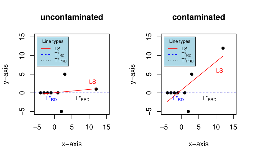
Figure 1: Three regression lines for data without or with contamination (red solid line for LS, blue dashed line for $T^{*}_{RD}$ and black dotted line for $T^{*}_{PRD}$). Left: Original eight-point data set. $T^{*}_{RD}$ and $T^{*}_{PRD}$ are identical. Right: Contaminated data set with one original point moved form $(12,1)$ to $(12,12)$, leading to a drastically change in the LS line while both $T^{*}_{RD}$ and $T^{*}_{PRD}$ are unchanged and resist the contamination.

Regression lines given by the three approaches are plotted w.r.t. the original data versus (i) $12.5\%$ contaminated data set (one data point is contaminated) in Figure 1 left and right and versus (ii) $37.5\%$ contaminated data set (three points out of eight are contaminated) in Figure 2 left and right, respectively.

Inspecting Figure 1, reveals that (i) for the original data, the least squares line is affected by the point with large $x$-coordinate (an outlier in the x-direction, or a leverage point). It is drawn by this leverage point, whereas both deepest regression depth lines resist against the leverage point and capture the horizontal line $y=0$, (ii) When the leverage point is moved upward to $(12,12)$, then the entire least squares line is attracted by this movement and moved upward (which means that a single point can ruin the LS line), whereas both deepest regression depth lines are resistant to this single point contamination. Figure 2, on the other hand, reveals that (i) for the uncontaminated data, the situation is the same as in Figure 1 left, and (ii) for the contaminated data (three points are contaminated), the least squares line again is affected by the leverage point as well as the contaminated points, but not too much from the latter (since the x and y coordinates of the contaminated points are moderate), the deepest line of $T^{*}_{PRD}$ is affected by the contamination but still informative and useful, whereas the one from $T^{*}_{RD}$ is useless (breaks down as expected due to more than $1/3$ of contamination). Note that the RD of this vertical line is $4/8$ while there are other lines that have this depth. To deal with the non-uniqueness problem while in order to have the affine equivariance of the final deepest regression line, one can take an average of lines with the maximum depth. But the resulting line will still have a unbounded slope, hence is useless.

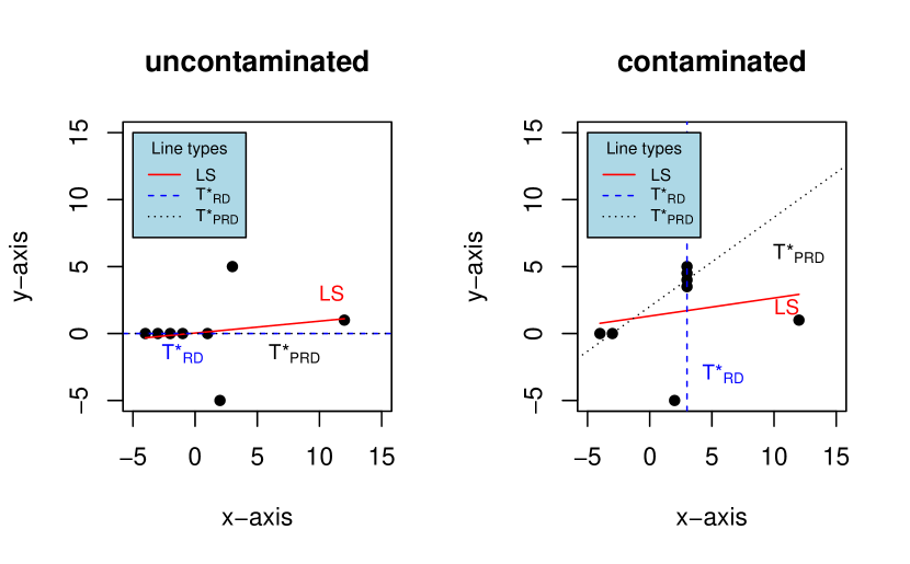
Figure 2: Three regression lines for data without or with contamination (red solid line for LS, blue dashed line for $T^{*}_{RD}$ and black dotted line for $T^{*}_{PRD}$). Left: Original eight-point data set, $T^{*}_{RD}$ and $T^{*}_{PRD}$ are identical. Right: Contaminated data set with three original points moved to the points with 3 as their x-coordinates, $T^{*}_{RD}$ breaks down.

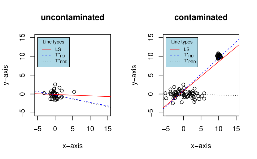
Figure 3: Three regression lines for data without or with contamination (red solid line for LS, blue dashed line for $T^{*}_{RD}$ and black dotted line for $T^{*}_{PRD}$). Left: Original 100 normal points, lines from LS, $T^{*}_{RD}$ and $T^{*}_{PRD}$ are very similar. Right: Contaminated data set with $34\%$ points contaminated, both LS and $T^{*}_{RD}$ “break down” while $T_{PRD}$ resists the contamination and is still useful.

Example 4.2.2.: We generate a bivariate normal data set with size $100$ and $\mu$ and $\Sigma$ are

$$\mu=\begin{pmatrix}0\\ 0\end{pmatrix},~{}~{}~{}~{}\Sigma=\begin{pmatrix}1&-0.8\\ -0.8&1\end{pmatrix};~{}~{}~{}~{}~{}~{}\mu_{1}=\begin{pmatrix}10\\ 10\end{pmatrix},~{}~{}~{}~{}\Sigma_{1}=\begin{pmatrix}0.1&0\\ 0&0.1\end{pmatrix}.$$

Then we consider a $34\%$ replacement normal points contamination with $\mu_{1}$ and $\Sigma_{1}$. The performance of the three lines is displayed in Figure (3).

We compute the three lines w.r.t. un-contaminated data. The three (slope, intercept) lines are (-0.11788718, -0.03614133), (-0.3066041, -0.1899350), and (-0.2943452 -0.2073059) for LS, $T_{RD}$, and $T_{PRD}$, respectively. They do not differ very much as shown in the left side of Figure 3, or all three seem to be useful.On the other hand, we also compute the three lines w.r.t a $34\%$ replacement contamination. The three lines are (0.8283450, 0.7727246), (0.9657038, 0.8559868 ), and (0.03350186, -0.02969263) for LS, $T_{RD}$, and $T_{PRD}$, respectively. They differ very much as shown in the right side of Figure 3. Both LS and $T_{RD}$ lines break down (attached to the cloud of contamination) whereas $T_{PRD}$ can resist the $34\%$ contamination (in fact up to $50\%$) and continue to provide a useful regression line.

4.3 Finite-sample relative efficiency

Robustness does not work in tandem with efficiency. $T^{*}_{PRD}$ (or $T^{*}_{n}$ in the empirical case) has the best possible ABP while it has to pay a price of a relatively low efficiency. Its efficiency, however, could be improved (as shown below) by replacing, the univariate median, the chief source of low efficiency, with a much more efficient depth trimmed or weighted mean (Zuo (2006), Zuo, Cui and He (2004) (ZCH04)) meanwhile keeping it as robust as before, just as its location counterpart, the projection median, does (Zuo (2003)).On the other hand, the deepest regression line in RH99 ($T^{*}_{RD}$) has no such freedom to improve its low efficiency since it is fixed and unlike $T^{*}_{PRD}$, which represents a class of functionals (estimators) with the different choices of univariate functionals $T$ (used in $T^{*}_{PRD}$) that can be highly efficient yet as robust as the univariate median.

In the following we investigate via simulation the finite-sample relative efficiency of the deepest lines $T^{*}_{RD}$ and $T^{*}_{PRD}$ w.r.t. the classical least squares line. We generate $N_{R}$ samples from the simple linear regression model: $y_{i}=\beta_{0}+\beta_{1}x_{i}+e_{i},i=1,2,\cdots,n,$ with different sizes $n$ (see Table 1), where $e_{i}\sim N(0,\sigma^{2})$. In light of the regression equivariance, we can assume w.l.o.g. that $\boldsymbol{\beta}=(\beta_{0},\beta_{1})^{\prime}=(0,0)^{\prime}$. We generate $x_{i}$ from standard normal and $t(2)$ independently with $y_{i}$, which are $N(0,1)$ points. The relative efficiency of the slope and intercept of the lines $T^{*}_{RD}$ and $T^{*}_{PRD}$ w.r.t. those of the least squares line are listed in Table 1 with various $n$, where $T$ in the definition of $T^{*}_{PRD}$ is the sample median.

Inspecting the Table 1 reveals that (i) for Gaussian $x_{i}$’s the intercept of $T^{*}_{RD}$ is slightly more efficient than that of $T^{*}_{PRD}$ when $n\geq 20$, while the slope of $T^{*}_{PRD}$ is more efficient than that of $T^{*}_{RD}$ uniformly for all $n$ , whereas for $t(2)$ $x_{i}$’s, $T^{*}_{PRD}$ is more efficient than $T^{*}_{RD}$ both in slope and intercept uniformly for all $n$; (ii) the efficiency of the deepest regression lines differs when the $x_{i}$ are generated from different distributions; (iii) slopes have higher efficiency for Gaussian $x_{i}^{\prime}s$ than for $t(2)$ $x_{i}^{\prime}s$; and (iv) for Gaussian $x_{i}^{\prime}s$ slopes have higher efficiency than intercept for $n>10$, this relationship is reversed for $t(2)$ $x_{i}^{\prime}s$ for all $n$.

Relative efficiency (based on $N_{R}=5,000$ replications) of the deepest lines $T^{*}_{RD}$ and $T^{*}_{PRD}$ compared to the least squares line when the $x_{i}$ are from Gaussian or $t$ distributions           Gaussian $x_{i}$       t(2) $x_{i}$ n          slope intercept    slope intercept   $(T^{*}_{PRD}$; $T^{*}_{RD})$ $(T^{*}_{PRD}$; $T^{*}_{RD})$ $(T^{*}_{PRD}$; $T^{*}_{RD})$ $(T^{*}_{PRD}$; $T^{*}_{RD})$ 10 (0.6990; 0.6341) (0.7044; 0.6696) (0.6060; 0.5404) (0.6950; 0.6789) 20 (0.7267; 0.7156) (0.6884; 0.6941) (0.6217; 0.6048) (0.7111; 0.7020) 40 (0.7513; 0.7321) (0.7057; 0.7124) (0.6154; 0.5967) (0.7354; 0.7142) 80 (0.7606; 0.7514) (0.7042; 0.7107) (0.5876; 0.5759) (0.7285; 0.7063) 100 (0.7471; 0.7385) (0.7024; 0.7114) (0.5837; 0.5685) (0.7286; 0.7155)

Table 1: Median used for $T$ in $T^{*}_{PRD}$

Relative efficiency (based on $N_{R}=1,000$ replications) of the deepest line $T^{*}_{RD}$ and $T^{*}_{PRD}$ compared to the least squares line when the $x_{i}$ are from Gaussian or $t$ distributions
          Gaussian $x_{i}$       t(2) $x_{i}$ n          slope intercept    slope intercept   $(T^{*}_{PRD}$; $T^{*}_{RD})$ $(T^{*}_{PRD}$; $T^{*}_{RD})$ $(T^{*}_{PRD}$;  $T^{*}_{RD})$ $(T^{*}_{PRD}$; $T^{*}_{RD})$ 10 (0.6496; 0.6065) (0.6780; 0.6676) (0.6561; 0.5874) (0.7070; 0.6930) 20 (0.7196; 0.6982) (0.7346; 0.7316) (0.5813; 0.5582) (0.7311; 0.7010) 40 (0.7581; 0.7289) (0.7784; 0.7655) (0.5972; 0.5722) (0.7207; 0.6869) 80 (0.7816; 0.7482) (0.7177; 0.7054) (0.5992; 0.5686) (0.7323; 0.7098) 100 (0.7505; 0.7462) (0.7166; 0.7138) (0.6201; 0.5978) (0.7065; 0.6931)

Table 2: PWM (see ZCH04) used for $T$ in $T^{*}_{PRD}$

The efficiency of the slope and intercept of the line $T^{*}_{PRD}$ could be improved by replacing median employed in the definition of $T^{*}_{PRD}$ with a more efficient projection depth weighted mean (PWM) yet have the same level of robustness as the median, see Zuo (2003) and Zuo, Cui and He (2004) (ZCH04), and Wu and Zuo (2009):

$$\mbox{PWM}(x^{n})=\frac{\sum_{i=1}^{n}w(PD_{n}(x_{i}))x_{i}}{\sum_{i=1}^{n}w(PD_{n}(x_{i}))},$$

where $w(r)=I(r<c)\big{(}\exp(-k(1-r/c)^{2})-\exp(-k)\big{)}/(1-\exp(-k))+I(r\geq c)$, $PD_{n}(x_{i})=1/(1+|x_{i}-\mbox{Med}(x^{n})|/\mbox{MAD}(x^{n}))$ and $x^{n}=\{x_{1},\cdots,x_{n}\}$ with $x_{i}\in\mathbb{R}$. For discussions of weight function $w$ and parameters $k$ and $c$, see ZCH04. Generally speaking, tuning $c$ to render it smaller to get higher efficiency from PWM. The same is true for parameter $k$. Namely, keeping the number of inner points as large as possible to gain higher efficiency and down-weighting outliers slower to gain higher efficiency. In our simulation, we set $k=3$ and $c=3.5$. Other parameters that could be tuned include $N_{v}$ and $N_{\beta}$ (see Section 4.1). In our simulation, we set $N_{v}=100+2*n$, where $100$ are random directions and $2n$ directions (they are $\mathbf{v_{i}}\pm(10^{-10},0)^{\prime}$, where $\mathbf{w}_{i}^{\prime}\mathbf{v}_{i}=0$, see the RHS of (17), $i=1,\cdots,n$) are strategically chosen. $N_{\beta}$ is increasing with $n$ but no greater than $n(n-1)/2$. With these parameters, the results from $T^{*}_{RD}$ and $T^{*}_{PRD}$ are listed in Table 2. Inspecting Table 2 reveals that (i) with the PWM employed in the definition of $T^{*}_{PRD}$, $T^{*}_{PRD}$ becomes more efficient than $T^{*}_{RD}$ both in slope and intercept uniformly for all $n$ both for Gaussian $x_{i}$ and $t(2)$ $x_{i}$ (note that by tuning the parameters, one can even gets higher efficiency for $T^{*}_{PRD}$). (ii) The efficiency of the deepest lines depends on the distribution of $x_{i}$. (iii) The efficient of the intercept is higher than that of slope for $t(2)$ $x_{i}$’s. This is no longer true for Gaussian $x_{i}$’s and when $n>40$.

5 Discussions and concluding remarks

This article investigates the robustness property of the deepest projection regression depth functional $T^{*}_{PRD}$. $T^{*}_{PRD}$ is closely related to (but different from) the P-estimates in MY93. In fact, it is the modification of the latter, to achieve the scale invariance of the induced depth function and scale equivariance of $T^{*}_{PRD}$.Like MY93 for the P-estimates, an upper bound for the maximum bias of $T^{*}_{PRD}$ is established, which covers Theorems 3.4, 3.5, and 4.1 of MY93. In contrast to MY93 for their P-estimates, the influence function of $T^{*}_{PRD}$ and the finite sample breakdown point of $T^{*}_{n}$ are revealed here as well. The competitor $T^{*}_{RD}$ in RH99 has an advantage over $T^{*}_{PRD}$ in terms of computation in practice, though both confront a challenging computation problem. The computing issue of $T^{*}_{RD}$ has been briefly addressed in RH99 (that of its location counterpart, the halfspace median, has been addressed in Liu, et al (2017), among others). That of $T^{*}_{PRD}$ is yet to be thoroughly investigated elsewhere.$T^{*}_{PRD}$, on the other hand, is superior to $T^{*}_{RD}$ in terms of breakdown point robustness and is not inferior to $T^{*}_{RD}$ in terms of relative efficiency.

Acknowledgments

The author thanks Professor Emeritus James Stapleton for his careful English proofreading and an anonymous referee who provided insightful comments and suggestions which have led to significant improvements of the manuscript.

References

• [1] Adrover, J. and Yohai, V.ย J. (2002), โ€œProjection estimates of multivariate locationโ€, Ann. Statist., 30 1760-1781.
• [2] Bai,Z.ย D.โ€‰ and He, X. (1999), โ€œAsymptotic distributions of the maximal depth regression and multivariate locationโ€, Ann. Statist., Vol. 27, No. 5, 1616โ€“1637. 577-580.
• [3] Chen, Z. and Tyler, D.ย E. (2002), โ€œThe influence function and maximum bias of Tukeyโ€™s medianโ€, Ann. Statist., 30 1737-1759.
• [4] Davies, P. L. (1990), โ€œThe asymptotics of S-estimators in the linear regression modelโ€, Ann. Statist., 18 1651-1675.
• [5] Davies, P. L. (1993), โ€œAspects of robust linear regressionโ€, Ann. Statist., 21 1843-1899.
• [6] Davies, P.ย L., and Gather, U.ย (2005), โ€œBreakdown and groupsโ€, Ann. Statist., Vol. 33, No. 3, 977-988.
• [7] Donoho, D.ย L.ย (1982), โ€œBreakdown properties of multivariate location estimatorsโ€, PhD Qualifying paper, Harvard Univ.
• [8] Donoho, D. L. and Huber, P. (1983), In A Festschrift for Erich L. Lehmann, 157โ€“-184. Wadsworth, Belmont, CA.
• [9] Hampel, F.ย R., Ronchetti, E.ย M., Rousseeuw, P.ย J., and Stahel, W.ย A. (1986), Robust Statistics: The Approach Based on Influence Functions, John Wiley & Sons, New York.
• [10] Huber, P.ย J.ย (1964), โ€œRobust estimation of a location parameterโ€, Ann. Math. Statist., 35 73-101
• [11] Huber, P.ย J.ย (1972), โ€œRobust statistics: A reviewโ€, Ann. Math. Stat., 43, 1041-1067.
• [12] Huber, P.ย J. (1981), Robust Statistics, Wiley, New York.
• [13] Hubert, M., Rousseeuw, P. J. and Van Aelst, S. (2001), โ€œSimilarities between location depth and regression depthโ€. In Statistics in Genetics and in the Environmental Sciences (L. Fernholz, S. Morgenthaler and W. Stahel, eds.) 159-172. Birkhรคuser, Basel.
• [14] Kim, J. and Pollard, D. (1990). โ€œCube root asymptoticsโ€. Ann. Statist., 18 191โ€“219.
• [15] Koenker, R., and Bassett, G.ย J.ย (1978), โ€œRegression Quantilesโ€, Econometrica, 46, 33โ€“50.
• [16] Liu, X., Luo, S. & Zuo, Y. (2017), โ€œSome results on the computing of Tukeyโ€™s halfspace medianโ€, Stat Papers, https://doi.org/10.1007/s00362-017-0941-5.
• [17] Maronna, R.ย A.,ย and Yohai, V.ย J.ย (1993), โ€œBias-Robust Estimates of Regression Based on Projectionsโ€, Ann. Statist., 21(2), 965-990.
• [18] Martin, D.ย R., Yohai, V.ย J., and Zamar, R.ย H. (1989), โ€œMinโ€“max bias robust regressionโ€, Ann. Statist., 17 1608-1630.
• [19] Mรผller, C. (2013), โ€œUpper and lower bounds for breakdown pointsโ€. In: Becker C, Fried R, Kuhnt S (eds) Robustness and complex data structures. Festschrift in Honour of Ursula Gather. Springer, Berlin, pp 17-34.
• [20] Rousseeuw, P.ย J. (1984), โ€œLeast Median of Squares Regression,โ€ J. Amer. Statist. Assoc., 79, 871โ€“880.
• [21] Rousseeuw, P.ย J., and Hubert, M. (1999), โ€œRegression depthโ€ (with discussion), J. Amer. Statist. Assoc., 94: 388โ€“433.
• [22] Rousseeuw, P.J., and Leroy, A. (1987), Robust regression and outlier detection. Wiley New York, 1987.
• [23] Seber, G. A. F. and A. J. Lee (2003), Linear Regression Analysis, Second Edition, John Wiley & Sons, Inc., Hoboken, New Jersey.
• [24] Shao, W. and Zuo, Y. (2018), โ€œComputing the halfspace depth with multiple try algorithm and simulated annealing algorithmโ€, Computational Statistics (in press).
• [25] Tukey, J.ย W. (1975), โ€œMathematics and the picturing of dataโ€, In: James, R.D. (ed.), Proceeding of the International Congress of Mathematicians, Vancouver 1974 (Volume 2), Canadian Mathematical Congress, Montreal, 523-531.
• [26] Van Aelst, S., and Rousseeuw, P.ย J. (2000), โ€œRobustness of Deepest Regressionโ€, J. Multivariate Anal., 73, 82โ€“106.
• [27] Wu, M., and Zuo, Y. (2008), โ€œTrimmed and Winsorized Standard Deviations based on a scaled deviationโ€, Journal of Nonparametric Statistics, 20(4), 319-335.
• [28] Wu, M., and Zuo, Y. (2009), โ€œTrimmed and Winsorized means based on a scaled deviationโ€, J. Statist. Plann. Inference, 139(2), 350-365.
• [29] Zuo, Y. (2003) โ€œProjection-based depth functions and associated mediansโ€, Ann. Statist., 31, 1460-1490.
• [30] Zuo, Y. (2006), โ€œMulti-dimensional trimming based on projection depthโ€, Ann. Statist., 34(5), 2211-2251.
• [31] Zuo, Y., Cui, H. and He, X. (2004a), โ€œOn the Stahel-Donoho estimator and depth-weighted means of multivariate dataโ€, Ann. Statist., 32(1): 167-188.
• [32] Zuo, Y., Cui, H. and Young, D. 2004, โ€œInfluence function and maximum bias of projection depth based estimatorsโ€, Ann. Statist., 32, 189-218.
• [33] Zuo, Y. (2018), โ€œOn general notions of depth in regressionโ€, arXiv:1805.02046.