Fundamental limits of detection in the spiked Wigner model
Abstract
We study the fundamental limits of detecting the presence of an additive rank-one perturbation, or spike, to a Wigner matrix. When the spike comes from a prior that is i.i.d. across coordinates, we prove that the log-likelihood ratio of the spiked model against the non-spiked one is asymptotically normal below a certain reconstruction threshold which is not necessarily of a “spectral” nature, and that it is degenerate above. This establishes the maximal region of contiguity between the planted and null models. It is known that this threshold also marks a phase transition for estimating the spike: the latter task is possible above the threshold and impossible below. Therefore, both estimation and detection undergo the same transition in this random matrix model. We also provide further information about the performance of the optimal test. Our proofs are based on Gaussian interpolation methods and a rigorous incarnation of the cavity method, as devised by Guerra and Talagrand in their study of the Sherrington–Kirkpatrick spin-glass model.
1 Introduction
Spiked models, which are distributions over matrices of the form “signal + noise,” have been a mainstay in the statistical literature since their introduction by Johnstone, (2001) as models for the study of high-dimensional principal component analysis. Spectral properties of these models have been extensively studied, in particular in random matrix theory, where they are known as deformed ensembles (Péché, , 2014). Landmark investigations in this area (Baik et al., , 2005; Baik and Silverstein, , 2006; Péché, , 2006; Féral and Péché, , 2007; Capitaine et al., , 2009; Bai and Yao, , 2012, 2008) have established the existence of a spectral threshold above which the top eigenvalue detaches from the bulk of eigenvalues and becomes informative about the spike, and below which the top eigenvalue bears no information. Estimation using the top eigenvector undergoes the same transition, where it is known to “lose track” of the spike below the spectral threshold (Paul, , 2007; Nadler, , 2008; Johnstone and Lu, , 2009; Benaych-Georges and Nadakuditi, , 2011). Although these spectral analyses have provided many insights, as have analyses based on more thoroughgoing usage of spectral data and/or more advanced optimization-based procedures (see Ledoit and Wolf, , 2002; Amini and Wainwright, , 2009; Berthet and Rigollet, , 2013; Dobriban, , 2017, and references therein), they do not characterize the fundamental limits of estimating the spike, or detecting its presence, from the observation of a sample matrix. Important progress on the detection problem was made by Onatski et al., (2013, 2014) and Johnstone and Onatski, (2015), who considered the spiked covariance model for a uniformly distributed unit norm spike, and studied the asymptotics of the likelihood ratio (LR) of a spiked alternative against a spherical null. They showed asymptotic normality of the log-LR below the spectral threshold (also known as the BBP threshold, after Baik et al., , 2005, in this setting), while it is degenerate, i.e., exponentially small (large) under the null (alternative), above it. Their proof is intrinsically tied to the assumption of a spherical prior since it relies on the rotational symmetry of the model to express the LR exclusively in terms of the spectrum, the joint distribution of which is available in closed form.
We focus in this paper on the spiked Wigner model, which is the following symmetric random matrix model:
| (1) |
where and , , are independent for all . The spike vector represents the signal to be recovered, or its presence detected.
We assume that the entries of the spike are i.i.d. from a prior distribution on having bounded support. The parameter plays the role of the signal-to-noise ratio, and the scaling by is such that the signal and noise components of the observed data are of comparable magnitudes. Upon observing , we want to test whether or . We moreover want to understand the performance of the likelihood ratio test, which minimizes the sum of the Type-I and Type-II errors by the Neyman-Pearson lemma.
The testing problem becomes more subtle in our setting, where the spike comes from a product prior, since it is not clear that one does not lose power by discarding the eigenvectors of . In fact, this situation presents a richer phenomenology: while the spherical case is characterized by the behavior of the spectrum, and the spectral threshold separates the regions of convergence and degeneracy of the LR, there are priors in the i.i.d. case for which the spectral threshold loses its information-theoretic relevance. These priors exhibit a more subtle phase transition that happens strictly before the spike manifests its presence in the spectrum. A desire to understand this phenomenon is the main impetus for the present work.
This transition was discovered by Lesieur et al., (2015) while studying the estimation problem in the context of sparse PCA. Perry et al., (2016) and Banks et al., (2017) proved the possibility of both estimation and asymptotically certain—we will say “strong”—detection below the spectral threshold for certain sparse priors. However, their techniques—which are based on careful conditioning of the second moment of the LR—are not able to determine the phase transition threshold, the explicit form of which was conjectured by Lesieur et al.
Our contribution is to rigorously pin down this phase transition for the detection problem. We prove asymptotic normality of the log-LR below a certain reconstruction threshold and degeneracy above it. This allows us to show mutual contiguity of the null and the alternative below and to derive formulas for the Type-I and Type-II errors of the LR test, as well as the KL divergence and total variation distance, between the null and alternative. Our approach reposes on seminal work by Guerra and Talagrand in their study of the Sherrington-Kirkpatrick (SK) spin-glass model.
The paper is organized as follows: Section 2 sets up the problem, Section 3 contains our main results on LR fluctuations and the limits of detection, Section 4 provides background on essential concepts from spin-glass theory that are necessary for the proof, and Sections 5, 6 and 7 are devoted to the detailed proofs.
2 The LR, the formula and the reconstruction threshold
2.1 The LR
We denote by the joint probability law of the observations, , as per (1) and we define the likelihood ratio or Radon-Nikodym derivative of with respect to as
| (2) |
Conditioning on and using the Gaussianity of yields the formula
| (3) |
for any fixed . Define the free energy of the planted model as
| (4) |
where is the Kullback-Leibler divergence between probability measures. The reconstruction threshold is defined as the largest positive number below which the limit of vanishes. This latter limit, referred to as the replica-symmetric () formula, provides a full characterization of the limits of estimating the spike with non-trivial accuracy (Barbier et al., , 2016; Lelarge and Miolane, , 2016).
2.2 The formula
For , consider the function
| (5) |
where , and . This is the divergence between the distributions of the random variables and . We define the replica-symmetric potential
| (6) |
and the replica-symmetric formula
| (7) |
A central result in this context, which was conjectured by Lesieur et al., (2015), and then proved in a sequence of papers (Deshpande et al., , 2016; Barbier et al., , 2016; Krzakala et al., , 2016; Lelarge and Miolane, , 2016; El Alaoui and Krzakala, , 2018), is that free energy converges to the formula for all :
| (8) |
In particular the limit is independent of , i.e., it is insensitive to .
The values of that maximize the potential and their properties play an important role. Lelarge and Miolane, (2016) proved that the map has a unique maximizer for all where . Moreover, they showed that the map is non-decreasing, and
| (9) |
where . One can interpret the value as the best overlap an estimator based on observing can have with the spike . Indeed, Lelarge and Miolane also showed that the squared overlap between the spike and a random draw from the posterior concentrates about .
2.3 The reconstruction threshold
The first limit in (9) shows that when the prior is not centered, it is always possible to have a non-zero overlap with (just by guessing at random from the prior). An interesting situation then is when the prior has zero mean. Since is a non-decreasing function of , it is useful to define the critical value of below which a non-zero overlap with is impossible:
| (10) | ||||
The second equality follows by the a.e. uniqueness of the maximizer . We refer to as the reconstruction threshold. The next lemma establishes a natural bound on .
Lemma 1.
We have .
Proof.
Indeed, assume that is centered, and let . Since and , we see that and . So cannot be a maximizer of . Therefore and .
The importance of Lemma 1 stems from the fact that the value is the spectral threshold previously discussed. Above this value, the first eigenvalue of the matrix detaches from the bulk (Péché, , 2006; Capitaine et al., , 2009; Féral and Péché, , 2007). This value also marks the limit below which the first eigenvector of captures no information about the spike (Benaych-Georges and Nadakuditi, , 2011). The inequality in Lemma 1 can be strict or turn into equality depending on the prior . For instance, there is equality if the prior is Gaussian or Rademacher—so that the first eigenvector overlaps with the spike as soon as estimation becomes possible at all—and strict inequality in the case of the (sufficiently) sparse Rademacher prior . More precisely, there exists a value
such that for , and for . In the latter case, the spectral approach to estimating fails for , and it is believed that no polynomial time algorithm succeeds in this region (Lesieur et al., , 2015; Krzakala et al., , 2016; Banks et al., , 2017).
3 Fluctuations below the reconstruction threshold
In this section we study the behavior of . It can be seen by a standard concentration-of-measure argument that for all , concentrates about its expectation with fluctuations of order . While this bound is likely to be of the right order above , it is very pessimistic below . Indeed, we will show that the fluctuations are of constant order with a Gaussian limiting law in this regime. This behavior of unusually small fluctuations is often referred to as “super-concentration.” We refer to Chatterjee, (2014) for more on this topic. Throughout the rest of the paper, except in Section 8, we discard the diagonal terms from the observations: we formally take in (3). (See the Remark below).
Theorem 2.
Assume that the prior is centered, has unit variance and bounded support. Also, let . For all ,
where the plus sign holds under the alternative and the minus sign under the null . The symbol denotes convergence in distribution as .
Remark.
The assumption is only for convenience; its removal does not pose any additional technical difficulties. When the diagonal is kept, the limiting Gaussian is still of the form , but now , . We refer to Section 8 for a discussion of how this adjusted formula would appear in the proof.
We point out that a result of this form was originally proved in the case of the Sherrington–Kirkpatrick (SK) model: Aizenman et al., (1987) showed that the log-partition function of this model has Gaussian fluctuations in the “high temperature” regime (which corresponds to small enough.) In fact, Theorem 2, if specialized to the Rademacher prior , reduces to their result (with ) since the LR is equal to the partition function of the SK model in that case.
Our result has a parallel in the work of Johnstone and Onatski, (2015); Onatski et al., (2013, 2014), who focused on sperical priors and studied the likelihood ratio of the joint eigenvalue densities under the spiked covariance model, showing its asymptotic normality below the spectral threshold. We also note that similar fluctuation results were recently proved by Baik and Lee, (2016, 2017) for a spherical model where one integrates over the uniform measure on the sphere in the definition of . Their model, due to its integrable nature, is amenable to analysis using tools from random matrix theory. The authors are thus able to also analyze a “low temperature” regime (absent from our problem) where the fluctuations are no longer Gaussian but given by the Tracy-Widom distribution. However, their techniques seem to be restricted to the spherical case. Closer to our setting is the recent work of Banerjee and Ma, (2018) (see also Banerjee, , 2018) who use a very precisely conditioned second-moment argument to show asymptotic normality of similar log-likelihood ratios. However, this technique (at least in its current state) is not able to achieve the optimal threshold .
3.1 Limits of strong and weak detection
Consider the problem of deciding whether an array of observations is likely to have been generated from for a fixed or from . Let us denote by the null hypothesis and the alternative hypothesis. Two formulations of this problem exist: one would like to construct a sequence of measurable tests that returns “0” for and “1” for , for which either
| (11) |
or less stringently, the total mis-classification error, or risk,
| (12) |
is minimized among all possible tests .
Strong detection
Using a second-moment argument (based on the computation of a truncated version of ), Banks et al., (2017) and Perry et al., (2016) showed that and are mutually contiguous when , where the latter quantity equals for some priors while it is suboptimal for others (e.g., the sparse Rademacher case; see further discussion below). It is easy to see that contiguity implies impossibility of strong detection since, for instance, if then . Here we show that Theorem 2 provides a more powerful approach to contiguity:
Corollary 3.
Assume the prior is centered, has unit variance and bounded support. Then for all , and are mutually contiguous.
Proof.
This approach allows one to circumvent second-moment computations which are not guaranteed to be tight in general, and necessitate careful and prior-specific conditioning that truncates away problematic atypical events. On the other hand, we show that strong detection is possible above (the proof is at the end of the paper):
Proposition 4.
Let . If , then with probability approaching one as . On the other hand, if then with probability approaching one as . Therefore and are mutually orthogonal above .
Remark.
It is tempting to believe that above (the high-probability statement is then a consequence of concentration), but we do not know of a simple proof of this. One can show, following Guerra, (2003), that there is a non-increasing sequence of thresholds —each one corresponding to the point where the so-called “-” interpolation bound dips below zero—such that the above limit is strictly negative above . By our contiguity argument, it is necessarily true that . Equality would follow if one can show overlap convergence (the analogue of Theorem 10 with replacing ) for all under the null model , but this goes beyond the scope of this paper.
Weak detection
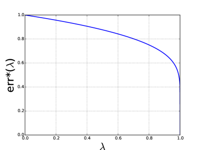
We have seen that strong detection is possible if and only if . It is then natural to ask whether weak detection is possible below ; i.e., is it possible to test with accuracy better than that of a random guess below the reconstruction threshold? The answer is yes, and this is another consequence of Theorem 2. More precisely, the optimal test minimizing the risk (12) is the likelihood ratio test which rejects the null hypothesis (i.e., returns “1”) if , and its error is
| (13) |
One can readily deduce from Theorem 2 the Type-I and Type-II errors of the likelihood ratio test. By symmetry of the means of the limiting Gaussians, the errors and converge to a common limit for all , where and is the complementary error function. Therefore, one obtains the following formula for and the total variation distance between and (ploted in Figure 1):
Corollary 5.
For all (and ), we have
| (14) |
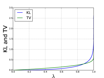
Moreover, the proof of Theorem 2 allows us to obtain a formula for the divergence between and below the reconstruction threshold (see Figure 1):
Corollary 6 (of the proof).
Assume the prior is centered, is of unit variance and has bounded support (and .) Then for all ,
| (15) |
Note that the above formulas are only valid up to . When , and both witness an abrupt discontinuity at to 1 and respectively. When , then the behavior is more smooth with an asymptote at .
4 Replicas, overlaps, Gibbs measures and Nishimori
4.1 Important notions
A crucial component of the proof of our main results is the understanding of the convergence of the overlap , where is drawn from , to its limit . By Bayes’ rule, we see that
| (16) |
where is the Hamiltonian (recall that )
| (17) |
From the equations (3) and (4), it is straightforward to see that
This provides another way of interpreting as the expected log-partition function (or normalizing constant) of the posterior . For an integer and , we define the Gibbs average of w.r.t. as
| (18) |
This is simply the average of with respect to . The variables , are called replicas, and are interpreted as random variables drawn independently from the posterior. When we simply write instead of . Throughout this paper, we use the following notation: for , we let
4.2 The Nishimori property under
The fact that the Gibbs measure is a posterior distribution (16) has far-reaching consequences. A crucial implication is that the -tuples and have the same law under . To see this, let us perform the following experiment:
-
1.
Construct by independently drawing its coordinates from .
-
2.
Construct as , where are all independent for . (Therefore, is distributed according to .)
-
3.
Draw independent random vectors from .
By the tower property of expectations (for a three-line proof, see Proposition 16, Lelarge and Miolane, , 2016), the following equality of joint laws holds
| (19) |
This implies in particular that under the alternative , the overlaps between a replica and the spike have the same distribution as the overlap between two replicas. The latter is a very important property of the planted model , which is usually named after Nishimori, (2001) in spin-glass theory. Property (19) substantially simplifies important technical arguments that are otherwise very difficult to conduct under the null. A recurring example in our context is the following: to prove the convergence of the overlap between two replicas, , it suffices to prove since the two quantities are equal.
5 Proof of LR fluctuations
In this section we prove Theorem 2. It suffices to prove the fluctuations under one of the hypotheses. Fluctuations under the remaining one come for free as a consequence of Le Cam’s third lemma (Van der Vaart, , 2000, Theorem 6.6). We choose to treat the planted case . The reason is that it is easier to deal with the planted model, due to the Nishimori property (19).
5.1 Fluctuations under
In this section we prove Gaussian fluctuations of through the convergence of its characteristic function. Let and be fixed. For and , let
Theorem 7.
For all and , there exists a constant such that
where .
The map is the characteristic function of .
Lemma 8.
For all ,
| (20) |
Proof.
By differentiation with respect to we obtain
where the Hamiltonian is given in (17). Since , we can write more explicitly . Therefore
| (21) | ||||
Now we perform Gaussian integration by parts with respect to each variable and obtain
Plugging this into (21) and rearranging, we obtain
| (22) | ||||
Since we are under the planted model and depends only on , we can use the Nishimori property (19) to replace and by and respectively in the first term of (22).
The derivative involves the average . A crucial step in the argument is to show that and its pre-factor in the above expression are asymptotically independent, so that one can split the expectation of the product into the product of the expectations. More precisely, one should expect the quantities and to tightly concentrate about some deterministic values when , such that the second expectation in (20) is a multiple of . We will then be left with a simple differential equation whose solution is .
Proposition 9.
For all and , there exists such that
where .
From here, we can prove the convergence of by integrating the differential equation given in Lemma 8.
Proof of Theorem 7. Plugging the result of Proposition 9 into Lemma 8 yields
where . Since and the primitive of is , integrating w.r.t. yields the result.
Proof of Corollary 6. We prove the convergence of . By differentiation and use of the Nishimori property (19), we have
Now we use Proposition 9 with , and integrate w.r.t. to conclude.
It remains to prove Proposition 9. This will require the deployment of techniques from the theory of mean-field spin glasses.
5.2 Sketch of proof of Proposition 9
The idea is to show self-consistency relations among the quantities of interest. Namely, we will prove that for all ,
| (23) |
and
| (24) |
where in both cases
Next, we need to prove the convergence of the third moment of the overlap under at an optimal rate of :
Theorem 10.
For all , there exists a constant such that
6 Proof of asymptotic decoupling
We proceed to the proof of Proposition 9. As explained earlier, the argument is in two stages. We first prove (23) then (24).
6.1 Preliminary bounds
We make repeated use of interpolation arguments in our proofs. We state here a few elementary lemmas that we will invoke several times. We denote the overlaps between replicas where the last variable is deleted by a superscript “-”:
Let be a family of interpolating Hamiltonians. We let denote the corresponding Gibbs average, similarly to (18). Following Talagrand’s notation, we write
for a generic function of replicas , . We abbreviate by . The main tool we use is the following interpolation that isolates the last variable from the rest of the system:
| (25) | ||||
At we have , and at the variable decouples from the rest of the variables. Moreover, the Nishimori property (19) is still valid under : the last column of simply becomes .
Lemma 11.
let be a function of replicas and . Then
where we have written .
Proof.
The computation relies on Gaussian integration by parts. See Talagrand, 2011a , Lemma 1.6.3, for the details of a similar computation.
Lemma 12.
If is a bounded nonnegative function, then for all ,
Proof.
Since the variables and the overlaps are all bounded, using Lemma 11 we have for all
Then we conclude using Grönwall’s lemma.
6.2 The cavity method
In its essence, the cavity method amounts to removing one variable from the system—in a manner akin to leave-one-out methods in statistics—and analyzing the influence of the remaining variables on the variable that has been removed. It was initially introduced to solve certain models of spin glasses (Mézard et al., , 1990), and was developed into a rigorous probabilistic theory by Talagrand, 2011a ; Talagrand, 2011b . To make use of the cavity method, we isolate the th variable from the rest (without loss of generality, by symmetry among the variables ) and compute:
Let
where is defined in (25). Note that we have . We now consider the interpolative function
Our strategy is approximate by via a Taylor expansion, which requires is to control the second derivative . Notice that since the last variable decouples from the rest of the system at , we have
The latter equality holds since is centered. Next, a bit of algebra (similarly to Lemma 11) shows that the derivative is a linear combination of terms of the form
| (26) |
where . We see that at , if the above expression involves a variable of degree 1 then this term vanishes. Therefore the only remaining term is the one where . Therefore
| (27) | ||||
The last equality holds since has unit variance. Now we turn to . Taking another derivative generates monomials of degree three in the overlaps and the last variable, so is a linear combination of terms
| (28) |
where range over a finite set of combinations. Our goal is to bound the second derivative independently of , so that we are able to use the Taylor approximation
| (29) |
Since has bounded support and , Hölder’s inequality and the Nishimori property imply that (28) is bounded in modulus by
Using Lemma 12 and the convergence of the fourth moment, Theorem 10, we have
Therefore by the above estimates we have
| (30) |
Now, our next goal is to prove
| (31) |
We consider the function
Observe that (27) tells us that . On the other hand,
By boundedness of the prior, the first term in the RHS is bounded by
and the second term is bounded by . So it suffices to show that
Similarly to , the derivative of is a sum of terms of the form
It is clear that the same method used to bound (the generic term of which is (28)) also works in this case, so we obtain the desired bound on . Finally, using (29), (30) and (31), we obtain
where . This is equivalent to (23) and closes the first stage of the argument. Now we need to show that
We similarly consider the function . We have
The derivative of is a sum of term of the form
By our earlier argument, for all , so that
It remains to show that , and this is done in exactly the same way: by bounding the derivative of . This yields (24) and concludes the proof.
7 Overlap convergence
In this section we prove Theorem 10 on the convergence of the overlaps to zero under , and below . At a high level, we will first prove that the overlap converges in probability to zero under : for all ,
| (32) |
This will be achieved via two interpolation bounds combined with concentration of measure. The way the argument works is roughly as follows: for a fixed we have
We invoke concentration-of-measure arguments to show that the logarithmic terms in the numerator and the denominator are close to their expectations, hence we obtain
where and is the unconstrained free energy (with no indicator). It is now apparent that is exponentially unlikely to take values such that . It remains to lower bound and upper bound by quantities that preserve a strict inequality for all . These quantities will naturally be the replica-symmetric formula and the replica-symmetric potential respectively, and the proof relies on Guerra’s interpolation method.
Next, this convergence in probability is boosted to a statement of convergence of the second moment: , which is in turn boosted to a statement of convergence of the fourth moment: . The apparent recursive nature of this argument is a feature of the cavity method: one can control higher-order quantities once one knows how to control low-order ones and control certain error terms. We now present the interpolation bounds and then prove (32). The cavity arguments which allow us to convert this to convergence of moments are presented in Appendices A and B, since they are very similar to the arguments already presented in Section 6.
7.1 Guerra’s interpolation bound
We present the interpolation method of Guerra, (2001); a main tool in our arguments.
Proposition 13.
Recall . For all , there exist such that
Proof.
Consider the family of interpolating Hamiltonians
| (33) | ||||
where the ’s are i.i.d. standard Gaussian r.v.’s independent of everything else, and . We similarly define the Gibbs average as in (18) where is replaced by . Note that the Nishimori property (19) is preserved under for all . Indeed, the interpolation is constructed in such a way that is the posterior distribution of the signal given the augmented set of observations
| (34) |
which can be interpreted as having side information about from a scalar Gaussian channel with . Now we consider the interpolating free energy
| (35) |
We see that and . This function is differentiable in , and by differentiation, we have
Now we use Gaussian integration by parts to eliminate the variables and . The details of this computation are explained extensively in many sources (see, e.g., Talagrand, 2011a, ; Krzakala et al., , 2016; Lelarge and Miolane, , 2016). We get
Completing the squares yields
| (36) | ||||
The first line in the above expression involves overlaps between two independent replicas, while the second one involves overlaps between one replica and the planted solution. Using the Nishimori property, the derivative of can be written as
| (37) |
The last term follows by symmetry between variables. We finish the argument by noting that , and the product is bounded, we then integrate with respect to time to obtain the result.
7.2 Guerra’s interpolation at fixed overlap
Let us first introduce the so-called Franz-Parisi (FP) potential (Franz and Parisi, , 1995, 1998). For fixed, and define the set
Now define the FP potential as
| (38) |
where the expectation is only over the Gaussian disorder . This is the free energy of a subsystem of configurations having an overlap close to a fixed value with the planted signal .
For and , we let
| (39) |
and
| (40) |
We see that , but unlike , the function does not have an interpretation as the between two distributions. The next lemma states a key property of this function that will be useful later on (see Appendix C for the proof):
Lemma 14.
For all , .
Proposition 15.
Fix , and . There exist constants such that
Proof.
To obtain a bound on we use the interpolation method with Hamiltonian
by varying . The r.v.’s are all i.i.d. standard Gaussians independent of everything else. We define
We compute the derivative w.r.t. , and use Gaussian integration by prts to obtain
where is the Gibbs average w.r.t. the Hamiltonian . A few things now happen. Notice that the planted term (first term in the second line) is trivially smaller than due to the overlap restriction. Moreover, the last terms in both lines are of order since the variables are bounded. The first term in the first line, which involves the overlap between two replicas, is more challenging. What makes this term difficult to control is that the Gibbs measure no longer satisfies the Nishimori property due to the overlap restriction, so the overlap between two replicas no longer has the same distribution as the overlap of one replica with the planted spike. Fortunately, this term is always non-positive so we can ignore it altogether and obtain an upper bound:
Integrating over , we get
Finally, by dropping the indicator, we have
7.3 Convergence in probability of the overlaps
Proposition 16.
For all and , there exist constants such that
To prove the above proposition we first show that the partition function of the model enjoys sub-Gaussian concentration on a logarithmic scale. This is an elementary consequence of two classical concentration-of-measure results: concentration of Lipschitz functions of Gaussian random variables, and concentration of convex Lipschitz functions of bounded random variables.
Lemma 17.
Fix and let be a Borel subset of . Define the random variable
where the randomness comes from the Gaussian disorder . There exists a constant depending on and such that for all ,
Proof.
We notice that the map is Lipschitz with constant for every . Then we invoke the Borell-Tsirelson-Ibragimov-Sudakov inequality of concentration of Lipschitz functions of Gaussian r.v.’s. See Boucheron et al., (2013).
Lemma 18.
Define the random variable
where the randomness comes from the planted vector . There exist a constant depending on and such that for all ,
Proof.
We notice that the map is Lipschitz with constant and convex. Moreover, the coordinates are bounded. We then invoke Talagrand’s inequality on the concentration of convex Lipschitz functions of bounded r.v.’s. See Boucheron et al., (2013).
Lemma 19.
There exists a constant depending on and such that for all ,
Proof.
Since , and , where is a bound on the radius of the support of , we have . The claim now follows from Hoeffding’s inequality.
Proof of Proposition 16. For , we can write the decomposition
where the integer index ranges over a finite set of size since the prior has bounded support. We will only treat the first sum in the above expression since the argument extends trivially to the second sum. Let and write
| (41) |
By virtue of Lemma 17 the two quantities in this fraction enjoy sub-Gaussian concentration on a logarithmic scale over the Gaussian disorder. For any given and , we simultaneously have
and
with probability at least . On the complement of this event, we simply bound the fraction in (41) by 1. Combining the above bounds we obtain
where
with . By Proposition 15, is upper-bounded by a quantity that concentrates over the randomness of . We use Lemma 18 and Lemma 19 in the same way we used Lemma 17: for , we simultaneously have
and
with probability at least , where
Moreover, by Lemma 14, we have . Therefore
The second term is obtained by considering the low-probability complement event and noting that . Now, by Proposition 13, . When , is the unique maximizer of the potential. Therefore for all . We obtain
Finally, adjusting the parameters yields the desired result (e.g., and ).
Proof of Proposition 4. Here we prove possibility of strong detection above . From Proposition 13, we know that for . On the other hand, by Jensen’s inequality. Now it remains to argue that concentrates about its expectation under both and . This is a consequence of Lemmas 17 and 18: we have, for all ,
This concludes the proof. (Note also that the tail decays fact enough to insure almost-sure convergence via the Borel-Cantelli lemma.)
8 When the diagonal is not discarded
When the variance of the diagonal noise entries is kept finite, one has to keep track of the contribution of the diagonal part of the Hamiltonian. In this case, the derivative of the characteristic function of the log-LR w.r.t. displayed in Lemma 8 has an additional term:
The cavity computations performed in Section 6 also need to be altered in a minor way: in the interpolation argument separating the last variable from the rest of the variables, we also have to make time-dependent by performing the change of variable . As a result of the computation, Equation (23) becomes
with , , while Equation (24) remains intact. As a result of these changes, and the above formula for , we get
and this leads to the formula claimed.
9 Conclusion
This paper investigates the fundamental limits of spike detection in the rank-one spiked Wigner model. We proved that the logarithm of the likelihood ratio has Gaussian fluctuations below the reconstruction threshold while it is exponentially large under the alternative above it. This establishes the maximal region of contiguity between the planted and null models: namely the open interval . This also pins down the performance of the optimal test, and provides formulae for the Kullback-Leibler and the total variation distances between the null and planted distributions. An important characteristic of this threshold is that it is not necessarily related to the spectrum of the observed matrix: there are cases where does not correspond to the point where the signal shows up in the spectrum.
Our proofs repose on the technology developed within spin-glass theory for the study of the SK model. It is of interest to extend these techniques to other spiked models, notably spiked covariance models where the perturbation is in the covariance matrix of the data. Partial progress establishing Gaussian fluctuations of the LR in a restricted regime was recently obtained by a subset of the authors (El Alaoui and Jordan, , 2018). Reaching the optimal threshold—a conjectural formula of which is provided in this recent paper—remains an interesting problem.
Appendix A Convergence of the second moment
In this section we prove the convergence of the second moment of the overlaps: . We recall the notation , where denotes the interpolating Gibbs average corresponding to the Hamiltonian
The following lemma will be useful.
Lemma 20.
For all , and all such that ,
| (42) | ||||
| (43) |
Proof.
By symmetry between variables, we have
By the first bound (42) of Lemma 20 with , , we have
with . On the other hand, by the second bound (43) with , , we get
This is because , since last variable decouples from the remaining variables under the measure . Now, we use Lemma 11 with , to evaluate the above derivative at . We still write .
In the above, the only term that survived is the second one since all variables appearing in it are squared. We now use Lemma 20 to argue that . We apply the estimate (42) with , and to obtain
with . Moreover,
The third term is of order , and the second term is bounded by . Therefore
with
Putting things together, we have proved that
| (44) |
where
| (45) |
Now we need to control the error term . By elementary manipulations,
and
Therefore, from (45) we have
| (46) |
At this point, the prior knowledge that is small with high probability is useful. It implies that and . With Proposition 16 we have for
and
Combining the above two bounds with (46), and then injecting in (44), we get
We choose small enough and large enough that . We obtain
Appendix B Convergence of the fourth moment
In this section we prove the convergence of the fourth moment: . We adopt the same technique based on the cavity method, with the extra knowledge that the second moment converges. Many parts of the argument are exactly the same so we will only highlight the main novelties in the proof. By symmetry between variables,
The quadratic term is bounded as
The last inequality is using our extra knowledge about the convergence of the second moment. The last two terms are also bounded by and respectively. Now we must deal with the cubic term, and here, we apply the exact same technique used to deal with the term in the previous proof. The argument applies verbatim and we obtain
Using Proposition 16, we have for ,
Now, we finish the argument in the same way, by choosing sufficiently small. This concludes the proof of Theorem 10.
Appendix C Proof of Lemma 14
A straightforward calculation reveals that
so that is Lipschitz and strongly convex on any interval, and for all .
Let , and let be the symmetric part of , i.e., for all Borel . We observe that is absolutely continuous with respect to , so that the Radon-Nikodym derivative is a well-defined measurable function from to that integrates to one.
Lemma 21.
For all , we have
where is the average w.r.t. to the Gibbs measure corresponding to the Gaussian channel , and .
Proof of Lemma 21. The argument relies on a smooth interpolation method between the two measures and . Let and let . Further, let be fixed, and
where . Now let
We have on the one hand, and since is a symmetric distribution, on the other. We will show that is a convex increasing function on the interval , strictly so if , and that . Then we deduce that , allowing us to conclude. First, we have
and
Similar expressions holds for where is replaced by inside the exponentials. We see from the expression of the first derivative at that . This is because is symmetric about the origin, so a sign change (of for the first term, and for the second term in the expression) does not affect the value of the integrals. Hence . Now, we focus on the second derivative. Observe that since is the symmetric part of , is anti-symmetric. This implies that the first term in the expression of the second derivative changes sign under a sign change in , and keeps the same modulus. As for the second term, a sign change in induces integration against . Hence we can write the difference as
For any Borel , we have . Therefore the second term in the above expression becomes
Since both and are absolutely continuous with respect to for all we write
where the Gibbs average is with respect to the posterior of given under the Gaussian channel , and the expectation is under and . By the Nishimori property, we simplify the above expression to
where the expression is valid for all . From here we see that the function is convex on (where we have closed the right end of the interval by continuity). Since , is also increasing on . Therefore we have
Acknowledgments. We are grateful to Léo Miolane for insightful conversations and to Nike Sun for comments on an earlier version of this manuscript. We warmly thank the anonymous reviewers of their feedback. This research was initiated at the Workshop on Statistical physics, Learning, Inference and Networks at Ecole de Physique des Houches, winter 2017. This work was supported by the Multidisciplinary University Research Initiative under Army Research Office grant number W911NF-17-1-0304.
References
- Aizenman et al., (1987) Aizenman, M., Lebowitz, J. L., and Ruelle, D. (1987). Some rigorous results on the Sherrington–Kirkpatrick spin glass model. Communications in Mathematical Physics, 112(1):3–20.
- Amini and Wainwright, (2009) Amini, A. A. and Wainwright, M. J. (2009). High-dimensional analysis of semidefinite relaxations for sparse principal components. Annals of Statistics, 37(5B):2877–2921.
- Bai and Yao, (2008) Bai, Z. and Yao, J. f. (2008). Central limit theorems for eigenvalues in a spiked population model. Annales de l’Institut Henri Poincaré, Probabilités et Statistiques, 44(3):447–474.
- Bai and Yao, (2012) Bai, Z. and Yao, J. f. (2012). On sample eigenvalues in a generalized spiked population model. Journal of Multivariate Analysis, 106:167–177.
- Baik et al., (2005) Baik, J., Ben Arous, G., and Péché, S. (2005). Phase transition of the largest eigenvalue for nonnull complex sample covariance matrices. Annals of Probability, 33(5):1643–1697.
- Baik and Lee, (2016) Baik, J. and Lee, J. O. (2016). Fluctuations of the free energy of the spherical Sherrington–Kirkpatrick model. Journal of Statistical Physics, 165(2):185–224.
- Baik and Lee, (2017) Baik, J. and Lee, J. O. (2017). Fluctuations of the free energy of the spherical Sherrington–Kirkpatrick model with ferromagnetic interaction. In Annales Henri Poincaré, volume 18, pages 1867–1917. Springer.
- Baik and Silverstein, (2006) Baik, J. and Silverstein, J. W. (2006). Eigenvalues of large sample covariance matrices of spiked population models. Journal of Multivariate Analysis, 97(6):1382–1408.
- Banerjee, (2018) Banerjee, D. (2018). Contiguity and non-reconstruction results for planted partition models: the dense case. Electron. J. Probab., 23:28 pp.
- Banerjee and Ma, (2018) Banerjee, D. and Ma, Z. (2018). Asymptotic normality and analysis of variance of log-likelihood ratios in spiked random matrix models. arXiv preprint arXiv:1804.00567.
- Banks et al., (2017) Banks, J., Moore, C., Vershynin, R., Verzelen, N., and Xu, J. (2017). Information-theoretic bounds and phase transitions in clustering, sparse PCA, and submatrix localization. In IEEE International Symposium on Information Theory (ISIT), pages 1137–1141. IEEE.
- Barbier et al., (2016) Barbier, J., Dia, M., Macris, N., Krzakala, F., Lesieur, T., and Zdeborová, L. (2016). Mutual information for symmetric rank-one matrix estimation: A proof of the replica formula. In Advances in Neural Information Processing Systems (NIPS), pages 424–432.
- Benaych-Georges and Nadakuditi, (2011) Benaych-Georges, F. and Nadakuditi, R. R. (2011). The eigenvalues and eigenvectors of finite, low rank perturbations of large random matrices. Advances in Mathematics, 227(1):494–521.
- Berthet and Rigollet, (2013) Berthet, Q. and Rigollet, P. (2013). Optimal detection of sparse principal components in high dimension. Annals of Statistics, 41(4):1780–1815.
- Boucheron et al., (2013) Boucheron, S., Lugosi, G., and Massart, P. (2013). Concentration Inequalities: A Nonasymptotic Theory of Independence. Oxford University Press.
- Capitaine et al., (2009) Capitaine, M., Donati-Martin, C., and Féral, D. (2009). The largest eigenvalues of finite rank deformation of large Wigner matrices: convergence and nonuniversality of the fluctuations. Annals of Probability, pages 1–47.
- Chatterjee, (2014) Chatterjee, S. (2014). Superconcentration and Related Topics. Springer.
- Deshpande et al., (2016) Deshpande, Y., Abbé, E., and Montanari, A. (2016). Asymptotic mutual information for the binary stochastic block model. In IEEE International Symposium on Information Theory (ISIT), pages 185–189.
- Dobriban, (2017) Dobriban, E. (2017). Sharp detection in PCA under correlations: all eigenvalues matter. Annals of Statistics, 45(4):1810–1833.
- El Alaoui and Jordan, (2018) El Alaoui, A. and Jordan, M. I. (2018). Detection limits in the high-dimensional spiked rectangular model. arXiv preprint arXiv:1802.07309.
- El Alaoui and Krzakala, (2018) El Alaoui, A. and Krzakala, F. (2018). Estimation in the spiked Wigner model: A short proof of the replica formula. arXiv preprint arXiv:1801.01593.
- Féral and Péché, (2007) Féral, D. and Péché, S. (2007). The largest eigenvalue of rank one deformation of large Wigner matrices. Communications in Mathematical Physics, 272(1):185–228.
- Franz and Parisi, (1995) Franz, S. and Parisi, G. (1995). Recipes for metastable states in spin glasses. Journal de Physique I, 5(11):1401–1415.
- Franz and Parisi, (1998) Franz, S. and Parisi, G. (1998). Effective potential in glassy systems: theory and simulations. Physica A: Statistical Mechanics and its Applications, 261(3-4):317–339.
- Guerra, (2001) Guerra, F. (2001). Sum rules for the free energy in the mean field spin glass model. Fields Institute Communications, 30:161–170.
- Guerra, (2003) Guerra, F. (2003). Broken replica symmetry bounds in the mean field spin glass model. Communications in Mathematical Physics, 233(1):1–12.
- Johnstone, (2001) Johnstone, I. M. (2001). On the distribution of the largest eigenvalue in principal components analysis. Annals of Statistics, pages 295–327.
- Johnstone and Lu, (2009) Johnstone, I. M. and Lu, A. Y. (2009). On consistency and sparsity for principal components analysis in high dimensions. Journal of the American Statistical Association, 104(486):682–693.
- Johnstone and Onatski, (2015) Johnstone, I. M. and Onatski, A. (2015). Testing in high-dimensional spiked models. arXiv preprint arXiv:1509.07269.
- Krzakala et al., (2016) Krzakala, F., Xu, J., and Zdeborová, L. (2016). Mutual information in rank-one matrix estimation. In Information Theory Workshop (ITW), pages 71–75.
- Ledoit and Wolf, (2002) Ledoit, O. and Wolf, M. (2002). Some hypothesis tests for the covariance matrix when the dimension is large compared to the sample size. Annals of Statistics, pages 1081–1102.
- Lelarge and Miolane, (2016) Lelarge, M. and Miolane, L. (2016). Fundamental limits of symmetric low-rank matrix estimation. arXiv preprint arXiv:1611.03888.
- Lesieur et al., (2015) Lesieur, T., Krzakala, F., and Zdeborová, L. (2015). Phase transitions in sparse PCA. In IEEE International Symposium on Information Theory (ISIT), pages 1635–1639.
- Mézard et al., (1990) Mézard, M., Parisi, G., and Virasoro, M.-A. (1990). Spin Glass Theory and Beyond. World Scientific Publishing.
- Nadler, (2008) Nadler, B. (2008). Finite sample approximation results for principal component analysis: A matrix perturbation approach. Annals of Statistics, pages 2791–2817.
- Nishimori, (2001) Nishimori, H. (2001). Statistical Physics of Spin Glasses and Information Processing: An Introduction, volume 111. Clarendon Press.
- Onatski et al., (2013) Onatski, A., Moreira, M. J., and Hallin, M. (2013). Asymptotic power of sphericity tests for high-dimensional data. Annals of Statistics, 41(3):1204–1231.
- Onatski et al., (2014) Onatski, A., Moreira, M. J., and Hallin, M. (2014). Signal detection in high dimension: The multispiked case. Annals of Statistics, 42(1):225–254.
- Paul, (2007) Paul, D. (2007). Asymptotics of sample eigenstructure for a large dimensional spiked covariance model. Statistica Sinica, pages 1617–1642.
- Péché, (2006) Péché, S. (2006). The largest eigenvalue of small rank perturbations of Hermitian random matrices. Probability Theory and Related Fields, 134(1):127–173.
- Péché, (2014) Péché, S. (2014). Deformed ensembles of random matrices. In Proceedings of the International Congress of Mathematicians, Seoul, volume III, pages 1059–1174.
- Perry et al., (2016) Perry, A., Wein, A. S., Bandeira, A. S., and Moitra, A. (2016). On the optimality and sub-optimality of PCA for spiked random matrix models. Annals of Statistics (to appear). arXiv preprint arXiv:1609.05573.
- (43) Talagrand, M. (2011a). Mean Field Models for Spin Glasses. Volume I: Basic Examples, volume 54. Springer Science & Business Media.
- (44) Talagrand, M. (2011b). Mean Field Models for Spin Glasses. Volume II: Advanced Replica-Symmetry and Low Temperature, volume 55. Springer Science & Business Media.
- Van der Vaart, (2000) Van der Vaart, A. W. (2000). Asymptotic Statistics. Cambridge University Press.