Local Analytic Sector Subtraction at NNLO

Abstract

We present a new method for the local subtraction of infrared divergences at next-to-next-to-leading order (NNLO) in QCD, for generic infrared-safe observables. Our method attempts to conjugate the minimal local counterterm structure arising from a sector partition of the radiation phase space with the simplifications following from analytic integration of the counterterms. In this first implementation, the method applies to final-state massless particles. We show how our method compactly organises infrared subtraction at NLO, we deduce in detail the general structure of the subtraction terms at NNLO, and we provide a proof of principle with a complete application to a simple process at NNLO.

1 Introduction

The increasing precision of experimental measurements at the Large Hadron Collider (LHC), together with the complexity of the final states currently probed in hadronic collisions, constitute a severe challenge for theoretical calculations. This challenge has driven the development of a number of novel techniques, for precision calculations of scattering amplitudes to high orders, for the study of final-state hadronic jets, and for the accurate determination of parton distribution functions (see, for example, Ref. Bendavid:2018nar for a review of recent developments). In particular, a consequence of the current and expected precision of experimental data is the fact that the next-to-next-to-leading perturbative order (NNLO) in QCD is rapidly becoming the required accuracy standard for fixed-order predictions at LHC. A crucial ingredient for the calculation of differential distributions to this accuracy is the treatment of infrared singularities, which arise both in virtual corrections to the relevant scattering amplitudes, and from the phase-space integration of unresolved real radiation.

In principle, the problem is well understood. Infrared singularities (soft and collinear) arise in virtual corrections as poles in dimensional regularisation, and all such poles are known to factorise from scattering amplitudes in terms of universal functions, which admit general definitions in terms of gauge-invariant matrix elements Collins:1989bt ; Sterman:1995fz ; Catani:1998bh ; Sterman:2002qn ; Dixon:2008gr ; Gardi:2009qi ; Gardi:2009zv ; Becher:2009cu ; Becher:2009qa ; Feige:2014wja . These functions are in turn determined by a small set of anomalous dimensions which, in the massless case, are fully known up to three loops Almelid:2015jia ; Almelid:2017qju . General theorems then ensure that, when considering infrared-safe cross sections, virtual infrared poles must either cancel, when combined with singularities arising from the phase-space integration of final-state unresolved radiation Bloch:1937pw ; Kinoshita:1962ur ; Lee:1964is ; Grammer:1973db , or be factored into the definition of parton distribution functions, in the case of collinear initial-state radiation Collins:1989gx . Real-radiation matrix elements have also been shown to factorise in soft and collinear limits, and the corresponding splitting kernels are fully known at order $\alpha_{\mbox{\tiny{S}}}^{2}$ Campbell:1997hg ; Catani:1998nv ; Bern:1999ry ; Catani:1999ss ; Kosower:1999xi ; Catani:2000pi , with partial information available at $\alpha_{\mbox{\tiny{S}}}^{3}$ as well DelDuca:1999iql ; Duhr:2013msa ; Li:2013lsa ; Banerjee:2018ozf ; Bruser:2018rad .

Even with this detailed knowledge of the relevant theoretical ingredients, the practical problem of constructing efficient and general algorithms for handling infrared singularities for generic infrared-safe observables beyond next-to-leading order (NLO) proves to be highly non-trivial. The origin of the difficulty lies in the fact that typical hadron-collider observables have a complicated phase-space structure, nearly always involving jet-reconstruction algorithms as well as complex kinematic cuts; furthermore, real-radiation matrix elements become increasingly intricate, and they cannot be analytically integrated in $d$ dimensions. Integration over unresolved radiation must therefore be performed numerically in $d=4$, and all infrared singularities must be cancelled before this stage of the calculation is reached. This cancellation involves a careful use of approximations to the real-radiation matrix elements in the singular regions, and requires a remapping of the real-radiation phase space to match the Born-level configurations.

At NLO, the first fully differential results for jet cross sections were obtained Giele:1993dj ; Giele:1994xd by isolating singular phase-space regions and treating them separately, performing the pole cancellation by integrating approximate matrix elements within those regions (a procedure usually described as ‘slicing’). Subsequently, two general algorithms were developed, the FKS Frixione:1995ms and CS Catani:1996vz subtraction methods, based on the idea of introducing local counterterms for all singular regions of phase space, and then integrating them exactly in order to achieve the cancellation of poles without need of slicing parameters (which is usually described as ‘subtraction’ in a strict sense). These algorithms are currently implemented in full generality in fast and efficient NLO generators Campbell:1999ah ; Gleisberg:2007md ; Frederix:2008hu ; Czakon:2009ss ; Hasegawa:2009tx ; Frederix:2009yq ; Alioli:2010xd ; Platzer:2011bc ; Reuter:2016qbi , so that the ‘subtraction problem’ can be considered solved to this accuracy.

At NNLO, numerical and conceptual challenges related to the proliferation of overlapping singular regions become much more significant. This has led to the development of several different methods, which have been successfully applied to a number of simple collider processes. NNLO differential distributions for hadronic final states in electron-positron annihilation were first computed in GehrmannDeRidder:2008ug ; Weinzierl:2008iv , while among the first hadronic processes involving coloured final-state particles to be studied differentially at NNLO there were the production of top-antitop quark pairs, achieved in Czakon:2015owf ; Czakon:2016ckf within the Stripper framework Czakon:2010td , and the associated production of a Higgs boson and a jet, achieved with the N-Jettiness slicing technique Boughezal:2015dra ; Gaunt:2015pea ; Boughezal:2015ded ; Boughezal:2016wmq . A number of hadronic processes with up to two final-state coloured particles at Born level have since been studied at the differential level with various approaches, including $q_{T}$ slicing Catani:2007vq ; Grazzini:2017mhc ; Grazzini:2017ckn ; deFlorian:2016uhr , and Antenna subtraction Ridder:2015dxa ; Currie:2016ytq ; Currie:2017eqf .

There are several reasons to surmise that existing methods for NNLO subtraction can be generalised and improved: on the one hand, current applications have been computationally very demanding, either in terms of the analytic calculations involved, or because of the large-scale numerical effort required; on the other hand, it is clear that precise NNLO predictions will soon be needed for more complicated processes, such as the production of more than two jets, and it will similarly be useful to compute simple processes at the next order in perturbation theory, N³LO. The need for improved and efficient subtraction algorithms is in fact leading to the development of other methods, or the refinement of existing ones: examples include the CoLoRFulNNLO framework Tulipant:2017ybb ; DelDuca:2016csb ; DelDuca:2016ily , currently applied to processes with electroweak initial states, the Projection to Born method Cacciari:2015jma , and the technique of Nested Soft-Collinear subtractions Caola:2017dug ; Caola:2017xuq . New ideas are also being introduced Sborlini:2016hat ; Herzog:2018ily , and the first limited applications to differential N³LO processes have appeared Dreyer:2016oyx ; Dulat:2017prg ; Currie:2018fgr .

In this paper, and in a companion paper devoted to the underlying factorisation framework Magnea:2018ebr , we present a new approach to the subtraction problem beyond NLO, which attempts to re-examine the fundamental building blocks of the subtraction procedure, take advantage of all available information, and build a minimal structure which will hopefully help to streamline and simplify future applications. The ideal subtraction algorithm, in our view, should aim to achieve the following goals: complete generality across infrared-safe observables; exact locality of infrared counterterms in the radiative phase space; independence from ‘slicing’ parameters identifying singular regions of phase space; maximal usage of analytic information in the construction and integration of the counterterms; and, of course, computational efficiency of the numerical implementation. These are, clearly, overarching goals, and in this paper we present the first basic tools that we hope to use in future more general implementations. In particular, we focus for the moment on the case of massless final-state coloured particles.

In order to achieve the desired simplicity, we attempt to take maximal advantage of the available freedom in the definition of the local infrared counterterms, exploiting and extending ideas that have been successfully implemented at NLO. In particular, a key element of our approach is the partition of phase space in sectors, each of which is constrained to contain a minimal subset of soft and collinear singularities, in the spirit of FKS subtraction Frixione:1995ms . A crucial ingredient is then the choice of ‘sector functions’ used to build the desired partition: these functions must obey a set of sum rules in order to simplify the analytic integration of counterterms when sectors are appropriately recombined. A second crucial ingredient is the availability of a flexible family of parametrisations of momenta within each sector, allowing for simple mappings to Born configurations in different unresolved regions. Finally, it is necessary to take maximal advantage of the simple structure of factorised kernels in multiple singular limits, which follows in general from the factorised structure of scattering amplitudes: a detailed analysis of this structure will be presented in Magnea:2018ebr .

With this general strategy in mind, we begin in Section 2 by revisiting the NLO subtraction problem. We define sector functions satisfying our requirements, we introduce local counterterms and appropriate parametrisations, and we integrate the counterterms on the unresolved phase space. Effectively, Section 2 constructs a complete NLO subtraction algorithm for massless final states, which stands out for the simplicity of the required integrations. In Section 3 we attack the NNLO problem, displaying the general structure of subtractions in our approach, defining sector functions, and constructing all local counterterms relevant for massless final states. We then perform the relevant integrations for a specific subset of singularities, and, in Section 4, we use the results to complete a proof-of-concept calculation of NNLO subtraction for the leptonic production of two quark pairs. We conclude in Section 5, outlining the status of our method and the forthcoming steps needed to construct a competitive algorithm. Four appendices contain a number of technical details.

2 Local analytic sector subtraction at NLO

2.1 Generalities

We restrict our analysis to reactions featuring only massless particles, with $n$ partons appearing in the final state at Born level. We assume a colour-singlet initial state, and we allow for coloured and colourless particles in the final state, the latter not affecting our arguments. Scattering amplitudes involving $n$ final-state partons with momenta $k_{i}$, $i=1,\ldots,n$, with $k_{i}^{2}=0$, are expanded in perturbation theory as

$${\cal A}_{n}(k_{i})\,=\,{\cal A}_{n}^{(0)}(k_{i})\,+\,{\cal A}_{n}^{(1)}(k_{i})\,+\,{\cal A}_{n}^{(2)}(k_{i})\,+\,\ldots\,,$$ (1)

with ${\cal A}_{n}^{(0)}$ describing the Born process. Correspondingly, differential cross sections with respect to any infrared-safe observable $X$ are schematically written as

$$\frac{d\sigma}{dX}\,=\,\frac{d\sigma_{\mbox{\tiny{LO}}}}{dX}\,+\,\frac{d\sigma_{\mbox{\tiny{NLO}}}}{dX}\,+\,\frac{d\sigma_{\mbox{\tiny{NNLO}}}}{dX}\,+\,\ldots\,,$$ (2)

where, up to NLO,

$$\frac{d\sigma_{\mbox{\tiny{LO}}}}{dX} = \int d\Phi_{n}\,B\,\delta_{n}(X)\,,$$ (3)

$$\frac{d\sigma_{\mbox{\tiny{NLO}}}}{dX} = \int d\Phi_{n}\,V\,\delta_{n}(X)+\int d\Phi_{n+1}\,R\,\delta_{n+1}(X)\,.$$ (4)

In Eqs. (3) and (4), $B$, $R$, and $V$ denote the Born, real, and virtual contributions, respectively, with

$$\hskip 5.69054ptB\,=\,\left|{\cal A}_{n}^{(0)}\right|^{2}\,,\qquad R\,=\,\left|{\cal A}_{n+1}^{(0)}\right|^{2}\,,\qquad V\,=\,2\,{\bf Re}\left[{\cal A}_{n}^{(0)*}\,{\cal A}_{n}^{(1)}\right]\,,$$ (5)

where the virtual correction has been renormalised in the $\overline{\rm MS}$ scheme. Furthermore, $\delta_{i}(X)\equiv\delta(X-X_{i})$, with $X_{i}$ representing the observable under consideration, computed with $i$-body kinematics.

In dimensional regularisation, in $d=4-2\epsilon$ space-time dimensions, the virtual contribution features up to double IR poles in $\epsilon$, while the real contribution, finite in $d=4$, is characterised by up to two overlapping singular limits of soft and collinear nature in the radiation phase space. The phase-space integration of such singularities in $d$ dimensions results in explicit poles in $\epsilon$, which cancel those of virtual origin if $X$ is infrared safe, ensuring the finiteness of the cross section Kinoshita:1962ur ; Lee:1964is .

The NLO-subtraction procedure avoids analytic integration of the full real-radiation amplitudes by adding and subtracting to Eq. (4) a counterterm

$$\left.\frac{d\sigma_{\mbox{\tiny{NLO}}}}{dX}\right|_{\rm ct}\,=\,\int d\widehat{\Phi}_{n+1}\,\overline{K}\,\,\delta_{n}(X)\,.$$ (6)

The combination $d\widehat{\Phi}_{n+1}\,\overline{K}$ must reproduce all singular limits of the real-radiation contribution $d\Phi_{n+1}\,R$, and must be sufficiently simple to be analytically integrated in $d$ dimensions. Note that we allow for the possibility of simplifying the phase-space measure $d\Phi_{n+1}$ to $d\widehat{\Phi}_{n+1}$ in the counterterm, under the assumption that the two coincide in all singular limits. Defining now the (single) radiation phase space as $d\widehat{\Phi}_{\rm rad}=d\widehat{\Phi}_{n+1}/d\Phi_{n}$, we may introduce the integrated counterterm

$$I\,=\,\int d\widehat{\Phi}_{\rm rad}\,\overline{K}\,,$$ (7)

and rewrite identically the NLO cross section in Eq. (4) in subtracted form as

$$\frac{d\sigma_{\mbox{\tiny{NLO}}}}{dX} = \int d\Phi_{n}\,\Big{(}V+I\Big{)}\,\delta_{n}(X)$$ (8)

$$\hskip 14.22636pt+\,\int\left(d\Phi_{n+1}\,R\,\delta_{n+1}(X)-d\widehat{\Phi}_{n+1}\,\overline{K}\,\delta_{n}(X)\right)\,,$$

where the first and the second lines are separately finite in $d=4$ and do not present any phase-space singularities, allowing an efficient numerical integration.

2.2 Sector functions

Our first step in setting up the subtraction formalism at NLO is to introduce a partition of the real-radiation phase space by means of sector functions $\mathcal{W}_{ij}$, inspired by the FKS method Frixione:1995ms , and satisfying the following properties

$$\sum_{i,\,j\neq i}\mathcal{W}_{ij} = 1\,,$$ (9)

$${\bf S}_{i}\,\mathcal{W}_{ab} = 0\,,\qquad\forall\,i\neq a\,,$$ (10)

$${\bf C}_{ij}\,\mathcal{W}_{ab} = 0\,,\qquad\forall\,ab\notin\pi(ij)\,,$$ (11)

$${\bf S}_{i}\,\sum_{k\neq i}\mathcal{W}_{ik}\,=\,1\,,\qquad{\bf C}_{ij}\sum_{ab\,\in\,\pi(ij)}\!\!\!\!\!\mathcal{W}_{ab}\,=\,1\,,$$ (12)

where $\pi(ij)=\{ij,\,ji\}$. ${\bf S}_{i}$ and ${\bf C}_{ij}$ are projection operators on the limits in which parton $i$ becomes soft (i.e. all components of its four-momentum approach zero), and partons $i$ and $j$ become collinear (i.e. their relative transverse momentum approaches zero), respectively: the action of these operators on matrix elements and sector functions will be described in detail below. Eq. (9) is a normalisation condition that recognises the $\mathcal{W}_{ij}$ functions as a unitary partition of phase space. Eq. (10) and Eq. (11) express the fact that a given sector function $\mathcal{W}_{ij}$ selects only one soft and one collinear singular configurations, ${\bf S}_{i}$ and ${\bf C}_{ij}$, respectively, among all those present in the real-radiation matrix element. The sum rules in Eq. (12) imply that, upon summing over all combinations of indices associated to sectors that survive in a given soft or collinear limit, the corresponding sector functions reduce to unity. This fact proves crucial for the analytic integration of the subtraction counterterms, as is well known in the FKS method, and as we will further discuss in the following; analytic counterterm integration in turn makes it possible to show in closed form the correctness of the singularity structure of the subtraction terms.

There is ample freedom in the choice of sector functions, the only requirement being that they satisfy the relations (9) to (12). In order to provide an explicit definition of $\mathcal{W}_{ij}$, let us introduce some notation: let $s$ be the squared centre-of-mass energy, ${q}^{\mu}=(\sqrt{s},\vec{0}\,)$ the centre-of-mass four-momentum, and $k_{i}^{\mu}$ $(i=1,\ldots,n+1)$ the $n+1$ final-state momenta of the radiative amplitude. We set

$$s_{{q}i} = 2\,{q}\cdot k_{i}\,,\qquad s_{ij}\,=\,2\,k_{i}\cdot k_{j}\,,$$

$$e_{i} = \frac{s_{{q}i}}{s}\,,\qquad\quad\hskip 1.0ptw_{ij}\,=\,\frac{s\,s_{ij}}{s_{{q}i}\,s_{{q}j}}\,.$$ (13)

We now define NLO sector functions as (see also Frederix:2009yq )

$$\mathcal{W}_{ij}\,=\,\frac{\sigma_{ij}}{\sum\limits_{k,\,l\neq k}\sigma_{kl}}\,,\qquad\quad{\rm with}\qquad\sigma_{ij}\,=\,\frac{1}{e_{i}\,w_{ij}}\,.$$ (14)

The double sum in Eq. (14) runs over all massless final-state partons, including those that are not associated with singular limits. This choice is made in order to ease NNLO extensions, as detailed below. With the definition in Eq. (14), it is easy to verify that all properties in Eqs. (9) to (12) are satisfied, and in particular one finds that

$${\bf S}_{i}\,\mathcal{W}_{ab}\,=\,\delta_{ia}\,\frac{1/w_{ab}}{\sum\limits_{l\neq a}1/w_{al}}\,,\quad\quad{\bf C}_{ij}\,\mathcal{W}_{ab}\,=\,\left(\delta_{ia}\delta_{jb}+\delta_{ib}\delta_{ja}\right)\frac{e_{b}}{e_{a}+e_{b}}\,,$$ (15)

from which the desired properties follow.

2.3 Definition of local counterterms

As discussed above, properties (10) and (11) ensure that, in a given sector $ij$, only the ${\bf S}_{i}$ and the ${\bf C}_{ij}$ limits (as well as their product) act non-trivially. A candidate local counterterm $K_{ij}$ for the real matrix element $R$ in this sector can thus be built collecting all terms in the product $R\,\mathcal{W}_{ij}$ that are singular in such soft and collinear limits, and taking care of correcting for the double counting of the soft-collinear region. We define therefore

$$K_{ij} = \left({\bf S}_{i}+{\bf C}_{ij}-{\bf S}_{i}\,{\bf C}_{ij}\right)\,R\,\mathcal{W}_{ij}\,\equiv\,{\bf L}^{\,(\mathbf{1})}_{ij}\,R\,\mathcal{W}_{ij}\,,$$ (16)

$$K = \sum_{i,\,j\neq i}K_{ij}\,=\,\sum_{i,\,j\neq i}\left({\bf S}_{i}+{\bf C}_{ij}-{\bf S}_{i}\,{\bf C}_{ij}\right)\,R\,\mathcal{W}_{ij}$$ (17)

$$= \sum_{i}\Big{[}\sum_{j\neq i}{\bf S}_{i}\,\mathcal{W}_{ij}\Big{]}\,{\bf S}_{i}\,R+\sum_{i,\,j>i}\Big{[}{\bf C}_{ij}\big{(}\mathcal{W}_{ij}+\mathcal{W}_{ji}\big{)}\Big{]}{\bf C}_{ij}\,R-\sum_{i,j\neq i}\Big{[}{\bf S}_{i}\,{\bf C}_{ij}\,\mathcal{W}_{ij}\Big{]}{\bf S}_{i}\,{\bf C}_{ij}\,R\,.\qquad$$

Here and in the following, projection operators are understood to act on all quantities to their right, unless explicitly separated by parentheses: for instance in the expression $({\bf S}_{i}\,A)\,B$ the soft limit is meant to act only on $A$, and not on $B$. In Eq. (16), the term featuring the composite operator ${\bf S}_{i}\,{\bf C}_{ij}$ removes the soft-collinear singularity, which is double-counted in the sum ${\bf S}_{i}+{\bf C}_{ij}$; the order in which the projectors act is arbitrary, as they commute (see Appendix A). As will be detailed in Section 2.4, and can be deduced from the sum rules in Eqs. (12), the content of each square bracket in Eq. (17) is equal to 1 upon summation over sectors, a crucial property for counterterm integration.

Our candidate counterterm $K_{ij}$ is structurally similar to, and as simple as, the FKS counterterm for sector $ij$, however it has the advantage of being defined without any explicit parametrisation of the soft and collinear limits. Its constituent building blocks are the universal soft and collinear NLO kernels which factorise from the radiative amplitude in the singular limits. We write

$${\bf S}_{i}\,R\left(\{k\}\right) = -\,\mathcal{N}_{1}\,\sum_{\begin{subarray}{c}l\neq i\\ m\neq i\end{subarray}}\,\mathcal{I}_{lm}^{(i)}\,{B}_{lm}\!\left(\{k\}_{\not{i}}\right)\,,$$ (18)

$${\bf C}_{ij}\,R\left(\{k\}\right) = \frac{\mathcal{N}_{1}}{s_{ij}}\,\Big{[}P_{ij}\,B\!\left(\{k\}_{\not{i}\not{j}},k\right)+\,Q_{ij}^{\mu\nu}\,{B}_{\mu\nu}\!\left(\{k\}_{\not{i}\not{j}},k\right)\Big{]}$$ (19)

$$\equiv \frac{\mathcal{N}_{1}}{s_{ij}}\,P^{\mu\nu}_{ij}\,{B}_{\mu\nu}\!\left(\{k\}_{\not{i}\not{j}},k\right)\,,$$

$${\bf S}_{i}\,{\bf C}_{ij}\,R\left(\{k\}\right) = \frac{\mathcal{N}_{1}}{s_{ij}}\,\,{\bf S}_{i}\,P_{ij}\,B\!\left(\{k\}_{\not{i}\not{j}},k\right)\,=\,2\,\mathcal{N}_{1}\,C_{f_{j}}\,\mathcal{I}_{jr}^{(i)}\,{B}\!\left(\{k\}_{\not{i}}\right)\,,$$ (20)

where we introduced several notations. Specifically, the prefactor $\mathcal{N}_{1}$ is defined as

$$\mathcal{N}_{1}\,=\,8\pi\alpha_{\mbox{\tiny{S}}}\left(\frac{\mu^{2}e^{\gamma_{E}}}{4\pi}\right)^{\epsilon}\,,$$ (21)

where $\mu$ is the renormalisation scale and $\gamma_{E}$ the Euler-Mascheroni constant; $\{k\}$ is the set of the ${n+1}$ final-state momenta in the radiative amplitude, while $\{k\}_{\not{i}}$ is the set of $n$ momenta obtained from $\{k\}$ by removing $k_{i}$; when a function takes the argument $(\{k\}_{\not{i}\not{j}},k)$, it depends on the set of $n$ momenta obtained from $\{k\}$ by removing $k_{i}$ and $k_{j}$, and inserting their sum $k=k_{i}+k_{j}$; finally, $B$ is the Born-level squared matrix element defined in Eq. (5), while

$$B_{lm}\,=\,{\cal A}_{n}^{(0)*}\,({\bf T}_{l}\cdot{\bf T}_{m})\,{\cal A}_{n}^{(0)}$$ (22)

is the colour-connected Born-level squared matrix element, with ${\bf T}_{a}$ colour generators, and $B_{\mu\nu}$ is the spin-connected Born-level squared matrix element, obtained by stripping the spin polarisation vectors of the particle with momentum $k$ from the Born matrix element and from its complex conjugate.

The NLO soft and collinear kernels are of course well known. In our notation, the eikonal kernel $\mathcal{I}_{lm}^{(i)}$, relevant for soft-gluon emissions, is given by

$$\mathcal{I}_{lm}^{(i)}\,=\,\delta_{f_{i}g}\,\frac{s_{lm}}{s_{il}\,s_{im}}\,,$$ (23)

where $f_{i}$ indicates the flavour of parton $i$, so that $\delta_{f_{i}g}=1$ if parton $i$ is a gluon, and $\delta_{f_{i}g}=0$ otherwise. In order to write the collinear kernels, we begin by introducing a Sudakov parametrisation for the momenta $k_{i}^{\mu}$ and $k_{j}^{\mu}$, as they become collinear. We introduce a massless vector $\bar{k}^{\mu}$, defining the collinear direction, using

$$k^{\mu}\,\equiv\,k_{i}^{\mu}+k_{j}^{\mu}\,,\qquad\qquad\bar{k}^{\mu}\,\equiv\,k^{\mu}-\frac{s_{ij}}{s_{ir}+s_{jr}}k_{r}^{\mu}\,,$$ (24)

where $k^{2}=2\,k_{i}\cdot k_{j}=s_{ij}$, and $k_{r}$ is a massless reference vector (for example one of the on-shell momenta of the set $\{k\}$, with $r\neq i,j$), so that $\bar{k}^{2}=0$. We now write a Sudakov parametrisation of $k_{a}$ ($a=i,j$), as

$$k_{a}^{\mu}\,=\,x_{a}\,\bar{k}^{\mu}+\tilde{k}_{a}^{\mu}-\frac{1}{x_{a}}\,\frac{\tilde{k}_{a}^{2}}{2\,k\!\cdot\!k_{r}}\,k_{r}^{\mu}\,,$$ (25)

where we defined the transverse momenta $\tilde{k}_{a}^{\mu}$ with respect to the collinear direction $\bar{k}$, and the longitudinal momentum fractions $x_{a}$ along $\bar{k}$, as

$$\tilde{k}_{a}^{\mu} = k_{a}^{\mu}-x_{a}\,k^{\mu}-\left(\frac{k\!\cdot\!k_{a}}{k^{2}}-x_{a}\!\right)\frac{k^{2}}{k\!\cdot\!k_{r}}\,k_{r}^{\mu}\,,\qquad\qquad\tilde{k}_{i}^{\mu}+\tilde{k}_{j}^{\mu}=0\,,$$

$$x_{a} = \frac{k_{a}\!\cdot\!k_{r}}{k\!\cdot\!k_{r}}\,=\,\frac{s_{ar}}{s_{ir}+s_{jr}}\,,\qquad\qquad x_{i}+x_{j}=1\,.$$ (26)

The transverse momenta $\tilde{k}_{a}$, for $a=i,j$, satisfy

$$\tilde{k}_{a}\cdot\bar{k}\,=\,\tilde{k}_{a}\cdot k_{r}\,=\,0\,.$$ (27)

We can now write the spin-averaged Altarelli-Parisi kernels $P_{ij}$, in a flavour-symmetric notation, as

$$P_{ij}\,=\,P_{ij}\left(x_{i},x_{j}\right) = \delta_{f_{i}g}\delta_{f_{j}g}\,2\,C_{A}\left(\frac{x_{i}}{x_{j}}+\frac{x_{j}}{x_{i}}+x_{i}x_{j}\right)+\delta_{\{f_{i}f_{j}\}\{q\bar{q}\}}\,T_{R}\left(1-\frac{2x_{i}x_{j}}{1-\epsilon}\right)$$ (28)

$$+\,\delta_{f_{i}\{q,\bar{q}\}}\delta_{f_{j}g}\,C_{F}\left(\frac{1+x_{i}^{2}}{x_{j}}-\epsilon x_{j}\right)+\delta_{f_{i}g}\delta_{f_{j}\{q,\bar{q}\}}\,C_{F}\left(\frac{1+x_{j}^{2}}{x_{i}}-\epsilon x_{i}\right)\,,$$

where we defined the flavour delta functions $\delta_{f\{q,\bar{q}\}}=\delta_{fq}+\delta_{f\bar{q}}$, and $\delta_{\{f_{i}f_{j}\}\{q\bar{q}\}}=\delta_{f_{i}q}\delta_{f_{j}\bar{q}}+\delta_{f_{i}\bar{q}}\delta_{f_{i}q}$. In the following we will use interchangeably the notations $P_{ij}$, $P_{ij}(x_{i},x_{j})$, or $P_{ij}(s_{ir},s_{jr})$ to denote the collinear kernels of Eq. (28), and similarly for the azimuthal kernels $Q^{\mu\nu}_{ij}$ and for $P^{\mu\nu}_{ij}$. The Casimir eigenvalues relevant for the SU($N_{c}$) gauge group are $C_{F}=(N_{c}^{2}-1)/(2N_{c})$ and $C_{A}=N_{c}$, consistent with the normalisation $T_{R}=1/2$. The azimuthal kernels $Q_{ij}^{\mu\nu}$ can be written as

$$Q_{ij}^{\mu\nu}\,=\,Q_{ij}^{\mu\nu}(x_{i},x_{j}) = Q_{ij}\left[-\,g^{\mu\nu}+(d-2)\,\frac{\tilde{k}_{i}^{\mu}\tilde{k}_{i}^{\nu}}{\tilde{k}_{i}^{2}}\right]\,,$$

$$Q_{ij}\,=\,Q_{ij}(x_{i},x_{j}) = -\,\delta_{f_{i}g}\,\delta_{f_{j}g}\,2\,C_{A}\,x_{i}x_{j}+\delta_{\{f_{i}f_{j}\}\{q\bar{q}\}}\,T_{R}\,\frac{2x_{i}x_{j}}{1-\epsilon}\,.$$ (29)

We note that the presence of the azimuthal kernels $Q_{ij}^{\mu\nu}$ is necessary in order to achieve a local subtraction of phase-space singularities. The collinear kernels satisfy the symmetry properties $P_{ij}=P_{ji}$, $Q_{ij}=Q_{ji}$.

The final ingredient is the soft-collinear kernel for sector $ij$, which can be obtained by acting with the soft projector ${\bf S}_{i}$ on the collinear kernel $P_{ij}$ (indeed, $Q_{ij}^{\mu\nu}$ is soft-finite). As detailed in Appendix A, one gets

$${\bf S}_{i}\,P_{ij}\,=\,\delta_{f_{i}g}\,2\,C_{f_{j}}\frac{x_{j}}{x_{i}}\,=\,\delta_{f_{i}g}\,2\,C_{f_{j}}\frac{s_{jr}}{s_{ir}}\ ,\qquad\Longrightarrow\qquad\frac{{\bf S}_{i}\,P_{ij}}{s_{ij}}\,=\,2\,C_{f_{j}}\,\mathcal{I}_{jr}^{(i)}\,,$$ (30)

where $C_{f_{j}}=C_{A}\,\delta_{f_{j}g}+C_{F}\,\delta_{f_{j}\{q\bar{q}\}}$. Importantly, the same soft-collinear kernel is obtained also by taking the collinear limit of Eq. (23): in other words, the two limits commute, as discussed in detail in Appendix A. Subtracting from the collinear kernels their soft limits, one gets the hard-collinear kernels

$$P^{{\rm\,hc}}_{ij}\,=\,P^{{\rm\,hc}}_{ij}(x_{i},x_{j}) \equiv P_{ij}-\delta_{f_{i}g}C_{f_{j}}\frac{2\,x_{j}}{x_{i}}-\delta_{f_{j}g}C_{f_{i}}\frac{2\,x_{i}}{x_{j}}$$ (31)

$$= \delta_{f_{i}g}\delta_{f_{j}g}\,2\,C_{A}\,x_{i}x_{j}+\delta_{\{f_{i}f_{j}\}\{q\bar{q}\}}\,T_{R}\left(1-\frac{2x_{i}x_{j}}{1-\epsilon}\right)$$

$$+\,\delta_{f_{i}\{q,\bar{q}\}}\delta_{f_{j}g}\,C_{F}(1-\epsilon)\,x_{j}+\delta_{f_{i}g}\delta_{f_{j}\{q,\bar{q}\}}\,C_{F}(1-\epsilon)\,x_{i}\,.$$

Although the candidate counterterm $K_{ij}$ defined above contains all phase-space singularities of the product $R\,\mathcal{W}_{ij}$, with no double counting, the kinematic dependences on the right-hand sides of Eqs. (18), (19) and (20) are not yet suited for a proper subtraction algorithm. Indeed, $\{k\}_{\not{i}}$ is a set of $n$ momenta that do not satisfy $n$-body momentum conservation away from the exact ${\bf S}_{i}$ limit, and, similarly, in the set $(\{k\}_{\not{i}\not{j}},k)$ momentum $k=k_{i}+k_{j}$ is off-shell away from the exact ${\bf C}_{ij}$ limit. The Born-level squared amplitudes $B$ appearing in the counterterm must instead feature valid (i.e. on-shell and momentum conserving) $n$-body kinematics for all choices of the ${n+1}$ momenta in the radiative amplitude. A kinematic mapping is thus necessary, in order to factorise the $({n+1})$-body phase space into the product of Born ($n$-body) and radiation phase spaces, thereby allowing one to integrate the counterterms only in the latter.

Since the kernels in Eqs. (18)-(20) are built in terms of Mandelstam invariants, and have not yet been parametrised at this stage, there is still full freedom to choose the most appropriate kinematic mapping in order to maximally simplify the analytic integrations to follow. In particular, at variance with what done in the FKS algorithm, in any given sector one can employ different mappings for different singular limits, or even for different contributions to the same singular limit. In order to take advantage of this freedom, we introduce now a generic Catani-Seymour final-state mapping and parametrisation Catani:1996vz , as follows. Let $k_{a}$ and $k_{b}$ be two final-state on-shell momenta, and let $k_{c}$ be the on-shell momentum of another (massless) parton, with $c\neq a,b$. Now one can construct an on-shell, momentum conserving $n$-tuple of massless momenta $\{\bar{k}\}^{(abc)}$ as

$$\{\bar{k}\}^{(abc)}\,=\,\left\{\bar{k}_{m}^{(abc)}\right\}_{m\neq a}\,, \qquad\bar{k}_{i}^{(abc)}\,=\,k_{i},\quad\mbox{if }i\neq a,b,c,$$

$$\bar{k}_{b}^{(abc)}\,=\,k_{a}+k_{b}-\frac{s_{ab}}{s_{ac}+s_{bc}}\,k_{c}\,, \qquad\bar{k}_{c}^{(abc)}\,=\,\frac{s_{abc}}{s_{ac}+s_{bc}}\,k_{c}\,,$$ (32)

where $s_{abc}=s_{ab}+s_{ac}+s_{bc}$, and in particular the condition

$$\bar{k}_{b}^{(abc)}+\bar{k}_{c}^{(abc)}\,=\,k_{a}+k_{b}+k_{c}$$ (33)

ensures momentum conservation. Note that the collection of the $n$ light-like momenta $\{\bar{k}\}^{(abc)}$ can also be expressed as

$$\{\bar{k}\}^{(abc)} = \left\{\{k\}_{\not{a}\not{b}\not{c}},\,\bar{k}_{b}^{(abc)},\,\bar{k}_{c}^{(abc)}\right\}\,.$$ (34)

Next, we select different values of $a,b,c$ in different sectors and limits. Consistently with the general structure of factorised virtual amplitudes Magnea:2018ebr , we treat separately the soft and the hard-collinear limits. For the hard-collinear kernel in sector $ij$, $({\bf C}_{ij}-{\bf S}_{i}\,{\bf C}_{ij})\,R\,\mathcal{W}_{ij}$, we choose to assign the labels $a$, $b$, and $c$ of Eq. (32) as $a=i$, $b=j$, and $c=r$: partons $i$ and $j$ specify the collinear sector, while parton $r$, introduced in Eq. (24), is the ‘spectator’. For the soft kernel, ${\bf S}_{i}\,R\,\mathcal{W}_{ij}$, we choose to map differently each term in the sum over $l,m$ in Eq. (18), with assignments $a=i$, $b=l$, and $c=m$. We then define the local counterterm as

$$\overline{K} = \sum_{i}\Big{[}\sum_{j\neq i}{\bf S}_{i}\,\mathcal{W}_{ij}\Big{]}\,\overline{\bf S}_{i}\,R+\sum_{i,\,j>i}\Big{[}{\bf C}_{ij}\big{(}\mathcal{W}_{ij}+\mathcal{W}_{ji}\big{)}\Big{]}\overline{\bf C}_{ij}\,R-\sum_{i,j\neq i}\!\Big{[}{\bf S}_{i}\,{\bf C}_{ij}\,\mathcal{W}_{ij}\Big{]}\,\overline{\bf S}_{i}\,\overline{\bf C}_{ij}\,R\,,$$ (35)

where the barred projectors select soft and collinear limits, and assign the appropriate set of on-shell momenta to the kernels. Explicitly

$$\overline{\bf S}_{i}\,R\left(\{k\}\right) = -\,\mathcal{N}_{1}\sum_{\begin{subarray}{c}l\neq i\\ m\neq i\end{subarray}}\mathcal{I}_{lm}^{(i)}\,\,{B}_{lm}\!\left(\{\bar{k}\}^{(ilm)}\right)\,,$$ (36)

$$\overline{\bf C}_{ij}\,R\left(\{k\}\right) = \frac{\mathcal{N}_{1}}{s_{ij}}\,P^{\mu\nu}_{ij}\,{B}_{\mu\nu}\!\left(\{\bar{k}\}^{(ijr)}\right)\,,$$ (37)

$$\overline{\bf S}_{i}\,\overline{\bf C}_{ij}\,R\left(\{k\}\right) = 2\,\mathcal{N}_{1}\,C_{f_{j}}\,\mathcal{I}_{jr}^{(i)}\,B\!\left(\{\bar{k}\}^{(ijr)}\right)\,,$$ (38)

where we stress that $r\neq i,j$ can be chosen differently for different $ij$ pairs, with the constraint that the same $r$ should be chosen for all permutations of $ij$. The expression in Eq. (35) can be rewritten in terms of a sum over sectors of local counterterms $\overline{K}_{ij}$, each containing all the singularities of the product $R\,\mathcal{W}_{ij}$:

$$\overline{K}\,=\,\sum_{i,j\neq i}\overline{K}_{ij}\,,\qquad\qquad\overline{K}_{ij}\,=\,\left(\overline{\bf S}_{i}+\overline{\bf C}_{ij}-\overline{\bf S}_{i}\,\overline{\bf C}_{ij}\right)R\,\mathcal{W}_{ij}\,,$$ (39)

where it is understood that the action of barred projectors on sector functions is the same as that of un-barred ones, namely $\overline{\bf S}_{i}\,\mathcal{W}_{ab}={\bf S}_{i}\,\mathcal{W}_{ab}$, and $\overline{\bf C}_{ij}\,\mathcal{W}_{ab}={\bf C}_{ij}\,\mathcal{W}_{ab}$. To obtain Eq. (39) we have used the symmetry under exchange $i\leftrightarrow j$ in our definition of $\overline{\bf C}_{ij}\,R$.

2.4 Counterterm integration

The counterterm defined in Eq. (39) is a sum of terms, each factorised into a matrix element with Born-level kinematics, multiplying a kernel with real-radiation kinematics. The analytic integration of the latter in the radiation phase space proceeds by first summing over all sectors, as done in FKS. This operation matches the fact that the integrated counterterm must eventually cancel the singularities of the virtual contribution, which obviously is not split into sectors.

Upon summation over sectors, the integrand becomes independent of sector functions. In fact

$$\overline{K} = \sum_{i}\,\overline{\bf S}_{i}\,R+\sum_{i,\,j>i}\overline{\bf C}_{ij}\!\left(1-\overline{\bf S}_{i}-\overline{\bf S}_{j}\right)R\,.$$ (40)

In the soft term we have considered that the kinematic mapping is $j$-independent, and performed the sum over $j$, exploiting the soft sum rule in Eq. (12); in the hard-collinear contribution we have used the symmetry of the kinematic mapping and of the collinear operator $\overline{\bf C}_{ij}$ under the interchange $i\leftrightarrow j$, exploited the collinear sum rule in Eq. (12), and the fact that ${\bf S}_{i}\,{\bf C}_{ij}\,\mathcal{W}_{ij}={\bf S}_{j}\,{\bf C}_{ij}\,\mathcal{W}_{ji}=1$ (see Eq. (168) and Eq. (169)). The form of the counterterm in Eq. (40) is now suitable for analytic phase-space integration.

We start by introducing the Catani-Seymour parameters

$$y\,=\,\frac{s_{ab}}{s_{abc}}\,,\qquad z\,=\,\frac{s_{ac}}{s_{ac}+s_{bc}}\,,$$ (41)

which satisfy

$$s_{ab}\,=\,y\,s_{abc}\,,\qquad s_{ac}\,=\,z(1-y)\,s_{abc}\,,\qquad s_{bc}\,=\,(1-z)(1-y)\,s_{abc}\,,$$ (42)

so that $0\leq y\leq 1$ and $0\leq z\leq 1$. We use these variables to parametrise the $({n+1})$-body phase space, consistently with the mappings in Eq. (32), as

$$d\Phi_{n+1} = d\Phi_{n}^{(abc)}\,d\Phi_{\rm rad}^{(abc)}\,,\qquad\qquad d\Phi_{\rm rad}^{(abc)}\,\equiv\,d\Phi_{\rm rad}\left(\bar{s}_{bc}^{(abc)};y,z,\phi\right)\,,$$ (43)

leading to the explicit expression

$$\int d\Phi_{\rm rad}\left(s;y,z,\phi\right) \equiv N(\epsilon)\,s^{1-\epsilon}\!\int_{0}^{\pi}\!\!d\phi\,\sin^{-2\epsilon}\!\phi\int_{0}^{1}\!\!dy\int_{0}^{1}\!\!dz\Big{[}y(1-y)^{2}\,z(1-z)\Big{]}^{-\epsilon}\!(1-y)\,,$$ (44)

where $d\Phi_{n}^{(abc)}$ is the $n$-body phase space for partons with momenta $\{\bar{k}\}^{(abc)}$, $\phi$ is the azimuthal angle between $\vec{k}_{a}$ and an arbitrary three-momentum (other than $\vec{k}_{b},\vec{k}_{c}$), taken as reference direction, and we have set

$$N(\epsilon)\,\equiv\,\frac{(4\pi)^{\epsilon-2}}{\sqrt{\pi}\,\Gamma(1/2-\epsilon)}\,,\qquad\qquad\bar{s}^{(abc)}_{bc}\,\equiv\,2\,\bar{k}_{b}^{(abc)}\cdot\bar{k}_{c}^{(abc)}\,=\,s_{abc}\,.$$ (45)

We first consider the integral $I^{\rm\,hc}$ of the hard-collinear counterterm

$$\overline{K}^{\rm\,hc}\,=\,\sum_{i,\,j>i}\overline{\bf C}_{ij}\,\left(1\,-\,\overline{\bf S}_{i}\,-\,\overline{\bf S}_{j}\right)\,R\,=\,\sum_{i,\,j>i}\frac{\mathcal{N}_{1}}{s_{ij}}\,P^{{\rm\,hc}\,\mu\nu}_{ij}\,{B}_{\mu\nu}\!\left(\{\bar{k}\}^{(ijr)}\right)\,,$$ (46)

where

$$P^{{\rm\,hc}\,\mu\nu}_{ij}B_{\mu\nu}\!\left(\{\bar{k}\}^{(ijr)}\right)\,=\,P^{{\rm\,hc}}_{ij}\,B\!\left(\{\bar{k}\}^{(ijr)}\right)+Q^{\mu\nu}_{ij}\,B_{\mu\nu}\!\left(\{\bar{k}\}^{(ijr)}\right)\,.$$ (47)

Each term in the double sum in $\overline{K}^{\rm\,hc}$ is parametrised assigning labels $a=i$, $b=j$, and $c=r$, as detailed below Eq. (33). We have

$$I^{\rm\,hc} = \frac{\varsigma_{n+1}}{\varsigma_{n}}\sum_{i,\,j>i}\int d\Phi_{\rm rad}^{(ijr)}\,\,\overline{\bf C}_{ij}\,\left(1-\overline{\bf S}_{i}-\overline{\bf S}_{j}\right)\,R\left(\{k\}\right)\,,$$ (48)

where $\varsigma_{k}$ indicates the symmetry factor associated to the $k$-body final state. We note that the integral does not receive any contribution from the azimuthal kernels $Q_{ij}^{\mu\nu}$, as the latter integrate to zero in the radiation phase space. In our chosen parametrisation, the variable $z$ coincides with the collinear fraction $x_{i}$ defined in Eq. (26), while $s_{ij}=y\,\bar{s}^{(ijr)}_{jr}$. The analytic integration of the counterterm is therefore straightforward, and can be carried out exactly to all orders in $\epsilon$. By defining

$$J^{\rm\,hc}_{ij}(s,\epsilon) \equiv \frac{1}{s}\int d\Phi_{\rm rad}(s;y,z,\phi)\,\frac{P_{ij}^{{\rm\,hc}}(z,1-z)}{y}$$

$$= -\,\frac{(4\pi)^{\epsilon-2}}{s^{\epsilon}}\,\frac{\Gamma(1-\epsilon)\Gamma(2-\epsilon)}{\epsilon\,\Gamma(2-3\epsilon)}$$

$$\times\,\Bigg{[}\frac{C_{A}}{3-2\epsilon}\,\delta_{f_{i}g}\delta_{f_{j}g}+\frac{C_{F}}{2}\left(\delta_{f_{i}\{q,\bar{q}\}}\delta_{f_{j}g}+\delta_{f_{j}\{q,\bar{q}\}}\delta_{f_{i}g}\right)+\frac{2\,T_{R}}{3-2\epsilon}\,\delta_{\{f_{i}f_{j}\}\{q\bar{q}\}}\,\Bigg{]}\,,$$

one finds

$$I^{\rm\,hc} = \mathcal{N}_{1}\,\frac{\varsigma_{n+1}}{\varsigma_{n}}\sum_{i,\,j>i}\,J^{\rm\,hc}_{ij}\left(\bar{s}_{jr}^{(ijr)},\epsilon\right)\,\,B\!\left(\{\bar{k}\}^{(ijr)}\right)$$

$$= -\,\frac{\alpha_{\mbox{\tiny{S}}}}{2\pi}\left(\frac{\mu^{2}}{s}\right)^{\epsilon}\sum_{p}\,B\!\left(\{\bar{k}\}^{(ijr)}\right)\Bigg{[}\delta_{f_{p}g}\,\frac{C_{A}+4\,T_{R}N_{f}}{6}\left(\frac{1}{\epsilon}+\frac{8}{3}-\ln\bar{\eta}_{pr}\right)$$

$$\hskip 142.26378pt+\,\,\delta_{f_{p}\{q,\bar{q}\}}\,\frac{C_{F}}{2}\left(\frac{1}{\epsilon}+2-\ln\bar{\eta}_{pr}\right)\Bigg{]}\,+\,\mathcal{O}(\epsilon)\,,$$

where in the last step we replaced the sum over $i,\,j$ with a sum over ‘parent’ partons $p$ (which has absorbed the $\varsigma_{n+1}/\varsigma_{n}$ symmetry factor), carrying momentum $\bar{k}_{j}^{(ijr)}$ (see Eq. (32)), we included a $1/2$ Bose-symmetry factor in the $C_{A}$ term, accounting for gluon indistinguishability, and we considered $N_{f}$ light $q\bar{q}$ pairs. The invariant $\bar{\eta}_{pr}$ is defined as $\bar{\eta}_{pr}=\bar{s}^{(ijr)}_{jr}/s=s_{ijr}/s$, with $r\neq p$. Notice that the result contains only a single $1/\epsilon$ pole, consistently with the fact that soft singularities are excluded.

Next we turn to the integral $I^{\rm\,s}$ of the soft counterterm

$$\overline{K}^{\rm\,s}\,=\,\sum_{i}\overline{\bf S}_{i}\,R\,.$$ (51)

We parametrise it by assigning different labels to each term in the eikonal sum, with $a=i$, $b=l$ and $c=m$, as detailed below Eq. (33), obtaining

$$I^{\rm\,s} = \frac{\varsigma_{n+1}}{\varsigma_{n}}\,\sum_{i}\int d\Phi_{\rm rad}\,\overline{\bf S}_{i}\,R\left(\{k\}\right)$$ (52)

$$= -\,\mathcal{N}_{1}\,\frac{\varsigma_{n+1}}{\varsigma_{n}}\,\sum_{i}\sum_{\begin{subarray}{c}l\neq i\\ m\neq i\end{subarray}}\,{B}_{lm}\!\left(\{\bar{k}\}^{(ilm)}\right)\int d\Phi_{\rm rad}^{(ilm)}\,\mathcal{I}_{lm}^{(i)}\,.$$

In our chosen parametrisation $s_{lm}/s_{im}=(1-z)/z$, and $s_{il}=y\,\bar{s}^{(ilm)}_{lm}$: the soft counterterm can then be analytically integrated, once again to all orders in $\epsilon$. By defining, for each term of the eikonal sum,

$$J^{\rm\,s}(s,\epsilon) \equiv \frac{1}{s}\int d\Phi_{\rm rad}\left(s;y,z,\phi\right)\frac{1-z}{yz}\,=\,\frac{(4\pi)^{\epsilon-2}}{s^{\epsilon}}\,\frac{\Gamma(1-\epsilon)\Gamma(2-\epsilon)}{\epsilon^{2}\,\Gamma(2-3\epsilon)}\,,$$ (53)

we get the simple result

$$I^{\rm\,s} = -\,\mathcal{N}_{1}\,\frac{\varsigma_{n+1}}{\varsigma_{n}}\sum_{i}\,\delta_{f_{i}g}\sum_{\begin{subarray}{c}l\neq i\\ m\neq i\end{subarray}}\,J^{\rm\,s}\left(\bar{s}_{lm}^{(ilm)},\epsilon\right)\,\,{B}_{lm}\!\left(\{\bar{k}\}^{(ilm)}\right)$$ (54)

$$= \frac{\alpha_{\mbox{\tiny{S}}}}{2\pi}\left(\frac{\mu^{2}}{s}\right)^{\epsilon}\,\Bigg{[}\sum_{l}\,C_{f_{l}}\,B\!\left(\{\bar{k}\}\right)\,\Bigg{(}\frac{1}{\epsilon^{2}}+\frac{2}{\epsilon}\,+\,6-\frac{7}{2}\,\zeta_{2}\Bigg{)}$$

$$\quad+\,\,\sum_{l,\,m\neq l}\,{B}_{lm}\!\left(\{\bar{k}\}\right)\,\ln\bar{\eta}_{lm}\,\Bigg{(}\frac{1}{\epsilon}+2-\frac{1}{2}\ln\bar{\eta}_{lm}\Bigg{)}\Bigg{]}\,+\,\mathcal{O}(\epsilon)\,,$$

where in the second step we have remapped all identical soft-gluon contributions on the same Born-level kinematic configuration $\{\bar{k}\}$, and the sum $\sum_{i}\,\delta_{f_{i}g}$ has absorbed the symmetry factor $\varsigma_{n+1}/\varsigma_{n}$. Note that Eq. (54) correctly features a double $1/\epsilon$ pole, coming from soft-collinear configurations.

We can finally combine soft and hard-collinear integrated counterterms, obtaining, up to $\mathcal{O}(\epsilon)$ corrections,

$$I\left(\{\bar{k}\}\right) = I^{\rm\,s}\left(\{\bar{k}\}\right)+I^{\rm\,hc}\left(\{\bar{k}\}\right)$$ (55)

$$= \frac{\alpha_{\mbox{\tiny{S}}}}{2\pi}\left(\frac{\mu^{2}}{s}\right)^{\epsilon}\,\Bigg{\{}\Bigg{[}\,B\!\left(\{\bar{k}\}\right)\sum_{k}\Bigg{(}\frac{C_{f_{k}}}{\epsilon^{2}}+\frac{\gamma_{k}}{\epsilon}\Bigg{)}+\sum_{k,\,l\neq k}\,{B}_{kl}\!\left(\{\bar{k}\}\right)\,\frac{1}{\epsilon}\ln\bar{\eta}_{kl}\Bigg{]}$$

$$\hskip 28.45274pt+\,\Bigg{[}\,B\!\left(\{\bar{k}\}\right)\sum_{k}\,\Bigg{(}\delta_{f_{k}g}\,\frac{C_{A}+4\,T_{R}\,N_{f}}{6}\left(\ln\bar{\eta}_{kr}-\frac{8}{3}\right)$$

$$\hskip 28.45274pt+\,\,\delta_{f_{k}g}\,C_{A}\left(6-\frac{7}{2}\zeta_{2}\right)\,+\,\delta_{f_{k}\{q,\bar{q}\}}\frac{C_{F}}{2}\big{(}10-7\zeta_{2}+\ln\bar{\eta}_{kr}\big{)}\Bigg{)}$$

$$\hskip 28.45274pt+\,\sum_{k,\,l\neq k}\,{B}_{kl}\left(\{\bar{k}\}\right)\,\ln\bar{\eta}_{kl}\,\left(2-\frac{1}{2}\ln\bar{\eta}_{kl}\right)\Bigg{]}\Bigg{\}}\,,$$

where we introduced the spin-dependent one-loop collinear anomalous dimension

$$\gamma_{k}\,=\,\delta_{f_{k}g}\,\frac{11C_{A}-4\,T_{R}N_{f}}{6}\,+\,\delta_{f_{k}\{q,\bar{q}\}}\,\frac{3}{2}C_{F}\,.$$ (56)

The integrated counterterm in Eq. (55) successfully reproduces the pole structure of the virtual NLO contribution (see for example Catani:1998bh ), which provides a check of validity of the subtraction method. Moreover, we note the simplicity of the integrated counterterms to all orders in $\epsilon$, which is a direct consequence of having optimally adapted term by term the kinematic mapping and parametrisation.

We conclude this Section with three considerations on the structure of the counterterm. First, the strong coupling $\alpha_{\mbox{\tiny{S}}}$ has been treated as a constant throughout the computation. A dynamical scale for the coupling can simply be reinstated in the counterterm by evaluating it with the Born-level kinematics $\{\bar{k}\}$. Second, in the counterterm definition in Eq. (35) we have chosen to apply projectors $\overline{\bf S}_{i}$ and $\overline{\bf C}_{ij}$ only on the product $R\,\mathcal{W}_{ij}$, while treating exactly the phase-space measure $d\Phi_{\rm rad}$. In other words, the counterterm phase space is exact, and coincides with that of the real-radiation matrix element. We stress that this feature is not crucial to our method: one could as well consider approximate phase-space measures $d\widehat{\Phi}_{\rm rad}$, provided they correctly reproduce the exact $d\Phi_{\rm rad}$ in the singular limits. In the massless final-state case detailed in this article, as evident from the above calculation, no computational advantage would result from such an approximation, however the latter may become relevant in more complicated cases. Analogously, restrictions on the counterterm phase space could be applied in order to improve the convergence of a numerical implementation. We leave these possibilities open for future studies.

Third, Eq. (39) and Eq. (40) are analytically equivalent, but they underpin different philosophies in the implementation of the subtraction scheme. In Eq. (39), which is our preferred choice, subtraction is seen as the incoherent sum of terms, each of which features a minimal singularity structure and is separately optimisable, in the same spirit of the FKS method but, we believe, featuring enhanced flexibility. Eq. (40), which in what we have presented is employed only for analytic integration, represents a single local subtraction term containing all singularities of the real matrix element, hence it has the same essence as CS subtraction, but with much simpler counterterms. Our method at NLO represents thus a bridge between these two long-known subtraction methods, aiming at retaining the virtues of both, and not being limited by the mutual suboptimal features.

3 Local analytic sector subtraction at NNLO

3.1 Generalities

The NNLO contribution to the differential cross section with respect to a generic IR-safe observable $X$ can be schematically written as

$$\frac{d\sigma_{\mbox{\tiny{NNLO}}}}{dX}\,=\,\int d\Phi_{n}\,VV\,\delta_{n}(X)+\int d\Phi_{n+1}\,RV\,\delta_{n+1}(X)+\int d\Phi_{n+2}\,RR\,\delta_{n+2}(X)\,,$$ (57)

where $RR$, $VV$, and $RV$ are the double-real, the UV-renormalised double-virtual, and the UV-renormalised real-virtual corrections, respectively, with

$$RR\,=\,\left|{\cal A}_{n+2}^{(0)}\right|^{2}\,,\qquad RV\,=\,2\,{\bf Re}\left[{\cal A}_{n+1}^{(0)*}\,{\cal A}_{n+1}^{(1)}\right]\,,$$

$$\hskip 22.76219ptVV\,=\,\left|{\cal A}_{n}^{(1)}\right|^{2}+\,2\,{\bf Re}\left[{\cal A}_{n}^{(0)*}\,{\cal A}_{n}^{(2)}\right]\,.$$ (58)

In dimensional regularisation, $VV$ features up to a quadruple IR pole in $\epsilon$; $RR$ is finite in $d=4$, but it is affected by up to four singularities in the double-radiation phase space, stemming from configurations that feature up to two soft and/or collinear emissions; $RV$ has up to a double IR pole in $\epsilon$, originating from its one-loop nature, on top of a double singularity in the single-radiation phase space. The sum of these three contributions is finite due to the IR safety of $X$ and to the KLN theorem. It is however clear that the difficulty of evaluating and integrating complete radiative matrix elements in arbitrary dimension at NNLO is significantly more severe than at the NLO, hence the necessity of a subtraction procedure.

Subtraction at NNLO amounts to modifying Eq. (57) by adding and subtracting three sets of counterterms: single-unresolved, double-unresolved, and real-virtual, which we write as

$$\int d\widehat{\Phi}_{n+2}\,\overline{K}^{\,(\mathbf{1})}\,\delta_{n+1}(X)\,,\quad\,\,\int d\widehat{\Phi}_{n+2}\,\left(\overline{K}^{\,(\mathbf{2})}+\overline{K}^{\,(\mathbf{12})}\right)\,\delta_{n}(X)\,,\quad\,\,\int d\widehat{\Phi}_{n+1}\,\overline{K}^{(\mathbf{RV})}\,\delta_{n}(X)\,,$$ (59)

and which can be characterised as follows. The single-unresolved counterterm $d\widehat{\Phi}_{n+2}\,\overline{K}^{\,(\mathbf{1})}$ features the subset of phase-space singularities of $d\Phi_{n+2}\,RR$ which correspond to configurations where only one parton becomes unresolved, analogously to what happens at NLO. The sum $d\widehat{\Phi}_{n+2}\,\big{(}\overline{K}^{\,(\mathbf{2})}+\overline{K}^{\,(\mathbf{12})}\big{)}$ contains all singularities stemming from kinematic configurations where exactly two partons become unresolved. At NNLO, this exhausts all possible phase-space singularities. We note that the Dirac delta functions associated with these two counterterms mirror their physical meaning, with $\delta_{n+1}(X)$ associated with $\overline{K}^{\,(\mathbf{1})}$, and $\delta_{n}(X)$ with $(\overline{K}^{\,(\mathbf{2})}+\overline{K}^{\,(\mathbf{12})})$. The distinction between $\overline{K}^{\,(\mathbf{2})}$ and $\overline{K}^{\,(\mathbf{12})}$ will be described in detail in Section 3.3. The third subtraction term, $d\widehat{\Phi}_{n+1}\,\overline{K}^{(\mathbf{RV})}$ cancels the phase-space singularities of $d\Phi_{n+1}\,RV$.

Denoting the corresponding phase-space-integrated counterterms with

$$I^{\,(\mathbf{1})}\,=\,\int d\widehat{\Phi}_{{\rm rad},1}\,\overline{K}^{\,(\mathbf{1})}\,,\qquad I^{\,(\mathbf{2})}\,=\,\int d\widehat{\Phi}_{{\rm rad},2}\,\overline{K}^{\,(\mathbf{2})}\,,$$

$$I^{\,(\mathbf{12})}\,=\,\int d\widehat{\Phi}_{{\rm rad},1}\,\overline{K}^{\,(\mathbf{12})}\,,\qquad I^{(\mathbf{RV})}\,=\,\int d\widehat{\Phi}_{\rm rad}\,\overline{K}^{(\mathbf{RV})}\,,$$ (60)

where $d\widehat{\Phi}_{{\rm rad},1}=d\widehat{\Phi}_{{n+2}}/d\widehat{\Phi}_{n+1}$,  $d\widehat{\Phi}_{{\rm rad},2}=d\widehat{\Phi}_{{n+2}}/d\Phi_{n}$, and $d\widehat{\Phi}_{\rm rad}=d\widehat{\Phi}_{{n+1}}/d\Phi_{n}$, the subtracted NNLO cross section can be identically rewritten as

$$\frac{d\sigma_{\mbox{\tiny{NNLO}}}}{dX} = \int d\Phi_{n}\,\left(VV+I^{\,(\mathbf{2})}+I^{(\mathbf{RV})}\right)\,\delta_{n}(X)$$

$$+\int\bigg{[}\left(d\Phi_{n+1}\,RV+d\widehat{\Phi}_{n+1}\,I^{\,(\mathbf{1})}\right)\,\delta_{n+1}(X)\,-\,d\widehat{\Phi}_{n+1}\,\left(\overline{K}^{(\mathbf{RV})}-I^{\,(\mathbf{12})}\right)\,\delta_{n}(X)\bigg{]}$$

$$+\int\bigg{[}d\Phi_{n+2}\,RR\,\delta_{n+2}(X)-d\widehat{\Phi}_{n+2}\,\overline{K}^{\,(\mathbf{1})}\,\delta_{n+1}(X)-d\widehat{\Phi}_{n+2}\,\left(\overline{K}^{\,(\mathbf{2})}+\overline{K}^{\,(\mathbf{12})}\right)\,\delta_{n}(X)\bigg{]}\,.$$

In the third line of Eq. (3.1), all terms are separately finite in $d=4$, and their sum is finite in the double-radiation phase space, making this contribution fully regular and integrable numerically. In the second line, $I^{\,(\mathbf{1})}$ features the same poles in $\epsilon$ as $RV$, up to a sign, so that their sum is finite in $d=4$. The counterterm $\overline{K}^{(\mathbf{RV})}$ locally subtracts the phase-space singularities of $RV$; it contains however explicit poles in $\epsilon$, and the local counterterm $\overline{K}^{\,(\mathbf{12})}$ is such that the integral $I^{\,(\mathbf{12})}$ cancels those poles; furthermore, the finite sum $RV+I^{\,(\mathbf{1})}$ features phase space singularities, and these must be cancelled by the finite sum $\overline{K}^{(\mathbf{RV})}-I^{\,(\mathbf{12})}$. In total, the sum of the four terms in the second line of Eq. (3.1) is both finite in $d=4$ and integrable in the single-radiation phase space, making this contribution numerically tractable. Finally, in the first line of Eq. (3.1), the sum $I^{\,(\mathbf{2})}+I^{(\mathbf{RV})}$ features the same poles in $\epsilon$ as $VV$, up to a sign, making the Born-like contribution finite and integrable.

3.2 Sector functions

As in the NLO case, we start by partitioning the phase space in sectors, each of which selects the singularities stemming from an identified subset of partons. We thus introduce sector functions $\mathcal{W}_{abcd}$, with as many indices as the maximum number of partons that can simultaneously be involved in an NNLO-singular configuration. We reserve the first two indices for singularities of single-unresolved type, implying that $b$, $c$, and $d$ differ from $a$. As far as double-unresolved configurations are concerned, in particular those of collinear nature, they can involve three or four different partons, hence either indices $b$, $c$, and $d$ are all different, or two of them are equal. Without loss of generality we choose the third and the fourth indices to be always different, so that the allowed combinations of indices, that we refer to as topologies, are

$$\mathcal{W}_{ijjk}\,,\qquad\,\,\mathcal{W}_{ijkj}\,,\qquad\,\,\mathcal{W}_{ijkl}\,,\qquad\qquad\,\,i,j,k,l\quad\mbox{all different}\,.$$ (62)

Since the sector functions must add up to $1$, in order to represent a unitary partition of phase space, they can be defined as ratios of the type

$$\mathcal{W}_{abcd}\,=\,\frac{\sigma_{abcd}}{\sigma}\,,\qquad\sigma\,=\,\!\!\sum_{\begin{subarray}{c}a,\,b\neq a\end{subarray}}\sum_{\begin{subarray}{c}c\neq a\\ d\neq a,c\end{subarray}}\sigma_{abcd}\qquad\Longrightarrow\quad\sum_{\begin{subarray}{c}a,\,b\neq a\end{subarray}}\sum_{\begin{subarray}{c}c\neq a\\ d\neq a,c\end{subarray}}\mathcal{W}_{abcd}\,=\,1\,.$$ (63)

There is a certain freedom in the definition of $\sigma_{abcd}$. Analogously to the NLO case, we design them in such a way as to minimise the number of IR limits that contribute to a given sector. In addition, at NNLO there is another property to be required, new with respect to NLO, and related to the fact that the integrated single-unresolved counterterm $I^{\,(\mathbf{1})}$ must be combined with the real-virtual contribution, to cancel its explicit poles in $\epsilon$, as detailed in Section 3.1. Since $RV$, as any term with $({n+1})$-body kinematics, is split into NLO-type sectors, the same must be true for $I^{\,(\mathbf{1})}$. This implies that, roughly speaking, sector functions with four indices must factorise sector functions with two indices in the single-unresolved limits, in order for the cancellation of poles to take place NLO-sector by NLO-sector.

A possible expression for $\sigma_{abcd}$ with the required properties is

$$\sigma_{abcd}\,=\,\frac{1}{(e_{a})^{\alpha}\,(w_{ab})^{\beta}}\frac{1}{(e_{c}\,+\,\delta_{bc}\,e_{a})\,w_{cd}}\,,\qquad\qquad\alpha\,>\,\beta\,>\,1\,.$$ (64)

With the sector functions defined in Eq. (63) and Eq. (64), the list of singular limits acting non-trivially in each NNLO sector includes the single-unresolved projectors ${\bf S}_{a}$ and ${\bf C}_{ab}$, already considered at NLO, as well as the following double-unresolved limits:

$${\bf S}_{ab}\,: e_{a},\,e_{b}\,\to\,0\,,\quad e_{a}/e_{b}\,\to\,\mbox{constant}$$

$$\mbox{(uniform double-soft configuration of partons ($a,b$))}\,,$$

$${\bf C}_{abc}\,: w_{ab},\,w_{ac},\,w_{bc}\,\to\,0\,,\quad w_{ab}/w_{ac},\,w_{ab}/w_{bc},\,w_{ac}/w_{bc}\,\to\,\mbox{constant}$$

$$\mbox{(uniform double-collinear configuration of partons $(a,b,c)$)}\,,$$

$${\bf C}_{abcd}\,: w_{ab},\,w_{cd}\,\to\,0\,,\quad w_{ab}/w_{cd}\,\to\,\mbox{constant}$$

$$\mbox{(uniform double-collinear configuration of partons $(a,b)$ and $(c,d)$)}\,,$$

$${\bf SC}_{abc}\,: e_{a},\,w_{bc}\,\to\,0\,,\quad e_{a}/w_{bc}\,\to\,0\,,\qquad{\bf SC}_{abc}(f)\,=\,{\bf C}_{bc}\,\big{[}{\bf S}_{a}(f)\big{]}\,,$$

$$\mbox{(ordered soft (first) and collinear configuration of partons $a$ and $(b,c)$)}\,,$$

$${\bf CS}_{abc}\,: w_{ab},\,e_{c}\,\to\,0\,,\quad w_{ab}/e_{c}\,\to\,0\,,\qquad{\bf CS}_{abc}(f)={\bf S}_{c}\,\big{[}{\bf C}_{ab}(f)\big{]}\,,$$ (65)

$$\mbox{(ordered collinear (first) and soft configuration of partons $(a,b)$ and $c$)}\,.$$

Notice that only the first two limits of the list (65) are genuinely double-unresolved, namely they cannot be reduced to compositions of single-unresolved limits when acting on the double-real matrix elements; the remaining three configurations are compositions of single-unresolved limits when acting on matrix elements, but not when they are applied to the sector functions in Eq. (63), therefore they have to be introduced as independent limits. In Appendix B we show that, among the single- and double-unresolved limits that we are considering, only a subset give a non-zero contribution in the various topologies. They are

$$\mathcal{W}_{ijjk} : \quad{\bf S}_{i}\,,~{}~{}{\bf C}_{ij}\,,~{}~{}{\bf S}_{ij}\,,~{}~{}{\bf C}_{ijk}\,,~{}~{}{\bf SC}_{ijk}\,;$$

$$\mathcal{W}_{ijkj} : \quad{\bf S}_{i}\,,~{}~{}{\bf C}_{ij}\,,~{}~{}{\bf S}_{ik}\,,~{}~{}{\bf C}_{ijk}\,,~{}~{}{\bf SC}_{ijk}\,,~{}~{}{\bf CS}_{ijk}\,;$$

$$\mathcal{W}_{ijkl} : \quad{\bf S}_{i}\,,~{}~{}{\bf C}_{ij}\,,~{}~{}{\bf S}_{ik}\,,~{}~{}{\bf C}_{ijkl}\,,~{}~{}{\bf SC}_{ikl}\,,~{}~{}{\bf CS}_{ijk}\,.$$ (66)

In Appendix B we also show that all the limits reported in Eq. (66) commute when acting on the sector functions, and that the combinations of these limits exhaust all possible single- and double-unresolved configurations in each sector. We stress that this structure depends on our choice of sector functions; with other functions the surviving limits would in general be different.

It is now necessary to study the properties of the sector functions defined in Eq. (63) and Eq. (64) under the action of single-unresolved limits. As noted above, in these configurations the NNLO sector functions must factorise into products of NLO-type sector functions. To this end, let us define

$$\sigma_{ab}^{(\alpha\beta)}\,=\,\frac{1}{(e_{a})^{\alpha}(w_{ab})^{\beta}}\,,\qquad\qquad\mathcal{W}^{(\alpha\beta)}_{ij}\,=\,\frac{\sigma_{ij}^{(\alpha\beta)}}{\sum\limits_{a,\,b\neq a}\sigma_{ab}^{(\alpha\beta)}}\,,$$ (67)

so that the NLO sector functions in Eq. (14) are given by $\mathcal{W}_{ij}=\mathcal{W}_{ij}^{(11)}$, and similarly $\sigma_{ab}=\sigma_{ab}^{(11)}$. One easily verifies that the functions $\mathcal{W}^{(\alpha\beta)}_{ij}$ satisfy all the requirements that must apply to NLO sector functions. It is now straightforward to verify that the NNLO sector functions defined in Eq. (63) and Eq. (64) satisfy

$${\bf S}_{i}\,\mathcal{W}_{ijjk}\,=\,\mathcal{W}_{jk}\,{\bf S}_{i}\,\mathcal{W}^{(\alpha\beta)}_{ij}\,,~{}~{}{\bf C}_{ij}\,\mathcal{W}_{ijjk} = \mathcal{W}_{[ij]k}\,{\bf C}_{ij}\,\mathcal{W}^{(\alpha\beta)}_{ij}\,,~{}~{}\,{\bf S}_{i}\,{\bf C}_{ij}\,\mathcal{W}_{ijjk}=\mathcal{W}_{jk}\,{\bf S}_{i}\,{\bf C}_{ij}\,\mathcal{W}^{(\alpha\beta)}_{ij}\,,$$

$${\bf S}_{i}\,\mathcal{W}_{ijkj}\,=\,\mathcal{W}_{kj}\,{\bf S}_{i}\,\mathcal{W}^{(\alpha\beta)}_{ij}\,,~{}~{}{\bf C}_{ij}\,\mathcal{W}_{ijkj} = \mathcal{W}_{k[ij]}\,{\bf C}_{ij}\,\mathcal{W}^{(\alpha\beta)}_{ij}\,,~{}~{}{\bf S}_{i}\,{\bf C}_{ij}\,\mathcal{W}_{ijkj}\,=\,\mathcal{W}_{kj}\,{\bf S}_{i}\,{\bf C}_{ij}\,\mathcal{W}^{(\alpha\beta)}_{ij}\,,$$

$${\bf S}_{i}\,\mathcal{W}_{ijkl}\,=\,\mathcal{W}_{kl}\,{\bf S}_{i}\,\mathcal{W}^{(\alpha\beta)}_{ij}\,,\hskip 9.3894pt{\bf C}_{ij}\,\mathcal{W}_{ijkl} = \mathcal{W}_{kl}\,{\bf C}_{ij}\,\mathcal{W}^{(\alpha\beta)}_{ij}\,,\hskip 16.21805pt{\bf S}_{i}\,{\bf C}_{ij}\,\mathcal{W}_{ijkl}\,=\,\mathcal{W}_{kl}\,{\bf S}_{i}\,{\bf C}_{ij}\,\mathcal{W}^{(\alpha\beta)}_{ij}\,,$$

where $\mathcal{W}_{[ab]c}$ is the NLO sector function defined in the $({n+1})$-particle phase space with respect to the parent parton $[ab]$ of the collinear pair $(a,b)$.

Finally, the NNLO sector functions satisfy sum rules analogous to the NLO ones in Eq. (12), and which stem from their definition in Eq. (63). One may verify that

$${\bf S}_{ik}\,\Big{(}\sum_{b\neq i}\sum_{d\neq i,k}\,\mathcal{W}_{ibkd}+\sum_{b\neq k}\sum_{d\neq k,i}\,\mathcal{W}_{kbid}\Big{)}\,=\,1\,,$$ (69)

$${\bf C}_{ijk}\!\!\!\!\!\sum_{abc\,\in\,\pi(ijk)}\!\!\!\!\!\!\big{(}\mathcal{W}_{abbc}+\mathcal{W}_{abcb}\big{)}\,=\,1\,,\hskip 19.91692pt{\bf C}_{ijkl}\!\!\!\!\!\sum_{\begin{subarray}{c}ab\,\in\,\pi(ij)\\ cd\,\in\,\pi(kl)\end{subarray}}\!\!\!\!\!\!\big{(}\mathcal{W}_{abcd}+\mathcal{W}_{cdab}\big{)}\,=\,1\,,$$ (70)

$${\bf SC}_{ikl}\,\sum_{b\neq i}\big{(}\mathcal{W}_{ibkl}+\mathcal{W}_{iblk}\big{)}\,=\,1\,,\hskip 25.60747pt{\bf CS}_{ijk}\,\Big{(}\sum_{d\neq i,k}\mathcal{W}_{ijkd}+\sum_{d\neq j,k}\mathcal{W}_{jikd}\Big{)}\,=\,1\,,$$ (71)

where by $\pi(ijk)$ we denote the set $\{ijk,\,ikj,\,jik,\,jki,\,kij,\,kji\}$. Sum rules for composite double-unresolved limits, that follow from those reported in Eqs. (69)-(71), will be further detailed in Section 3.5, where we describe the structure of the double-unresolved counterterm. We stress that the properties in Eqs. (69)-(71), in full analogy with the NLO case, allow one to perform sums over all the sectors that share a given set of double-unresolved singular limits, eliminating the corresponding sector functions prior to countertem integration. This feature, distinctive of our method at NNLO, is crucial for the feasibility of the analytic integration of counterterms.

3.3 Definition of local counterterms

As reported in Eq. (66), a limited number of products of IR projectors is sufficient to collect all singular configurations of the double-real matrix elements in each sector. By subtracting these products from the matrix element, one gets, for the different topologies, the finite expressions

$$RR_{ijjk}^{\,\mbox{\tiny{sub}}} = \big{(}1-{\bf S}_{i}\big{)}\big{(}1-{\bf C}_{ij}\big{)}\big{(}1-{\bf S}_{ij}\big{)}\big{(}1-{\bf C}_{ijk}\big{)}\big{(}1-{\bf SC}_{ijk}\big{)}\,RR\,\mathcal{W}_{ijjk}$$

$$\equiv \left(1-{\bf L}^{\,(\mathbf{1})}_{ij}\right)\left(1-{\bf L}^{\,(\mathbf{2})}_{ijjk}-{\bf L}^{(\mathbf{2,\,SC})}_{ijjk}\right)\,RR\,\mathcal{W}_{ijjk}\,,$$

$$RR_{ijkj}^{\,\mbox{\tiny{sub}}} = \big{(}1-{\bf S}_{i}\big{)}\big{(}1-{\bf C}_{ij}\big{)}\big{(}1-{\bf S}_{ik}\big{)}\big{(}1-{\bf C}_{ijk}\big{)}\big{(}1-{\bf SC}_{ijk}\big{)}\big{(}1-{\bf CS}_{ijk}\big{)}\,RR\,\mathcal{W}_{ijkj}$$

$$\equiv \left(1-{\bf L}^{\,(\mathbf{1})}_{ij}\right)\left(1-{\bf L}^{\,(\mathbf{2})}_{ijkj}-{\bf L}^{(\mathbf{2,\,SC})}_{ijkj}\right)\,RR\,\mathcal{W}_{ijkj}\,,$$

$$RR_{ijkl}^{\,\mbox{\tiny{sub}}} = \big{(}1-{\bf S}_{i}\big{)}\big{(}1-{\bf C}_{ij}\big{)}\big{(}1-{\bf S}_{ik}\big{)}\big{(}1-{\bf C}_{ijkl}\big{)}\big{(}1-{\bf SC}_{ikl}\big{)}\big{(}1-{\bf CS}_{ijk}\big{)}\,RR\;\mathcal{W}_{ijkl}$$ (72)

$$\equiv \left(1-{\bf L}^{\,(\mathbf{1})}_{ij}\right)\left(1-{\bf L}^{\,(\mathbf{2})}_{ijkl}-{\bf L}^{(\mathbf{2,\,SC})}_{ijkl}\right)\,RR\,\mathcal{W}_{ijkl}\,,$$

where we separated the action of the single-unresolved limits ${\bf L}^{\,(\mathbf{1})}_{ij}$, defined in Eq. (16), from that of the double-unresolved ones ${\bf L}^{\,(\mathbf{2})}_{T}+{\bf L}^{(\mathbf{2,\,SC})}_{T}$, defined for the various topologies $T\,=\,ijjk,\,ijkj,\,ijkl$ by the expressions

$${\bf L}^{\,(\mathbf{2})}_{ijjk} = {\bf S}_{ij}+{\bf C}_{ijk}\big{(}1-{\bf S}_{ij}\big{)}\,,\qquad\,\,{\bf L}^{(\mathbf{2,\,SC})}_{ijjk}\,=\,{\bf SC}_{ijk}\,\big{(}1-{\bf S}_{ij}\big{)}\big{(}1-{\bf C}_{ijk}\big{)}\,,$$ (73)

$${\bf L}^{\,(\mathbf{2})}_{ijkj} = {\bf S}_{ik}+{\bf C}_{ijk}\big{(}1-{\bf S}_{ik}\big{)}\,,\qquad\,{\bf L}^{(\mathbf{2,\,SC})}_{ijkj}\,=\,\Big{[}{\bf SC}_{ijk}+{\bf CS}_{ijk}\big{(}1-{\bf SC}_{ijk}\big{)}\Big{]}\big{(}1-{\bf S}_{ik}\big{)}\big{(}1-{\bf C}_{ijk}\big{)}\,,$$

$${\bf L}^{\,(\mathbf{2})}_{ijkl} = {\bf S}_{ik}+{\bf C}_{ijkl}\big{(}1-{\bf S}_{ik}\big{)}\,,\qquad\!\hskip 1.0pt{\bf L}^{(\mathbf{2,\,SC})}_{ijkl}\,=\,\Big{[}{\bf SC}_{ikl}+{\bf CS}_{ijk}\big{(}1-{\bf SC}_{ikl}\big{)}\Big{]}\big{(}1-{\bf S}_{ik}\big{)}\big{(}1-{\bf C}_{ijkl}\big{)}\,.$$

The order with which the various operators are applied to matrix elements is irrelevant, as all limits commute. In Appendix B we show that this property is also respected by the sector functions defined in Eq. (63). Candidate double-real local counterterms for the various topologies $T$ can thus be defined, in analogy with Eq. (16), as

$$K^{\,(\mathbf{1})}_{T}+K^{\,(\mathbf{12})}_{T}+K^{\,(\mathbf{2})}_{T} = RR\,\mathcal{W}_{T}-RR_{\,T}^{\mbox{\tiny{sub}}}$$

$$= \left[{\bf L}^{\,(\mathbf{1})}_{ij}+\left({\bf L}^{\,(\mathbf{2})}_{T}+{\bf L}^{(\mathbf{2,\,SC})}_{T}\right)-{\bf L}^{\,(\mathbf{1})}_{ij}\left({\bf L}^{\,(\mathbf{2})}_{T}+{\bf L}^{(\mathbf{2,\,SC})}_{T}\right)\right]RR\,\mathcal{W}_{T}\,.$$

The different contributions are naturally split according to their kinematics. All terms containing only single-unresolved limits are assigned to $K^{\,(\mathbf{1})}$, the single-unresolved counterterm; terms containing only double-unresolved limits are assigned to $K^{\,(\mathbf{2})}$, which we refer to as pure double-unresolved counterterm; all remaining terms, containing overlaps of single- and double-unresolved limits, while still featuring double-unresolved kinematics, are assigned to $K^{\,(\mathbf{12})}$, which we refer to as mixed double-unresolved counterterm. A direct characterisation of mixed double-unresolved counterterms in terms of factorisation kernels will be discussed in Ref. Magnea:2018ebr . We write therefore, for each topology $T$,

$$K^{\,(\mathbf{1})}_{T} = {\bf L}^{\,(\mathbf{1})}_{ij}\,RR\,\mathcal{W}_{T}\,,$$ (75)

$$K^{\,(\mathbf{2})}_{T} = \left({\bf L}^{\,(\mathbf{2})}_{T}+{\bf L}^{(\mathbf{2,\,SC})}_{T}\right)\,RR\,\mathcal{W}_{T}\,,$$ (76)

$$K^{\,(\mathbf{12})}_{T} = -\,{\bf L}^{\,(\mathbf{1})}_{ij}\,\left({\bf L}^{\,(\mathbf{2})}_{T}+{\bf L}^{(\mathbf{2,\,SC})}_{T}\right)\,RR\,\mathcal{W}_{T}\,.$$ (77)

The definitions in Eqs. (75)-(77) are very intuitive and compact. First, notice that the candidate single-unresolved counterterm has the very same structure as the NLO counterterm, as one can deduce by comparing Eq. (75) with Eq. (16). This correspondence is strict: indeed, if one imagines removing from a given process all $n$-body contributions, for instance by means of phase-space cuts, the original NNLO computation reduces to the NLO computation for the process with $n+1$ particles at Born level, with $RR$ playing the role of single-real correction, and $RV$ that of virtual contribution; in this scenario, $K^{\,(\mathbf{1})}$ becomes exactly the candidate NLO local counterterm. As for the double-unresolved contributions, $K^{\,(\mathbf{2})}$ is to be integrated in $d\widehat{\Phi}_{\rm rad,2}$, giving rise to up to four poles in $\epsilon$, multiplied by Born-like matrix elements, analogously to $VV$; the single-unresolved structure in $K^{\,(\mathbf{12})}$, on the other hand, makes it suitable for integration in $d\widehat{\Phi}_{\rm rad,1}$; once this is achieved, its double-unresolved projectors naturally become single-unresolved projectors for the parent parton which originated the first splitting, thus reproducing the structure of $K^{(\mathbf{RV})}$. This is necessary, since the integral of $K^{\,(\mathbf{12})}$ must compensate the explicit poles in $\epsilon$ of $K^{(\mathbf{RV})}$. This cancellation also relies on the factorisation properties of sector functions, presented in Eq. (LABEL:eq:propNNLOfact), as will be further detailed below.

The double-unresolved kernels appearing in the counterterm definitions of Eqs. (75)-(77) can be derived from soft and collinear limits of scattering amplitudes, which are universal, and for the massless case relevant to this article they were computed in Refs. Catani:1998nv ; Catani:1999ss . General expressions for the kernels can also be derived starting from the factorisation of soft and collinear poles in virtual corrections to fixed-angle scattering amplitudes, as will be discussed in detail in Ref. Magnea:2018ebr . Here we just write symbolically

$${\bf S}_{ij}RR\big{(}\{k\}\big{)} = \frac{\mathcal{N}_{1}^{\,2}}{2}\sum_{\begin{subarray}{c}c\neq i,j\\ d\neq i,j\end{subarray}}\bigg{[}\sum_{\begin{subarray}{c}e\neq i,j\\ f\neq i,j\end{subarray}}\mathcal{I}_{cd}^{(i)}\,\mathcal{I}_{ef}^{(j)}\,{B}_{cdef}\!\left(\{k\}_{\not{i}\not{j}}\right)+\mathcal{I}_{cd}^{(ij)}\,{B}_{cd}\!\left(\{k\}_{\not{i}\not{j}}\right)\bigg{]}\,,$$ (78)

$${\bf C}_{ijk}RR\big{(}\{k\}\big{)} = \frac{\mathcal{N}_{1}^{\,2}}{s_{ijk}^{2}}\,\Big{[}P_{ijk}\,B\!\left(\{k\}_{\not{i}\not{j}\not{k}},k\right)\,+\,Q_{ijk}^{\mu\nu}\,{B}_{\mu\nu}\!\left(\{k\}_{\not{i}\not{j}\not{k}},k\right)\Big{]}$$ (79)

$$\equiv \frac{\mathcal{N}_{1}^{\,2}}{s_{ijk}^{2}}\,P_{ijk}^{\mu\nu}\,{B}_{\mu\nu}\!\left(\{k\}_{\not{i}\not{j}\not{k}},k\right)\,,$$

$${\bf C}_{ijkl}RR\big{(}\{k\}\big{)} = \frac{\mathcal{N}_{1}^{\,2}}{s_{ij}s_{kl}}\,P^{\mu\nu}_{ij}\,P^{\rho\sigma}_{kl}\,{B}_{\mu\nu\rho\sigma}\!\left(\{k\}_{\not{i}\not{j}\not{k}\not{l}},k_{ij},k_{kl}\right)\,,$$ (80)

$${\bf SC}_{ijk}RR\big{(}\{k\}\big{)} = -\,\frac{\mathcal{N}_{1}^{\,2}}{s_{jk}}\,P^{\mu\nu}_{jk}\sum_{c,d\neq i}\mathcal{I}^{(i)}_{cd}\,{B}^{cd}_{\mu\nu}\!\left(\{k\}_{\not{i}\not{j}\not{k}},k_{jk}\right)\,=\,{\bf CS}_{jki}\,RR\big{(}\{k\}\big{)}\,.$$ (81)

In the equations above, and in the following, the sum over indices $c$ and $d$ is understood to run over the partons that are present at Born level. In the double-soft limit, ${B}_{cdef}$ is the doubly-colour-connected Born matrix element, defined for instance in Eq. (113) of Catani:1999ss ; the eikonal kernels $\mathcal{I}_{ab}^{(i)}$ have been defined in Eq. (23), while the kernels $\mathcal{I}_{cd}^{(ij)}$ are defined in Eqs. (96) and (110) of Catani:1999ss . In the non-factorisable double-collinear limit ${\bf C}_{ijk}$, the set of momenta $(\{k\}_{\not{i}\not{j}\not{k}},k)$ refers to a set of $n$ partons obtained from $\{k\}$ by removing $k_{i}$, $k_{j}$, and $k_{k}$, and inserting their sum $k=k_{i}\,+\,k_{j}\,+\,k_{k}$. The expressions for the double-collinear spin-averaged kernels $P_{ijk}$ and for the azimuthal kernels $Q_{ijk}^{\mu\nu}$, all symmetric under permutations of $i$, $j$, and $k$, can be easily extracted from Catani:1998nv ; Catani:1999ss , but the expressions are long and therefore will not be reproduced here. We note however that $Q_{ijk}^{\mu\nu}$ can always be cast in the form

$$Q_{ijk}^{\mu\nu}\,=\,\sum_{a=i,j,k}Q^{(a)}_{ijk}\left[-\,g^{\mu\nu}+(d-2)\,\frac{\tilde{k}_{a}^{\mu}\tilde{k}_{a}^{\nu}}{\tilde{k}_{a}^{2}}\right]\,,$$ (82)

where, in analogy with Eq. (26),

$$\tilde{k}_{a}^{\mu} = k_{a}^{\mu}-z_{a}\,k^{\mu}-\left(\frac{k\!\cdot\!k_{a}}{k^{2}}-z_{a}\right)\frac{k^{2}}{k\!\cdot\!k_{r}}\,k_{r}^{\mu}\,,\qquad\quad\tilde{k}_{i}^{\mu}+\tilde{k}_{j}^{\mu}+\tilde{k}_{k}^{\mu}\,=\,0\,,$$

$$z_{a} = \frac{k_{a}\!\cdot\!k_{r}}{k\!\cdot\!k_{r}}\,=\,\frac{s_{ar}}{s_{ir}+s_{jr}+s_{kr}}\,,\qquad\qquad z_{i}+z_{j}+z_{k}\,=\,1\,,$$ (83)

and $k_{r}^{\mu}$ is a light-like vector which specifies how the collinear limit is approached. The Lorentz structure in Eq. (82), identical to the NLO one in Eq. (29), is such that the radiation-phase-space integral of the double-collinear azimuthal terms vanishes identically. Hence, once more, the analytic integration of the counterterms involves only spin-averaged kernels. The factorisable double-collinear limit ${\bf C}_{ijkl}$ features the doubly-spin-correlated Born matrix element ${B}_{\mu\nu\rho\sigma}$, with a kinematics obtained from $\{k\}$ removing $k_{i}$, $k_{j}$, $k_{k}$, and $k_{l}$, and inserting the sums $k_{ij}\,=\,k_{i}\,+\,k_{j}$, and $k_{kl}\,=\,k_{k}\,+\,k_{l}$; the corresponding kernel is defined as

$$P^{\mu\nu}_{ij}\,P^{\rho\sigma}_{kl}\,{B}_{\mu\nu\rho\sigma}\,=\,P_{ij}\,P_{kl}\,{B}\,+\,Q^{\mu\nu}_{ij}\,P_{kl}\,{B}_{\mu\nu}\,+\,P_{ij}\,Q^{\rho\sigma}_{kl}\,{B}_{\rho\sigma}\,+\,Q^{\mu\nu}_{ij}\,Q^{\rho\sigma}_{kl}\,{B}_{\mu\nu\rho\sigma}\,.$$ (84)

Finally, the soft-collinear limit ${\bf SC}_{ijk}$ features a colour- and spin-correlated Born contribution ${B}^{cd}_{\mu\nu}$, obtained from the colour-correlated Born matrix element ${B}^{cd}$ by stripping external spin polarisation vectors.

We now note that, while Eqs. (75)-(77) are quite natural, they contain a certain degree of redundancy. In fact, the double-real matrix element $RR$ can feature at most four phase-space singularities, hence not all of the projectors relevant to a given topology, listed in Eq. (66), carry independent information on its singularity structure. These redundancies can be eliminated by exploiting the idempotency of projection operators: for instance, once ${\bf SC}_{icd}$ has been applied to the double-real matrix element, further action on the latter by ${\bf S}_{i}$ does not produce any effect, and analogously if the limit ${\bf C}_{ij}$ is applied after the action of ${\bf CS}_{ijk}$. This ultimately stems from the factorisable nature of ${\bf SC}_{icd}\,RR$, and of ${\bf CS}_{ijk}\,RR$, namely

$${\bf SC}_{icd}\,RR = {\bf S}_{i}\,{\bf C}_{cd}\,RR\,=\,{\bf C}_{cd}\,{\bf S}_{i}\,RR\,,$$

$${\bf CS}_{ijk}\,RR = {\bf C}_{ij}\,{\bf S}_{k}\,RR\,=\,{\bf S}_{k}\,{\bf C}_{ij}\,RR\,.$$ (85)

Even if this factorisation property does not hold when the ${\bf SC}_{icd}$ and ${\bf CS}_{ijk}$ limits are applied to the sector functions of Eq. (63), the commutation relations discussed in Appendix B are sufficient to prove that

$${\bf S}_{i}\,\,{\bf SC}_{icd}\,RR\,\mathcal{W}_{ibcd}\,=\,{\bf SC}_{icd}\,RR\,\mathcal{W}_{ibcd}\,,$$

$${\bf C}_{ij}\,\,{\bf CS}_{ijk}\,RR\,\mathcal{W}_{ijkd}\,=\,{\bf CS}_{ijk}\,RR\,\mathcal{W}_{ijkd}\,.$$ (86)

As a consequence of Eq. (86), the candidate mixed double-unresolved counterterm $K^{\,(\mathbf{12})}$ simplifies to

$$K^{\,(\mathbf{12})}_{T} = -\,\left({\bf L}^{\,(\mathbf{1})}_{ij}\,{\bf L}^{\,(\mathbf{2})}_{T}+{\bf L}^{(\mathbf{2,\,SC})}_{T}\right)\,RR\,\mathcal{W}_{T}\,,$$ (87)

and the sum of $K_{T}^{\,(\mathbf{12})}+K_{T}^{\,(\mathbf{2})}$ becomes

$$K^{\,(\mathbf{12})}_{T}+K^{\,(\mathbf{2})}_{T} = \left(1-{\bf L}^{\,(\mathbf{1})}_{ij}\right)\,{\bf L}^{\,(\mathbf{2})}_{T}\,RR\,\mathcal{W}_{T}\,,$$ (88)

free of any contribution from the limit ${\bf L}^{(\mathbf{2,\,SC})}_{T}$. A similar simplification occurs in the definition of ${\bf L}^{(\mathbf{2,\,SC})}_{ijkj}$ and ${\bf L}^{(\mathbf{2,\,SC})}_{ijkl}$, where one can exploit the relations

$${\bf SC}_{ijk}\,\,{\bf CS}_{ijk}\,\left(1-{\bf S}_{ik}\right)\,=\,{\bf SC}_{ikl}\,\,{\bf CS}_{ijk}\,\left(1-{\bf S}_{ik}\right)\,=\,0\,,$$ (89)

valid both on matrix elements and on sector functions, to rewrite

$${\bf L}^{(\mathbf{2,\,SC})}_{ijkj}\,=\,\left({\bf SC}_{ijk}+{\bf CS}_{ijk}\right)\left(1-{\bf S}_{ik}\right)\left(1-{\bf C}_{ijk}\right)\,,$$

$${\bf L}^{(\mathbf{2,\,SC})}_{ijkl}\,=\,\left({\bf SC}_{ikl}+{\bf CS}_{ijk}\right)\left(1-{\bf S}_{ik}\right)\left(1-{\bf C}_{ijkl}\right)\,.$$ (90)

After the simplifications just discussed, we are finally in a position to write down the definition of the candidate local counterterms for all contributing topologies $T=ijjk,\,ijkj,\,ijkl$:

$$K^{\,(\mathbf{1})}_{T} = \Big{[}\,{\bf S}_{i}+{\bf C}_{ij}\,\left(1-{\bf S}_{i}\right)\Big{]}RR\,\mathcal{W}_{T}\,,$$

$$K^{\,(\mathbf{2})}_{ijjk} = \Big{[}\,{\bf S}_{ij}+{\bf C}_{ijk}\,\left(1-{\bf S}_{ij}\right)+\,{\bf SC}_{ijk}\left(1-{\bf S}_{ij}\right)\left(1-{\bf C}_{ijk}\right)\Big{]}RR\,\mathcal{W}_{ijjk}\,,$$

$$K^{\,(\mathbf{2})}_{ijkj} = \Big{[}\,{\bf S}_{ik}+{\bf C}_{ijk}\,\left(1-{\bf S}_{ik}\right)+\left(\,{\bf SC}_{ijk}+{\bf CS}_{ijk}\right)\left(1-{\bf S}_{ik}\right)\left(1-{\bf C}_{ijk}\right)\Big{]}RR\,\mathcal{W}_{ijkj}\,,$$

$$K^{\,(\mathbf{2})}_{ijkl} = \Big{[}\,{\bf S}_{ik}+{\bf C}_{ijkl}\,\left(1-{\bf S}_{ik}\right)+\left(\,{\bf SC}_{ikl}+{\bf CS}_{ijk}\right)\left(1-{\bf S}_{ik}\right)\left(1-{\bf C}_{ijkl}\right)\Big{]}RR\,\mathcal{W}_{ijkl}\,,$$

$$K^{\,(\mathbf{12})}_{ijjk} = -\,\Big{\{}\Big{[}\,{\bf S}_{i}+{\bf C}_{ij}\,\left(1-{\bf S}_{i}\right)\Big{]}\Big{[}\,{\bf S}_{ij}+{\bf C}_{ijk}\,\left(1-{\bf S}_{ij}\right)\Big{]}$$

$$\hskip 91.04881pt+\,\,{\bf SC}_{ijk}\,\left(1-{\bf S}_{ij}\right)\left(1-{\bf C}_{ijk}\right)\Big{\}}RR\,\mathcal{W}_{ijjk}\,,$$

$$K^{\,(\mathbf{12})}_{ijkj} = -\,\Big{\{}\Big{[}\,{\bf S}_{i}+{\bf C}_{ij}\,\left(1-{\bf S}_{i}\right)\Big{]}\Big{[}\,{\bf S}_{ik}+{\bf C}_{ijk}\,\left(1-{\bf S}_{ik}\right)\Big{]}$$

$$\hskip 91.04881pt+\,\,\left(\,{\bf SC}_{ijk}+{\bf CS}_{ijk}\right)\left(1-{\bf S}_{ik}\right)\left(1-{\bf C}_{ijk}\right)\Big{\}}RR\,\mathcal{W}_{ijkj}\,,$$

$$K^{\,(\mathbf{12})}_{ijkl} = -\,\Big{\{}\Big{[}\,{\bf S}_{i}+{\bf C}_{ij}\,\left(1-{\bf S}_{i}\right)\Big{]}\Big{[}\,{\bf S}_{ik}+{\bf C}_{ijkl}\,\left(1-{\bf S}_{ik}\right)\Big{]}$$ (91)

$$\hskip 91.04881pt+\,\,\left(\,{\bf SC}_{ikl}+{\bf CS}_{ijk}\right)\left(1-{\bf S}_{ik}\right)\left(1-{\bf C}_{ijkl}\right)\Big{\}}RR\,\mathcal{W}_{ijkl}\,.$$

The final step for the construction of the NNLO counterterms, analogously to what happens in the NLO case discussed in Section 2.3, is to apply kinematic mappings to Eq. (3.3). There is ample freedom in the choice of these mappings, and in principle different mappings can be employed for different kernels, or even for different contributions to the same kernel. The detailed definition of the kinematic mappings we employ for each counterterm is given in Sections 3.4 and 3.5 where, as usual, all remapped quantities will be denoted with a bar. Finally, the real-virtual counterterm has formally the same structure as the NLO counterterm of Eq. (39), with the replacement $R\,\to\,RV$, and will be sketched in Section 3.6.

3.4 Single-unresolved counterterm

We start by separating the hard-collinear and the soft contributions to the candidate single-unresolved counterterm:

$$K^{\,(\mathbf{1})} = K^{\,(\mathbf{1},{\rm\,hc})}+K^{\,(\mathbf{1},{\rm\,s})}\,,$$ (92)

$$K^{\,(\mathbf{1},{\rm\,hc})} = \sum_{i,\,j\neq i}{\bf C}_{ij}\,\left(1-{\bf S}_{i}\right)\,RR\sum_{k\neq i,j}\bigg{(}\mathcal{W}_{ijjk}+\mathcal{W}_{ijkj}+\sum_{l\neq i,j,k}\mathcal{W}_{ijkl}\bigg{)}\,,$$ (93)

$$K^{\,(\mathbf{1},{\rm\,s})} = \sum_{i,\,j\neq i}{\bf S}_{i}\,RR\sum_{k\neq i,j}\bigg{(}\mathcal{W}_{ijjk}+\mathcal{W}_{ijkj}+\sum_{l\neq i,j,k}\mathcal{W}_{ijkl}\bigg{)}\,.$$ (94)

Using the factorisation properties (LABEL:eq:propNNLOfact) we can proceed as done at NLO. We define the appropriate counterterms with remapped kinematics, where in this case barred projectors apply not only to matrix elements, but also to sector functions:

$$\overline{K}^{\,(\mathbf{1},{\rm\,hc})} = \sum_{i,\,j\neq i}\sum_{\begin{subarray}{c}k\neq i\\ l\neq i,k\end{subarray}}\bigg{[}\Big{(}{\bf C}_{ij}\,\mathcal{W}^{(\alpha\beta)}_{ij}\Big{)}\left(\overline{\bf C}_{ij}\,RR\right)\,\overline{\mathcal{W}}_{kl}-\Big{(}{\bf S}_{i}\,{\bf C}_{ij}\mathcal{W}^{(\alpha\beta)}_{ij}\Big{)}\left(\overline{\bf S}_{i}\,\overline{\bf C}_{ij}\,RR\right)\,\overline{\mathcal{W}}_{kl}\bigg{]}\,,$$

$$\overline{K}^{\,(\mathbf{1},{\rm\,s})} = \sum_{i,\,j\neq i}\sum_{\begin{subarray}{c}k\neq i\\ l\neq i,k\end{subarray}}\Big{(}{\bf S}_{i}\,\mathcal{W}^{(\alpha\beta)}_{ij}\Big{)}\left(\overline{\bf S}_{i}RR\right)\,\overline{\mathcal{W}}_{kl}\,.$$ (95)

The kinematic mapping of sector functions, once the integrated counterterm is considered, allows to factorise the structure of NLO sectors out of the radiation phase space, and integrate analytically only single-unresolved kernels. Explicitly

$$\left(\overline{\bf S}_{i}\,RR\right)\,\overline{\mathcal{W}}_{kl} \equiv -\,\mathcal{N}_{1}\,\sum_{\begin{subarray}{c}a\neq i\\ b\neq i\end{subarray}}\,\mathcal{I}^{(i)}_{ab}\,{R}_{ab}\Big{(}\{\bar{k}\}^{(iab)}\Big{)}\,\overline{\mathcal{W}}_{kl}^{(iab)}\,,$$ (96)

$$\left(\overline{\bf C}_{ij}\,RR\right)\,\overline{\mathcal{W}}_{kl} \equiv \frac{\mathcal{N}_{1}}{s_{ij}}\,P^{\mu\nu}_{ij}\,{R}_{\mu\nu}\Big{(}\{\bar{k}\}^{(ijr)}\Big{)}\,\overline{\mathcal{W}}_{kl}^{(ijr)}\,,$$ (97)

$$\left(\overline{\bf S}_{i}\,\overline{\bf C}_{ij}\,RR\right)\,\overline{\mathcal{W}}_{kl} \equiv 2\,\mathcal{N}_{1}\,C_{f_{j}}\,\mathcal{I}_{jr}^{(i)}R\Big{(}\{\bar{k}\}^{(ijr)}\Big{)}\,\overline{\mathcal{W}}_{kl}^{(ijr)}\,,$$ (98)

where $R_{ab}$ and $R_{\mu\nu}$ are the colour- and spin-correlated real matrix elements and

$$\overline{\mathcal{W}}_{kl}^{(abc)} = \frac{\bar{\sigma}_{kl}^{(abc)}}{\sum\limits_{i,\,j\neq i}\bar{\sigma}_{ij}^{(abc)}}\,,\qquad\qquad\bar{\sigma}_{ij}^{(abc)}\,=\,\frac{1}{\bar{e}_{i}^{(abc)}\,\bar{w}_{ij}^{(abc)}}\,,$$ (99)

$$\bar{e}_{i}^{(abc)} = \frac{\bar{s}_{{q}i}^{(abc)}}{s}\,,\qquad\qquad\qquad\,\,\bar{w}_{ij}^{(abc)}\,=\,\frac{s\,\bar{s}_{ij}^{(abc)}}{\bar{s}_{{q}i}^{(abc)}\,\bar{s}_{{q}j}^{(abc)}}\,.$$ (100)

In Eqs. (97) and (98) the choice of $r\neq i,j$ is as follows: if $k=j$, the same $r$ should be chosen for all permutations of $ijl$, and analogously for the case $l=j$; if both $k\neq j$ and $l\neq j$, the same $r$ should be chosen for all permutations in $\pi(\pi(ij)\,\pi(kl))$.

3.4.1 Integration of the single-unresolved counterterm

As done at NLO, we now integrate the single-unresolved counterterm in its radiation phase space. We first get rid of the NLO sector functions $\mathcal{W}^{(\alpha\beta)}_{ij}$ using their NLO sum rule, obtaining

$$\overline{K}^{\,(\mathbf{1},{\rm\,hc})} = \sum_{i,\,j>i}\sum_{\begin{subarray}{c}k\neq i\\ l\neq i,k\end{subarray}}\Big{[}\overline{\bf C}_{ij}\left(1-\overline{\bf S}_{i}-\overline{\bf S}_{j}\right)RR\Big{]}\,\overline{\mathcal{W}}_{kl}\,,$$ (101)

$$\overline{K}^{\,(\mathbf{1},{\rm\,s})} = \sum_{i}\sum_{\begin{subarray}{c}k\neq i\\ l\neq i,k\end{subarray}}\left(\overline{\bf S}_{i}RR\right)\,\overline{\mathcal{W}}_{kl}\,,$$ (102)

two expressions which are suitable for analytic integration. Indeed, the integral of $\overline{K}^{\,(\mathbf{1},{\rm\,hc})}$ in the single-unresolved radiation phase space $d\Phi_{\rm rad,1}^{(abc)}\,=\,d\Phi_{\rm rad}^{(abc)}$ reads

$${}I^{\,(\mathbf{1},{\rm\,hc})} = \frac{\varsigma_{n+2}}{\varsigma_{n+1}}\sum_{i,\,j>i}\,\sum_{\begin{subarray}{c}k\neq i\\ l\neq i,k\end{subarray}}\overline{\mathcal{W}}_{kl}\int d\Phi_{\rm rad,1}^{(ijr)}\,\,\overline{\bf C}_{ij}\,\left(1-\overline{\bf S}_{i}-\overline{\bf S}_{j}\right)\,RR\left(\{k\}\right)$$

$$= \mathcal{N}_{1}\,\,\frac{\varsigma_{n+2}}{\varsigma_{n+1}}\sum_{i,\,j>i}\,\sum_{\begin{subarray}{c}k\neq i\\ l\neq i,k\end{subarray}}\,J^{\rm\,hc}_{ij}\left(\bar{s}_{jr}^{(ijr)},\epsilon\right)\,\,R\Big{(}\{\bar{k}\}^{(ijr)}\Big{)}\,\overline{\mathcal{W}}_{kl}^{(ijr)}$$

$$= -\,\frac{\alpha_{\mbox{\tiny{S}}}}{2\pi}\left(\frac{\mu^{2}}{s}\right)^{\epsilon}\sum_{p}\,\sum_{k,\,l\neq k}\,\overline{\mathcal{W}}_{kl}^{(ijr)}\,R\Big{(}\{\bar{k}\}^{(ijr)}\Big{)}\Bigg{[}\delta_{f_{p}g}\,\frac{C_{A}+4\,T_{R}N_{f}}{6}\left(\frac{1}{\epsilon}+\frac{8}{3}-\ln\bar{\eta}_{pr}\right)$$

$$\hskip 176.40707pt+\,\delta_{f_{p}\{q,\bar{q}\}}\,\frac{C_{F}}{2}\left(\frac{1}{\epsilon}+2-\ln\bar{\eta}_{pr}\right)\Bigg{]}\,+\,\mathcal{O}(\epsilon)\,,$$

fully analogous to its NLO counterpart in Eq. (2.4). The integral of $\overline{K}^{\,(\mathbf{1},{\rm\,s})}$ similarly yields

$$I^{\,(\mathbf{1},{\rm\,s})} = \frac{\varsigma_{n+2}}{\varsigma_{n+1}}\,\sum_{i}\,\sum_{\begin{subarray}{c}k\neq i\\ l\neq i,k\end{subarray}}\overline{\mathcal{W}}_{kl}\int d\Phi_{\rm rad,1}\,\overline{\bf S}_{i}\,RR\left(\{k\}\right)$$

$$= -\,\mathcal{N}_{1}\,\,\frac{\varsigma_{n+2}}{\varsigma_{n+1}}\,\sum_{i}\,\delta_{f_{i}g}\sum_{\begin{subarray}{c}k\neq i\\ l\neq i,k\end{subarray}}\sum_{\begin{subarray}{c}a\neq i\\ b\neq i\end{subarray}}\,J^{\rm\,s}\Big{(}\bar{s}_{ab}^{(iab)},\epsilon\Big{)}\,{R}_{ab}\Big{(}\{\bar{k}\}^{(iab)}\Big{)}\,\overline{\mathcal{W}}_{kl}^{(iab)}$$

$$= \frac{\alpha_{\mbox{\tiny{S}}}}{2\pi}\left(\frac{\mu^{2}}{s}\right)^{\epsilon}\,\sum_{k,\,l\neq k}\,\overline{\mathcal{W}}_{kl}\Bigg{[}\sum_{a}\,C_{f_{a}}\,R\!\left(\{\bar{k}\}\right)\,\left(\frac{1}{\epsilon^{2}}+\frac{2}{\epsilon}\,+\,6-\frac{7}{2}\,\zeta_{2}\right)$$

$$\quad+\,\,\sum_{a,\,b\neq a}\,{R}_{ab}\!\left(\{\bar{k}\}\right)\,\ln\bar{\eta}_{ab}\,\left(\frac{1}{\epsilon}+2-\frac{1}{2}\ln\bar{\eta}_{ab}\right)\Bigg{]}\,+\,\mathcal{O}(\epsilon)\,,$$

where, in the last step, all identical soft-gluon contributions have been remapped on the same real kinematics $\{\bar{k}\}$, and the sum $\sum_{i}\,\delta_{f_{i}g}$ has absorbed the symmetry factor $\varsigma_{n+2}/\varsigma_{n+1}$. The combination of hard-collinear and soft contributions is straightforward, as in the NLO case, yielding

$$I^{\,(\mathbf{1})}(\{\bar{k}\}) = I^{\,(\mathbf{1},{\rm\,s})}\left(\{\bar{k}\}\right)+I^{\,(\mathbf{1},{\rm\,hc})}\left(\{\bar{k}\}\right)\,=\,\sum_{h,\,q\neq h}I^{\,(\mathbf{1})}_{hq}(\{\bar{k}\})$$

$$= \frac{\alpha_{\mbox{\tiny{S}}}}{2\pi}\left(\frac{\mu^{2}}{s}\right)^{\epsilon}\sum_{h,\,q\neq h}\,\overline{\mathcal{W}}_{hq}\,\Bigg{\{}\Bigg{[}R\!\left(\{\bar{k}\}\right)\sum_{a}\left(\frac{C_{f_{a}}}{\epsilon^{2}}+\frac{\gamma_{a}}{\epsilon}\right)+\sum_{a,\,b\neq a}\,{R}_{ab}\!\left(\{\bar{k}\}\right)\,\frac{1}{\epsilon}\ln\bar{\eta}_{ab}\Bigg{]}$$

$$\hskip 17.07164pt+\Bigg{[}R\!\left(\{\bar{k}\}\right)\sum_{a}\,\Bigg{(}\delta_{f_{a}g}\frac{C_{A}+4\,T_{R}\,N_{f}}{6}\left(\ln\bar{\eta}_{ar}-\frac{8}{3}\right)+\delta_{f_{a}g}C_{A}\left(6-\frac{7}{2}\zeta_{2}\right)$$

$$\hskip 17.07164pt+\,\,\delta_{f_{a}\{q,\bar{q}\}}\frac{C_{F}}{2}\big{(}10-7\zeta_{2}+\ln\bar{\eta}_{ar}\big{)}\Bigg{)}+\sum_{a,\,b\neq a}\,{R}_{ab}\!\left(\{\bar{k}\}\right)\,\ln\bar{\eta}_{ab}\,\left(2-\frac{1}{2}\ln\bar{\eta}_{ab}\right)\Bigg{]}\Bigg{\}}\,,$$

where indices $h$ and $q$ run over the NLO multiplicity, barred momenta and invariants refer to NLO kinematics, and $r\neq a$. Eq. (3.4.1) exhibits the same poles in $\epsilon$ as the ones shown at NLO in Eq. (55), due to the single-unresolved nature of the involved projectors. Such poles are identical (up to a sign) to the ones of the real-virtual matrix element, thus showing the finiteness in $d=4$ of the sum $RV+I^{\,(\mathbf{1})}$. It is important to note, however, that in Eq. (3.4.1), as well as in $RV$, the full structure of NLO sector functions $\overline{\mathcal{W}}_{hq}$ is factorised in front of the integrated singularities, which means that the cancellation of $1/\epsilon$ poles between $RV$ and $I^{\,(\mathbf{1})}$ occurs sector by sector in the $({n+1})$-body phase space.

3.5 Double-unresolved counterterm

The double-unresolved counterterm with $n$-body kinematics consists of two parts: the pure double-unresolved counterterm $\overline{K}^{\,(\mathbf{2})}$, which must be integrated in the double-radiation phase space, and the mixed double-unresolved counterterm $\overline{K}^{\,(\mathbf{12})}$ which must be integrated in a single-radiation phase space. From Section 3.1 we see that, while their integration has to be performed independently, the non-integrated counterterms $\overline{K}^{\,(\mathbf{2})}$ and $\overline{K}^{\,(\mathbf{12})}$ appear only combined in the last line of Eq. (3.1). Owing to the simplifications discussed at the end of Section 3.3, the sum $K^{\,(\mathbf{2})}+K^{\,(\mathbf{12})}$ is much simpler than the two terms taken separately, and it reads

$$K^{\,(\mathbf{2})}+K^{\,(\mathbf{12})} = \sum_{i,\,j\neq i}\left(1-{\bf S}_{i}\right)\left(1-{\bf C}_{ij}\right)\sum_{k\neq i,j}\bigg{\{}\Big{[}{\bf S}_{ij}+{\bf C}_{ijk}\!\left(1-{\bf S}_{ij}\right)\!\Big{]}\,\mathcal{W}_{ijjk}$$ (106)

$$+\,\Big{[}{\bf S}_{ik}+{\bf C}_{ijk}\!\left(1-{\bf S}_{ik}\right)\!\Big{]}\,\mathcal{W}_{ijkj}\,+\!\!\!\sum_{l\neq i,j,k}\!\!\Big{[}{\bf S}_{ik}+{\bf C}_{ijkl}\!\left(1-{\bf S}_{ik}\right)\!\Big{]}\,\mathcal{W}_{ijkl}\bigg{\}}\,RR\,.\qquad\,\,$$

Exploiting Eqs. (LABEL:eq:propNNLOfact), together with

$${\bf S}_{i}\,{\bf C}_{ij}\,{\bf S}_{ik}\,RR = {\bf C}_{ij}\,{\bf S}_{ik}\,RR\,,$$

$${\bf C}_{ij}\,{\bf C}_{ijkl}\,RR = {\bf C}_{ijkl}\,RR\,,$$ (107)

one is able to recast the above expression in a form that explicitly features only sums of sector functions that add up to 1, according to the sum rules of Eqs. (12), (69)-(71), and to

$${\bf S}_{i}\,{\bf C}_{ijk}\,\left(\mathcal{W}^{(\alpha\beta)}_{ij}+\mathcal{W}^{(\alpha\beta)}_{ik}\right)\,=\,1\,,$$ (108)

as well as

$${\bf S}_{ij}\,{\bf C}_{ijk}\!\!\!\!\sum_{ab\,\in\,\pi(ij)}\!\!\!\!\left(\mathcal{W}_{abbk}+\mathcal{W}_{akbk}\right)\,=\,1\,,\qquad\qquad{\bf S}_{ik}\,{\bf C}_{ijkl}\,\left(\mathcal{W}_{ijkl}+\mathcal{W}_{klij}\right)\,=\,1\,.$$ (109)

Introducing remapped kinematics for the double-real matrix element and for the sector functions $\mathcal{W}_{ab}$, analogously to what done for the single-unresolved counterterm, the double-unresolved counterterm finally reads

$$\overline{K}^{\,(\mathbf{2})}\!+\overline{K}^{\,(\mathbf{12})} = \sum_{i,\,k>i}\bigg{[}{\bf S}_{ik}\,\Big{(}\sum_{j\neq i}\sum_{l\neq i,k}\mathcal{W}_{ijkl}+\sum_{j\neq k}\sum_{l\neq i,k}\mathcal{W}_{kjil}\Big{)}\bigg{]}\,\overline{\bf S}_{ik}\,RR$$ (110)

$$+\,\sum_{i,\,j>i}\sum_{k>j}\bigg{[}{\bf C}_{ijk}\!\!\!\!\!\sum_{abc\,\in\,\pi(ijk)}\!\!\!\!\!\big{(}\mathcal{W}_{abbc}+\mathcal{W}_{abcb}\big{)}\bigg{]}\,\overline{\bf C}_{ijk}\,RR$$

$$-\,\sum_{i,\,j>i}\sum_{k\neq i,j}\bigg{[}{\bf S}_{ij}\,{\bf C}_{ijk}\!\!\!\!\!\sum_{ab\,\in\,\pi(ij)}\!\!\!\!\!\big{(}\mathcal{W}_{abbk}+\mathcal{W}_{akbk}\big{)}\bigg{]}\,\overline{\bf S}_{ij}\,\overline{\bf C}_{ijk}\,RR$$

$$+\,\sum_{i,\,j>i}\sum_{\begin{subarray}{c}k>i\\ k\neq j\end{subarray}}\sum_{\begin{subarray}{c}l>k\\ l\neq j\end{subarray}}\bigg{[}{\bf C}_{ijkl}\!\!\!\!\sum_{\begin{subarray}{c}ab\,\in\,\pi(ij)\\ cd\,\in\,\pi(kl)\end{subarray}}\!\!\!\!\!\big{(}\mathcal{W}_{abcd}+\mathcal{W}_{cdab}\big{)}\bigg{]}\,\overline{\bf C}_{ijkl}\,RR$$

$$-\,\sum_{i,\,j>i}\sum_{\begin{subarray}{c}k>i\\ k\neq j\end{subarray}}\sum_{\begin{subarray}{c}l>k\\ l\neq j\end{subarray}}\sum_{\begin{subarray}{c}ab\,\in\,\pi(ij)\\ cd\,\in\,\pi(kl)\end{subarray}}\!\bigg{[}{\bf S}_{ac}\,{\bf C}_{abcd}\big{(}\mathcal{W}_{abcd}+\mathcal{W}_{cdab}\big{)}\bigg{]}\,\overline{\bf S}_{ac}\,\overline{\bf C}_{ijkl}\,RR$$

$$-\sum_{i,\,j>i}\sum_{k\neq i,j}\bigg{[}{\bf C}_{ij}\left(\mathcal{W}^{(\alpha\beta)}_{ij}+\mathcal{W}^{(\alpha\beta)}_{ji}\right)\bigg{]}\,\bigg{\{}\Big{[}{\bf C}_{jk}\left(\overline{\mathcal{W}}_{jk}+\overline{\mathcal{W}}_{kj}\right)\Big{]}\,\overline{\bf C}_{ij}\,\overline{\bf C}_{ijk}$$

$$\hskip 11.38109pt+\!\!\!\sum_{l\neq i,j,k}\!\left({\bf C}_{kl}\,\overline{\mathcal{W}}_{kl}\right)\overline{\bf C}_{ijkl}+\left({\bf S}_{j}\overline{\mathcal{W}}_{jk}\right)\overline{\bf C}_{ij}\,\overline{\bf S}_{ij}-\left({\bf S}_{j}\,{\bf C}_{jk}\,\overline{\mathcal{W}}_{jk}\right)\overline{\bf C}_{ij}\,\overline{\bf S}_{ij}\,\overline{\bf C}_{ijk}\bigg{\}}\,RR$$

$$+\sum_{i,\,j\neq i}\sum_{k\neq i,j}\!\Big{[}{\bf S}_{i}\,{\bf C}_{ij}\,\mathcal{W}^{(\alpha\beta)}_{ij}\Big{]}\bigg{\{}\!\Big{[}{\bf C}_{jk}\left(\overline{\mathcal{W}}_{jk}+\overline{\mathcal{W}}_{kj}\right)\!\Big{]}\,\overline{\bf S}_{i}\,\overline{\bf C}_{ij}\,\overline{\bf C}_{ijk}+\left({\bf S}_{j}\,\overline{\mathcal{W}}_{jk}\right)\overline{\bf S}_{i}\,\overline{\bf C}_{ij}\,\overline{\bf S}_{ij}$$

$$\hskip 11.38109pt+\!\sum_{l\neq i,j,k}\!\left({\bf S}_{k}\,{\bf C}_{kl}\,\overline{\mathcal{W}}_{kl}\right)\,\overline{\bf S}_{i}\,\overline{\bf S}_{ik}\,\overline{\bf C}_{ijkl}-\left({\bf S}_{j}\,{\bf C}_{jk}\,\overline{\mathcal{W}}_{jk}\right)\,\overline{\bf S}_{i}\,\overline{\bf C}_{ij}\,\overline{\bf S}_{ij}\,\overline{\bf C}_{ijk}\bigg{\}}\,RR$$

$$-\sum_{i,\,j\neq i}\sum_{\begin{subarray}{c}k\neq i\\ k>j\end{subarray}}\bigg{[}{\bf S}_{i}\,{\bf C}_{ijk}\left(\mathcal{W}^{(\alpha\beta)}_{ij}+\mathcal{W}^{(\alpha\beta)}_{ik}\right)\bigg{]}\bigg{\{}\Big{[}{\bf C}_{jk}\left(\overline{\mathcal{W}}_{jk}+\overline{\mathcal{W}}_{kj}\right)\Big{]}\,\overline{\bf S}_{i}\,\overline{\bf C}_{ijk}$$

$$\hskip 22.76219pt-\left({\bf S}_{j}\,{\bf C}_{jk}\,\overline{\mathcal{W}}_{jk}\right)\,\overline{\bf S}_{i}\,\overline{\bf S}_{ij}\,\overline{\bf C}_{ijk}-\,\left({\bf S}_{k}\,{\bf C}_{jk}\,\overline{\mathcal{W}}_{kj}\right)\,\overline{\bf S}_{i}\,\overline{\bf S}_{ik}\,\overline{\bf C}_{ijk}\bigg{\}}\,RR$$

$$-\sum_{i}\sum_{\begin{subarray}{c}k\neq i\\ l\neq i,k\end{subarray}}\bigg{[}{\bf S}_{i}\sum_{j\neq i}\mathcal{W}^{(\alpha\beta)}_{ij}\bigg{]}\!\left({\bf S}_{k}\,\overline{\mathcal{W}}_{kl}\right)\,\overline{\bf S}_{i}\,\overline{\bf S}_{ik}\,RR\,.$$

We stress that in each contribution the kinematics of the double-real matrix element undergoes a different mapping onto the Born one, so as to maximally adapt the parametrisation of the integrands to the kinematic invariants that naturally appear in the respective kernels. The explicit definition of the barred limits appearing in the first three lines of Eq. (110) is

$$\overline{\bf S}_{ij}\,RR = \frac{\mathcal{N}_{1}^{\,2}}{2}\!\sum_{\begin{subarray}{c}c\neq i,j\\ d\neq i,j,c\end{subarray}}\!\Bigg{[}\sum_{\begin{subarray}{c}e\neq i,j,c,d\\ f\neq i,j,c,d\end{subarray}}\!\mathcal{I}_{cd}^{(i)}\,\mathcal{I}_{ef}^{(j)}{B}_{cdef}\Big{(}\!\{\bar{k}\}^{(icd,jef)}\!\Big{)}+4\sum_{\begin{subarray}{c}e\neq i,j,c,d\end{subarray}}\!\mathcal{I}_{cd}^{(i)}\,\mathcal{I}_{ed}^{(j)}{B}_{cded}\Big{(}\!\{\bar{k}\}^{(icd,jed)}\!\Big{)}$$ (111)

$$\quad+2\,\mathcal{I}_{cd}^{(i)}\,\mathcal{I}_{cd}^{(j)}{B}_{cdcd}\Big{(}\!\{\bar{k}\}^{(ijcd)}\!\Big{)}+\left(\mathcal{I}_{cd}^{(ij)}-\frac{1}{2}\,\mathcal{I}_{cc}^{(ij)}-\frac{1}{2}\,\mathcal{I}_{dd}^{(ij)}\right)\!{B}_{cd}\Big{(}\!\{\bar{k}\}^{(ijcd)}\!\Big{)}\Bigg{]}\,,$$

$$\overline{\bf C}_{ijk}\,RR = \frac{\mathcal{N}_{1}^{\,2}}{s_{ijk}^{2}}\,P_{ijk}^{\mu\nu}\,{B}_{\mu\nu}\Big{(}\!\{\bar{k}\}^{(ijkr)}\!\Big{)}\,,$$ (112)

$$\overline{\bf S}_{ij}\,\overline{\bf C}_{ijk}\,RR = \frac{\mathcal{N}_{1}^{\,2}}{2}C_{f_{k}}\bigg{[}8\,\mathcal{I}_{rk}^{(i)}\,\mathcal{I}_{rk}^{(j)}\,C_{f_{k}}+\mathcal{I}_{rr}^{(ij)}-2\,\mathcal{I}_{rk}^{(ij)}\,+\mathcal{I}_{kk}^{(ij)}\bigg{]}{B}\Big{(}\!\{\bar{k}\}^{(ijkr)}\!\Big{)}\,,$$ (113)

where the same $r\neq i,j,k$ should be chosen for all permutations of $ijk$, and we have introduced the mapping

$$\{\bar{k}\}^{(abcd)}\,=\,\left\{\bar{k}_{h}^{(abcd)}\right\}_{h\neq a,b}\,, \qquad\bar{k}_{n}^{(abcd)}\,=\,k_{n}\,,\quad\,n\neq a,b,c,d\,,$$

$$\bar{k}_{c}^{(abcd)}\,=\,k_{a}+k_{b}+k_{c}-\frac{s_{abc}}{s_{ad}+s_{bd}+s_{cd}}\,k_{d}\,, \qquad\bar{k}_{d}^{(abcd)}\,=\,\frac{s_{abcd}}{s_{ad}+s_{bd}+s_{cd}}\,k_{d}\,,$$ (114)

Notice that the second line in Eq. (113) would vanish by color conservation in the absence of phase-space mappings: its role is to ensure that the double-unresolved counterterm fulfil the proper limits also in the presence of the mappings. The definition of the barred limits in the fourth and fifth lines of Eq. (110) is

$$\overline{\bf C}_{ijkl}\,RR = \mathcal{N}_{1}^{\,2}\,\frac{P^{\mu\nu}_{ij}\left(s_{il},s_{jl}\right)}{s_{ij}}\,\frac{P^{\rho\sigma}_{kl}\left(\bar{s}_{kr}^{(ijl)},\bar{s}_{lr}^{(ijl)}\right)}{\bar{s}_{kl}^{(ijl)}}\,{B}_{\mu\nu\rho\sigma}\Big{(}\!\{\bar{k}\}^{(ijl,klr)}\!\Big{)}\,,$$ (115)

$$\overline{\bf S}_{ac}\,\overline{\bf C}_{ijkl}\,RR = 4\,\mathcal{N}_{1}^{\,2}\,C_{f_{b}}\mathcal{I}_{bl}^{(a)}\,\delta_{f_{c}g}\,C_{f_{d}}\frac{\bar{s}_{dr}^{(ijl)}}{\bar{s}_{cd}^{(ijl)}\bar{s}_{cr}^{(ijl)}}\,{B}\Big{(}\!\{\bar{k}\}^{(ijl,klr)}\!\Big{)}\,,\quad\begin{array}[]{l}ab\,\in\,\pi(ij)\,,\\ cd\,\in\,\pi(kl)\,,\end{array}$$ (118)

where the same $r\neq i,k,l$ should be chosen for all permutations in $\pi(\pi(ij)\,\pi(kl))$. We have introduced the remapping

$$\{\bar{k}\}^{(acd,bef)}\,=\,\left\{\bar{k}_{h}^{(acd,bef)}\right\}_{h\neq a,b}\,,\qquad\bar{k}_{n}^{(acd,bef)}\,=\,\bar{k}_{n}^{(acd)}\,,\quad n\neq a,b,e,f\,,$$

$$\bar{k}_{e}^{(acd,bef)}\,=\,\bar{k}_{b}^{(acd)}+\bar{k}_{e}^{(acd)}-\frac{\bar{s}_{be}^{(acd)}}{\bar{s}_{bf}^{(acd)}+\bar{s}_{ef}^{(acd)}}\,\bar{k}_{f}^{(acd)}\,,\qquad\bar{k}_{f}^{(acd,bef)}\,=\,\frac{\bar{s}_{bef}^{(acd)}}{\bar{s}_{bf}^{(acd)}+\bar{s}_{ef}^{(acd)}}\,\bar{k}_{f}^{(acd)}\,,$$ (119)

and it can be easily shown that the two remappings in Eq. (114) and Eq. (119) satisfy

$$\{\bar{k}\}^{(acd,bcd)}\,=\,\{\bar{k}\}^{(abcd)}\,,\qquad\{\bar{k}\}^{(abc,bcd)}\,=\,\{\bar{k}\}^{(abcd)}\,.$$ (120)

The remaining composite limits of $RR$ appearing in Eq. (110) are listed in Appendix C.

3.5.1 Integration of the mixed double-unresolved counterterm

The mixed double-unresolved counterterm features $n$-body kinematics but, peculiarly, it needs to be integrated analytically only in the phase space of a single radiation. This operation is necessary to show that such an integral features the same explicit $1/\epsilon$ singularities as the $\overline{K}^{(\mathbf{RV})}$ counterterm, and, at the same time, it features the same phase-space singularities is $I^{\,(\mathbf{1})}$.

We start by considering the hard-collinear contribution to $K^{\,(\mathbf{12})}$. Following Eqs. (3.3) we have

$$K^{\,(\mathbf{12},{\rm\,hc})} = -\sum_{i,\,j\neq i}\sum_{k\neq i,j}\bigg{\{}{\bf C}_{ij}\left(1-{\bf S}_{i}\right)\Big{[}{\bf S}_{ij}+{\bf C}_{ijk}\left(1-{\bf S}_{ij}\right)\Big{]}\,RR\,\mathcal{W}_{ijjk}$$

$$+\,\,\bigg{[}{\bf C}_{ij}\left(1-{\bf S}_{i}\right)\Big{[}{\bf S}_{ik}+{\bf C}_{ijk}\,\left(1-{\bf S}_{ik}\right)\Big{]}+{\bf CS}_{ijk}\left(1-{\bf S}_{ik}\right)\left(1-{\bf C}_{ijk}\right)\bigg{]}\,RR\,\mathcal{W}_{ijkj}$$

$$+\!\!\sum_{l\neq i,j,k}\bigg{[}{\bf C}_{ij}\left(1-{\bf S}_{i}\right)\Big{[}{\bf S}_{ik}+{\bf C}_{ijkl}\left(1-{\bf S}_{ik}\right)\!\Big{]}+{\bf CS}_{ijk}\left(1-{\bf S}_{ik}\right)\!\left(1-{\bf C}_{ijkl}\right)\!\bigg{]}\,RR\,\mathcal{W}_{ijkl}\bigg{\}}\,.$$

We stress that in the last expression we have kept the ${\bf CS}_{ijk}$ terms: these cancel out in the sum $K^{\,(\mathbf{2})}+K^{\,(\mathbf{12})}$, but do contribute to the integrals $I^{\,(\mathbf{2})}$ and $I^{\,(\mathbf{12})}$, which have to be evaluated separately.

The explicit computations reported in Appendix D show that the phase-space integral $I^{\,(\mathbf{12},{\rm\,hc})}$ of the hard-collinear contribution can be recast in the simple form

$$I^{\,(\mathbf{12},{\rm\,hc})} = -\,\mathcal{N}_{1}\,\,\frac{\varsigma_{n+2}}{\varsigma_{n+1}}\sum_{i,\,j>i}\sum_{\begin{subarray}{c}k\neq i\\ l\neq i,k\end{subarray}}\,J^{{\rm\,hc}}_{ij}\Big{(}\bar{s}_{jr}^{(ijr)},\epsilon\Big{)}\,\Big{[}\overline{\bf S}_{k}+\overline{\bf C}_{kl}\left(1-\overline{\bf S}_{k}\right)\Big{]}\,R\Big{(}\!\{\bar{k}\}^{(ijr)}\!\Big{)}\,\,\overline{\mathcal{W}}_{kl}^{(ijr)}\,,$$ (122)

where the integral $J_{ij}^{{\rm\,hc}}$ is defined in Eq. (2.4), and the barred limits on $R$ are given by

$$\overline{\bf S}_{k}\,R\Big{(}\!\{\bar{k}\}^{(ijr)}\!\Big{)} = -\,\mathcal{N}_{1}\,\sum_{\begin{subarray}{c}c\neq k\\ d\neq k\end{subarray}}\,\delta_{f_{k}g}\frac{\bar{s}_{cd}^{(ijr)}}{\bar{s}_{kc}^{(ijr)}\bar{s}_{kd}^{(ijr)}}\,{B}_{cd}\Big{(}\!\{\bar{k}\}^{(ijr,kcd)}\!\Big{)}\,,$$ (123)

$$\overline{\bf C}_{kl}\,R\Big{(}\!\{\bar{k}\}^{(ijr)}\!\Big{)} = \frac{\mathcal{N}_{1}}{\bar{s}_{kl}^{(ijr)}}\,\,P^{\mu\nu}_{kl}\left(\bar{s}_{kr^{\prime}}^{(ijr)},\bar{s}_{lr^{\prime}}^{(ijr)}\right){B}_{\mu\nu}\Big{(}\!\{\bar{k}\}^{(ijr,klr^{\prime})}\!\Big{)}\,,$$ (124)

$$\overline{\bf S}_{k}\overline{\bf C}_{kl}\,R\Big{(}\!\{\bar{k}\}^{(ijr)}\!\Big{)} = 2\mathcal{N}_{1}\,\delta_{f_{k}g}\frac{\bar{s}_{lr^{\prime}}^{(ijr)}}{\bar{s}_{kl}^{(ijr)}\bar{s}_{kr^{\prime}}^{(ijr)}}\,C_{f_{l}}B\Big{(}\!\{\bar{k}\}^{(ijr,klr^{\prime})}\!\Big{)}\,.$$ (125)

In Eqs. (123)-(125) $r\neq i,j$ should be the same as in Eqs. (97) and (98); if $k=j$, the same $r^{\prime}$ should be chosen for all permutations of $ijl$, and analogously for the case $l=j$; if both $k\neq j$ and $l\neq j$, the same $r^{\prime}$ should be chosen for all permutations in $\pi(\pi(ij)\,\pi(kl))$. By comparing Eq. (122) with the second line of Eq. (3.4.1), it is clear that, as desired, the $I^{\,(\mathbf{12},{\rm\,hc})}$ integral contains all non-integrable phase-space singularities of $I^{\,(\mathbf{1},{\rm\,hc})}$. The leftover integrable logarithmic singularities, contained in the integral kernel $J^{{\rm\,hc}}_{ij}(\bar{s}_{jr}^{(ijr)},\epsilon)$, do not hamper numerical integrability.

We now consider the $K^{\,(\mathbf{12},{\rm\,s})}$ counterterm, which is obtained combining the soft contributions of the last three equations of (3.3). The result is

$$K^{\,(\mathbf{12},{\rm\,s})} = -\sum_{i,\,j\neq i}\sum_{k\neq i,j}\bigg{\{}\,\bigg{[}\,{\bf S}_{i}\,\Big{(}{\bf S}_{ij}+{\bf C}_{ijk}\,\left(1-{\bf S}_{ij}\right)\Big{)}+{\bf SC}_{ijk}\,\left(1-{\bf S}_{ij}\right)\left(1-{\bf C}_{ijk}\right)\bigg{]}\,RR\,\mathcal{W}_{ijjk}$$ (126)

$$+\,\bigg{[}\,{\bf S}_{i}\,\Big{(}{\bf S}_{ik}+{\bf C}_{ijk}\,\left(1-{\bf S}_{ik}\right)\Big{)}+{\bf SC}_{ijk}\,\left(1-{\bf S}_{ik}\right)\left(1-{\bf C}_{ijk}\right)\bigg{]}\,RR\,\mathcal{W}_{ijkj}$$

$$+\!\sum_{l\neq i,j,k}\bigg{[}\,{\bf S}_{i}\,\Big{(}{\bf S}_{ik}+{\bf C}_{ijkl}\,\left(1-{\bf S}_{ik}\right)\Big{)}+{\bf SC}_{ikl}\,\left(1-{\bf S}_{ik}\right)\left(1-{\bf C}_{ijkl}\right)\bigg{]}\,RR\,\mathcal{W}_{ijkl}\bigg{\}}\,.$$

The explicit computations reported in Appendix D show that the phase-space integral $I^{\,(\mathbf{12},{\rm\,s})}$ of the soft contribution can be recast as

$$I^{\,(\mathbf{12},{\rm\,s})} = \mathcal{N}_{1}\,\,\frac{\varsigma_{n+2}}{\varsigma_{n+1}}\sum_{i}\,\delta_{f_{i}g}\sum_{\begin{subarray}{c}k\neq i\\ l\neq i,k\end{subarray}}\sum_{\begin{subarray}{c}a\neq i\\ b\neq i\end{subarray}}J^{\rm\,s}\Big{(}\bar{s}_{ab}^{(iab)},\epsilon\Big{)}\Big{[}\,\overline{\bf S}_{k}+\overline{\bf C}_{kl}\,\left(1-\overline{\bf S}_{k}\right)\Big{]}{R}_{ab}\Big{(}\!\{\bar{k}\}^{(iab)}\!\Big{)}\,\overline{\mathcal{W}}_{kl}^{(iab)}\,,\qquad$$ (127)

where the integral $J^{{\rm\,s}}$ is defined in Eq. (53), and the limits in this case are defined by

$$\overline{\bf S}_{k}\,R_{ab}\Big{(}\!\{\bar{k}\}^{(iab)}\!\Big{)} = -\,\mathcal{N}_{1}\,\sum_{\begin{subarray}{c}c\neq k\\ d\neq k\end{subarray}}\,\delta_{f_{k}g}\,\frac{\bar{s}_{cd}^{(iab)}}{\bar{s}_{kc}^{(iab)}\bar{s}_{kd}^{(iab)}}\,{B}_{abcd}\Big{(}\!\{\bar{k}\}^{(iab,kcd)}\!\Big{)}\,,$$ (128)

$$\overline{\bf C}_{kl}\,R_{ab}\Big{(}\!\{\bar{k}\}^{(iab)}\!\Big{)} = \frac{\mathcal{N}_{1}}{\bar{s}_{kl}^{(iab)}}\,P^{\mu\nu}_{kl}\Big{(}\bar{s}_{kr^{\prime}}^{(iab)},\bar{s}_{lr^{\prime}}^{(iab)}\Big{)}\,{B}^{ab}_{\mu\nu}\Big{(}\!\{\bar{k}\}^{(iab,klr^{\prime})}\!\Big{)}\,,$$ (129)

$$\overline{\bf S}_{k}\,\overline{\bf C}_{kl}\,R_{ab}\Big{(}\!\{\bar{k}\}^{(iab)}\!\Big{)} = 2\,\mathcal{N}_{1}\,\delta_{f_{k}g}\,\frac{\bar{s}_{lr^{\prime}}^{(iab)}}{\bar{s}_{kl}^{(iab)}\bar{s}_{kr^{\prime}}^{(iab)}}\,C_{f_{l}}B_{ab}\Big{(}\!\{\bar{k}\}^{(iab,klr^{\prime})}\!\Big{)}\,,$$ (130)

where $r^{\prime}\neq k,l$, and the same $r^{\prime}$ should be chosen for $kl$ and for $lk$. The same considerations that were applied below Eq. (123) hold in this case as well, referring now to the comparison between Eq. (127) and Eq. (3.4.1). Combining soft and hard-collinear contributions, the final expression for the integrated counterterm $I^{\,(\mathbf{12})}$ is

$$I^{\,(\mathbf{12})}\left(\{\bar{k}\}\right) = I^{\,(\mathbf{12},{\rm\,s})}\left(\{\bar{k}\}\right)+I^{\,(\mathbf{12},{\rm\,hc})}\left(\{\bar{k}\}\right)\,=\,\sum_{h,\,q\neq h}I^{\,(\mathbf{12})}_{hq}(\{\bar{k}\})$$

$$= -\,\frac{\alpha_{\mbox{\tiny{S}}}}{2\pi}\left(\frac{\mu^{2}}{s}\right)^{\epsilon}\,\sum_{h,\,q\neq h}\Big{[}\overline{\bf S}_{h}+\overline{\bf C}_{hq}\left(1-\overline{\bf S}_{h}\right)\Big{]}\,\overline{\mathcal{W}}_{hq}$$

$$\times\,\Bigg{\{}\Bigg{[}R\big{(}\{\bar{k}\}\big{)}\sum_{a}\Bigg{(}\frac{C_{f_{a}}}{\epsilon^{2}}+\frac{\gamma_{a}}{\epsilon}\Bigg{)}+\sum_{a,\,b\neq a}\,{R}_{ab}\big{(}\{\bar{k}\}\big{)}\,\frac{1}{\epsilon}\ln\bar{\eta}_{ab}\Bigg{]}$$

$$\hskip 9.6739pt+\Bigg{[}R\!\left(\{\bar{k}\}\right)\sum_{a}\Bigg{(}\delta_{f_{a}g}\frac{C_{A}+4\,T_{R}\,N_{f}}{6}\left(\ln\bar{\eta}_{ar}-\frac{8}{3}\right)+\delta_{f_{a}g}C_{A}\left(6-\frac{7}{2}\zeta_{2}\right)$$

$$\hskip 25.60747pt+\,\delta_{f_{a}\{q,\bar{q}\}}\,\frac{C_{F}}{2}\big{(}10-7\zeta_{2}+\ln\bar{\eta}_{ar}\big{)}\!\Bigg{)}+\!\sum_{a,\,b\neq a}\!{R}_{ab}\!\left(\{\bar{k}\}\right)\ln\bar{\eta}_{ab}\left(2-\frac{1}{2}\ln\bar{\eta}_{ab}\right)\Bigg{]}\Bigg{\}}\,,$$

where the soft and collinear limits are meant to be applied on matrix elements and on sector functions, but not on the logarithms $\ln\bar{\eta}_{ij}$, while barred momenta and invariants refer to NLO kinematics, and finally one must choose $r\neq a$.

Since $I^{\,(\mathbf{12})}$ collects the same phase-space singularities as $I^{\,(\mathbf{1})}$, and $I^{\,(\mathbf{1})}$ in turn features the same explicit $1/\epsilon$ poles as $RV$, it follows by construction that $I^{\,(\mathbf{12})}$ also contains the same $1/\epsilon$ poles as $\overline{K}^{(\mathbf{RV})}$, as necessary in order to compute the second line of Eq. (3.1) in $d=4$. We stress that these considerations hold separately in each NLO sector $\overline{\mathcal{W}}_{hq}$.

3.5.2 Integration of the pure double-unresolved counterterm

The candidate pure double-unresolved counterterm, summed over NNLO sectors, follows from Eq. (3.3) and reads

$${K}^{\,(\mathbf{2})} = \sum_{i,\,j\neq i}\sum_{k\neq i,j}\bigg{\{}\Big{[}\,{\bf S}_{ij}+{\bf C}_{ijk}\left(1-{\bf S}_{ij}\right)+{\bf SC}_{ijk}\left(1-{\bf S}_{ij}\right)\left(1-{\bf C}_{ijk}\right)\Big{]}\,RR\,\mathcal{W}_{ijjk}$$

$$+\,\Big{[}\,{\bf S}_{ik}+{\bf C}_{ijk}\left(1-{\bf S}_{ik}\right)+\left({\bf SC}_{ijk}+{\bf CS}_{ijk}\right)\left(1-{\bf S}_{ik}\right)\left(1-{\bf C}_{ijk}\right)\Big{]}\,RR\,\mathcal{W}_{ijkj}$$

$$+\!\!\!\sum_{l\neq i,j,k}\Big{[}\,{\bf S}_{ik}+{\bf C}_{ijkl}\left(1-{\bf S}_{ik}\right)+\left({\bf SC}_{ikl}+{\bf CS}_{ijk}\right)\left(1-{\bf S}_{ik}\right)\left(1-{\bf C}_{ijkl}\right)\Big{]}\,RR\,\mathcal{W}_{ijkl}\bigg{\}}\,.$$

We work on this expression by symmetrising indices, and exploiting the sum rules in Eqs. (69)-(71), as well as Eq. (109), together with

$${\bf SC}_{ijk}\,{\bf S}_{ij}\,\sum_{b\neq i}\mathcal{W}_{ibjk}\,=\,1\,,\hskip 98.44655pt{\bf CS}_{ijk}\,{\bf S}_{ik}\,\sum_{d\neq i,k}\mathcal{W}_{ijkd}\,=\,1\,,$$

$${\bf CS}_{ijk}\,{\bf C}_{ijk}\,\left(\mathcal{W}_{ijkj}+\mathcal{W}_{jiki}\right)\,=\,1\,,\hskip 64.87228pt{\bf CS}_{ijk}\,{\bf C}_{ijkl}\,\left(\mathcal{W}_{ijkl}+\mathcal{W}_{jikl}\right)\,=\,1\,,$$

$${\bf CS}_{ijk}\,{\bf C}_{ijk}\,{\bf S}_{ik}\,\mathcal{W}_{ijkj}\,=\,1\,,\hskip 94.74768pt{\bf CS}_{ijk}\,{\bf C}_{ijkl}\,{\bf S}_{ik}\,\mathcal{W}_{ijkl}\,=\,1\,,$$

$${\bf SC}_{ijk}\,{\bf C}_{ijk}\!\!\!\!\!\sum_{ab\,\in\,\pi(jk)}\!\!\!\!\!\left(\mathcal{W}_{iaab}+\mathcal{W}_{iaba}\right)\,=\,1\,,\hskip 45.23985pt{\bf SC}_{ikl}\,{\bf C}_{ijkl}\,\left(\mathcal{W}_{ijkl}+\mathcal{W}_{ijlk}\right)\,=\,1\,,$$

$${\bf SC}_{ijk}\,{\bf C}_{ijk}\,{\bf S}_{ik}\,\left(\mathcal{W}_{ijkj}+\mathcal{W}_{ikkj}\right)\,=\,1\,,\hskip 47.80063pt{\bf SC}_{ijk}\,{\bf C}_{ijkl}\,{\bf S}_{ik}\,\mathcal{W}_{ijkl}\,=\,1\,.$$ (133)

Introducing remapped kinematics for the double-real matrix element, the pure double-unresolved counterterm can be finally cast in the form

$$\overline{K}^{\,(\mathbf{2})} = \sum_{i}\,\Bigg{\{}\sum_{j>i}\,\overline{\bf S}_{ij}+\sum_{j>i}\sum_{k>j}\,\overline{\bf C}_{ijk}\,\left(1-\overline{\bf S}_{ij}-\overline{\bf S}_{ik}-\overline{\bf S}_{jk}\right)$$

$$\hskip 28.45274pt+\,\sum_{j>i}\,\sum_{\begin{subarray}{c}k>i\\ k\neq j\end{subarray}}\,\sum_{\begin{subarray}{c}l>k\\ l\neq j\end{subarray}}\,\overline{\bf C}_{ijkl}\left(1-\overline{\bf S}_{ik}-\overline{\bf S}_{jk}-\overline{\bf S}_{il}-\overline{\bf S}_{jl}\right)$$

$$\hskip 28.45274pt+\,\sum_{j\neq i}\sum_{\begin{subarray}{c}k\neq i\\ k>j\end{subarray}}\,\overline{\bf SC}_{ijk}\left(1-\overline{\bf S}_{ij}-\overline{\bf S}_{ik}\right)\bigg{(}1-\overline{\bf C}_{ijk}-\!\!\!\sum_{l\neq i,j,k}\overline{\bf C}_{iljk}\bigg{)}$$

$$\hskip 28.45274pt+\,\sum_{j>i}\sum_{\begin{subarray}{c}k\neq i,j\end{subarray}}\,\overline{\bf CS}_{ijk}\left(1-\overline{\bf S}_{ik}-\overline{\bf S}_{jk}\right)\bigg{(}1-\overline{\bf C}_{ijk}-\!\!\!\sum_{l\neq i,j,k}\overline{\bf C}_{ijkl}\bigg{)}\bigg{\}}\,RR\,,$$

which is manifestly free of NNLO sector functions. The counterterm in Eq. (3.5.2) is thus suitable for analytic integration over the double-unresolved phase space, upon definition of the barred limits. First, we note that the barred limits appearing in the first line of Eq. (3.5.2) have already been defined in Eqs. (111)-(113). Next, we consider all terms in Eq. (3.5.2) containing the four-particle double-collinear barred limits $\overline{\bf C}_{abcd}$. Their contribution can be rewritten as

$$\overline{K}^{\,(\mathbf{2})}_{\rm cc4} \equiv \sum_{i}\,\left[\sum_{j>i}\,\sum_{\begin{subarray}{c}k>i\\ k\neq j\end{subarray}}\,\sum_{\begin{subarray}{c}l>k\\ l\neq i,j\end{subarray}}\,\Big{(}1-\overline{\bf S}_{ik}-\overline{\bf S}_{jk}-\overline{\bf S}_{il}-\overline{\bf S}_{jl}\Big{)}\right.$$

$$\!\!\!\left.-\,\sum_{j\neq i}\sum_{\begin{subarray}{c}k\neq i,j\end{subarray}}\sum_{\begin{subarray}{c}l>k\\ l\neq i,j\end{subarray}}\overline{\bf SC}_{ikl}\Big{(}1-\overline{\bf S}_{ik}-\overline{\bf S}_{il}\Big{)}-\sum_{j>i}\sum_{\begin{subarray}{c}k\neq i,j\end{subarray}}\sum_{\begin{subarray}{c}l\neq i,j,k\end{subarray}}\!\overline{\bf CS}_{ijk}\Big{(}1-\overline{\bf S}_{ik}-\overline{\bf S}_{jk}\Big{)}\right]\overline{\bf C}_{ijkl}\,RR\,.$$

Defining the barred limits in terms of soft and collinear kernels, Eq. (3.5.2) becomes

$$\overline{K}^{\,(\mathbf{2})}_{\rm cc4} = \mathcal{N}_{1}^{\,2}\,\sum_{i,\,j>i}\,\sum_{\begin{subarray}{c}k>i\\ k\neq j\end{subarray}}\,\sum_{\begin{subarray}{c}l>k\\ l\neq i,j\end{subarray}}\,\frac{P^{{\rm\,hc}\,\mu\nu}_{ij}\left(s_{il},s_{jl}\right)}{s_{ij}}\,\frac{P^{{\rm\,hc}\,\rho\sigma}_{kl}\Big{(}\bar{s}_{kr}^{(ijl)},\bar{s}_{lr}^{(ijl)}\Big{)}}{\bar{s}_{kl}^{(ijl)}}\,{B}_{\mu\nu\rho\sigma}\Big{(}\!\{\bar{k}\}^{(ijl,klr)}\!\Big{)}$$ (136)

$$-\,2\,\mathcal{N}_{1}^{\,2}\sum_{i,\,j>i}\sum_{\begin{subarray}{c}k<i\\ k\neq j\end{subarray}}\sum_{\begin{subarray}{c}l>k\\ l\neq i,j\end{subarray}}\left[\frac{P^{{\rm\,hc}\,\mu\nu}_{ij}\left(s_{il},s_{jl}\right)}{s_{ij}}\left(\!C_{f_{l}}\,\delta_{f_{k}g}\,\frac{\bar{s}_{lr}^{(ijl)}}{\bar{s}_{kl}^{(ijl)}\bar{s}_{kr}^{(ijl)}}+C_{f_{k}}\,\delta_{f_{l}g}\,\frac{\bar{s}_{kr}^{(ijl)}}{\bar{s}_{kl}^{(ijl)}\bar{s}_{lr}^{(ijl)}}\right)\right.$$

$$\hskip 56.9055pt+\,\left.\left(\!C_{f_{j}}\mathcal{I}^{(i)}_{jl}+C_{f_{i}}\mathcal{I}^{(j)}_{il}\right)\frac{P^{{\rm\,hc}\,\mu\nu}_{kl}\Big{(}\bar{s}_{kr}^{(ijl)},\bar{s}_{lr}^{(ijl)}\Big{)}}{\bar{s}_{kl}^{(ijl)}}\,\right]\!{B}_{\mu\nu}\Big{(}\!\{\bar{k}\}^{(ijl,klr)}\!\Big{)}\,.$$

Finally, the remaining terms in Eq. (3.5.2), involving the limits $\overline{\bf SC}$ and $\overline{\bf CS}$, can be explicitly defined as

$$\overline{\bf SC}_{ijk}\left(1-\overline{\bf S}_{ij}-\overline{\bf S}_{ik}\right)\left(1-\overline{\bf C}_{ijk}\right)\!RR = -\,\mathcal{N}_{1}^{\,2}\,\!\!\sum_{\begin{subarray}{c}c\neq i,j,k\\ d\neq i,j,k\end{subarray}}\!\!\mathcal{I}^{(i)}_{cd}\,\frac{P_{jk}^{{\rm\,hc}\,\mu\nu}\Big{(}\bar{s}_{jr^{\prime}}^{(icd)},\bar{s}_{kr^{\prime}}^{(icd)}\Big{)}}{\bar{s}_{jk}^{(icd)}}B_{\mu\nu}^{cd}\Big{(}\!\{\bar{k}\}^{(icd,jkr^{\prime})}\!\Big{)}\,,$$

$$\overline{\bf CS}_{ijk}\left(1-\overline{\bf S}_{ik}-\overline{\bf S}_{jk}\right)\left(1-\overline{\bf C}_{ijk}\right)\!RR = -\,\mathcal{N}_{1}^{\,2}\,\!\!\sum_{\begin{subarray}{c}c\neq i,j,k\\ d\neq i,j,k\end{subarray}}\!\!\frac{P_{ij}^{{\rm\,hc}\,\mu\nu}\left(s_{ir},s_{jr}\right)}{s_{ij}}\,\frac{\delta_{f_{k}g}\,\bar{s}_{cd}^{(ijr)}}{\bar{s}_{kc}^{(ijr)}\bar{s}_{kd}^{(ijr)}}\,B_{\mu\nu}^{cd}\Big{(}\!\{\bar{k}\}^{(ijr,kcd)}\!\Big{)}\,.$$

Note that $\overline{K}^{\,(\mathbf{2})}$ only involves simple combinations of soft and collinear kernels, all remapped in an optimal manner so as to make their analytic integration as straightforward as possible. The complete integration of the pure double-unresolved counterterm, along with other details of the implementation, will be presented in a forthcoming publication. Here we will limit ourselves, for the sake of illustration, to the computation, in Section 4, of the subset of the terms that enter the $T_{R}C_{F}$ contribution to $e^{+}e^{-}\to q\bar{q}$ at NNLO.

3.6 Real-virtual counterterm

The real-virtual NNLO contribution $RV$ features a structure of explicit $\epsilon$ poles dictated by its nature of virtual one-loop matrix element, namely

$$RV = -\frac{\alpha_{\mbox{\tiny{S}}}}{2\pi}\left(\frac{\mu^{2}}{s}\right)^{\epsilon}\Bigg{[}R\sum_{k}\Bigg{(}\frac{C_{k}}{\epsilon^{2}}+\frac{\gamma_{k}}{\epsilon}\Bigg{)}+\sum_{k,\,l\neq k}\,{R}_{kl}\,\frac{1}{\epsilon}\ln\eta_{kl}\,+\,G(\epsilon)\Bigg{]}\,,$$ (139)

where the indices $k$ and $l$ run over real-radiation multiplicities, and $G(\epsilon)$ denotes the collection of terms that are non-singular in the $\epsilon\to 0$ limit, encoding process-specific information.

The corresponding real-virtual counterterm $\overline{K}^{(\mathbf{RV})}$ contains all phase-space singularities appearing in Eq. (139). Analogously to what done at NLO in Eq. (39), it is defined as

$$\overline{K}^{(\mathbf{RV})}\,=\,\sum_{i,\,j\neq i}\overline{K}_{ij}^{(\mathbf{RV})}\,=\,\sum_{i,\,j\neq i}\Big{(}\overline{\bf S}_{i}+\overline{\bf C}_{ij}-\overline{\bf S}_{i}\,\overline{\bf C}_{ij}\Big{)}\,RV\,\mathcal{W}_{ij}\,.$$ (140)

In this paper we do not aim at giving a final expression for the integrated real-virtual counterterm $I^{(\mathbf{RV})}$, which will instead be detailed in a subsequent publication, together with the completion of the integrals contributing to $I^{\,(\mathbf{2})}$; we limit ourselves to stressing that such an analytic integration is of a comparable or lower complexity with respect to that of the pure double-unresolved counterterms, hence it does not pose any new significant computational challenges. Indeed, as far as the $\epsilon$-singular contributions in Eq. (139) are concerned, they are proportional to real or colour-connected real matrix elements, hence their IR limits in Eq. (140) involve single-soft and single-collinear kernels of NLO-level complexity. The structure of the $\epsilon$-finite remainder $G(\epsilon)$ is slightly subtler: it can be further split into the sum of a process-specific regular contribution, plus a universal phase-space-singular term. The IR limits of the latter, in particular, involve kernels which represent integrands of a higher complexity than the NLO ones, but still can be handled analytically in full generality. We leave the completion of these contributions to future work.

4 Proof-of-concept calculation

In order to demonstrate the validity of our local subtraction method, in this Section we apply it to di-jet production in electron-positron annihilation, as a test case. We consider radiative corrections up to NNLO, restricting our analysis to the contributions proportional to $T_{R}C_{F}$. The production channels available in this case are

$$B,\,\,V,\,\,VV: \qquad e^{+}\,e^{-}\,\,\to\,\,q\,\bar{q}\,,$$

$$R,\,\,RV: \qquad e^{+}\,e^{-}\,\,\to\,\,q\,\bar{q}\,g\,,$$

$$RR: \qquad e^{+}\,e^{-}\,\,\to\,\,q\,\bar{q}\,q^{\prime}\bar{q}^{\prime}\,.$$ (141)

4.1 Matrix elements

The relevant $\mathcal{O}(\alpha_{\mbox{\tiny{S}}}^{2})$ matrix elements are known analytically, and up to $\mathcal{O}(\epsilon^{0})$ they yield GehrmannDeRidder:2004tv ; Hamberg:1990np ; Ellis:1980wv

$$VV = B\left(\frac{\alpha_{\mbox{\tiny{S}}}}{2\pi}\right)^{2}T_{R}\,C_{F}$$

$$\times\Bigg{\{}\left(\frac{\mu^{2}}{s}\right)^{2\epsilon}\left[\frac{1}{3\epsilon^{3}}+\frac{14}{9\epsilon^{2}}+\frac{1}{\epsilon}\left(-\frac{11}{18}\pi^{2}+\frac{353}{54}\right)+\left(-\frac{26}{9}\zeta_{3}-\frac{77}{27}\pi^{2}+\frac{7541}{324}\right)\right]$$

$$\hskip 7.96677pt+\,\left(\frac{\mu^{2}}{s}\right)^{\epsilon}\left[-\frac{4}{3\epsilon^{3}}-\frac{2}{\epsilon^{2}}+\frac{1}{\epsilon}\left(\frac{7}{9}\pi^{2}-\frac{16}{3}\right)+\left(\frac{28}{9}\zeta_{3}+\frac{7}{6}\pi^{2}-\frac{32}{3}\right)\right]\Bigg{\}}\,,$$

$$\int d\Phi_{\rm{rad}}\,RV = \frac{\alpha_{\mbox{\tiny{S}}}}{2\pi}\,\frac{1}{\epsilon}\,\frac{2}{3}\,T_{R}\int d\Phi_{\rm{rad}}\,R$$

$$= B\left(\frac{\alpha_{\mbox{\tiny{S}}}}{2\pi}\right)^{2}T_{R}\,C_{F}$$

$$\times\left(\frac{\mu^{2}}{s}\right)^{\epsilon}\left[\frac{4}{3\epsilon^{3}}+\frac{2}{\epsilon^{2}}+\frac{1}{\epsilon}\left(-\frac{7}{9}\pi^{2}+\frac{19}{3}\right)+\left(-\frac{100}{9}\zeta_{3}-\frac{7}{6}\pi^{2}+\frac{109}{6}\right)\right]\,,$$

$$\int d\Phi_{\rm rad,2}\,RR = B\left(\frac{\alpha_{\mbox{\tiny{S}}}}{2\pi}\right)^{2}T_{R}\,C_{F}$$

$$\times\left(\frac{\mu^{2}}{s}\right)^{2\epsilon}\left[-\frac{1}{3\epsilon^{3}}-\frac{14}{9\epsilon^{2}}+\frac{1}{\epsilon}\left(\frac{11}{18}\pi^{2}-\frac{407}{54}\right)+\left(\frac{134}{9}\zeta_{3}+\frac{77}{27}\pi^{2}-\frac{11753}{324}\right)\right]\,,$$

where, in this case, $d\Phi_{\rm{rad}}=d\Phi_{3}/d\Phi_{2}$, $d\Phi_{\rm{rad,1}}=d\Phi_{4}/d\Phi_{3}$, and $d\Phi_{\rm{rad,2}}=d\Phi_{4}/d\Phi_{2}$. The $T_{R}C_{F}$ contribution to the $\mathcal{O}(\alpha_{\mbox{\tiny{S}}}^{2})$ coefficient of the total cross section is thus

$$\sigma_{{\mbox{\tiny{NNLO}}}} = \sigma_{{\mbox{\tiny{LO}}}}\left(\frac{\alpha_{\mbox{\tiny{S}}}}{2\pi}\right)^{2}T_{R}\,C_{F}\left(-\frac{11}{2}+4\,\zeta_{3}-\ln\frac{\mu^{2}}{s}\right)\,.$$ (145)

We now proceed to compute and integrate the local counterterms relevant for this particular process.

4.2 Local subtraction

The non-zero double-real singular limits for the process we are considering are ${\bf S}_{34}$, ${\bf C}_{134}$, ${\bf C}_{234}$ (double-unresolved), and ${\bf C}_{34}$ (single-unresolved), where labels 1 and 2 refer to $q$ and $\bar{q}$, while labels 3 and 4 refer to $q^{\prime}$ and $\bar{q}^{\prime}$, according to the process definitions in Eq. (141). The integrated pure double-unresolved counterterm, according to Section 3.5, is

$$I^{\,(\mathbf{2})} = \int d\Phi_{\rm rad,2}\,\Big{[}\,\overline{\bf S}_{34}+\overline{\bf C}_{134}\,\left(1-\overline{\bf S}_{34}\right)+\overline{\bf C}_{234}\,\left(1-\overline{\bf S}_{34}\right)\Big{]}RR\,.$$ (146)

In the case we are considering, thanks to the simple singularity structure of the process, only the parametrisation (114), involving four parton indices, is required. We introduce, therefore, the phase-space measure

$$d\Phi_{{n+2}} = d\Phi_{n}^{\,(abcd)}\,d\Phi_{\rm rad,2}^{\,(abcd)}\,,$$ (147)

where $a$ and $b$ are the unresolved partons, while $c$ and $d$ are two massless partons, other than $a$ and $b$ (which in the present case of course exhaust the list of final-state particles). Using Eq. (114), the double-radiation phase space $d\Phi_{\rm rad,2}^{(abcd)}$ depends explicitly on the invariant $s_{abcd}={\bar{s}}_{cd}^{(abcd)}$ and can be parametrised as

$$\int d\Phi_{\rm rad,2}^{\,(abcd)} = \int d\Phi_{\rm rad,2}\left(s_{abcd};\,y,z,\phi,y^{\prime},z^{\prime},x^{\prime}\right)\,$$ (148)

$$= N^{2}(\epsilon)\,{(s_{abcd})}^{2-2\epsilon}\!\!\int_{0}^{1}\!\!dx^{\prime}\int_{0}^{1}\!\!dy^{\prime}\int_{0}^{1}\!\!dz^{\prime}\int_{0}^{\pi}\!\!d\phi\,\left(\sin\phi\right)^{-2\epsilon}\int_{0}^{1}\!\!dy\int_{0}^{1}\!\!dz\,$$

$$\times\,\Big{[}4\,x^{\prime}\left(1-x^{\prime}\right)\,y^{\prime}\left(1-y^{\prime}\right)^{2}\,z^{\prime}\left(1-z^{\prime}\right)\,y^{2}(1-y)^{2}\,z\left(1-z\right)\Big{]}^{-\epsilon}$$

$$\times\,\big{[}x^{\prime}\left(1-x^{\prime}\right)\big{]}^{-1/2}\left(1-y^{\prime}\right)\,y\left(1-y\right)\,,$$

where $y^{\prime}$ and $z^{\prime}$ are the Catani-Seymour variables relative to the secondary-radiation phase space, and $x^{\prime}$ parametrises the azimuth between subsequent emissions. In the chosen parametrisation, four out of the six involved binary invariants have simple expressions, while the remaining two involve square roots related to azimuthal dependence. The explicit expressions are

$$s_{ab} = y^{\prime}\,y\,s_{abcd}\,,$$

$$s_{ac} = z^{\prime}\left(1-y^{\prime}\right)\,y\,s_{abcd}\,,$$

$$s_{bc} = \left(1-y^{\prime}\right)\left(1-z^{\prime}\right)\,y\,s_{abcd}\,,$$

$$s_{cd} = \left(1-y^{\prime}\right)\left(1-y\right)\left(1-z\right)\,s_{abcd}\,,$$

$$s_{ad} = \left(1-y\right)\left[y^{\prime}\left(1-z^{\prime}\right)\left(1-z\right)+z^{\prime}z-2\left(1-2x^{\prime}\right)\sqrt{y^{\prime}z^{\prime}\left(1-z^{\prime}\right)\,z\left(1-z\right)}\,\right]s_{abcd}\,,$$

$$s_{bd} = \left(1-y\right)\left[y^{\prime}z^{\prime}\left(1-z\right)+\left(1-z^{\prime}\right)z+2\left(1-2x^{\prime}\right)\sqrt{y^{\prime}z^{\prime}\left(1-z^{\prime}\right)\,z\left(1-z\right)}\,\right]s_{abcd}\,,$$ (149)

where, for the process at hand, the invariant $s_{abcd}={\bar{s}}_{cd}^{(abcd)}$ coincides with the squared centre-of-mass energy $s$. In this parametrisation, all integrations for the process we are considering are straightforward. For the case of double-soft radiation the relevant integral is Catani:1999ss

$$\int d\Phi_{\rm rad,2}\,\overline{\bf S}_{ij}\,RR = \mathcal{N}_{1}^{\,2}\,T_{R}\!\sum_{l,m=1}^{2}{B}_{lm}\!\Big{(}\{\bar{k}\}^{(ijlm)}\Big{)}\int d\Phi_{\rm rad,2}^{(ijlm)}\,\,\frac{s_{il}s_{jm}+s_{im}s_{jl}-s_{ij}s_{lm}}{s_{ij}^{2}\left(s_{il}+s_{jl}\right)\left(s_{im}+s_{jm}\right)}\,,$$ (150)

where $\{ij\}=\{34\}$, according to Eq. (146). Different terms in the eikonal sum can be remapped to the same Born kinematics, and, performing the relevant colour algebra, the result is

$$\int d\Phi_{\rm rad,2}\,\overline{\bf S}_{ij}\,RR = \mathcal{N}_{1}^{\,2}\,B\,T_{R}\,C_{F}\,\frac{8}{s^{2}}\int d\Phi_{\rm rad,2}\left(s;y,z,\phi,y^{\prime},z^{\prime},x^{\prime}\right)\,\frac{z^{\prime}\left(1-z^{\prime}\right)}{y^{2}y^{\prime 2}}\frac{y^{\prime}\left(1-z\right)}{y^{\prime}\left(1-z\right)+z}$$

$$= B\left(\frac{\alpha_{\mbox{\tiny{S}}}}{2\pi}\right)^{2}T_{R}\,C_{F}\left(\frac{\mu^{2}}{s}\right)^{2\epsilon}\,\Bigg{[}-\frac{1}{3\epsilon^{3}}-\frac{17}{9\epsilon^{2}}+\frac{1}{\epsilon}\left(\frac{7}{18}\pi^{2}-\frac{232}{27}\right)$$

$$\hskip 118.07893pt+\left(\frac{38}{9}\zeta_{3}+\frac{131}{54}\pi^{2}-\frac{2948}{81}\right)+\mathcal{O}(\epsilon)\,\Bigg{]}\,.$$

The double-collinear contribution (before the subtraction of the soft-collinear region) can be similarly computed, and it yields

$$\int d\Phi_{\rm rad,2}^{(ijkr)}\,\overline{\bf C}_{ijk}\,RR = \mathcal{N}_{1}^{\,2}\,B\,T_{R}\,C_{F}\int d\Phi_{\rm rad,2}^{(ijkr)}\,\,\frac{1}{2s_{ijk}s_{ik}}$$

$$\hskip 14.22636pt\times\,\bigg{[}-\frac{t^{\,2}_{ik,j}}{s_{ik}s_{ijk}}+\frac{4z_{j}+\left(z_{i}-z_{k}\right)^{2}}{z_{i}+z_{k}}+\left(1-2\epsilon\right)\left(z_{i}+z_{k}-\frac{s_{ik}}{s_{ijk}}\right)\bigg{]}$$

$$= B\left(\frac{\alpha_{\mbox{\tiny{S}}}}{2\pi}\right)^{2}T_{R}\,C_{F}\left(\frac{\mu^{2}}{s}\right)^{2\epsilon}\,\Bigg{[}-\frac{1}{3\epsilon^{3}}-\frac{31}{18\epsilon^{2}}+\frac{1}{\epsilon}\left(\frac{1}{2}\pi^{2}-\frac{889}{108}\right)$$

$$\hskip 118.07893pt+\,\left(\frac{80}{9}\zeta_{3}+\frac{31}{12}\pi^{2}-\frac{23941}{648}\right)+\mathcal{O}(\epsilon)\,\Bigg{]}\,,$$

where, following Catani:1998nv ; Catani:1999ss , we have set

$$t_{ik,j} = 2\,\frac{z_{i}s_{kj}-z_{k}s_{ij}}{z_{i}+z_{k}}+\frac{z_{i}-z_{k}}{z_{i}+z_{k}}\,s_{ik}\,.$$ (153)

Note that the result in Eq. (4.2) applies to the configurations $\{ijk\}=\{134\}$ and $\{ijk\}=\{234\}$, as seen from Eq. (146). The subtraction of the double-counted soft-collinear limit is very simple in this case, since one has

$$\int d\Phi_{\rm rad,2}\,\overline{\bf S}_{ij}\,\overline{\bf C}_{ijk}\,RR = \int d\Phi_{\rm rad,2}\,\overline{\bf S}_{ij}\,RR\,,$$ (154)

as can be deduced from Eq. (111) and Eq. (113) in the case of two soft quarks, in a process featuring only two partons at Born level, identified here with $k$ and $r$. Adding up all contributions to the pure double-unresolved integrated counterterm, we get

$$I^{\,(\mathbf{2})} = B\left(\frac{\alpha_{\mbox{\tiny{S}}}}{2\pi}\right)^{2}\,T_{R}\,C_{F}\left(\frac{\mu^{2}}{s}\right)^{2\epsilon}$$ (155)

$$\,\,\,\times\left[-\frac{1}{3\epsilon^{3}}-\frac{14}{9\epsilon^{2}}+\frac{1}{\epsilon}\left(\frac{11}{18}\pi^{2}-\frac{425}{54}\right)+\left(\frac{122}{9}\zeta_{3}+\frac{74}{27}\pi^{2}-\frac{12149}{324}\right)\right]+\mathcal{O}(\epsilon)\,.$$

Next, we consider the integration of the single-unresolved counterterm, applying the general formula, Eq. (3.4.1), and restricting our analysis to the case in which only the single-collinear limit is non-zero. We find

$$I^{\,(\mathbf{1})}_{hq} = -\,\frac{\alpha_{\mbox{\tiny{S}}}}{2\pi}\left(\frac{\mu^{2}}{s}\right)^{\epsilon}\frac{2}{3}\,T_{R}\left(\frac{1}{\epsilon}-\ln\bar{\eta}_{\,[34]r}+\frac{8}{3}\right)\,R\,\overline{\mathcal{W}}_{hq}\,+\,\mathcal{O}(\epsilon)\,,$$ (156)

where the real-radiation matrix element $R$ involves ${n+1}=3$ particles, the indices $h$ and $q$ take values in the set $\{1,2,3\equiv[34]\}$, and we can choose $r=1$ or $r=2$ when $h=1$, $q=2$, while $r=3-h$ in the other cases. The result in Eq. (156) must be combined with the $RV$ contribution, and we can explicitly check that their sum is finite in $d=4$, sector by sector in the NLO phase space. Indeed

$$RV\,\overline{\mathcal{W}}_{hq}\,+\,I^{\,(\mathbf{1})}_{hq} = \frac{\alpha_{\mbox{\tiny{S}}}}{2\pi}\,\frac{2}{3}\,T_{R}\,\frac{1}{\epsilon}\,R\,\overline{\mathcal{W}}_{hq}\,-\,\frac{\alpha_{\mbox{\tiny{S}}}}{2\pi}\left(\frac{\mu^{2}}{s}\right)^{\epsilon}\frac{2}{3}\,T_{R}\left(\frac{1}{\epsilon}-\ln\bar{\eta}_{\,[34]r}+\frac{8}{3}\right)\,R\,\overline{\mathcal{W}}_{hq}\,+\,\mathcal{O}(\epsilon)\,$$ (157)

$$= -\,\frac{\alpha_{\mbox{\tiny{S}}}}{2\pi}\,\frac{2}{3}\,T_{R}\left(\ln\frac{\mu^{2}}{s_{34r}}+\frac{8}{3}\right)\,R\,\overline{\mathcal{W}}_{hq}\,+\,\mathcal{O}(\epsilon)\,.$$

The next ingredient is the mixed double-unresolved contribution, which can be read off the general formula, Eq. (3.5.1). In sector $hq$ it reads

$$I^{\,(\mathbf{12})}_{hq} = \frac{\alpha_{\mbox{\tiny{S}}}}{2\pi}\left(\frac{\mu^{2}}{s}\right)^{\epsilon}\frac{2}{3}\,T_{R}\left(\frac{1}{\epsilon}-\ln\bar{\eta}_{\,[34]r}+\frac{8}{3}\right)\Big{[}\bar{\bf S}_{h}+\overline{\bf C}_{hq}\left(1-\bar{\bf S}_{h}\right)\Big{]}R\,\overline{\mathcal{W}}_{hq}\,+\,\mathcal{O}(\epsilon)\,.$$ (158)

The combination of Eq. (158) with the real-virtual local counterterm in the same NLO sector must be finite in $d=4$. Indeed we find that

$$\overline{K}^{(\mathbf{RV})}_{hq}\,-\,I^{\,(\mathbf{12})}_{hq} = \frac{2}{3}\,T_{R}\,\frac{1}{\epsilon}\,\Big{[}\bar{\bf S}_{h}\,+\,\overline{\bf C}_{hq}\left(1-\bar{\bf S}_{h}\right)\Big{]}R\,\overline{\mathcal{W}}_{hq}$$ (159)

$$-\,\frac{\alpha_{\mbox{\tiny{S}}}}{2\pi}\left(\frac{\mu^{2}}{s}\right)^{\epsilon}\frac{2}{3}\,T_{R}\left(\frac{1}{\epsilon}-\ln\bar{\eta}_{\,[34]r}+\frac{8}{3}\right)\Big{[}\bar{\bf S}_{h}\,+\,\overline{\bf C}_{hq}\left(1-\bar{\bf S}_{h}\right)\Big{]}R\,\overline{\mathcal{W}}_{hq}\,+\,\mathcal{O}(\epsilon)\,$$

$$= -\,\frac{\alpha_{\mbox{\tiny{S}}}}{2\pi}\,\frac{2}{3}\,T_{R}\left(\ln\frac{\mu^{2}}{s_{34r}}+\frac{8}{3}\right)\Big{[}\bar{\bf S}_{h}\,+\,\overline{\bf C}_{hq}\left(1-\bar{\bf S}_{h}\right)\Big{]}R\,\overline{\mathcal{W}}_{hq}\,+\,\mathcal{O}(\epsilon)\,.$$

The final ingredient for subtraction is the integral of the real-virtual counterterm. In the present case, it is given by

$$I^{(\mathbf{RV})} = \frac{\alpha_{\mbox{\tiny{S}}}}{2\pi}\,\frac{2}{3}\,\frac{1}{\epsilon}\,T_{R}\int d\Phi_{\rm rad}\,\Big{[}\overline{\bf S}_{[34]}+\overline{\bf C}_{1[34]}\left(1-\overline{\bf S}_{[34]}\right)+\overline{\bf C}_{2[34]}\left(1-\overline{\bf S}_{[34]}\right)\Big{]}\,R$$

$$= \frac{\alpha_{\mbox{\tiny{S}}}}{2\pi}\,\frac{2}{3}\,\frac{1}{\epsilon}\,T_{R}\,\times\,I\big{|}_{C_{F},\,n=2}$$

$$= B\left(\frac{\alpha_{\mbox{\tiny{S}}}}{2\pi}\right)^{2}T_{R}\,C_{F}\!\left(\frac{\mu^{2}}{s}\right)^{\epsilon}\left[\frac{4}{3\epsilon^{3}}+\frac{2}{\epsilon^{2}}-\frac{1}{\epsilon}\left(\frac{7}{9}\pi^{2}-\frac{20}{3}\right)-\left(\frac{100}{9}\zeta_{3}+\frac{7}{6}\pi^{2}-20\right)\right]+\mathcal{O}(\epsilon)\,,$$

where $I\big{|}_{C_{F},\,n=2}$ denotes the NLO counterterm given in Eq. (55), considered in the particular case of two non-gluon final-state partons at Born level. All required ingredients for NNLO subtraction for the process at hand are now assembled, and we can proceed to a numerical consistency check.

4.3 Collection of results

The heart of the subtraction procedure is the combination of analytic results with numerical integration of the finite remainder of the real-radiation squared matrix element, to get physical distributions and cross sections. For this proof of concept, we will simply reconstruct numerically the total cross section for the production of two quark pairs of different flavours. We emphasise however that the formalism we constructed is completely general and local: a detailed numerical implementation for all processes involving only final state massless partons is being developed and will be presented in forthcoming work.

The cross section is constructed in general, as shown in Eq. (3.1), as a sum of three finite and integrable contributions, given by

$$VV^{\mbox{\tiny{sub}}} = VV+I^{\,(\mathbf{2})}+I^{(\mathbf{RV})}\,,$$

$$RV^{\mbox{\tiny{sub}}} = \left(RV+I^{\,(\mathbf{1})}\right)-\left(\overline{K}^{(\mathbf{RV})}-I^{\,(\mathbf{12})}\right)\,,$$ (161)

$$RR^{\mbox{\tiny{sub}}} = RR-\overline{K}^{\,(\mathbf{1})}-\overline{K}^{\,(\mathbf{2})}-\overline{K}^{\,(\mathbf{12})}\,.$$

The subtracted double-virtual contribution is computed analytically, and is finite in $d=4$. In this case, it is given by

$$VV^{\,\mbox{\tiny{sub}}} = B\left(\frac{\alpha_{\mbox{\tiny{S}}}}{2\pi}\right)^{2}\,T_{R}\,C_{F}\left(\frac{8}{3}\zeta_{3}-\frac{1}{9}\pi^{2}-\frac{44}{9}-\frac{4}{3}\ln\frac{\mu^{2}}{s}\right)$$

$$= B\left(\frac{\alpha_{\mbox{\tiny{S}}}}{2\pi}\right)^{2}\,T_{R}\,C_{F}\times 0.01949914\,.$$

where, for definiteness, in the second line we have randomly chosen $\mu^{2}/s=0.35$. For real radiation, we have written a Monte Carlo code to integrate numerically the remaining two terms in Eq. (161), obtaining

$$\int d\Phi_{1}\,RV^{\,\mbox{\tiny{sub}}} = B\left(\frac{\alpha_{\mbox{\tiny{S}}}}{2\pi}\right)^{2}T_{R}\,C_{F}\times\big{(}-\,0.90635\,\pm\,0.00011\big{)}\,,$$

$$\int d\Phi_{1}\,RR^{\,\mbox{\tiny{sub}}} = B\left(\frac{\alpha_{\mbox{\tiny{S}}}}{2\pi}\right)^{2}T_{R}\,C_{F}\times\big{(}+\,2.29491\,\pm\,0.00038\big{)}\,.$$ (163)

The rescaled NNLO correction, evaluated numerically by means of the subtraction method, is then

$$K^{\rm num.}_{{\mbox{\tiny{NNLO}}}}\,\equiv\,\frac{\sigma_{{\mbox{\tiny{NNLO}}}}}{\left(\frac{\alpha_{\mbox{\tiny{S}}}}{2\pi}\right)^{2}T_{R}\,C_{F}\,\sigma_{{\mbox{\tiny{LO}}}}}\,=\,1.40806\,\pm\,0.00040\,,$$ (164)

to be compared with the analytical result

$$K^{\rm an.}_{{\mbox{\tiny{NNLO}}}}\,=\,\left(-\frac{11}{2}+4\zeta_{3}-\ln\frac{\mu^{2}}{s}\right)\,=\,1.40787186\,.$$ (165)

For completeness, we also show in Fig. 1 that also the logarithmic renormalisation-scale dependence is correctly reproduced with the same accuracy.

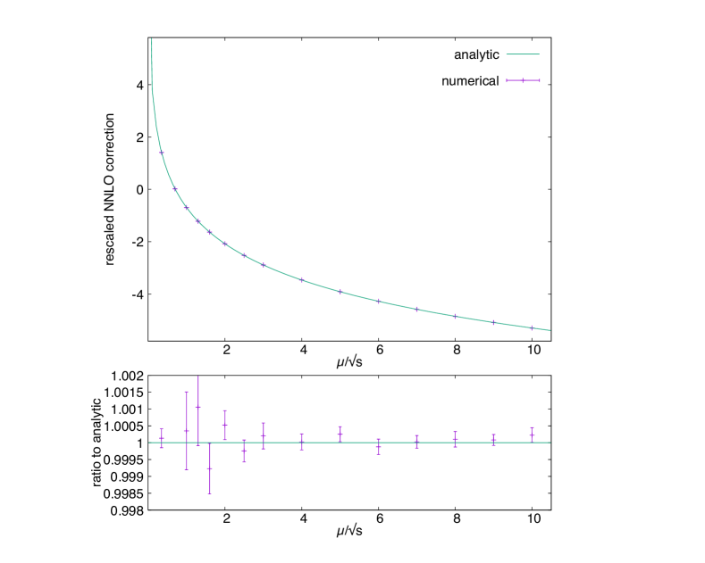
Figure 1: Rescaled NNLO correction as a function of the renormalisation scale.

5 Conclusions

In this work we have presented a new scheme to perform local analytic subtraction of infrared divergences up to NNLO in QCD. The method has for now been developed and applied to processes featuring only massless partons, and not involving coloured partons in the initial state, as a first significant step towards a general formulation. Our subtraction procedure is conceived with the aim of minimising complexity in the definition of the local IR counterterms, aiming for their complete analytic integration in the unresolved phase space, and working towards an optimal organisation of the numerical integration of the observable cross section.

Our local IR counterterms are defined through a unitary partition of the phase space into sectors, in such a way as to isolate in each sector a minimal number of phase-space singularities, associated with soft and collinear configurations of an identified set of partons (up to two at NLO, and up to four at NNLO). In each sector, the counterterms are built out of a collection of universal kernels, written in terms of kinematic invariants, which can be defined in terms of gauge-invariant operator matrix elements, as detailed in Magnea:2018ebr , or can be obtained as limits of radiative matrix elements in the dominant soft and collinear configurations. Overlapping singularities are fully taken into account by suitable compositions of such singular limits, with no need to resort to sector-decomposition techniques.

The sector functions that realise the phase-space partition are engineered in such a way as to satisfy fundamental relations that allow to achieve the main goals of the method. A number of sum rules, stemming from the definition of the sector functions, allow one to recombine various subsets of sectors, prior to performing counterterm integration, eventually yielding integrands that in all cases are solely made up by sums of elementary infrared and collinear kernels. Moreover, through factorisation relations, NNLO sector functions reproduce the complete structure of NLO sectors in all relevant single-unresolved limits, allowing to subtract, sector by sector in the NLO phase space, the singularities of the NNLO contributions featuring NLO kinematics.

The kinematic mappings necessary for phase-space factorisation, as well as the parametrisations of the radiation phase space over which the counterterms are integrated, are devised by maximally exploiting the freedom one has in their definition. They are not only chosen differently for different sectors, but also, importantly, for different counterterm contributions in the same sector. This allows us to employ parametrisations that are naturally adapted to the kinematic invariants that appear in each singular contribution, yielding simple integrands to be evaluated analytically.

In this article we have integrated all needed counterterms over the exact phase-space measures, without exploring the possibility of approximating the latter in the relevant soft and collinear limits. While this possibility would not have resulted in any analytic simplification in the cases considered here, this might instead be the case for general hadronic reactions (for example when including initial-state partons, or for a generalisation to the massive case). This possibility will be investigated in dedicated future studies, which are beyond the scope of the present paper.

At NLO, we have shown that the proposed subtraction method works in the general case of massless QCD final states, with the integrated counterterms reproducing analytically the full structure of virtual one-loop singularities. Moreover, as a test of the power of the method, we have shown that the NLO counterterm integration can be performed exactly to all orders in the dimensional regulator $\epsilon$, which bears witness to the extreme simplicity of the integrands involved.

At NNLO, we have deduced the structure of the subtraction scheme in full generality for massless QCD final states. All single-unresolved and mixed double-unresolved counterterms of double-real origin have been integrated analytically to all orders in $\epsilon$, as simply as in the NLO case, and the properties of sector functions have allowed us to show that these integrals correctly reproduce, sector by sector, the explicit $\epsilon$ poles and phase-space singularities of real-virtual contributions. We stress that this is a highly non-trivial test of the consistency of the scheme, and of the delicate organisation of different contributions to the cross section. As for double-unresolved counterterms, we have deduced their structure in general, and performed the relevant integrations in a proof-of-concept case, the $T_{R}C_{F}$ contribution to $e^{+}e^{-}\to q\bar{q}$ at NNLO, which has been detailed explicitly.

While in this paper we have concentrated on the general structure of our method, in particular concerning sector functions and phase-space mappings, and we have given only a simple example of implementation, we emphasize that we do not expect significant further technical difficulties for the extension of our algorithm to a general massless final states at NNLO: indeed, an important advantage of our method is that the required local counterterms are essentially combinations of the (re-mapped) NNLO splitting kernels. The corresponding integrals are therefore closely related to integrals known in the literature (see, for example Gehrmann-DeRidder:Thesis ; Gehrmann-DeRidder:2003pne ), and they are not expected to pose an obstacle for a general application of the method. The inclusion of initial state radiation is expected to require more work, in order to design and test appropriate sector functions and dedicated phase-space mappings, as well as implementing collinear factorization, but no new conceptual problems are expected to arise.

To summarize, this article represents a first step towards the formulation of a general, local, analytic, and minimal subtraction scheme, relevant for generic multi-particle hadronic processes at NNLO in QCD. To reach this goal, a number of important steps still need to be taken, including the analytic integration of the remaining double-unresolved counterterms for final-state processes, the generalisation to include initial-state massless partons, and the extension to the massive case, as well as the completion of an efficient computer code implementing the subtraction method in a fully differential framework. We believe however that the present work lays a solid foundation for these future developments.

Appendix A Commutation of soft and collinear limits at NLO

In this Appendix, as an example, we explicitly show the commutation of the soft and collinear limits ${\bf S}_{i}$ and ${\bf C}_{ij}$, and, in the process, deduce the form of the soft-collinear kernel ${\bf S}_{i}\,P_{ij}$ appearing in Eq. (20). The action of operators ${\bf S}_{i}$ and ${\bf C}_{ij}$ on ratios of elementary massless invariants $s_{ij}$ is given by

$${\bf S}_{i}\,\frac{s_{ia}}{s_{ib}} \neq 0\,,\qquad\quad\,\,\,{\bf S}_{i}\,\frac{s_{ia}}{s_{bc}}\,=\,0\,,\qquad\forall\,a,b,c\neq i\,,$$ (166)

$${\bf C}_{ij}\,\frac{s_{ij}}{s_{ab}} = 0\,,\qquad\quad{\bf C}_{ij}\,\frac{s_{ia}}{s_{ja}}\,=\,\mbox{independent of $a$}\,,\qquad\forall\,ab\notin\pi(ij)\,.$$ (167)

We start by verifying that the sequential action of the singular projectors on sector functions does not depend on their ordering. To this end note that

$${\bf S}_{i}\,\mathcal{W}_{ij}\,=\,\frac{1/w_{ij}}{\sum\limits_{l\neq i}1/w_{il}}\qquad \Longrightarrow \qquad{\bf C}_{ij}\,{\bf S}_{i}\,\mathcal{W}_{ij}\,=\,1\,,$$ (168)

$${\bf C}_{ij}\,\mathcal{W}_{ij}\,=\,\frac{e_{j}}{e_{i}+e_{j}}\qquad \Longrightarrow \qquad{\bf S}_{i}\,{\bf C}_{ij}\,\mathcal{W}_{ij}\,=\,1\,,$$ (169)

where in Eq. (168) we used the fact that only $l=j$ gives rise to a singular contribution $1/w_{il}$ in the collinear limit, while in Eq. (169) we have noted that $e_{i}\to 0$ in the soft limit.

Next, we consider the action of the composite projector ${\bf S}_{i}\,{\bf C}_{ij}$ on the physical real-radiation amplitude squared, where, without loss of generality, we drop all kinematic dependences in the real and Born-like matrix elements. Starting from Eq. (19) we find

$${\bf S}_{i}\,{\bf C}_{ij}\,R\,=\,\frac{\mathcal{N}_{1}}{s_{ij}}\,\Big{[}{\bf S}_{i}\,P_{ij}\,B+{\bf S}_{i}\,Q_{ij}^{\mu\nu}{B}_{\mu\nu}\Big{]}\,.$$ (170)

We now note that $Q_{ij}^{\mu\nu}$, defined in Eq. (29), is not singular in the soft limit for parton $i$, hence ${\bf S}_{i}\,Q_{ij}^{\mu\nu}=0$. The same happens for all terms in $P_{ij}$ which do not contain a denominator $1/x_{i}$. We now rewrite the remaining contributions in terms of Mandelstam invariants, using the definition of $x_{i}$ and $x_{j}$ in Eq. (26), with the result

$$P_{ij} = \delta_{f_{i}g}\,\delta_{f_{j}g}\,2C_{A}\,\frac{x_{j}}{x_{i}}+\delta_{f_{i}g}\,\delta_{f_{j}\{q,\bar{q}\}}\,C_{F}\,\frac{1+x_{j}^{2}}{x_{i}}+\,\ldots\,,$$ (171)

$$= \delta_{f_{i}g}\,\delta_{f_{j}g}\,2C_{A}\,\frac{s_{jr}}{s_{ir}}+\delta_{f_{i}g}\,\delta_{f_{j}\{q,\bar{q}\}}\,C_{F}\,\frac{1+\big{[}s_{jr}/\left(s_{ir}+s_{jr}\right)\big{]}^{2}}{s_{ir}/\left(s_{ir}+s_{jr}\right)}+\,\ldots\,,$$

where the ellipses denote terms that remain regular as parton $i$ becomes soft. Taking now the ${\bf S}_{i}$ limit according to Eq. (166), we get

$${\bf S}_{i}\,P_{ij} = \delta_{f_{i}g}\,\delta_{f_{j}g}\,2C_{A}\,\frac{s_{jr}}{s_{ir}}+\delta_{f_{i}g}\,\delta_{f_{j}\{q,\bar{q}\}}\,C_{F}\,\frac{2s_{jr}}{s_{ir}}$$ (172)

$$= \delta_{f_{i}g}\,\delta_{f_{j}g}\,2C_{A}\,\frac{x_{j}}{x_{i}}+\delta_{f_{i}g}\,\delta_{f_{j}\{q,\bar{q}\}}\,C_{F}\,\frac{2x_{j}}{x_{i}}\,,$$

which is Eq. (30). In particular, we note that the soft limit ${\bf S}_{i}$ does not correspond to taking $x_{i}\to 0$, rather to taking $s_{ir}\to 0$ (the two definitions differ by subleading soft terms). The soft-collinear limit is thus

$${\bf S}_{i}\,{\bf C}_{ij}\,R\,=\,B\,\,\frac{\mathcal{N}_{1}}{s_{ij}}\left(\delta_{f_{i}g}\,\delta_{f_{j}g}\,2C_{A}\,\frac{s_{jr}}{s_{ir}}+\delta_{f_{i}g}\,\delta_{f_{j}\{q,\bar{q}\}}\,C_{F}\,\frac{2s_{jr}}{s_{ir}}\right)\,.$$ (173)

We can now verify commutation by considering the two singular limits in reversed order. We find

$${\bf C}_{ij}\,{\bf S}_{i}\,R\,=\,-\,\mathcal{N}_{1}\,{\bf C}_{ij}\sum_{k\neq i\,,l\neq i}\!\mathcal{I}_{kl}^{(i)}\,{B}_{kl}\,.$$ (174)

Among all the terms in the double sum, only those with $k=j$ or $l=j$ are singular in the collinear limit, hence

$${\bf C}_{ij}\,{\bf S}_{i}\,R = -\,\mathcal{N}_{1}\,\frac{2}{s_{ij}}\,{\bf C}_{ij}\,\sum_{l\neq i}\frac{s_{jl}}{s_{il}}\,B_{jl}\,.$$ (175)

According to property (167), in the collinear limit ${\bf C}_{ij}$ the ratio $s_{jl}/s_{il}$ is independent of $l$: we can therefore set $l=r$ and get

$${\bf C}_{ij}\,{\bf S}_{i}\,R = -\,\mathcal{N}_{1}\,\delta_{f_{i}g}\,\frac{2}{s_{ij}}\,\frac{s_{jr}}{s_{ir}}\sum_{l\neq i}{B}_{jl}\,=\,\mathcal{N}_{1}\,\frac{2}{s_{ij}}\frac{s_{jr}}{s_{ir}}\,C_{f_{j}}B$$ (176)

$$= B\,\,\frac{\mathcal{N}_{1}}{s_{ij}}\left(\delta_{f_{i}g}\,\delta_{f_{j}g}\,2C_{A}\,\frac{s_{jr}}{s_{ir}}+\delta_{f_{i}g}\,\delta_{f_{j}\{q,\bar{q}\}}\,C_{F}\,\frac{2s_{jr}}{s_{ir}}\right)\,,$$

where in the last two steps we have used colour algebra, and the definition of the Casimir operator $C_{f_{j}}=C_{A}\delta_{f_{j}g}+C_{F}\delta_{f_{j}\{q\bar{q}\}}$. The equality of Eq. (176) and Eq. (173), together with relations (168) and (169), shows the desired commutation of limits in each sector $ij$.

Appendix B Soft and collinear limits of sector functions

In this Appendix we explore the properties of the NNLO sector functions defined in Eqs. (63) and (64), including their relation to the NLO-like functions defined in Eq. (67). We begin by establishing which limits, among ${\bf S}_{a}$, ${\bf C}_{ab}$, ${\bf S}_{ab}$, ${\bf C}_{abc}$, ${\bf C}_{abcd}$, ${\bf SC}_{abc}$, and ${\bf CS}_{abc}$, are non-vanishing in the three sector topologies $\mathcal{W}_{ijjk}$, $\mathcal{W}_{ijkj}$ and $\mathcal{W}_{ijkl}$. To this end, we start by analysing the behaviour of the sector-function denominator $\sigma$ (see Eq. (63)), in these limits. We find

$${\bf S}_{i}\,\sigma = \sum_{b\neq i}\sum_{c\neq i}\sum_{d\neq i,c}{\bf S}_{i}\,\sigma_{ibcd}\,=\,\sum_{b\neq i}\sigma_{ib}^{(\alpha\beta)}\sum_{c\neq i}\sum_{d\neq i,c}\sigma_{cd}\,,$$

$${\bf C}_{ij}\,\sigma = \sum_{c\neq i}\sum_{d\neq i,c}\sigma_{ijcd}+\sum_{c\neq j}\sum_{d\neq j,c}\sigma_{jicd}$$

$$= \left[\sigma_{ij}^{(\alpha\beta)}+\sigma_{ji}^{(\alpha\beta)}\right]\bigg{[}\sum_{c\neq i,j}\sigma_{c[ij]}+\sum_{d\neq i,j}\sigma_{[ij]d}+\sum_{c\neq i,j}\sum_{d\neq i,j,c}\sigma_{cd}\bigg{]}\,,$$

$${\bf S}_{ij}\,\sigma = \sum_{b\neq i}\sum_{d\neq i,j}\sigma_{ibjd}+\sum_{b\neq j}\sum_{d\neq j,i}\sigma_{jbid}\,,$$

$${\bf C}_{ijk}\,\sigma = \sigma_{ijjk}+\sigma_{ijkj}+\sigma_{ikkj}+\sigma_{ikjk}+\sigma_{jiik}+\sigma_{jiki}$$

$$+\,\sigma_{jkki}+\sigma_{jkik}+\sigma_{kiij}+\sigma_{kiji}+\sigma_{kjji}+\sigma_{kjij}\,,$$

$${\bf C}_{ijkl}\,\sigma = \sigma_{ijkl}+\sigma_{ijlk}+\sigma_{jikl}+\sigma_{jilk}+\sigma_{klij}+\sigma_{klji}+\sigma_{lkij}+\sigma_{lkji}\,,$$

$${\bf SC}_{ijk}\,\sigma = \sum_{b\neq i}\,{\bf S}_{i}\left(\sigma_{ibjk}+\sigma_{ibkj}\right)\,=\,\sum_{b\neq i}\sigma_{ib}^{(\alpha\beta)}\left(\sigma_{jk}+\sigma_{kj}\right)\,,$$

$${\bf CS}_{ijk}\,\sigma = \sum_{d\neq i,k}\sigma_{ijkd}+\sum_{d\neq j,k}\sigma_{jikd}\,=\,\sigma_{ij}^{(\alpha\beta)}\sum_{d\neq i,k}\sigma_{kd}\,+\,\sigma_{ji}^{(\alpha\beta)}\sum_{d\neq j,k}\sigma_{kd}\,,$$ (177)

where $[ij]$ denotes the parent parton of $i$ and $j$ and we have used the definition of the NLO-like sector functions in Eq. (67). Now we note that a singular limit $\bf L$ gives a non-zero result, when applied to the sector functions $\mathcal{W}_{abcd}$, only if the numerator of the latter, $\sigma_{abcd}$, appears as one of the addends of $\bf{L}\,\sigma$. Inspection of Eq. (177) then proves that the limits reported in Eq. (66) exhaust the surviving ones in each sector.

Next, we show that all of the limits in Eq. (66) commute when acting on $\sigma$. This is a crucial step for our method, since commutation of limits drastically reduces the number of independent configurations one needs to explore. Furthermore, one must note that, while commutation can be understood from physical considerations when limits are taken on squared matrix elements, sector functions are a crucial but artificial ingredient of our method, and commutation of limits is non-trivial in this case. We list below all relevant ordered limits, acting on the denominator function $\sigma$, beginning with those involving the single-soft limit ${\bf S}_{i}$.

$${\bf S}_{i}\,{\bf C}_{ij}\,\sigma\,=\,{\bf C}_{ij}\,{\bf S}_{i}\,\sigma = \sum_{c\neq i}\sum_{d\neq i,c}{\bf S}_{i}\,\sigma_{ijcd}\,=\,\sigma_{ij}^{(\alpha\beta)}\sum_{c\neq i}\sum_{d\neq i,c}\sigma_{cd}\,,$$

$${\bf S}_{i}\,{\bf S}_{ij}\,\sigma\,=\,{\bf S}_{ij}\,{\bf S}_{i}\,\sigma = \sum_{b\neq i}\sum_{d\neq i,j}{\bf S}_{i}\,\sigma_{ibjd}\,=\,\sum_{b\neq i}\sigma_{ib}^{(\alpha\beta)}\sum_{d\neq i,j}\sigma_{jd}\,,$$

$${\bf S}_{i}\,{\bf C}_{ijk}\,\sigma\,=\,{\bf C}_{ijk}\,{\bf S}_{i}\,\sigma = {\bf S}_{i}\left(\sigma_{ijjk}+\sigma_{ijkj}+\sigma_{ikkj}+\sigma_{ikjk}\right)\,=\,\left[\sigma_{ij}^{(\alpha\beta)}+\sigma_{ik}^{(\alpha\beta)}\right]\big{(}\sigma_{jk}+\sigma_{kj}\big{)}\,,$$

$${\bf S}_{i}\,{\bf C}_{ijkl}\,\sigma\,=\,{\bf C}_{ijkl}\,{\bf S}_{i}\,\sigma = \sigma_{ijkl}+\sigma_{ijlk}\,=\,\sigma_{ij}^{(\alpha\beta)}\left(\sigma_{kl}+\sigma_{lk}\right)\,,$$

$${\bf S}_{i}\,{\bf SC}_{ijk}\,\sigma\,=\,{\bf SC}_{ijk}\,{\bf S}_{i}\,\sigma = {\bf SC}_{ijk}\,\sigma\,=\,\sum_{b\neq i}{\bf S}_{i}\left(\sigma_{ibjk}+\sigma_{ibkj}\right)\,=\,\sum_{b\neq i}\sigma_{ib}^{(\alpha\beta)}\left(\sigma_{jk}+\sigma_{kj}\right)\,,$$

$${\bf S}_{i}\,{\bf CS}_{ijk}\,\sigma\,=\,{\bf CS}_{ijk}\,{\bf S}_{i}\,\sigma = \sum_{d\neq i,k}\sigma_{ijkd}\,=\,\sigma_{ij}^{(\alpha\beta)}\sum_{d\neq i,k}\sigma_{kd}\,.$$ (178)

Next, we list ordered limits involving the single-collinear limit ${\bf C}_{ij}$, and not considered above.

$${\bf C}_{ij}\,{\bf S}_{ij}\,\sigma\,=\,{\bf S}_{ij}\,{\bf C}_{ij}\,\sigma = \sum_{d\neq i,j}\left(\sigma_{ijjd}+\sigma_{jiid}\right)\,=\,\left[\sigma_{ij}^{(\alpha\beta)}+\sigma_{ji}^{(\alpha\beta)}\right]\sum_{d\neq i,j}\sigma_{[ij]d}\,,$$

$${\bf C}_{ij}\,{\bf S}_{ik}\,\sigma\,=\,{\bf S}_{ik}\,{\bf C}_{ij}\,\sigma = \sum_{d\neq i,k}\sigma_{ijkd}\,=\,\sigma_{ij}^{(\alpha\beta)}\bigg{[}\sigma_{k[ij]}+\sum_{d\neq i,j,k}\sigma_{kd}\bigg{]}\,,$$

$${\bf C}_{ij}\,{\bf C}_{ijk}\,\sigma\,=\,{\bf C}_{ijk}\,{\bf C}_{ij}\,\sigma = \sigma_{ijjk}+\sigma_{ijkj}+\sigma_{jiik}+\sigma_{jiki}\,=\,\left[\sigma_{ij}^{(\alpha\beta)}+\sigma_{ji}^{(\alpha\beta)}\right]\left(\sigma_{[ij]k}+\sigma_{k[ij]}\right)\,,$$

$${\bf C}_{ij}\,{\bf C}_{ijkl}\,\sigma\,=\,{\bf C}_{ijkl}\,{\bf C}_{ij}\,\sigma = \sigma_{ijkl}+\sigma_{ijlk}+\sigma_{jikl}+\sigma_{jilk}\,=\,\left[\sigma_{ij}^{(\alpha\beta)}+\sigma_{ji}^{(\alpha\beta)}\right]\big{(}\sigma_{kl}+\sigma_{lk}\big{)}\,,$$

$${\bf C}_{ij}\,{\bf SC}_{ijk}\,\sigma\,=\,{\bf SC}_{ijk}\,{\bf C}_{ij}\,\sigma = {\bf S}_{i}\left(\sigma_{ijjk}+\sigma_{ijkj}\right)\,=\,\sigma_{ij}^{(\alpha\beta)}\big{(}\sigma_{jk}+\sigma_{kj}\big{)}\,,$$ (179)

$${\bf C}_{ij}\,{\bf SC}_{ikl}\,\sigma\,=\,{\bf SC}_{ikl}\,{\bf C}_{ij}\,\sigma = \sigma_{ijkl}+\sigma_{ijlk}\,=\,\sigma_{ij}^{(\alpha\beta)}\big{(}\sigma_{kl}+\sigma_{lk}\big{)}\,,$$

$${\bf C}_{ij}\,{\bf CS}_{ijk}\,\sigma\,=\,{\bf CS}_{ijk}\,{\bf C}_{ij}\,\sigma = {\bf CS}_{ijk}\,\sigma\,=\,\!\sum_{d\neq i,k}\!\sigma_{ijkd}+\!\sum_{d\neq j,k}\!\sigma_{jikd}\,=\,\!\sigma_{ij}^{(\alpha\beta)}\!\!\sum_{d\neq i,k}\!\sigma_{kd}+\sigma_{ji}^{(\alpha\beta)}\!\!\sum_{d\neq j,k}\!\sigma_{kd}\,.$$

Moving on to ordered limits involving the double-soft limit ${\bf S}_{ab}$, and not considered above, we find

$${\bf S}_{ij}\,{\bf C}_{ijk}\,\sigma\,=\,{\bf C}_{ijk}\,{\bf S}_{ij}\,\sigma = \sigma_{ijjk}+\sigma_{jiik}+\sigma_{ikjk}+\sigma_{jkik}\,,$$

$${\bf S}_{ik}\,{\bf C}_{ijkl}\,\sigma\,=\,{\bf C}_{ijkl}\,{\bf S}_{ik}\,\sigma = \sigma_{ijkl}+\sigma_{klij}\,=\,\sigma_{ij}^{(\alpha\beta)}\sigma_{kl}+\sigma_{kl}^{(\alpha\beta)}\sigma_{ij}\,,$$

$${\bf S}_{ij}\,{\bf SC}_{ijk}\,\sigma\,=\,{\bf SC}_{ijk}\,{\bf S}_{ij}\,\sigma = \sum_{b\neq i}\,{\bf S}_{i}\,\sigma_{ibjk}\,=\,\sum_{b\neq i}\sigma_{ib}^{(\alpha\beta)}\,\sigma_{jk}\,,$$ (180)

$${\bf S}_{ik}\,{\bf CS}_{ijk}\,\sigma\,=\,{\bf CS}_{ijk}\,{\bf S}_{ik}\,\sigma = {\bf S}_{i}\,{\bf CS}_{ijk}\,\sigma\,=\,{\bf CS}_{ijk}\,{\bf S}_{i}\,\sigma\,=\,\sum_{d\neq i,k}\!\sigma_{ijkd}\,=\,\sigma_{ij}^{(\alpha\beta)}\sum_{d\neq i,k}\!\sigma_{kd}\,.$$

Coming to double-collinear limits of type ${\bf C}_{ijk}$ and ${\bf C}_{ijkl}$, we get

$${\bf C}_{ijk}\,{\bf SC}_{ijk}\,\sigma\,=\,{\bf SC}_{ijk}\,{\bf C}_{ijk}\,\sigma = {\bf S}_{i}\,{\bf C}_{ijk}\,\sigma\,=\,{\bf C}_{ijk}\,{\bf S}_{i}\,\sigma$$

$$= {\bf S}_{i}\big{(}\sigma_{ijjk}+\sigma_{ijkj}+\sigma_{ikjk}+\sigma_{ikkj}\big{)}\,=\,\left[\sigma_{ij}^{(\alpha\beta)}+\sigma_{ik}^{(\alpha\beta)}\right]\big{(}\sigma_{jk}+\sigma_{kj}\big{)},$$

$${\bf C}_{ijkl}\,{\bf SC}_{ikl}\,\sigma\,=\,{\bf SC}_{ikl}\,{\bf C}_{ijkl}\,\sigma = {\bf S}_{i}\,{\bf C}_{ijkl}\,\sigma\,=\,{\bf C}_{ijkl}\,{\bf S}_{i}\,\sigma\,=\,\sigma_{ijkl}+\sigma_{ijlk}\,=\,\sigma_{ij}^{(\alpha\beta)}\big{(}\sigma_{kl}+\sigma_{lk}\big{)}\,,$$

$${\bf C}_{ijk}\,{\bf CS}_{ijk}\,\sigma\,=\,{\bf CS}_{ijk}\,{\bf C}_{ijk}\,\sigma = \sigma_{ijkj}+\sigma_{jiki}\,,$$

$${\bf C}_{ijkl}\,{\bf CS}_{ijk}\,\sigma\,=\,{\bf CS}_{ijk}\,{\bf C}_{ijkl}\,\sigma = \sigma_{ijkl}+\sigma_{jikl}\,.$$ (181)

Finally, the mixed soft-collinear limits ${\bf SC}_{ijk}$ and ${\bf CS}_{ijk}$ satisfy

$${\bf SC}_{ijk}\,{\bf CS}_{ijk}\,\sigma\,=\,{\bf CS}_{ijk}\,{\bf SC}_{ijk}\,\sigma = \sigma_{ijkj}\,,$$

$${\bf SC}_{ikl}\,{\bf CS}_{ijk}\,\sigma\,=\,{\bf CS}_{ijk}\,{\bf SC}_{ikl}\,\sigma = \sigma_{ijkl}\,.$$ (182)

The relations in Eqs. (178)-(182), where the limits are applied to the sector-function denominator $\sigma$, are sufficient to prove that all non-vanishing limits in the different topologies commute when acting on the sector functions. The same commutation relations hold when applied to the physical double-real matrix elements, as can be proved analogously to what was done in Appendix A.

The next step in our analysis is to prove that the compositions of the limits given in Eq. (66) exhaust all single- and double-unresolved configurations in each sector. In other words, there are no leftover singular phase-space regions after all combinations of limits in Eq. (66) have been applied. We start by denoting with ${\bf L}_{i}$ a generic set of soft and collinear limits, corresponding to configurations where some physical quantities $\lambda_{i}$, which could be collections of energies, or angles, or similar, approach zero. Compositions of two (or more) such limits can be either ‘uniform’ or ‘ordered’, with the two cases being defined as

$$[{\bf L}_{j}{\bf L}_{i}]\,=\,[{\bf L}_{i}{\bf L}_{j}] : \left\{\begin{array}[]{l}\lambda_{i}\,,\,\lambda_{j}\,\to\,0\\ \lambda_{i}/\lambda_{j}\,\to\,\mbox{const.}\end{array}\right.\quad\Longleftrightarrow\quad\mbox{uniform composition of ${\bf L}_{i}$ and ${\bf L}_{j}$ ;}$$ (185)

$${\bf L}_{j}{\bf L}_{i} : \left\{\begin{array}[]{l}\lambda_{i}\,,\,\lambda_{j}\,\to\,0\\ \lambda_{i}/\lambda_{j}\,\to\,0\end{array}\right.\quad\Longleftrightarrow\quad\mbox{ordered composition of ${\bf L}_{i}$ (first) and ${\bf L}_{j}$ .}$$ (188)

All single- and double-unresolved configurations in each sector can then be systematically generated by combining in all possible ways the single-soft and single-collinear limits selected by the sector functions, namely ${\bf S}_{a}$, ${\bf S}_{c}$, ${\bf C}_{ab}$, and ${\bf C}_{cd}$ in sector $\mathcal{W}_{abcd}$.

Owing to the prescription $\alpha>\beta>1$ in Eq. (64), the action on $\sigma$ of a uniform composition involving soft and collinear limits is equivalent to the corresponding ordered composition where the soft limits act first:

$${\bf L}^{\prime}\,[{\bf L}_{\rm c}\,{\bf L}_{{\rm\,s}}]\,{\bf L}\,\sigma\,=\,{\bf L}^{\prime}\,[{\bf L}_{\rm c}][{\bf L}_{{\rm\,s}}]\,{\bf L}\,\sigma\,,$$ (189)

where ${\bf L}_{{\rm\,s}}$ (${\bf L}_{\rm c}$) are collections of soft (collinear) limits, while ${\bf L}$, and ${\bf L}^{\prime}$ are generic combinations of limits. The remaining uniform compositions involve either a pair of collinear or a pair of soft limits, which can be directly identified with the limits given in Eq. (66):

$$[{\bf S}_{i}\,{\bf S}_{j}]\,=\,{\bf S}_{ij}\,,\qquad[{\bf C}_{ij}\,{\bf C}_{jk}]\,=\,{\bf C}_{ijk}\,,\qquad[{\bf C}_{ij}\,{\bf C}_{kl}]\,=\,{\bf C}_{ijkl}\,.$$ (190)

We conclude that all possible single- and double-unresolved singular configurations can be obtained as ordered compositions without repetition⁷ of the limits

• ${\bf S}_{i}$,   ${\bf S}_{j}$,   ${\bf C}_{ij}$,   ${\bf C}_{jk}$,   ${\bf S}_{ij}$,   and   ${\bf C}_{ijk}$   for topology $\mathcal{W}_{ijjk}$ ;
  

• ${\bf S}_{i}$,   ${\bf S}_{k}$,   ${\bf C}_{ij}$,   ${\bf C}_{jk}$,   ${\bf S}_{ik}$,   and   ${\bf C}_{ijk}$   for topology $\mathcal{W}_{ijkj}$ ;
  

• ${\bf S}_{i}$,   ${\bf S}_{k}$,   ${\bf C}_{ij}$,   ${\bf C}_{kl}$,   ${\bf S}_{ik}$,   and   ${\bf C}_{ijkl}$   for topology $\mathcal{W}_{ijkl}$ .

To conclude, we reduce this list of limits, topology by topology, to that given in Eq. (66).

• Topology $\mathcal{W}_{ijjk}$
  According to Eqs. (178)-(182), the ${\bf S}_{j}$ limit commutes with all other limits in the list except ${\bf S}_{i}$. Therefore, when appearing in a generic composition of limits, it can be moved to the right until it encounters ${\bf S}_{i}$. At this point one can use

  $${\bf L}^{\prime}\,{\bf S}_{j}\,{\bf S}_{i}\,{\bf L}\,\mathcal{W}_{ijjk}\,=\,{\bf L}^{\prime}\,{\bf S}_{ij}\,{\bf S}_{i}\,{\bf L}\,\mathcal{W}_{ijjk}\,,$$ (191)

  valid for generic limits ${\bf L}$ and ${\bf L}^{\prime}$, to remove ${\bf S}_{j}$. If ${\bf S}_{i}$ is not present at the right of ${\bf S}_{j}$, the latter can be moved to the rightmost position, where it vanishes:

  $${\bf L}\,{\bf S}_{j}\,\mathcal{W}_{ijjk}\,=\,0\,.$$ (192)

  Since the action of ${\bf S}_{j}$ either gives zero or can be replaced by that of ${\bf S}_{ij}$, ${\bf S}_{j}$ can be simply removed from the list.

  Considering now ${\bf C}_{jk}$, we note that it commutes with ${\bf C}_{ijk}$ and with ${\bf S}_{ij}$, and it satisfies

  $${\bf L}^{\prime}\,{\bf C}_{jk}\,{\bf S}_{i}\,{\bf L}\,\mathcal{W}_{ijjk} = {\bf L}^{\prime}\,{\bf SC}_{ijk}\,{\bf L}\,\mathcal{W}_{ijjk}\,,$$

  $${\bf L}^{\prime}\,{\bf C}_{jk}\,{\bf C}_{ij}\,{\bf L}\,\mathcal{W}_{ijjk} = {\bf L}^{\prime}\,{\bf C}_{ijk}\,{\bf C}_{ij}\,{\bf L}\,\mathcal{W}_{ijjk}\,,$$

  $${\bf L}^{\prime}\,{\bf C}_{jk}\,\mathcal{W}_{ijjk} = 0\,,$$ (193)

  so that ${\bf C}_{jk}$ can either be moved to the rightmost position, where it gives zero, or replaced by ${\bf C}_{ijk}$ or ${\bf SC}_{ijk}$. Consequently, one can remove ${\bf C}_{jk}$ from the list of limits, and add ${\bf SC}_{ijk}$ in its stead. The list of singular limits is thus reduced to the first line of Eq. (66),

  $$\mathcal{W}_{ijjk} : \,\,{\bf S}_{i}\,,\,{\bf C}_{ij}\,,\,{\bf S}_{ij}\,,\,{\bf C}_{ijk}\,,\,{\bf SC}_{ijk}\,.$$ (194)

• Topology $\mathcal{W}_{ijkj}$
  Besides commuting with ${\bf C}_{jk}$, ${\bf S}_{ik}$, and ${\bf C}_{ijk}$, the single-soft limit ${\bf S}_{k}$ satisfies

  $${\bf L}^{\prime}\,{\bf S}_{k}\,{\bf S}_{i}\,{\bf L}\,\mathcal{W}_{ijkj} = {\bf L}^{\prime}\,{\bf S}_{ik}\,{\bf S}_{i}\,{\bf L}\,\mathcal{W}_{ijkj}\,,$$

  $${\bf L}^{\prime}\,{\bf S}_{k}\,{\bf C}_{ij}\,{\bf L}\,\mathcal{W}_{ijkj} = {\bf L}^{\prime}\,{\bf CS}_{ijk}\,{\bf L}\,\mathcal{W}_{ijkj}\,,$$

  $${\bf L}^{\prime}\,{\bf S}_{k}\,\mathcal{W}_{ijkj} = 0\,.$$ (195)

  Since ${\bf S}_{k}$ can be either moved to the rightmost position, where it gives zero, or replaced by ${\bf S}_{ik}$ or ${\bf CS}_{ijk}$, one can remove it from the list of contributing limits. A similar statement holds for ${\bf C}_{jk}$, which commutes with ${\bf S}_{ik}$, and ${\bf C}_{ijk}$, and satisfies

  $${\bf L}^{\prime}\,{\bf C}_{jk}\,{\bf S}_{i}\,{\bf L}\,\mathcal{W}_{ijkj} = {\bf L}^{\prime}\,{\bf SC}_{ijk}\,{\bf L}\,\mathcal{W}_{ijkj}\,,$$

  $${\bf L}^{\prime}\,{\bf C}_{jk}\,{\bf C}_{ij}\,{\bf L}\,\mathcal{W}_{ijkj} = {\bf L}^{\prime}\,{\bf C}_{ijk}\,{\bf C}_{ij}\,{\bf L}\,\mathcal{W}_{ijkj}\,,$$

  $${\bf L}^{\prime}\,{\bf C}_{jk}\,{\bf CS}_{ijk}\,{\bf L}\,\mathcal{W}_{ijkj} = {\bf L}^{\prime}\,{\bf C}_{ijk}\,{\bf CS}_{ijk}\,{\bf L}\,\mathcal{W}_{ijkj}\,,$$

  $${\bf L}^{\prime}\,{\bf C}_{jk}\,\mathcal{W}_{ijkj} = 0\,.$$ (196)

  As a consequence, ${\bf C}_{jk}$ can either be moved to the rightmost position, where it gives zero, or replaced by ${\bf C}_{ijk}$ or ${\bf SC}_{ijk}$. The list of singular limits in sector $\mathcal{W}_{ijkj}$ can thus be reduced to the second line of Eq. (66),

  $$\mathcal{W}_{ijkj} : \,\,{\bf S}_{i}\,,\,{\bf C}_{ij}\,,\,{\bf S}_{ik}\,,\,{\bf C}_{ijk}\,,\,{\bf SC}_{ijk}\,,\,{\bf CS}_{ijk}\,.$$ (197)

• Topology $\mathcal{W}_{ijkl}$
  The discussion of the ${\bf S}_{k}$ and ${\bf C}_{kl}$ limits holds unchanged with respect to the one relevant for ${\bf S}_{k}$ and ${\bf C}_{kj}$ in topology $\mathcal{W}_{ijkj}$. These limits can either be moved to the rightmost position, where they yield zero, or be replaced by limits that are already present in the list, (${\bf S}_{ik}$ or ${\bf CS}_{ijk}$ in the case of ${\bf S}_{k}$, ${\bf C}_{ijkl}$ or ${\bf SC}_{ikl}$ in the case of ${\bf C}_{kl}$). The final list of contributing limits thus coincides with the third line of Eq. (66),

  $$\mathcal{W}_{ijkl} : \,\,{\bf S}_{i}\,,\,{\bf C}_{ij}\,,\,{\bf S}_{ik}\,,\,{\bf C}_{ijkl}\,,\,{\bf SC}_{ikl}\,,\,{\bf CS}_{ijk}\,.$$ (198)

Appendix C Composite IR limits of the double-real matrix element

In this Appendix we list the composite soft and collinear limits of the double real-radiation squared matrix element needed for the evaluation of the double-unresolved counterterm $\overline{K}^{\,(\mathbf{2})}+\overline{K}^{\,(\mathbf{12})}$ in Eq. (110), including the detailed dependence on the remapped phase-space variables described in Section 3.5. The remappings described in the following apply also to the corresponding sector functions $\overline{\mathcal{W}}_{ab}$ in Eq. (110). First, we consider composing a double-collinear limit and a collinear limit. We find

$$\overline{\bf C}_{ij}\,\overline{\bf C}_{ijk}RR = \mathcal{N}_{1}\,\frac{P_{ij}^{\mu\nu}\left(s_{ir},s_{jr}\right)}{s_{ij}}\,\,\overline{\bf C}_{jk}\,R_{\mu\nu}\!\left(\{\bar{k}\}^{(ijr)}\right)$$

$$= \frac{\mathcal{N}_{1}^{2}}{s_{ij}\bar{s}_{jk}^{(ijr)}}\,\Bigg{\{}\bigg{[}\left(P_{ij}+Q_{ij}\right)\left(\overline{P}_{jk}^{(ijr)}+\overline{Q}_{jk}^{(ijr)}\right)-\frac{d-2}{2}\,C_{F}\,Q_{ij}\,\delta_{f_{k}\{q,\bar{q}\}}\,x_{j}^{\prime}$$

$$\qquad\qquad-\,\frac{d-2}{2}\,Q_{ij}\,C_{f_{k}}\,\frac{x_{k}^{\prime}}{x_{j}^{\prime}}\,\frac{(2\tilde{k}\cdot\tilde{k}^{\prime})^{2}}{\tilde{k}^{2}\,\tilde{k}^{\prime 2}}\bigg{]}B\!\left(\{\bar{k}\}^{(ijr,jkr)}\right)$$

$$\qquad\qquad+\,(d-2)\bigg{[}\Big{(}\left(P_{ij}+Q_{ij}\right)\,\overline{Q}_{jk}^{(ijr)}+Q_{ij}\,C_{A}\,\delta_{f_{k}g}\left(2x_{j}^{\prime}x_{k}^{\prime}\right)\Big{)}\frac{\tilde{k}^{\prime\mu}\tilde{k}^{\prime\nu}}{\tilde{k}^{\prime 2}}$$

$$\qquad\qquad\qquad\qquad\,\,+\,Q_{ij}\,C_{A}\,\delta_{f_{k}g}\,\frac{2x_{j}^{\prime}}{x_{k}^{\prime}}\,\frac{\tilde{k}^{\mu}\tilde{k}^{\nu}}{\tilde{k}^{2}}\bigg{]}B_{\mu\nu}\!\left(\{\bar{k}\}^{(ijr,jkr)}\right)\Bigg{\}}\,,$$

where $r\neq i,j,k$, and we introduced the shorthand notations

$$\overline{P}_{jk}^{(ijr)}\,=\,P_{jk}\left(\bar{s}_{jr}^{(ijr)},\bar{s}_{kr}^{(ijr)}\right)\,,\qquad\overline{Q}_{jk}^{(ijr)}\,=\,Q_{jk}\left(\bar{s}_{jr}^{(ijr)},\bar{s}_{kr}^{(ijr)}\right)\,.$$ (200)

The primed variables in Eq. (C) are defined in analogy to Eq. (26), as

$$\tilde{k}^{\prime} = x_{k}^{\prime}\,\bar{k}_{j}^{(ijr)}-x_{j}^{\prime}\,\bar{k}_{k}^{(ijr)}-\left(1-2x_{j}^{\prime}\right)\frac{\bar{s}_{jk}^{(ijr)}}{\bar{s}_{jr}^{(ijr)}+\bar{s}_{kr}^{(ijr)}}\,\bar{k}_{r}^{(ijr)}\,,$$ (202)

$$x_{j}^{\prime}\,=\,\frac{\bar{s}_{jr}^{(ijr)}}{\bar{s}_{jr}^{(ijr)}+\bar{s}_{kr}^{(ijr)}}\,,\qquad x_{k}^{\prime}\,=\,\frac{\bar{s}_{kr}^{(ijr)}}{\bar{s}_{jr}^{(ijr)}+\bar{s}_{kr}^{(ijr)}}\,.$$

Acting with further soft limits leads to

$$\overline{\bf C}_{ij}\,\overline{\bf S}_{ij}\,\overline{\bf C}_{ijk}RR = \mathcal{N}_{1}\,\frac{P_{ij}^{\mu\nu}\left(s_{ir},s_{jr}\right)}{s_{ij}}\,\,\overline{\bf S}_{j}\,\overline{\bf C}_{jk}\,R_{\mu\nu}\!\left(\{\bar{k}\}^{(ijr)}\right)$$

$$= \frac{\mathcal{N}_{1}^{\,2}}{s_{ij}}\,2\,C_{f_{k}}\,\frac{\bar{s}_{kr}^{(ijr)}}{\bar{s}_{jk}^{(ijr)}\bar{s}_{jr}^{(ijr)}}(\delta_{f_{i}g}\delta_{f_{j}g}+\delta_{\{f_{i}f_{j}\}\{q\bar{q}\}})$$

$$\,\times\,\bigg{[}P_{ij}+Q_{ij}\left(1-\frac{d-2}{4}\,\frac{(2\tilde{k}\cdot\tilde{k}^{\prime})^{2}}{\tilde{k}^{2}\,\tilde{k}^{\prime 2}}\right)\bigg{]}\!B\!\left(\{\bar{k}\}^{(ijr,jkr)}\right)\,,$$

$$\overline{\bf S}_{i}\,\overline{\bf C}_{ij}\,\overline{\bf C}_{ijk}RR = 2\,\mathcal{N}_{1}\,C_{f_{j}}\,\mathcal{I}_{jr}^{(i)}\,\overline{\bf C}_{jk}\,R\!\left(\!\{\bar{k}\}^{(ijr)}\!\right)$$

$$= 2\,\mathcal{N}_{1}^{\,2}\,C_{f_{j}}\,\mathcal{I}_{jr}^{(i)}\,\frac{P_{jk}^{\mu\nu}\left(\bar{s}_{jr}^{(ijr)},\bar{s}_{kr}^{(ijr)}\right)}{\bar{s}_{jk}^{(ijr)}}\,B_{\mu\nu}\!\left(\!\{\bar{k}\}^{(ijr,jkr)}\!\right)\,,$$

$$\overline{\bf S}_{i}\,\overline{\bf C}_{ij}\,\overline{\bf S}_{ij}\,\overline{\bf C}_{ijk}RR = 2\,\mathcal{N}_{1}\,C_{f_{j}}\,\mathcal{I}_{jr}^{(i)}\,\overline{\bf S}_{j}\,\overline{\bf C}_{jk}\,R\!\left(\!\{\bar{k}\}^{(ijr)}\!\right)$$

$$= 4\,\mathcal{N}_{1}^{\,2}\,\delta_{f_{j}g}\,C_{f_{j}}\,C_{f_{k}}\,\mathcal{I}_{jr}^{(i)}\,\frac{\bar{s}_{kr}^{(ijr)}}{\bar{s}_{jk}^{(ijr)}\bar{s}_{jr}^{(ijr)}}\,B\!\left(\!\{\bar{k}\}^{(ijr,jkr)}\!\right)\,,$$

where the same $r\neq i,j,k$ should be chosen for all permutations of $ijk$. Composition of a double-soft limit and a collinear limit (on the same pair of particles) yields

$$\overline{\bf C}_{ij}\,\overline{\bf S}_{ij}RR = \mathcal{N}_{1}\,\frac{P_{ij}^{\mu\nu}\left(s_{ir},s_{jr}\right)}{s_{ij}}\,\overline{\bf S}_{j}\,R_{\mu\nu}\!\left(\!\{\bar{k}\}^{(ijr)}\!\right)=\frac{\mathcal{N}_{1}^{\,2}}{2}\,\sum_{\begin{subarray}{c}c\neq i,j\\ d\neq i,j,c\end{subarray}}\!\mathcal{J}_{cd}^{(ij)}{B}_{cd}\Big{(}\!\{\bar{k}\}^{(ijr,jcd)}\!\Big{)}\,,$$ (206)

where the same $r\neq i,j$ should be chosen for all permutations of $ijk$ (recall that the index $k$ appears in the sector function associated with these contributions in Eq. (110)), and we have defined the quantities

$$\mathcal{J}_{cd}^{(ij)} = -\left[\delta_{f_{i}g}\delta_{f_{j}g}\,2\,C_{A}\left(\frac{x_{i}}{x_{j}}+\frac{x_{j}}{x_{i}}\right)+\delta_{\{f_{i}f_{j}\}\{q\bar{q}\}}\,T_{R}\right]\frac{2\,\bar{s}_{cd}^{(ijr)}}{s_{ij}\,\bar{s}_{jc}^{(ijr)}\bar{s}_{jd}^{(ijr)}}\,$$ (207)

$$\qquad\qquad\quad-\,(d\!-\!2)\,\frac{Q_{ij}\left(s_{ir},s_{jr}\right)}{2\,\tilde{k}^{2}\,s_{ij}}\,\Bigg{[}\frac{2\tilde{k}\cdot\bar{k}_{c}^{(ijr)}}{\bar{s}_{jc}^{(ijr)}}-\frac{2\tilde{k}\cdot\bar{k}_{d}^{(ijr)}}{\bar{s}_{jd}^{(ijr)}}\Bigg{]}^{2}\,.$$

Further applying the soft limit $\overline{\bf S}_{i}$ leads to

$$\overline{\bf S}_{i}\,\overline{\bf C}_{ij}\,\overline{\bf S}_{ij}RR = 2\,\mathcal{N}_{1}\,C_{f_{j}}\,\mathcal{I}_{jr}^{(i)}\,\overline{\bf S}_{j}\,R\!\left(\!\{\bar{k}\}^{(ijr)}\!\right)$$

$$= -\,2\,\mathcal{N}_{1}^{\,2}\,\delta_{f_{j}g}\,C_{f_{j}}\,\mathcal{I}_{jr}^{(i)}\,\sum_{\begin{subarray}{c}c\neq i,j\\ d\neq i,j\end{subarray}}\frac{\bar{s}_{cd}^{(ijr)}}{\bar{s}_{jc}^{(ijr)}\bar{s}_{jd}^{(ijr)}}\,B_{cd}\!\left(\!\{\bar{k}\}^{(ijr,jcd)}\!\right)\,.$$

As in Eq. (206), the same $r\neq i,j$ should be chosen for all permutations of $ijk$. Next, we consider the composition of the double-collinear limit $\overline{\bf C}_{ijkl}$ with a soft limit. We get

$$\overline{\bf S}_{i}\,\overline{\bf C}_{ijkl}RR = 2\,\mathcal{N}_{1}\,C_{f_{j}}\,\mathcal{I}_{jl}^{(i)}\,\overline{\bf C}_{kl}\,R\Big{(}\!\{\bar{k}\}^{(ijl)}\!\Big{)}$$

$$= 2\,\mathcal{N}_{1}^{\,2}\,C_{f_{j}}\mathcal{I}_{jl}^{(i)}\,\frac{P^{\mu\nu}_{kl}\left(\bar{s}_{kr}^{(ijl)},\bar{s}_{lr}^{(ijl)}\right)}{\bar{s}_{kl}^{(ijl)}}\,{B}_{\mu\nu}\Big{(}\!\{\bar{k}\}^{(ijl,klr)}\!\Big{)}\,,$$

where the same $r\neq i,k,l$ should be chose for all permutations in $\pi\left(\pi(ij)\pi(kl)\right)$. Acting with a further double soft limit $\overline{\bf S}_{ik}$ leads to

$$\overline{\bf S}_{i}\,\overline{\bf S}_{ik}\,\overline{\bf C}_{ijkl}RR = 4\,\mathcal{N}_{1}^{\,2}\,\delta_{{f_{k}}g}\,C_{f_{j}}\,C_{f_{l}}\,\mathcal{I}_{jl}^{(i)}\,\frac{\bar{s}_{lr}^{(ijl)}}{\bar{s}_{kl}^{(ijl)}\bar{s}_{kr}^{(ijl)}}\,{B}\Big{(}\!\{\bar{k}\}^{(ijl,klr)}\!\Big{)}$$

$$+\,2\,\mathcal{N}_{1}^{\,2}\,\delta_{{f_{k}}g}\,C_{f_{l}}\,\mathcal{I}_{jl}^{(i)}\,\left[\frac{\bar{s}_{lr}^{(ijl)}}{\bar{s}_{kl}^{(ijl)}\bar{s}_{kr}^{(ijl)}}\,{B}_{jl}\Big{(}\!\{\bar{k}\}^{(ijl,klr)}\!\Big{)}\,-\,\frac{\bar{s}_{lr}^{(ilj)}}{\bar{s}_{kl}^{(ilj)}\bar{s}_{kr}^{(ilj)}}\,{B}_{lj}\Big{(}\!\{\bar{k}\}^{(ilj,klr)}\!\Big{)}\right]\,,$$

where the same $r\neq i,k,l$ should be chosen for all permutations in $\pi(\pi(ij)\,\pi(kl))$.

Taking successively a double-soft limit and a single-soft limit, we get

$$\overline{\bf S}_{i}\,\overline{\bf S}_{ij}RR = -\,\mathcal{N}_{1}\sum_{c\neq i\,d\neq i}\mathcal{I}_{cd}^{(i)}\,\,\overline{\bf S}_{j}\,R_{cd}\Big{(}\!\{\bar{k}\}^{(icd)}\!\Big{)}$$

$$= \frac{\mathcal{N}_{1}^{2}}{2}\!\sum_{\begin{subarray}{c}c\neq i,j\\ d\neq i,j,c\end{subarray}}\!\Bigg{[}\sum_{\begin{subarray}{c}e\neq i,j,c,d\\ f\neq i,j,c,d\end{subarray}}\!\mathcal{I}_{cd}^{(i)}\,\delta_{f_{j}g}\,\frac{\bar{s}_{ef}^{(icd)}}{\bar{s}_{ej}^{(icd)}\bar{s}_{fj}^{(icd)}}{B}_{cdef}\Big{(}\!\{\bar{k}\}^{(icd,jef)}\!\Big{)}$$

$$\qquad+\,2\sum_{\begin{subarray}{c}e\neq i,j,c,d\end{subarray}}\!\mathcal{I}_{cd}^{(i)}\,\delta_{f_{j}g}\,\frac{\bar{s}_{ed}^{(icd)}}{\bar{s}_{ej}^{(icd)}\bar{s}_{dj}^{(icd)}}{B}_{cded}\Big{(}\!\{\bar{k}\}^{(icd,jed)}\!\Big{)}$$

$$\qquad+\,2\sum_{\begin{subarray}{c}e\neq i,j,c,d\end{subarray}}\!\mathcal{I}_{cd}^{(i)}\,\delta_{f_{j}g}\,\frac{\bar{s}_{ed}^{(idc)}}{\bar{s}_{ej}^{(idc)}\bar{s}_{dj}^{(idc)}}{B}_{cded}\Big{(}\!\{\bar{k}\}^{(idc,jed)}\!\Big{)}$$

$$\qquad+\,2\,\,\mathcal{I}_{cd}^{(i)}\,\delta_{f_{j}g}\,\frac{\bar{s}_{cd}^{(icd)}}{\bar{s}_{cj}^{(icd)}\bar{s}_{dj}^{(icd)}}{B}_{cdcd}\Big{(}\!\{\bar{k}\}^{(ijcd)}\!\Big{)}+\overline{\mathcal{I}}_{cd}^{(ij)\,{\rm s.o.}}{B}_{cd}\Big{(}\!\{\bar{k}\}^{(ijcd)}\!\Big{)}\Bigg{]}\,,$$

where $\overline{\mathcal{I}}_{cd}^{(ij)\,{\rm s.o.}}$ is the strongly-ordered limit, $(k_{i}\ll k_{j})\to 0$, of the kernel in Eq. (111) of Ref. Catani:1999ss , after an appropriate remapping, defined by

$$\overline{\mathcal{I}}_{cd}^{(ij)\,{\rm s.o.}}\,\equiv\,-\,2\,C_{A}\delta_{f_{j}g}\left[\mathcal{I}_{cj}^{(i)}\;\frac{\bar{s}_{cd}^{(icj)}}{\bar{s}_{jc}^{(icj)}\bar{s}_{jd}^{(icj)}}+\mathcal{I}_{jd}^{(i)}\;\frac{\bar{s}_{cd}^{(ijd)}}{\bar{s}_{jc}^{(ijd)}\bar{s}_{jd}^{(ijd)}}-\mathcal{I}_{cd}^{(i)}\;\frac{\bar{s}_{cd}^{(icd)}}{\bar{s}_{jc}^{(icd)}\bar{s}_{jd}^{(icd)}}\right]\,.$$ (212)

Composing a double-collinear limit and a single-soft limit, we get

$$\overline{\bf S}_{i}\,\overline{\bf C}_{ijk}\,RR = \mathcal{N}_{1}^{\,2}\sum_{\begin{subarray}{c}a,b=j,k,r\end{subarray}}\,C_{ab}^{\,r}\,\mathcal{I}^{(i)}_{ab}\,\frac{P^{\mu\nu}_{jk}\big{(}\bar{s}_{jr}^{(iab)},\bar{s}_{kr}^{(iab)}\big{)}}{\bar{s}_{jk}^{(iab)}}\,B_{\mu\nu}\!\left(\{\bar{k}\}^{(iab,jkr)}\right)\,,$$ (213)

where the color structure is given by the combinations

$$C^{r}_{ab}\, \equiv \,\frac{1}{2}\,\Big{[}(C_{f_{[jk]}}+C_{f_{j}}-C_{f_{k}})(\delta_{aj}\delta_{br}+\delta_{ar}\delta_{bj})$$ (214)

$$\hskip 5.69054pt+\,(C_{f_{[jk]}}+C_{f_{k}}-C_{f_{j}})(\delta_{ak}\delta_{br}+\delta_{ar}\delta_{bk})$$

$$\hskip 5.69054pt-\,(C_{f_{[jk]}}-C_{f_{j}}-C_{f_{k}})(\delta_{aj}\delta_{bk}+\delta_{ak}\delta_{bj})\Big{]}\,.$$

Finally, inserting a further double soft limit on partons $i$ and $j$ yields

$$\overline{\bf S}_{i}\,\overline{\bf S}_{ij}\,\overline{\bf C}_{ijk}\,RR = \mathcal{N}_{1}^{\,2}\sum_{\begin{subarray}{c}a,b=j,k,r\end{subarray}}\,C_{ab}^{\,r}\,\mathcal{I}^{(i)}_{ab}\,2\,C_{f_{k}}\,\delta_{f_{j}g}\,\frac{\bar{s}_{kr}^{(iab)}}{\bar{s}_{jr}^{(iab)}\bar{s}_{jk}^{(iab)}}\,B\!\left(\{\bar{k}\}^{(iab,jkr)}\right)\,,$$ (215)

which completes our list of relevant nested limits.

Appendix D Results for the mixed double-unresolved counterterm

In this Appendix we show explicitly how the terms in the integrated mixed double-unresolved counterterm organise themselves in the form of single-unresolved limits in the NLO phase space. Starting from Eq. (3.5.1), using Eqs. (LABEL:eq:propNNLOfact), and (3.5), and introducing remapped kinematics for the double-real matrix element and for the sector functions $\mathcal{W}_{ab}$, the hard-collinear contribution to the mixed double-unresolved counterterm can be cast in the form

$$\overline{K}^{\,(\mathbf{12},{\rm\,hc})} = -\sum_{i,\,j>i}\sum_{k\neq i,j}\bigg{[}{\bf C}_{ij}\left(\mathcal{W}^{(\alpha\beta)}_{ij}+\mathcal{W}^{(\alpha\beta)}_{ji}\right)\bigg{]}\bigg{\{}\Big{[}{\bf C}_{jk}\left(\overline{\mathcal{W}}_{jk}+\overline{\mathcal{W}}_{kj}\right)\Big{]}\,\overline{\bf C}_{ij}\,\overline{\bf C}_{ijk}$$ (216)

$$+\,\sum_{l\neq i,j,k}\left({\bf C}_{kl}\,\overline{\mathcal{W}}_{kl}\right)\,\overline{\bf C}_{ijkl}+\left({\bf S}_{j}\,\overline{\mathcal{W}}_{jk}\right)\,\overline{\bf C}_{ij}\,\overline{\bf S}_{ij}-\left({\bf S}_{j}\,{\bf C}_{jk}\,\overline{\mathcal{W}}_{jk}\right)\,\overline{\bf C}_{ij}\,\overline{\bf S}_{ij}\,\overline{\bf C}_{ijk}$$

$$+\,\sum_{l\neq i,k}\left({\bf S}_{k}\,\overline{\mathcal{W}}_{kl}\right)\,\overline{\bf CS}_{ijk}-\left({\bf S}_{k}\,{\bf C}_{jk}\,\overline{\mathcal{W}}_{kj}\right)\,\overline{\bf CS}_{ijk}\,\overline{\bf C}_{ijk}-\sum_{l\neq i,j,k}\left({\bf S}_{k}\,{\bf C}_{kl}\,\overline{\mathcal{W}}_{kl}\right)\,\overline{\bf CS}_{ijk}\,\overline{\bf C}_{ijkl}\bigg{\}}RR$$

$$+\,\sum_{i,\,j\neq i}\sum_{k\neq i,j}\Big{[}{\bf S}_{i}\,{\bf C}_{ij}\,\mathcal{W}^{(\alpha\beta)}_{ij}\Big{]}\bigg{\{}\Big{[}{\bf C}_{jk}\,\left(\overline{\mathcal{W}}_{jk}+\overline{\mathcal{W}}_{kj}\right)\Big{]}\,\overline{\bf S}_{i}\,\overline{\bf C}_{ij}\,\overline{\bf C}_{ijk}+\left({\bf S}_{j}\,\overline{\mathcal{W}}_{jk}\right)\,\overline{\bf S}_{i}\,\overline{\bf C}_{ij}\,\overline{\bf S}_{ij}$$

$$+\sum_{l\neq i,j,k}\left({\bf C}_{kl}\,\overline{\mathcal{W}}_{kl}\right)\,\overline{\bf C}_{ijkl}\,\overline{\bf S}_{i}-\left({\bf S}_{j}\,{\bf C}_{jk}\,\overline{\mathcal{W}}_{jk}\right)\,\overline{\bf S}_{ij}\,\overline{\bf C}_{ijk}\,\overline{\bf S}_{i}\,\overline{\bf C}_{ij}+\sum_{l\neq i,k}\left({\bf S}_{k}\,\overline{\mathcal{W}}_{kl}\right)\,\overline{\bf CS}_{ijk}\,\overline{\bf S}_{ik}$$

$$-\,\left({\bf S}_{k}\,{\bf C}_{jk}\,\overline{\mathcal{W}}_{kj}\right)\,\overline{\bf CS}_{ijk}\,\overline{\bf S}_{ik}\,\overline{\bf C}_{ijk}-\sum_{l\neq i,j,k}\left({\bf S}_{k}\,{\bf C}_{kl}\,\overline{\mathcal{W}}_{kl}\right)\,\overline{\bf CS}_{ijk}\,\overline{\bf S}_{ik}\,\overline{\bf C}_{ijkl}\bigg{\}}RR\,.$$

Using the NLO sector-function sum rules, and appropriate symmetrisations, the latter becomes

$$\overline{K}^{\,(\mathbf{12},{\rm\,hc})} = -\sum_{i,\,j>i}\sum_{k\neq i,j}\Bigg{\{}\bigg{[}\Big{(}{\bf C}_{jk}\,\left(\overline{\mathcal{W}}_{jk}+\overline{\mathcal{W}}_{kj}\right)\Big{)}\,\overline{\bf C}_{ij}\,\overline{\bf C}_{ijk}+\!\sum_{l\neq i,j,k}\left({\bf C}_{kl}\,\overline{\mathcal{W}}_{kl}\right)\,\overline{\bf C}_{ijkl}$$ (217)

$$\hskip 62.59605pt+\,\left({\bf S}_{j}\,\overline{\mathcal{W}}_{jk}\right)\,\overline{\bf C}_{ij}\,\overline{\bf S}_{ij}-\left({\bf S}_{j}\,{\bf C}_{jk}\,\overline{\mathcal{W}}_{jk}\right)\,\overline{\bf C}_{ij}\,\overline{\bf S}_{ij}\,\overline{\bf C}_{ijk}\bigg{]}\Big{(}1-\overline{\bf S}_{i}-\overline{\bf S}_{j}\Big{)}$$

$$\hskip 51.21495pt+\,\bigg{[}\sum_{l\neq i,k}\left({\bf S}_{k}\,\overline{\mathcal{W}}_{kl}\right)\,\overline{\bf CS}_{ijk}-\left({\bf S}_{k}\,{\bf C}_{jk}\,\overline{\mathcal{W}}_{kj}\right)\,\overline{\bf CS}_{ijk}\,\overline{\bf C}_{ijk}$$

$$\hskip 62.59605pt-\sum_{l\neq i,j,k}\left({\bf S}_{k}\,{\bf C}_{kl}\,\overline{\mathcal{W}}_{kl}\right)\,\overline{\bf CS}_{ijk}\,\overline{\bf C}_{ijkl}\bigg{]}\Big{(}1-\overline{\bf S}_{ik}-\overline{\bf S}_{jk}\Big{)}\,\Bigg{\}}\,RR\,.$$

The singular limits in Eq. (217), as well as their phase-space integrals, are explicitly computed in the following. For brevity, in all contributions to the hard-collinear counterterm we do not display kinematic dependences, writing $P^{{\rm\,hc}}_{ij}$ for $P^{{\rm\,hc}}_{ij}(s_{ir},s_{jr})$, and similarly for $Q^{\mu\nu}_{ij}$, while the real matrix element is written as $R\equiv R\left(\{\bar{k}\}^{(ijr)}\right)$, and similarly for $R_{\mu\nu}$. We note that all limits are accompanied by single- and double-soft subtractions, guaranteeing the hard-collinear character of the counterterm. Terms containing $\overline{\bf C}_{ij}\,\overline{\bf S}_{ij}$ give, upon integration

$$\int d\Phi_{\rm rad,1}\,\overline{\bf C}_{ij}\,\overline{\bf S}_{ij}\,\Big{(}1-\overline{\bf S}_{i}-\overline{\bf S}_{j}\Big{)}\,RR = \mathcal{N}_{1}\,\frac{\varsigma_{n+2}}{\varsigma_{n+1}}\,\,\overline{\bf S}_{j}\,R\int d\Phi_{\rm rad,1}^{(ijr)}\,\frac{P_{ij}^{{\rm\,hc}}(z,1-z)}{y\,\bar{s}_{jr}^{(ijr)}}$$ (218)

$$= \mathcal{N}_{1}\,\frac{\varsigma_{n+2}}{\varsigma_{n+1}}\,\,J^{{\rm\,hc}}_{ij}\!\left(\bar{s}_{jr}^{(ijr)},\epsilon\right)\,\overline{\bf S}_{j}\,R\,,$$

where the hard-collinear integral $J^{{\rm\,hc}}_{ij}$ is defined in Eq. (2.4), and we exploited the fact that azimuthal terms integrate to zero in the radiation phase space. The soft-collinear limit $\overline{\bf CS}_{ijk}$ contributes to the integrated counterterm

$$\int d\Phi_{\rm rad,1}\,\overline{\bf CS}_{ijk}\,\Big{(}1-\overline{\bf S}_{ik}-\overline{\bf S}_{jk}\Big{)}\,RR = \mathcal{N}_{1}\,\frac{\varsigma_{n+2}}{\varsigma_{n+1}}\,\,\overline{\bf S}_{k}\,R\int\!d\Phi_{\rm rad,1}^{(ijr)}\,\frac{P_{ij}^{{\rm\,hc}}(z,1-z)}{y\,\bar{s}_{jr}^{(ijr)}}$$ (219)

$$= \mathcal{N}_{1}\,\frac{\varsigma_{n+2}}{\varsigma_{n+1}}\,\,J^{{\rm\,hc}}_{ij}\!\left(\bar{s}_{jr}^{(ijr)},\epsilon\right)\,\overline{\bf S}_{k}\,R\,.$$

The nested collinear limit $\overline{\bf C}_{ij}\,\overline{\bf C}_{ijk}$ contributes

$$\int\!d\Phi_{\rm rad,1}\,\overline{\bf C}_{ij}\,\overline{\bf C}_{ijk}\,\Big{(}1-\overline{\bf S}_{i}-\overline{\bf S}_{j}\Big{)}\,RR = \mathcal{N}_{1}\,\frac{\varsigma_{n+2}}{\varsigma_{n+1}}\,\,\overline{\bf C}_{jk}\,R\int\!d\Phi_{\rm rad,1}^{(ijr)}\,\frac{P_{ij}^{{\rm\,hc}}(z,1-z)}{y\,\bar{s}_{jr}^{(ijr)}}$$ (220)

$$= \mathcal{N}_{1}\,\frac{\varsigma_{n+2}}{\varsigma_{n+1}}\,\,J^{{\rm\,hc}}_{ij}\!\left(\bar{s}_{jr}^{(ijr)},\epsilon\right)\,\overline{\bf C}_{jk}\,R\,.$$

The nested collinear limit $\overline{\bf C}_{ij}\,\overline{\bf C}_{ijkl}$ contributes

$$\int d\Phi_{\rm rad,1}\,\overline{\bf C}_{ij}\,\overline{\bf C}_{ijkl}\,\Big{(}1-\overline{\bf S}_{i}-\overline{\bf S}_{j}\Big{)}\,RR = \mathcal{N}_{1}\,\frac{\varsigma_{n+2}}{\varsigma_{n+1}}\,\,\overline{\bf C}_{kl}\,R\int d\Phi_{\rm rad,1}^{(ijr)}\,\frac{P_{ij}^{{\rm\,hc}}(z,1-z)}{y\,\bar{s}_{jr}^{(ijr)}}$$ (221)

$$= \mathcal{N}_{1}\,\frac{\varsigma_{n+2}}{\varsigma_{n+1}}\,\,J^{{\rm\,hc}}_{ij}\!\left(\bar{s}_{jr}^{(ijr)},\epsilon\right)\,\overline{\bf C}_{kl}\,R\,.$$

Combining Eq. (220) with a double-soft limit we get

$$\int d\Phi_{\rm rad,1}\,\overline{\bf C}_{ij}\,\overline{\bf C}_{ijk}\,\overline{\bf S}_{ij}\,\Big{(}1-\overline{\bf S}_{i}-\overline{\bf S}_{j}\Big{)}\,RR = \mathcal{N}_{1}\,\frac{\varsigma_{n+2}}{\varsigma_{n+1}}\,\,\overline{\bf S}_{j}\,\overline{\bf C}_{jk}\,R\int d\Phi_{\rm rad,1}^{(ijr)}\,\frac{P_{ij}^{{\rm\,hc}}(z,1-z)}{y\,\bar{s}_{jr}^{(ijr)}}$$ (222)

$$= \mathcal{N}_{1}\,\frac{\varsigma_{n+2}}{\varsigma_{n+1}}\,\,J^{{\rm\,hc}}_{ij}\!\left(\bar{s}_{jr}^{(ijr)},\epsilon\right)\,\overline{\bf S}_{j}\,\overline{\bf C}_{jk}\,R\,.$$

Acting on Eq. (219) with a three-particle double-collinear limit one finds

$$\int d\Phi_{\rm rad,1}\,\overline{\bf CS}_{ijk}\,\overline{\bf C}_{ijk}\,\Big{(}1-\overline{\bf S}_{ik}-\overline{\bf S}_{jk}\Big{)}\,RR = \mathcal{N}_{1}\,\frac{\varsigma_{n+2}}{\varsigma_{n+1}}\,\,\overline{\bf S}_{k}\,\overline{\bf C}_{jk}\,R\int d\Phi_{\rm rad,1}^{(ijr)}\,\frac{P_{ij}^{{\rm\,hc}}(z,1-z)}{y\,\bar{s}_{jr}^{(ijr)}}$$ (223)

$$= \mathcal{N}_{1}\,\frac{\varsigma_{n+2}}{\varsigma_{n+1}}\,\,J^{{\rm\,hc}}_{ij}\!\left(\bar{s}_{jr}^{(ijr)},\epsilon\right)\,\overline{\bf S}_{k}\,\overline{\bf C}_{jk}\,R\,.$$

Finally, replacing the three-particle double-collinear limit in Eq. (223) with the four-particle one we get the result

$$\int d\Phi_{\rm rad,1}\,\overline{\bf CS}_{ijk}\,\overline{\bf C}_{ijkl}\,\Big{(}1-\overline{\bf S}_{ik}-\overline{\bf S}_{jk}\Big{)}\,RR = \mathcal{N}_{1}\,\frac{\varsigma_{n+2}}{\varsigma_{n+1}}\,\,\overline{\bf S}_{k}\,\overline{\bf C}_{kl}\,R\int d\Phi_{\rm rad,1}^{(ijr)}\,\frac{P_{ij}^{{\rm\,hc}}(z,1-z)}{y\,\bar{s}_{jr}^{(ijr)}}$$ (224)

$$= \mathcal{N}_{1}\,\frac{\varsigma_{n+2}}{\varsigma_{n+1}}\,\,J^{{\rm\,hc}}_{ij}\!\left(\bar{s}_{jr}^{(ijr)},\epsilon\right)\,\overline{\bf S}_{k}\,\overline{\bf C}_{kl}\,R\,.$$

Collecting all the above integrated terms, the resulting integral $I^{\,(\mathbf{12},{\rm\,hc})}$ is

$$I^{\,(\mathbf{12},{\rm\,hc})} = \frac{\varsigma_{n+2}}{\varsigma_{n+1}}\,\int d\Phi_{\rm rad,1}^{(ijr)}\,\overline{K}^{\,(\mathbf{12},{\rm\,hc})}$$ (225)

$$= -\,\mathcal{N}_{1}\,\frac{\varsigma_{n+2}}{\varsigma_{n+1}}\sum_{i,\,j>i}\,\sum_{k\neq i,j}\,J^{{\rm\,hc}}_{ij}\!\left(\bar{s}_{jr}^{(ijr)},\epsilon\right)\,\bigg{\{}\,\Big{[}{\bf C}_{jk}\,\left(\overline{\mathcal{W}}_{jk}^{(ijr)}+\overline{\mathcal{W}}_{kj}^{(ijr)}\right)\Big{]}\,\overline{\bf C}_{jk}$$

$$\hskip 28.45274pt+\sum_{l\neq i,j,k}\left({\bf C}_{kl}\,\overline{\mathcal{W}}_{kl}^{(ijr)}\right)\,\overline{\bf C}_{kl}+\,\left({\bf S}_{j}\,\overline{\mathcal{W}}_{jk}^{(ijr)}\right)\,\overline{\bf S}_{j}+\sum_{l\neq i,k}\left({\bf S}_{k}\,\overline{\mathcal{W}}_{kl}^{(ijr)}\right)\,\overline{\bf S}_{k}$$

$$\hskip 28.45274pt-\left({\bf S}_{j}\,{\bf C}_{jk}\,\overline{\mathcal{W}}_{jk}^{(ijr)}\right)\,\overline{\bf S}_{j}\,\overline{\bf C}_{jk}-\,\left({\bf S}_{k}\,{\bf C}_{jk}\,\overline{\mathcal{W}}_{kj}^{(ijr)}\right)\,\overline{\bf S}_{k}\,\overline{\bf C}_{jk}$$

$$\hskip 28.45274pt-\sum_{l\neq i,k}\left({\bf S}_{k}\,{\bf C}_{kl}\,\overline{\mathcal{W}}_{kl}^{(ijr)}\right)\,\overline{\bf S}_{k}\,\overline{\bf C}_{kl}\bigg{\}}\,R\left(\!\{\bar{k}\}^{(ijr)}\!\right)\,,$$

which can be straightforwardly rewritten as Eq. (122).

We next turn to the soft term in Eq. (126). Using Eq. (LABEL:eq:propNNLOfact), together with

$${\bf SC}_{ikl}\,{\bf C}_{ijkl}\,RR\,=\,{\bf S}_{i}\,{\bf C}_{ijkl}\,RR\,,$$ (226)

and introducing, as usual, remapped kinematics for the sector functions and for the limits of the matrix element, we obtain the expression

$$\overline{K}^{\,(\mathbf{12},{\rm\,s})} = -\sum_{i,\,k\neq i}\sum_{l\neq i,k}\,\bigg{[}{\bf S}_{i}\sum_{j\neq i}\mathcal{W}^{(\alpha\beta)}_{ij}\bigg{]}$$ (227)

$$\hskip 19.91692pt\times\,\bigg{\{}\left({\bf S}_{k}\,\overline{\mathcal{W}}_{kl}\right)\,\overline{\bf S}_{i}\,\overline{\bf S}_{ik}+\left({\bf C}_{kl}\,\overline{\mathcal{W}}_{kl}\right)\,\overline{\bf SC}_{ikl}-\left({\bf S}_{k}\,{\bf C}_{kl}\,\overline{\mathcal{W}}_{kl}\right)\,\overline{\bf SC}_{ikl}\,\overline{\bf S}_{ik}\bigg{\}}RR$$

$$-\sum_{i,\,j\neq i}\sum_{\begin{subarray}{c}k\neq i\\ k>j\end{subarray}}\bigg{[}{\bf S}_{i}\,{\bf C}_{ijk}\left(\mathcal{W}^{(\alpha\beta)}_{ij}+\mathcal{W}^{(\alpha\beta)}_{ik}\right)\bigg{]}\,\bigg{\{}\Big{[}{\bf C}_{jk}\left(\overline{\mathcal{W}}_{jk}+\overline{\mathcal{W}}_{kj}\right)\Big{]}$$

$$\hskip 19.91692pt-\,\left({\bf S}_{j}\,{\bf C}_{jk}\,\overline{\mathcal{W}}_{jk}\right)\overline{\bf S}_{ij}-\left({\bf S}_{k}\,{\bf C}_{jk}\,\overline{\mathcal{W}}_{kj}\right)\overline{\bf S}_{ik}\bigg{\}}\big{(}\overline{\bf S}_{i}-\overline{\bf SC}_{ijk}\big{)}\,\overline{\bf C}_{ijk}\,RR\,.$$

By means of Eq. (108), and renaming indices, we finally get

$$\overline{K}^{\,(\mathbf{12},{\rm\,s})} = -\sum_{i,\,j\neq i}\sum_{k\neq i,j}\bigg{\{}\left({\bf S}_{j}\,\overline{\mathcal{W}}_{jk}\right)\,\overline{\bf S}_{i}\,\overline{\bf S}_{ij}+\left({\bf C}_{jk}\,\overline{\mathcal{W}}_{jk}\right)\,\Big{[}\,\overline{\bf S}_{i}\,\overline{\bf C}_{ijk}+\overline{\bf SC}_{ijk}\left(1-\overline{\bf C}_{ijk}\right)\Big{]}$$ (228)

$$\hskip 59.75078pt-\,\left({\bf S}_{j}\,{\bf C}_{jk}\,\overline{\mathcal{W}}_{jk}\right)\,\overline{\bf S}_{ij}\,\Big{[}\,\overline{\bf S}_{i}\,\overline{\bf C}_{ijk}+\overline{\bf SC}_{ijk}\left(1-\overline{\bf C}_{ijk}\right)\Big{]}\bigg{\}}\,RR\,.$$

The singular limits in Eq. (228), as well as their phase-space integrals, are explicitly computed below. For brevity, in the following we set $R_{ab}\equiv R_{ab}\left(\{\bar{k}\}^{(iab)}\right)$ unless explicitly stated otherwise. Let us begin by considering the iteration of a soft limit and a double-soft limit. We find

$$\int d\Phi_{\rm rad,1}\,\overline{\bf S}_{i}\,\overline{\bf S}_{ik}\,RR = -\,\mathcal{N}_{1}\,\frac{\varsigma_{n+2}}{\varsigma_{n+1}}\,\sum_{c\neq i,d\neq i}\!\overline{\bf S}_{k}\,R_{cd}\,\frac{1}{\bar{s}_{cd}^{(icd)}}\int d\Phi_{\rm rad,1}^{(icd)}\,\frac{1-z}{yz}$$ (229)

$$= -\,\mathcal{N}_{1}\,\frac{\varsigma_{n+2}}{\varsigma_{n+1}}\,\,\delta_{f_{i}g}\,\sum_{c\neq i,d\neq i}\!\!J^{{\rm\,s}}\Big{(}\bar{s}_{cd}^{(icd)},\epsilon\Big{)}\,\overline{\bf S}_{k}\,R_{cd}\,,$$

where the soft integral $J^{{\rm\,s}}$ is defined in Eq. (53). Next, we note that collinear contributions to Eq. (228) are proportional to the combination $\big{[}\,\overline{\bf S}_{i}\,\overline{\bf C}_{ijk}+\overline{\bf SC}_{ijk}\big{(}1-\overline{\bf C}_{ijk}\big{)}\big{]}RR$, which integrates to

$$\int d\Phi_{\rm rad,1}\Big{[}\,\overline{\bf S}_{i}\,\overline{\bf C}_{ijk}+\overline{\bf SC}_{ijk}\big{(}1-\overline{\bf C}_{ijk}\big{)}\Big{]}RR\,=\,-\,\mathcal{N}_{1}\,\frac{\varsigma_{n+2}}{\varsigma_{n+1}}\,\,\sum_{\begin{subarray}{c}c\neq i\\ d\neq i\end{subarray}}\,\overline{\bf C}_{jk}\,R_{cd}\,\frac{1}{\bar{s}_{cd}^{(icd)}}\int d\Phi_{\rm rad,1}^{(icd)}\,\frac{1-z}{yz}$$

$$\hskip 113.81102pt=\,-\,\mathcal{N}_{1}\,\frac{\varsigma_{n+2}}{\varsigma_{n+1}}\,\,\delta_{f_{i}g}\sum_{\begin{subarray}{c}c\neq i\\ d\neq i\end{subarray}}\,J^{{\rm\,s}}\Big{(}\bar{s}_{cd}^{(icd)},\epsilon\Big{)}\,\overline{\bf C}_{jk}\,R_{cd}\,.$$ (230)

Further acting with a double-soft limit $\overline{\bf S}_{ij}$ we get

$$\int d\Phi_{\rm rad,1}\,\overline{\bf S}_{ij}\,\Big{[}\,\overline{\bf S}_{i}\,\overline{\bf C}_{ijk}+\overline{\bf SC}_{ijk}\left(1-\overline{\bf C}_{ijk}\right)\Big{]}\,RR$$

$$\hskip 85.35826pt=\,-\,\mathcal{N}_{1}\,\frac{\varsigma_{n+2}}{\varsigma_{n+1}}\sum_{c\neq i,d\neq i}\overline{\bf S}_{j}\,\overline{\bf C}_{jk}\,R_{cd}\,\frac{1}{\bar{s}_{cd}^{(icd)}}\int d\Phi_{\rm rad,1}^{(icd)}\,\frac{1-z}{yz}$$

$$\hskip 85.35826pt=\,-\,\mathcal{N}_{1}\,\frac{\varsigma_{n+2}}{\varsigma_{n+1}}\,\,\delta_{f_{i}g}\!\sum_{c\neq i,d\neq i}\!J^{{\rm\,s}}\Big{(}\bar{s}_{cd}^{(icd)},\epsilon\Big{)}\,\overline{\bf S}_{j}\,\overline{\bf C}_{jk}\,R_{cd}\,.$$ (231)

Collecting all the integrated contributions, the resulting integrated soft counterterm is

$$I^{\,(\mathbf{12},{\rm\,s})} = \frac{\varsigma_{n+2}}{\varsigma_{n+1}}\int d\Phi_{\rm rad,1}\,\overline{K}^{\,(\mathbf{12},{\rm\,s})}$$

$$= -\,\mathcal{N}_{1}\,\frac{\varsigma_{n+2}}{\varsigma_{n+1}}\,\sum_{i}\,\delta_{f_{i}g}\,\sum_{\begin{subarray}{c}k\neq i\\ l\neq i,k\end{subarray}}\sum_{\begin{subarray}{c}a\neq i\\ b\neq i\end{subarray}}\,J^{{\rm\,s}}\Big{(}\bar{s}_{ab}^{(iab)},\epsilon\Big{)}$$

$$\times\Big{[}\left({\bf S}_{k}\,\overline{\mathcal{W}}_{kl}^{(iab)}\right)\,\overline{\bf S}_{k}+\left({\bf C}_{kl}\,\overline{\mathcal{W}}_{kl}^{(iab)}\right)\,\overline{\bf C}_{kl}-\left({\bf S}_{k}\,{\bf C}_{kl}\,\overline{\mathcal{W}}_{kl}^{(iab)}\right)\,\overline{\bf S}_{k}\,\overline{\bf C}_{kl}\Big{]}\,R_{ab}\Big{(}\{\bar{k}\}^{(iab)}\Big{)}\,,$$

which can be straightforwardly rewritten as Eq. (127).

References

- (1) J. R. Andersen et al., Les Houches 2017: Physics at TeV Colliders Standard Model Working Group Report, in 10th Les Houches Workshop on Physics at TeV Colliders (PhysTeV 2017) Les Houches, France, June 5-23, 2017, 2018. 1803.07977.
- (2) J. C. Collins, Sudakov form-factors, Adv. Ser. Direct. High Energy Phys. 5 (1989) 573–614, [hep-ph/0312336].
- (3) G. F. Sterman, Partons, factorization and resummation, TASI 95, in QCD and beyond. Proceedings, Theoretical Advanced Study Institute in Elementary Particle Physics, TASI-95, Boulder, USA, June 4-30, 1995, pp. 327–408, 1995. hep-ph/9606312.
- (4) S. Catani, The Singular behavior of QCD amplitudes at two loop order, Phys. Lett. B427 (1998) 161–171, [hep-ph/9802439].
- (5) G. F. Sterman and M. E. Tejeda-Yeomans, Multiloop amplitudes and resummation, Phys. Lett. B552 (2003) 48–56, [hep-ph/0210130].
- (6) L. J. Dixon, L. Magnea, and G. F. Sterman, Universal structure of subleading infrared poles in gauge theory amplitudes, JHEP 0808 (2008) 022, [0805.3515].
- (7) E. Gardi and L. Magnea, Factorization constraints for soft anomalous dimensions in QCD scattering amplitudes, JHEP 0903 (2009) 079, [0901.1091].
- (8) E. Gardi and L. Magnea, Infrared singularities in QCD amplitudes, Nuovo Cim. C32N5-6 (2009) 137–157, [0908.3273].
- (9) T. Becher and M. Neubert, Infrared singularities of scattering amplitudes in perturbative QCD, Phys.Rev.Lett. 102 (2009), no. 19 162001, [0901.0722].
- (10) T. Becher and M. Neubert, On the Structure of Infrared Singularities of Gauge-Theory Amplitudes, JHEP 06 (2009) 081, [0903.1126].
- (11) I. Feige and M. D. Schwartz, Hard-Soft-Collinear Factorization to All Orders, Phys. Rev. D90 (2014), no. 10 105020, [1403.6472].
- (12) Ø. Almelid, C. Duhr, and E. Gardi, Three-loop corrections to the soft anomalous dimension in multileg scattering, Phys. Rev. Lett. 117 (2016), no. 17 172002, [1507.00047].
- (13) Ø. Almelid, C. Duhr, E. Gardi, A. McLeod, and C. D. White, Bootstrapping the QCD soft anomalous dimension, JHEP 09 (2017) 073, [1706.10162].
- (14) F. Bloch and A. Nordsieck, Note on the Radiation Field of the electron, Phys. Rev. 52 (1937) 54–59.
- (15) T. Kinoshita, Mass singularities of Feynman amplitudes, J. Math. Phys. 3 (1962) 650–677.
- (16) T. D. Lee and M. Nauenberg, Degenerate Systems and Mass Singularities, Phys. Rev. 133 (1964) B1549–B1562.
- (17) J. Grammer, G. and D. Yennie, Improved treatment for the infrared divergence problem in quantum electrodynamics, Phys.Rev. D8 (1973) 4332–4344.
- (18) J. C. Collins, D. E. Soper, and G. F. Sterman, Factorization of Hard Processes in QCD, Adv. Ser. Direct. High Energy Phys. 5 (1989) 1–91, [hep-ph/0409313].
- (19) J. M. Campbell and E. W. N. Glover, Double unresolved approximations to multiparton scattering amplitudes, Nucl. Phys. B527 (1998) 264–288, [hep-ph/9710255].
- (20) S. Catani and M. Grazzini, Collinear factorization and splitting functions for next-to-next-to-leading order QCD calculations, Phys. Lett. B446 (1999) 143–152, [hep-ph/9810389].
- (21) Z. Bern, V. Del Duca, W. B. Kilgore, and C. R. Schmidt, The infrared behavior of one loop QCD amplitudes at next-to-next-to leading order, Phys. Rev. D60 (1999) 116001, [hep-ph/9903516].
- (22) S. Catani and M. Grazzini, Infrared factorization of tree level QCD amplitudes at the next-to-next-to-leading order and beyond, Nucl. Phys. B570 (2000) 287–325, [hep-ph/9908523].
- (23) D. A. Kosower, All order collinear behavior in gauge theories, Nucl. Phys. B552 (1999) 319–336, [hep-ph/9901201].
- (24) S. Catani and M. Grazzini, The soft gluon current at one loop order, Nucl. Phys. B591 (2000) 435–454, [hep-ph/0007142].
- (25) V. Del Duca, A. Frizzo, and F. Maltoni, Factorization of tree QCD amplitudes in the high-energy limit and in the collinear limit, Nucl. Phys. B568 (2000) 211–262, [hep-ph/9909464].
- (26) C. Duhr and T. Gehrmann, The two-loop soft current in dimensional regularization, Phys. Lett. B727 (2013) 452–455, [1309.4393].
- (27) Y. Li and H. X. Zhu, Single soft gluon emission at two loops, JHEP 11 (2013) 080, [1309.4391].
- (28) P. Banerjee, P. K. Dhani, and V. Ravindran, The gluon jet function at three loops in QCD, 1805.02637.
- (29) R. Brüser, Z. L. Liu, and M. Stahlhofen, The Three-loop Quark Jet Function, 1804.09722.
- (30) W. T. Giele, E. W. N. Glover, and D. A. Kosower, Higher order corrections to jet cross-sections in hadron colliders, Nucl. Phys. B403 (1993) 633–670, [hep-ph/9302225].
- (31) W. T. Giele, E. W. N. Glover, and D. A. Kosower, The inclusive two jet triply differential cross-section, Phys. Rev. D52 (1995) 1486–1499, [hep-ph/9412338].
- (32) S. Frixione, Z. Kunszt, and A. Signer, Three jet cross-sections to next-to-leading order, Nucl. Phys. B467 (1996) 399–442, [hep-ph/9512328].
- (33) S. Catani and M. H. Seymour, A General algorithm for calculating jet cross-sections in NLO QCD, Nucl. Phys. B485 (1997) 291–419, [hep-ph/9605323]. [Erratum: Nucl. Phys.B510,503(1998)].
- (34) J. M. Campbell and R. K. Ellis, An Update on vector boson pair production at hadron colliders, Phys. Rev. D60 (1999) 113006, [hep-ph/9905386].
- (35) T. Gleisberg and F. Krauss, Automating dipole subtraction for QCD NLO calculations, Eur. Phys. J. C53 (2008) 501–523, [0709.2881].
- (36) R. Frederix, T. Gehrmann, and N. Greiner, Automation of the Dipole Subtraction Method in MadGraph/MadEvent, JHEP 09 (2008) 122, [0808.2128].
- (37) M. Czakon, C. G. Papadopoulos, and M. Worek, Polarizing the Dipoles, JHEP 08 (2009) 085, [0905.0883].
- (38) K. Hasegawa, S. Moch, and P. Uwer, AutoDipole: Automated generation of dipole subtraction terms, Comput. Phys. Commun. 181 (2010) 1802–1817, [0911.4371].
- (39) R. Frederix, S. Frixione, F. Maltoni, and T. Stelzer, Automation of next-to-leading order computations in QCD: The FKS subtraction, JHEP 10 (2009) 003, [0908.4272].
- (40) S. Alioli, P. Nason, C. Oleari, and E. Re, A general framework for implementing NLO calculations in shower Monte Carlo programs: the POWHEG BOX, JHEP 06 (2010) 043, [1002.2581].
- (41) S. Platzer and S. Gieseke, Dipole Showers and Automated NLO Matching in Herwig++, Eur. Phys. J. C72 (2012) 2187, [1109.6256].
- (42) J. Reuter, B. Chokoufe, A. Hoang, W. Kilian, M. Stahlhofen, T. Teubner, and C. Weiss, Automation of NLO processes and decays and POWHEG matching in WHIZARD, J. Phys. Conf. Ser. 762 (2016), no. 1 012059, [1602.06270].
- (43) A. Gehrmann-De Ridder, T. Gehrmann, E. W. N. Glover, and G. Heinrich, Jet rates in electron-positron annihilation at O(alpha(s)**3) in QCD, Phys. Rev. Lett. 100 (2008) 172001, [0802.0813].
- (44) S. Weinzierl, NNLO corrections to 3-jet observables in electron-positron annihilation, Phys. Rev. Lett. 101 (2008) 162001, [0807.3241].
- (45) M. Czakon, D. Heymes, and A. Mitov, High-precision differential predictions for top-quark pairs at the LHC, Phys. Rev. Lett. 116 (2016), no. 8 082003, [1511.00549].
- (46) M. Czakon, P. Fiedler, D. Heymes, and A. Mitov, NNLO QCD predictions for fully-differential top-quark pair production at the Tevatron, JHEP 05 (2016) 034, [1601.05375].
- (47) M. Czakon, A novel subtraction scheme for double-real radiation at NNLO, Phys. Lett. B693 (2010) 259–268, [1005.0274].
- (48) R. Boughezal, F. Caola, K. Melnikov, F. Petriello, and M. Schulze, Higgs boson production in association with a jet at next-to-next-to-leading order, Phys. Rev. Lett. 115 (2015), no. 8 082003, [1504.07922].
- (49) J. Gaunt, M. Stahlhofen, F. J. Tackmann, and J. R. Walsh, N-jettiness Subtractions for NNLO QCD Calculations, JHEP 09 (2015) 058, [1505.04794].
- (50) R. Boughezal, J. M. Campbell, R. K. Ellis, C. Focke, W. T. Giele, X. Liu, and F. Petriello, Z-boson production in association with a jet at next-to-next-to-leading order in perturbative QCD, Phys. Rev. Lett. 116 (2016), no. 15 152001, [1512.01291].
- (51) R. Boughezal, J. M. Campbell, R. K. Ellis, C. Focke, W. Giele, X. Liu, F. Petriello, and C. Williams, Color singlet production at NNLO in MCFM, Eur. Phys. J. C77 (2017), no. 1 7, [1605.08011].
- (52) S. Catani and M. Grazzini, An NNLO subtraction formalism in hadron collisions and its application to Higgs boson production at the LHC, Phys. Rev. Lett. 98 (2007) 222002, [hep-ph/0703012].
- (53) M. Grazzini, S. Kallweit, and M. Wiesemann, Fully differential NNLO computations with MATRIX, 1711.06631.
- (54) M. Grazzini, S. Kallweit, D. Rathlev, and M. Wiesemann, production at the LHC: fiducial cross sections and distributions in NNLO QCD, JHEP 05 (2017) 139, [1703.09065].
- (55) D. de Florian, M. Grazzini, C. Hanga, S. Kallweit, J. M. Lindert, P. Maierhofer, J. Mazzitelli, and D. Rathlev, Differential Higgs Boson Pair Production at Next-to-Next-to-Leading Order in QCD, JHEP 09 (2016) 151, [1606.09519].
- (56) A. Gehrmann-De Ridder, T. Gehrmann, E. W. N. Glover, A. Huss, and T. A. Morgan, Precise QCD predictions for the production of a Z boson in association with a hadronic jet, Phys. Rev. Lett. 117 (2016), no. 2 022001, [1507.02850].
- (57) J. Currie, T. Gehrmann, and J. Niehues, Precise QCD predictions for the production of dijet final states in deep inelastic scattering, Phys. Rev. Lett. 117 (2016), no. 4 042001, [1606.03991].
- (58) J. Currie, A. Gehrmann-De Ridder, T. Gehrmann, E. W. N. Glover, A. Huss, and J. Pires, Precise predictions for dijet production at the LHC, Phys. Rev. Lett. 119 (2017), no. 15 152001, [1705.10271].
- (59) Z. Tulipánt, A. Kardos, and G. Somogyi, Energy-energy correlation in electron-positron annihilation at NNLL + NNLO accuracy, Eur. Phys. J. C77 (2017), no. 11 749, [1708.04093].
- (60) V. Del Duca, C. Duhr, A. Kardos, G. Somogyi, and Z. Trócsányi, Three-Jet Production in Electron-Positron Collisions at Next-to-Next-to-Leading Order Accuracy, Phys. Rev. Lett. 117 (2016), no. 15 152004, [1603.08927].
- (61) V. Del Duca, C. Duhr, A. Kardos, G. Somogyi, Z. Ször, Z. Trócsányi, and Z. Tulipánt, Jet production in the CoLoRFulNNLO method: event shapes in electron-positron collisions, Phys. Rev. D94 (2016), no. 7 074019, [1606.03453].
- (62) M. Cacciari, F. A. Dreyer, A. Karlberg, G. P. Salam, and G. Zanderighi, Fully Differential Vector-Boson-Fusion Higgs Production at Next-to-Next-to-Leading Order, Phys. Rev. Lett. 115 (2015), no. 8 082002, [1506.02660].
- (63) F. Caola, K. Melnikov, and R. Röntsch, Nested soft-collinear subtractions in NNLO QCD computations, Eur. Phys. J. C77 (2017), no. 4 248, [1702.01352].
- (64) F. Caola, G. Luisoni, K. Melnikov, and R. Röntsch, NNLO QCD corrections to associated production and decay, Phys. Rev. D97 (2018), no. 7 074022, [1712.06954].
- (65) G. F. R. Sborlini, F. Driencourt-Mangin, and G. Rodrigo, Four-dimensional unsubtraction with massive particles, JHEP 10 (2016) 162, [1608.01584].
- (66) F. Herzog, Geometric IR subtraction for real radiation, 1804.07949.
- (67) F. A. Dreyer and A. Karlberg, Vector-Boson Fusion Higgs Production at Three Loops in QCD, Phys. Rev. Lett. 117 (2016), no. 7 072001, [1606.00840].
- (68) F. Dulat, B. Mistlberger, and A. Pelloni, Differential Higgs production at N3LO beyond threshold, 1710.03016.
- (69) J. Currie, T. Gehrmann, E. W. N. Glover, A. Huss, J. Niehues, and A. Vogt, N3LO Corrections to Jet Production in Deep Inelastic Scattering using the Projection-to-Born Method, 1803.09973.
- (70) L. Magnea, E. Maina, G. Pelliccioli, C. Signorile-Signorile, P. Torrielli, and S. Uccirati, Factorisation and Subtraction beyond NLO, 1809.05444.
- (71) S. Frixione and M. Grazzini, Subtraction at NNLO, JHEP 06 (2005) 010, [hep-ph/0411399].
- (72) A. Gehrmann-De Ridder, T. Gehrmann, and E. W. N. Glover, Infrared structure of 2 jets at NNLO, Nucl. Phys. B691 (2004) 195–222, [hep-ph/0403057].
- (73) R. Hamberg, W. L. van Neerven, and T. Matsuura, A complete calculation of the order correction to the Drell-Yan factor, Nucl. Phys. B359 (1991) 343–405. [Erratum: Nucl. Phys.B644,403(2002)].
- (74) R. K. Ellis, D. A. Ross, and A. E. Terrano, The Perturbative Calculation of Jet Structure in Annihilation, Nucl. Phys. B178 (1981) 421–456.
- (75) A. Gehrmann-De Ridder, Radiative corrections to the photon + 1 jet rate at LEP, Durham theses, Durham University (1997) [http://etheses.dur.ac.uk/].
- (76) A. Gehrmann-De Ridder, T. Gehrmann, and G. Heinrich, Four particle phase space integrals in massless QCD, Nucl. Phys. B682 (2004) 265–288, [hep-ph/0311276].