Hyperbolic geometry of shapes of convex bodies

Abstract.

We use the intrinsic area to define a distance on the space of homothety classes of convex bodies in the $n$-dimensional Euclidean space, which makes it isometric to a convex subset of the infinite dimensional hyperbolic space. The ambient Lorentzian structure is an extension of the intrinsic area form of convex bodies, and Alexandrov–Fenchel Inequality is interpreted as the Lorentzian reversed Cauchy–Schwarz Inequality.

We deduce that the space of similarity classes of convex bodies has a proper geodesic distance with curvature bounded from below by $-1$ (in the sense of Alexandrov). In dimension $3$, this space is homeomorphic to the space of distances with non-negative curvature on the $2$-sphere, and this latter space contains the space of flat metrics on the $2$-sphere considered by W.P. Thurston. Both Thurston’s and the area distances rely on the area form. So the latter may be considered as a generalization of the "real part" of Thurston’s construction.

1. Introduction

Let $P$ be a non-empty space of flat metrics on the $2$-sphere, with $n>3$ prescribed angles $0<\alpha_{i}<2\pi$ at the cone singularities, up to orientation-preserving similarities, and with a labeling of the cone-points. In a celebrated article [22], W.P. Thurston uses the area of the flat metrics to endow $P$ with a complex hyperbolic structure. Among the multitude generalizations and adaptations of this construction, let us consider subspaces of $P$ endowed with an isometric involution, studied in [2]. They are isometric to spaces of homothety classes of plane convex polygons with fixed direction of edges, endowed with real hyperbolic distances. This latter point of view was then extended to any dimension, using mixed-volumes to hyperbolize some spaces of convex polytopes in $\mathbb{R}^{n}$. For $n=3$, some of these spaces, which are isometric to (real!) hyperbolic polyhedra, isometrically embeds into $P$ [9, 8].

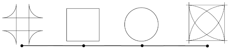
Figure 1. The convex segment between the disc and the square is extended until we arrive at two objects of zero (formal) area. The hyperbolic distance between the disc and the square is half of the logarithm of the cross-ratio of the four points.

In the first part of the present article, we bring this real hyperbolization process to its full generality, by endowing the space of convex bodies in $\mathbb{R}^{n}$ with an “area distance”, which appears to be hyperbolic in a sense clarified below. The idea behind the definition of the area distance is quite natural. Consider the convex combination $K_{t}=tK_{1}+(1-t)K_{2}$, of two convex bodies, $t\in[0,1]$. In general, by Alexandrov–Fenchel Inequality, there exists $t_{0},t_{1}\in\mathbb{R}$, $t_{0}\leq 0<1\leq t_{1}$ such that the formal area of $K_{t}$ is zero. We then have two points ($0$ and $1$) on the segment $[t_{0},t_{1}]$, and, heuristically, $t_{0}$ and $t_{1}$ belong to the isotropic cone of a quadratic form (the area). Mimicking the definition of the distance of the Klein model of the hyperbolic space, we define the area distance as half of the log of the cross-ratio of $t_{0},0,1,t_{1}$, see Figure 1. See also Figure 5. The precise definition of the area distance will be given in Section 2.1.

Recall that two subsets $A$ and $B$ of $\mathbb{R}^{n}$ are homothetic if they differ by a translation and a positive scaling. If $K$ is a convex body, we denote by $[K]$ its homothety class, and by $\mathscr{H}\emph{om}^{n*}$ the space of homothety classes of all the convex bodies in $\mathbb{R}^{n}$, which are different from points and segments. The area distance introduced above is clearly invariant under homotheties. Let us denote by $d_{\mathscr{H}^{n}}$ the induced area distance on $\mathscr{H}\emph{om}^{n*}$. Note that it is not obvious that this is actually a distance.

Theorem 1.

$(\mathscr{H}\emph{om}^{n*},d_{\mathscr{H}^{n}})$ is a metric space which

1. is uniquely geodesic, and the unique shortest path between $[K_{1}]$ and $[K_{2}]$ is the class of the convex combination of $K_{1}$ and $K_{2}$,

2. is of infinite Hausdorff dimension and infinite diameter,

3. is proper,

4. has curvature bounded from below and above by $-1$ in the sense of Alexandrov,

5. has boundary homeomorphic to the real projective space of dimension $(n-1)$,

6. any point is the endpoint of a shortest path that is not extendable beyond this point,

7. is homeomorphic to the space of convex bodies of intrinsic area equal to one and Steiner point at the origin, endowed with the Hausdorff distance.

As some definitions may depend on the authors, let us recall that a metric space is geodesic if any two points are joined by a shortest path, it is uniquely geodesic if the shortest path is unique; and it is proper if every bounded closed subset is compact. A proper metric space is locally compact and complete. A shortest path is extendable if it is strictly contained in another shortest path. The boundary of a metric space is the set of equivalence classes of geodesic rays at bounded distance, endowed with a natural topology, see [5] for details. In the present article, the definition of bounded curvature in the sense of Alexandrov is global.

The property (6) is proved in Section 2.5. The topological properties in Theorem 1 are consequences of a theorem of R.A. Vitale and the Blaschke Selection Theorem, see Section 2.6. The other assertions in Theorem 1 are either straightforward, or they come from the following extrinsic description of $(\mathscr{H}\emph{om}^{n*},d_{\mathscr{H}^{n}})$.

Theorem 2.

$(\mathscr{H}\emph{om}^{n*},d_{\mathscr{H}^{n}})$ is isometric to an infinite dimensional unbounded closed convex subset with empty interior of the infinite dimensional hyperbolic space.

Here, “the” infinite dimensional hyperbolic space is defined from a separable Hilbert space. The isometry in Theorem 2 is obtained by considering the support function of convex bodies. Under this identification, the area of convex bodies will give a bilinear form, that appears to have a Lorentzian signature. This is actually very natural, as for example, Alexandrov–Fenchel Inequality for mixed-area is then given by a reversed Cauchy–Schwarz Inequality.

We say that the distance $d_{\mathscr{H}^{n}}$ is hyperbolic, because it is isometric to a totally geodesic subspace of an hyperbolic space, or because of the curvature property (4) in Theorem 1 (the latter being an immediate consequence of the former). Note that for metric spaces, it is meaningless to speak about “curvature equal to $-1$”.

It was pointed out by Nicolas Monod to the second author that the present construction for $n=2$ gives an explicit example of an exotic action of $PSL(2,\mathbb{R})$ on the infinite dimensional hyperbolic space [18].

In the second part of the present article, we investigate $\mathscr{S}\emph{hape}^{n*}$, the quotient of $\mathscr{H}\emph{om}^{n*}$ by linear isometries of the Euclidean space $\mathbb{R}^{n}$: $\mathscr{S}\emph{hape}^{n*}$ is the space of convex bodies in $\mathbb{R}^{n}$ (not reduced to points or segments) up to Euclidean similarities (such an equivalence class is the “shape” of the convex body). It is endowed with the quotient distance $d_{\mathscr{S}^{n}}$. We obtain the following.

Theorem 3.

$(\mathscr{S}\emph{hape}^{n*},d_{\mathscr{S}^{n}})$ is a proper geodesic metric space with curvature $\geq-1$ and with boundary reduced to a single point. It is not uniquely geodesic. It contains many totally geodesic hyperbolic surfaces.

There is another complex hyperbolic orbifold considered by Thurston, which is defined similarly to the space $P$ introduced at the beginning of the present article, but where the singular points are not labeled. It is a subspace of $\mathcal{M}_{\geq 0}^{1}(\mathbb{S}^{2})$, the space of metrics of non-negative curvature on the sphere, up to isometries, and with unit area. A natural generalization of Thurston construction would be to use the area of the metrics to endow $\mathcal{M}_{\geq 0}^{1}(\mathbb{S}^{2})$ with a distance, and look at its properties. For example, one may look at curvature properties, or possible complex structure. From [3] and (7) in Theorem 1, it follows that $\mathscr{S}\emph{hape}^{3*}$ and $\mathcal{M}_{\geq 0}^{1}(\mathbb{S}^{2})$ are homeomorphic, if the latter space is endowed with the topology of uniform convergence of distances. So Theorem 3, for $n=3$, may be seen as a “real hyperbolization” of $\mathcal{M}_{\geq 0}^{1}(\mathbb{S}^{2})$ with its natural topology. Here the word “hyperbolization” is used in a wide sense, as as $(\mathscr{S}\emph{hape}^{n*},d_{\mathscr{S}^{n}})$ is not uniquely geodesic, it is not of non-positive curvature, hence not with curvature $\leq-1$. However that’s an open question to know if it is locally of non-positive curvature.

We conclude the present article by a question about the space of shapes of all convex bodies (regardless of the dimension of the ambient space).

As we pointed out, the idea to consider convex bodies in an ambient hyperbolic space came from the observation that the Alexandrov–Fenchel Inequality for the mixed-area of convex bodies looks like the reversed Cauchy–Schwarz Inequality in a Lorentzian vector space (see Remark 2.19). In dimension $2$, Alexandrov–Fenchel Inequality coincides with the Minkowski inequality. Also, mixed-volumes were introduced by Minkowski. He also introduced Lorentzian vector spaces, which are now called Minkowski spaces. We are not aware if Minkowski knew a relation between the inequality and the spaces that both bear his name. But as far as we know, it seems that in the meantime this relation between the fundamental inequality of the theory of convex bodies and basic Lorentzian geometry was forgotten.

Acknowledgements.

The authors want to thank Nicola Gigli, Julien Maubon, Nicolas Monod, Graham Smith, Pierre-Damien Thizy and Giona Veronelli for useful conversations. They also want to thank Igor Belegradek who helped to clarify some points in a preceding version of the text. This work was completed during a visit of the second author at SISSA. He wants to thank the institution for its hospitality.

2. The area distance

2.1. Intrinsic area of convex bodies

A convex body is a non-empty compact convex subset of $\mathbb{R}^{n}$. In the present article, we set $n>1$. For a plane convex body $K$ (i.e. a convex body in $\mathbb{R}^{2}$), speaking about the “area” of $K$ usually means to look at its volume (two dimensional Lebesgue measure). Note that the area of plane convex bodies is positively homogeneous of degree $2$: for $\lambda>0$, $\operatorname{vol}_{2}(\lambda K)=\lambda^{2}\operatorname{vol}_{2}(K)$. For a convex body in $\mathbb{R}^{3}$, the “area” usually refers to its surface area, i.e. the $2$-dimensional total Hausdorff measure of its boundary $\partial K$. Here also, the surface area is positively homogeneous of degree two.

For $n>3$, there are two ways to generalize the notion of “area” to convex bodies in $\mathbb{R}^{n}$. Both are coming from the Steiner Formula. Let $B^{n}$ be the closed unit ball centered at the origin in $\mathbb{R}^{n}$, and let $\kappa_{n}$ be its volume. Let us set $\kappa_{0}=1$ and $\kappa_{1}=2$. If $K$ is a convex body in $\mathbb{R}^{n}$, then there exist non-negative real numbers $V_{i}(K)$, $i=0,\ldots,n$ such that, for any $\epsilon>0$,

(2.1) $$\mathrm{vol}_{n}(K+\epsilon B^{n})=\sum_{i=0}^{n}\epsilon^{n-i}\kappa_{n-i}V_{i}(K)~{}.$$

Here $\mathrm{vol}_{n}$ is the Lebesgue measure of $\mathbb{R}^{n}$, and the sum is the Minkowski addition: $A+B=\{a+b|a\in A,b\in B\}$. It appears that $V_{0}(K)=1$ and $V_{n}(K)=\mathrm{vol}_{n}(K)$.

The first way to generalize the notion of surface area of convex bodies in $\mathbb{R}^{3}$ is to consider $V_{n-1}(K)$ as the “area”, given by the first order variation of $\operatorname{vol}_{n}(K+\epsilon B^{n})$, seen as a function of $\epsilon$. Note that this “area” is homogeneous of degree $(n-1)$, and that for $n=2$, this is related to the perimeter of the convex body and not to its area.

In the present article, we consider another way to generalize the notion of surface area of convex bodies in $\mathbb{R}^{3}$, and we call $V_{2}(K)$ given by (2.1) the intrinsic area of $K$. Let us mention some relevant properties. The property A6) explains the terminology “intrinsic”.

1. For any $\lambda>0$, $V_{2}(\lambda K)=\lambda^{2}V_{2}(K)$;

2. $V_{2}(K)\geq 0$;

3. $K_{1}\subset K_{2}\Rightarrow V_{2}(K_{1})\leq V_{2}(K_{2})$;

4. $V_{2}(K)=0$ if and only if $K$ is a point or a segment;

5. for any $A\in O(n)$ and $p\in\mathbb{R}^{n}$, $V_{2}(A(K)+\{p\})=V_{2}(K)$;

6. Let $\iota:\mathbb{R}^{n}\to\mathbb{R}^{n+1}$ be a linear isometric embedding. Then $V_{2}(\iota(K))=V_{2}(K)$.

The (intrinsic) area can be “polarized”, in the sense that there exists a function called the (intrinsic) mixed-area $V_{2}(\cdot,\cdot)$, that can be defined as

(2.2) $$V_{2}(K_{1},K_{2})=\frac{1}{2}\left(V_{2}(K_{1}+K_{2})-V_{2}(K_{1})-V_{2}(K_{2})\right)~{},$$

and satisfies the following properties:

1. $V_{2}(K_{1},K_{1})=V_{2}(K_{1})$;

2. $V_{2}(K_{1},K_{2})=V_{2}(K_{2},K_{1})$;

3. $V_{2}(K_{1}+K_{2},K_{3})=V_{2}(K_{1},K_{3})+V_{2}(K_{2},K_{3})$;

4. for $\lambda>0$, $V_{2}(\lambda K_{1},K_{2})=\lambda V_{2}(K_{1},K_{2})$;

5. $K_{1}\subset K_{2}\Rightarrow V_{2}(K_{1},K_{3})\leq V_{2}(K_{2},K_{3})$;

6. $K$ is a point if and only if for any convex body $Q$, $V_{2}(K,Q)=0$;

7. $V_{2}(K_{1},K_{2})\geq 0$; and $V_{2}(K_{1},K_{2})=0$ if and only if $K_{1}$ or $K_{2}$ is a point, or both are segments with the same direction;

8. we have

   (2.3) $$\delta(K_{1},K_{2})=V_{2}(K_{1},K_{2})^{2}-V_{2}(K_{1})V_{2}(K_{2})\geq 0$$

   and if $K_{1}$ and $K_{2}$ are not points, then equality occurs if and only if $K_{1}$ and $K_{2}$ are homothetic.

All those properties are classical, as $V_{2}$ is a particular case of mixed-volume: $V_{2}(K_{1},K_{2})=V(K_{1},K_{2},B^{n},\ldots,B^{n})$ [20]. Property M8) is Alexandrov–Fenchel Inequality. In the present article, we will generalize the properties listed above, using some simple analysis of functions on the sphere. Before that, let us introduce the area distance on the space of homothety classes of convex bodies. We will give two equivalent definitions, both using Alexandrov–Fenchel Inequality M8).

In the sequel, we denote by $\mathcal{K}^{n}$ the set of convex bodies in $\mathbb{R}^{n}$, and by $\mathcal{K}^{n*}$ the subset of convex bodies of positive intrinsic area. In other terms, by A2) and A4), $\mathcal{K}^{n*}$ is $\mathcal{K}^{n}$ minus points and segments. By property M8) of the mixed-area, for any $K_{1},K_{2}\in\mathcal{K}^{n*}$, the quantity

$$\tilde{d}_{1}(K_{1},K_{2})=\operatorname{argch}\left(\frac{V_{2}(K_{1},K_{2})}{\sqrt{V_{2}(K_{1})V_{2}(K_{2})}}\right)~{}$$

is well-defined. This is also clear that $\tilde{d}_{1}(K_{1},K_{2})$ is invariant under positive scaling of $K_{1}$ and $K_{2}$. Moreover, by A5) and (2.2), for all $p\in\mathbb{R}^{n}$,

$$V_{2}(K_{1}+\{p\},K_{2})=V_{2}(K_{1},K_{2}+\{p\})=V_{2}(K_{1},K_{2})~{},$$

hence $\tilde{d}_{1}$ is invariant under translations of $K_{1}$ or $K_{2}$. By the case of equality in property M8), $\tilde{d}_{1}(K_{1},K_{2})=0$ if and only if $K_{1}$ differ from $K_{2}$ by a homothety.

Let us define the space $\mathscr{H}\emph{om}^{n}$ (resp. $\mathscr{H}\emph{om}^{n*}$) as the quotient of $\mathcal{K}^{n}$ (resp. $\mathcal{K}^{n*}$) by homotheties. For a convex body $K$, we denote by $[K]$ the set of homothetic copies of $K$. For any $[K_{1}],[K_{2}]\in\mathscr{H}\emph{om}^{n*}$ we set

$$d_{1}([K_{1}],[K_{2}])=\tilde{d}_{1}(K_{1},K_{2})~{}.$$

Let us do it in a different way. Let $K_{1},K_{2}\in\mathcal{K}^{n*}$. Assume that $V_{2}(K_{1})=V_{2}(K_{2})=a>0$ and that $[K_{1}]\neq[K_{2}]$. Consider the following equation:

(2.4) $$V_{2}((1-t)K_{1}+tK_{2})=0~{}.$$

By properties of the mixed-area, the left-hand side is a polynomial in $t$, and the coefficient of $t^{2}$ is $2a-2V_{2}(K_{1},K_{2})$. Since $[K_{1}]\neq[K_{2}]$, by Alexandrov-Fenchel Inequality M8), we have $V_{2}(K_{1},K_{2})>a$: the coefficient of $t^{2}$ is negative, in particular this is a second order polynomial. An easy calculation shows that its discriminant is equal to $4\delta(K_{1},K_{2})>0$ (see (2.3)). Let $t_{1}<0<1<t_{2}$ be the two real solutions of the equation (2.4), and let us define

$$\tilde{d}_{2}(K_{1},K_{2})=\frac{1}{2}\ln[0,1,t_{1},t_{2}]~{},$$

where $[0,1,t_{1},t_{2}]=\frac{t_{1}}{t_{2}}\frac{1-t_{2}}{1-t_{1}}$ is the cross-ratio.

By (2.4), it is clear that $\tilde{d}_{2}$ is invariant by translation of $K_{1}$ or $K_{2}$. Let $[K_{1}],[K_{2}]\in\mathscr{H}\emph{om}^{n*}$, and let $K_{1},K_{2}$ be two representatives having the same intrinsic area. We can then define

$$d_{2}([K_{1}],[K_{2}])=\tilde{d}_{2}(K_{1},K_{2})~{},$$

if $[K_{1}]\not=[K_{2}]$, and zero otherwise.

Classical trigonometry computations from hyperbolic geometry show $d_{1}=d_{2}$. We define the area distance on $\mathscr{H}\emph{om}^{n*}$ as

$$d_{\mathscr{H}^{n}}:=d_{1}=d_{2}~{}.$$

(Note that we didn’t proved yet that it is a distance.)

Even if the space of convex bodies is not a vector space, from its properties the mixed-area reminds a symmetric bilinear form, whose kernel is the space of points, and whose isotropic cone is the space of points and segments. Moreover, Alexandrov–Fenchel Inequality (2.3) reminds a reversed Cauchy–Schwarz Inequality. To define $d_{1}$ and $d_{2}$ above, we mimicked the definitions of the hyperboloid model and the Klein model of the hyperbolic space. It is actually the way we will prove Theorem 1.

2.2. Spaces of support functions

\psfrag{C}{$\mathcal{C}_{n}$}\psfrag{K}{$\mathbb{K}\mathbf{lein}^{\infty}_{n}$}\psfrag{H}{$\mathcal{H}_{n}^{\infty}$}\psfrag{H+}{$\mathbf{mean}>0$}\psfrag{H01}{$H^{1}(\mathbb{S}^{n-1})_{01}$}\psfrag{L}{$\operatorname{L}$}\psfrag{1}{}\psfrag{c}{}\psfrag{P}{}\psfrag{V1}{$\overline{V_{1}}^{n}=1$}\psfrag{V}{$\overline{V_{1}}^{n}=0$}\includegraphics[width=216.81pt]{Hyperbola}

Figure 2. Notations for subspaces of $H^{1}(\mathbb{S}^{n-1})_{1}$.

The support function $\operatorname{Supp}(K)$ of a convex body $K$ in $\mathbb{R}^{n}$ gives, at the point $x\in\mathbb{S}^{n-1}$, the distance from the origin of $\mathbb{R}^{n}$ to the support hyperplane of $K$ with outward normal $x$. More precisely, $\operatorname{Supp}(K):\mathbb{S}^{n-1}\to\mathbb{R}$ is defined as

$$\operatorname{Supp}(K)(x)=\max_{p\in K}\langle x,p\rangle~{},$$

where $\langle\cdot,\cdot\rangle$ is the usual scalar product of $\mathbb{R}^{n}$.

Let us denote by $\|\cdot\|_{L^{2}}$ the $L^{2}$ norm on the round sphere $\mathbb{S}^{n-1}$. Let $H^{1}(\mathbb{S}^{n-1})$ be the Sobolev space of $\mathbb{S}^{n-1}$, i.e. the space of functions $\mathbb{S}^{n-1}\to\mathbb{R}$ which are in $L^{2}(\mathbb{S}^{n-1})$ as well as their first order derivatives in the weak sense. The space $H^{1}(\mathbb{S}^{n-1})$ is implicitly endowed with the norm

$$\|h\|_{H^{1}}=\left(\|h\|_{L^{2}}^{2}+\|\nabla h\|_{L^{2}}^{2}\right)^{1/2}=\left(\int_{\mathbb{S}^{n-1}}h^{2}+\|\nabla h\|^{2}\right)^{1/2}$$

where the gradient $\nabla$ is the one of the round sphere.

If $K$ is contained in the ball centered at the origin and with radius $R$, then $\operatorname{Supp}(K)$ is $R$-Lipschitz. Hence we get a map

$$\operatorname{Supp}:\mathcal{K}^{n}\to H^{1}(\mathbb{S}^{n-1})~{}.$$

Let us recall some basic properties [20, 10, 11]:

• a function $h:\mathbb{S}^{n-1}\to\mathbb{R}$ is the support function of a convex body in $\mathbb{R}^{n}$ if and only if its one homogeneous extension $\tilde{h}:\mathbb{R}^{n}\setminus\{0\}\to\mathbb{R}$, $\tilde{h}(x)=\|x\|h(x/\|x\|)$, $\tilde{h}(0)=0$, is a convex function;

• $\operatorname{Supp}(K_{1}+K_{2})=\operatorname{Supp}(K_{1})+\operatorname{Supp}(K_{2})$, $\operatorname{Supp}(\lambda K)=\lambda\operatorname{Supp}(K)$, $\lambda>0$; in particular, $\operatorname{Supp}(\mathcal{K}^{n})$ is a convex cone in $H^{1}(\mathbb{S}^{n-1})$.

• $\operatorname{Supp}$ is a bijection onto its image;

• if $K_{1}\subset K_{2}$, then $\operatorname{Supp}(K_{1})\leq\operatorname{Supp}(K_{2})$;

• if $(\operatorname{Supp}(K_{i}))_{i}$ converges pointwise to $\operatorname{Supp}(K)$, then the convergence is uniform;

• if $(\operatorname{Supp}(K_{i}))_{i}$ converges to $\operatorname{Supp}(K)$, then almost everywhere $(\nabla\operatorname{Supp}(K_{i}))_{i}\to\nabla\operatorname{Supp}(K)$.

Remark 2.1.

Let us warn the reader that if $\operatorname{Supp}(\lambda K)=\lambda\operatorname{Supp}(K)$, $\lambda>0$, we don’t have $\operatorname{Supp}(-K)=-\operatorname{Supp}(K)$ in general, where $-K=\{-x|x\in K\}$. Indeed, both $\operatorname{Supp}(-K)$ and $\operatorname{Supp}(K)$ are positive if the origin of $\mathbb{R}^{n}$ is in the interior of $K$. Actually, $\operatorname{Supp}(-K)(v)=\operatorname{Supp}(K)(-v)$, and $-\operatorname{Supp}(K)$ is like the support function of $K$, but with the support planes defined by their inward unit normals.

Let us set $\lambda_{1}=n-1$ and $c_{n}$ be a given positive constant. For $h\in H^{1}(\mathbb{S}^{n-1})$, let us consider the quadratic form

(2.5) $$\overline{V_{2}}^{n}(h)=c_{n}\left(\|h\|_{L^{2}}^{2}-\lambda_{1}^{-1}\|\nabla h\|_{L^{2}}^{2}\right)~{},$$

that comes from the following bilinear form: for $h,k\in H^{1}(\mathbb{S}^{n-1})$,

$$\overline{V_{2}}^{n}(h,k)=c_{n}\left(\mathbf{(}h,k\mathbf{)}_{L^{2}}-\lambda_{1}^{-1}(\nabla h,\nabla k)_{L^{2}}\right)~{}.$$

To avoid confusion, let us emphasis that $\overline{V_{2}}^{n}(h,h)=\overline{V_{2}}^{n}(h).$ It is known (see e.g. [11, Theorem 4.2a], [20, p. 298] or [10, Proposition 2.4.2]) that for any $n$ there is a unique $c_{n}$ such that, for any $K_{1},K_{2}\in\mathcal{K}^{n}$

$$V_{2}(K_{1},K_{2})=c_{n}\overline{V_{2}}^{n}(\operatorname{Supp}(K_{1}),\operatorname{Supp}(K_{2}))~{}.$$

Let us first restrict $\overline{V_{2}}^{n}$ to a subspace where it is not degenerate. Hopefully, the kernel of $\overline{V_{2}}^{n}$ is exactly the image of points by $\operatorname{Supp}$. Indeed, the support function of the point $p\in\mathbb{R}^{n}$ is the restriction to the sphere of the linear map $x\mapsto\langle p,x\rangle$. But the space of such maps is the eigenspace of the first non-zero eigenvalue of the Laplacian on the round sphere, and this eigenvalue is the $\lambda_{1}$ in (2.5), so we deduce easily the following fact.

Fact 2.2.

The kernel of $\overline{V_{2}}^{n}(\cdot,\cdot)$ on $H^{1}(\mathbb{S}^{n-1})$ is the eigenspace of $\lambda_{1}$.

Proof.

Let $h\in H^{1}(\mathbb{S}^{n-1})$. The function $h$ belongs to the kernel of $\overline{V_{2}}^{n}(\cdot,\cdot)$ if and only if for any $k\in H^{1}(\mathbb{S}^{n-1})$ we have

$$\int_{\mathbb{S}^{n-1}}hk=\lambda_{1}^{-1}\int_{\mathbb{S}^{n-1}}\langle\nabla h,\nabla k\rangle~{}.$$

By density of smooth functions on $\mathbb{S}^{n-1}$ for the $H^{1}$-norm and by Green Formula, this is equivalent to the following property: for any smooth function $k$ on $\mathbb{S}^{n-1}$ we have

$$\int_{\mathbb{S}^{n-1}}hk=\lambda_{1}^{-1}\int_{\mathbb{S}^{n-1}}h\Delta k~{},$$

and this means $h=\lambda_{1}^{-1}\Delta h$ in the weak (hence smooth) sense. ∎

We will denote by $H^{1}(\mathbb{S}^{n-1})_{1}$ the subspace of $H^{1}(\mathbb{S}^{n-1})$ of functions $L^{2}$-orthogonal to the eigenspace of $\lambda_{1}$, i.e.

$$H^{1}(\mathbb{S}^{n-1})_{1} = \{h\in H^{1}(\mathbb{S}^{n-1})|\left(h,x^{i}\right)_{L^{2}}=0~{},i=1,\ldots,n\}$$

$$= \{h\in H^{1}(\mathbb{S}^{n-1})|\int_{\mathbb{S}^{n-1}}h(x)x\,\mbox{d}\mathbb{S}^{n-1}(x)=0\}~{}.$$

In turn, $\overline{V_{2}}^{n}$ is non-degenerate on $H^{1}(\mathbb{S}^{n-1})_{1}$. This space has a clear geometric meaning for convex bodies. Recall that the Steiner point of a convex body $K$ is the following point of $\mathbb{R}^{n}$:

$$\mathbf{stein}(K)=\frac{1}{\kappa_{n}}\int_{\mathbb{S}^{n-1}}\operatorname{Supp}(K)(x)x\mbox{d}\mathbb{S}^{n-1}~{},$$

so that

$$\mathbf{stein}(K)=0\Longleftrightarrow\operatorname{Supp}(K)\in H^{1}(\mathbb{S}^{n-1})_{1}~{}.$$

We have that for any $p\in\mathbb{R}^{n}$, $\mathbf{stein}(K+\{p\})=\mathbf{stein}(K)+\{p\}$, hence a convex body with Steiner point at the origin is a representative of the class of this convex body up to translations.

Now we prove that $\overline{V_{2}}^{n}$ has a Lorentzian signature on $H^{1}(\mathbb{S}^{n-1})_{1}$: it is positive in one direction, and negative-definite on the orthogonal (for a given scalar product, here the Sobolev one). Let $\operatorname{L}$ be the line of constant functions in $H^{1}(\mathbb{S}^{n-1})_{1}$. We denote by $H^{1}(\mathbb{S}^{n-1})_{01}$ the subspace of $H^{1}(\mathbb{S}^{n-1})_{1}$ of elements $H^{1}$ (or, equivalently, $L^{2}$) orthogonal to $\operatorname{L}$.

Lemma 2.3.

For $h\in H^{1}(\mathbb{S}^{n-1})_{01}$,

(2.6) $$c_{n}\left(\frac{\lambda_{2}-\lambda_{1}}{\lambda_{1}}\right)\|h\|_{L^{2}}^{2}\leq-\overline{V_{2}}^{n}(h)$$

and

(2.7) $$c_{n}\left(\frac{\lambda_{2}-\lambda_{1}}{\lambda_{1}\lambda_{2}}\right)\|h\|^{2}_{H^{1}}\leq-\overline{V_{2}}^{n}(h)\leq c_{n}\frac{1}{\lambda_{1}}\|h\|^{2}_{H^{1}}~{}.$$

Proof.

The space $\operatorname{L}$ is exactly the eigenspace of the zero eigenvalue of the spherical Laplacian. If we denote by $\lambda_{2}(>\lambda_{1})$ the second positive eigenvalue, then by Rayleigh Theorem, for $h\in H^{1}(\mathbb{S}^{n-1})_{01}\setminus\{0\}$ we have

(2.8) $$\lambda_{2}\leq\frac{\|\nabla h\|_{L^{2}}^{2}}{\|h\|_{L^{2}}^{2}}~{}.$$

Now (2.6) is immediate from (2.8), and the right-hand side inequality in (2.7) follows from

$$-\overline{V_{2}}^{n}(h)\leq c_{n}\lambda_{1}^{-1}\|\nabla h\|^{2}_{L^{2}}\leq c_{n}\lambda_{1}^{-1}\|h\|^{2}_{H^{1}}~{}.$$

The left-hand side inequality in (2.7) follows by adding the two following inequalities: as $\lambda_{2}>\lambda_{1}=n-1\geq 1$, (2.6) gives

$$c_{n}\frac{1}{\lambda_{2}}\left(\frac{\lambda_{2}-\lambda_{1}}{\lambda_{1}}\right)\|h\|^{2}_{L^{2}}\leq-\overline{V_{2}}^{n}(h)~{},$$

and on the other hand, using again (2.8), the equality (2.5) gives

$$c_{n}\left(\frac{1}{\lambda_{1}}-\frac{1}{\lambda_{2}}\right)\|\nabla h\|_{L^{2}}^{2}\leq-\overline{V_{2}}^{n}(h)~{}.$$

∎

Clearly $\overline{V_{2}}^{n}$ is positive definite on $\operatorname{L}$, and we have:

Proposition 2.4.

$(H^{1}(\mathbb{S}^{n-1})_{01},-\overline{V_{2}}^{n}(\cdot,\cdot))$ is a separable Hilbert space.

Proof.

By (2.6) or (2.7), $-\overline{V_{2}}^{n}$ is a scalar product on $H^{1}(\mathbb{S}^{n-1})_{01}$. As $H^{1}(\mathbb{S}^{n-1})_{01}$ is orthogonal to a vector subspace, it is a closed subspace, hence complete and separable for the $H^{1}$ norm. The result follows from (2.7). ∎

Note that as $\overline{V_{2}}^{n}$ is Lorentzian on $H^{1}(\mathbb{S}^{n-1})_{1}$, we obtain the reversed Cauchy–Schwarz Inequality, that generalizes Alexandrov–Fenchel Inequality M8):

(2.9) $$\overline{V_{2}}^{n}(h,k)^{2}\geq\overline{V_{2}}^{n}(h)\overline{V_{2}}^{n}(k)~{},$$

for $h,k\in\mathcal{C}_{n}$ with (see Figure 2)

$$\mathcal{C}_{n}=\{h\in H^{1}(\mathbb{S}^{n-1})_{1}|\overline{V_{2}}^{n}(h)>0,\overline{V_{1}}^{n}(h)>0\}~{},$$

and where

$$\overline{V_{1}}^{n}(h)=\frac{1}{\kappa_{n-1}}\int_{\mathbb{S}^{n-1}}h~{},$$

and equality occurs in (2.9) if and only if $h=\lambda k$, $\lambda>0$.

Let us mention that it is known that, for a convex body $K\subset\mathbb{R}^{n}$, if $V_{1}(K)$ is given by (2.1), then

$$V_{1}(K)=\overline{V_{1}}^{n}(\operatorname{Supp}(K))~{}.$$

2.3. Infinite dimensional hyperbolic space

Let us introduce

$$\mathcal{H}_{n}^{\infty}=\{h\in\mathcal{C}_{n}|\overline{V_{2}}^{n}(h)=1\}~{}.$$

As the Hilbert structure on $H^{1}(\mathbb{S}^{n-1})_{01}$ is given by $\overline{V_{2}}^{n}$, the map $\overline{V_{2}}^{n}$ is smooth, and it is easy to see that $\mathcal{H}_{n}^{\infty}$ is the graph of a smooth map over $H^{1}(\mathbb{S}^{n-1})_{01}$, hence an infinite dimensional smooth manifold. We implicitly endow $\mathcal{H}_{n}^{\infty}$ with the restriction of $-\overline{V_{2}}^{n}(\cdot,\cdot)$ on its tangent spaces. The intersection of $\mathcal{H}_{n}^{\infty}$ with any vector subspace of finite dimension $p$ of $H^{1}(\mathbb{S}^{n-1})_{1}$ containing a vector of $\mathcal{C}_{n}$, is clearly a hyperboloid model of the hyperbolic space of dimension $(p-1)$. In turn, $\mathcal{H}_{n}^{\infty}$ is a Riemannian manifold of constant sectional curvature $-1$. Moreover, it is not hard to see that the map $\mathbf{p}_{\mathcal{H}}:\mathcal{H}_{n}^{\infty}\rightarrow H^{1}(\mathbb{S}^{n-1})_{01}$, $\mathbf{p}_{\mathcal{H}}(h)=h-\frac{\overline{V_{1}}^{n}(h)}{\overline{V_{1}}^{n}(1)}$ is bijection and locally bi-Lipschitz, so by Proposition 2.4, $\mathcal{H}_{n}^{\infty}$ is complete.

Let us denote by $d_{\mathcal{H}}$ the distance induced by the Riemannian structure, and we have, in the same way than in the finite dimensional case,

$$d_{\mathcal{H}}(h,k)=\operatorname{argch}\overline{V_{2}}^{n}\left(h,k\right)~{}.$$

We will also need the pull-back of the distance on the hyperboloid onto

$$\mathbb{K}\mathbf{lein}^{\infty}_{n}=\{h\in\mathcal{C}_{n}~{}|~{}\overline{V_{1}}^{n}(h)=1\}~{}$$

via a central projection, i.e. the hyperbolic distance on $\mathbb{K}\mathbf{lein}^{\infty}_{n}$ is defined by

(2.10) $$d_{\mathbb{K}}(h,k):=d_{\mathcal{H}}(\overline{V_{2}}^{n}(h)^{-1/2}h,\overline{V_{2}}^{n}(k)^{-1/2}k)~{}.$$

Of course it is possible to write $d_{\mathbb{K}}$ in an intrinsic way, as we did in Section 2.1 for the area distance, using (2.9) instead of M8). For future references let us note the following non-surprising facts, whose proofs are left to the reader.

Fact 2.5.

On $\mathcal{H}_{n}^{\infty}$, $d_{\mathcal{H}}$ and $d_{H^{1}}$ induce the same topology, where $d_{H^{1}}$ is the distance induced by $\|\cdot\|_{H^{1}}$.

Fact 2.6.

Let $h_{i},k\in\mathbb{K}\mathbf{lein}^{\infty}_{n}$. Then

$$\overline{V_{2}}^{n}(h_{i})\to 0\iff d_{\mathbb{K}}(h_{i},k)\to+\infty~{}.$$

Fact 2.7.

Let $(h_{i})_{i}$ converge to $h$ in $(\mathbb{K}\mathbf{lein}^{\infty}_{n},d_{\mathbb{K}})$. Then $\overline{V_{2}}^{n}(h-h_{i})\to 0$.

Fact 2.8.

On $\mathbb{K}\mathbf{lein}^{\infty}_{n}$, $d_{\mathbb{K}}$ and $d_{H^{1}}$ induce the same topology.

2.4. Spaces of convex bodies

Recall that $\mathcal{K}^{n}$ (resp. $\mathcal{K}^{n*}$) is the set of convex bodies in $\mathbb{R}^{n}$ (resp. convex bodies with positive intrinsic area). We denote by $\mathcal{K}^{n}_{S}$ the space of convex bodies with Steiner point at the origin, and $\mathcal{K}^{n*}_{S}=\mathcal{K}^{n}_{S}\cap\mathcal{K}^{n*}$.

In the sequel, a star as upper-script mean that we consider only convex bodies with positive intrinsic area (that is, we exclude points and segments). In the following table, it is obvious that all the sets without a star are in bijection, as well as all the sets with a star.

convex bodies	up to positive	with $V_{2}=1$	with $V_{1}=1$
in $\mathbb{R}^{n}$…	scaling
up to translations	$\mathscr{H}\emph{om}^{n}$ and $\mathscr{H}\emph{om}^{n*}$
with Steiner point		$\mathcal{K}^{n}_{SV_{2}}$ and $\mathcal{K}^{n*}_{SV_{2}}$	$\mathcal{K}^{n}_{SV_{1}}$ and $\mathcal{K}^{n*}_{SV_{1}}$
at the origin

We have

$\operatorname{Supp}(\mathcal{K}_{S}^{n*})\subset\mathcal{C}_{n}$,

$\operatorname{Supp}(\mathcal{K}^{n*}_{SV_{2}})\subset\mathcal{H}^{\infty}_{n}$,

$\operatorname{Supp}(\mathcal{K}^{n*}_{SV_{1}})\subset\mathbb{K}\mathbf{lein}^{\infty}_{n}$ .

Clearly, $\mathcal{K}^{n*}_{SV_{2}}$ (resp. $\mathcal{K}^{n*}_{SV_{1}}$) is in bijection with $\mathscr{H}\emph{om}^{n*}$, and we denote by $d_{SV_{2}}$ (resp. $d_{SV_{1}}$) the pull-back of $d_{\mathscr{H}^{n}}$ on $\mathcal{K}^{n*}_{SV_{2}}$ (resp. $\mathcal{K}^{n*}_{SV_{1}}$). By construction, the map $\operatorname{Supp}$ defines isometries

$$(\mathcal{K}^{n*}_{SV_{2}},d_{SV_{2}}) \overset{\sim}{\longrightarrow} (\operatorname{Supp}(\mathcal{K}^{n*}_{SV_{2}}),d_{\mathcal{H}})~{},$$

$$(\mathcal{K}^{n*}_{SV_{1}},d_{SV_{1}}) \overset{\sim}{\longrightarrow} (\operatorname{Supp}(\mathcal{K}^{n*}_{SV_{1}}),d_{\mathbb{K}})~{},$$

and as all these sets are isometric to $(\mathscr{H}\emph{om}^{n*},d_{\mathscr{H}^{n}})$. We immediately obtain some parts of Theorems 1 and 2: $(\mathscr{H}\emph{om}^{n*},d_{\mathscr{H}^{n}})$ is a metric space, isometric to a convex subset of $\mathbb{H}^{\infty}_{n}$. In turn, it has curvature $\leq-1$ and $\geq-1$, as this is clearly true for its isometric image in the hyperbolic space, and it is a uniquely geodesic metric space, as the hyperbolic space is uniquely geodesic. The unique shortest path is the convex combination, as the property occurs in $\mathbb{K}\mathbf{lein}^{\infty}_{n}$.

Let us check two easy facts that give other parts of Theorems 1 and 2. The first one implies that $\operatorname{Supp}(\mathcal{K}^{n*}_{SH})$ is unbounded.

Fact 2.9.

$\operatorname{Supp}(\mathcal{K}^{n*}_{SH})$ contains an entire geodesic of $\mathbb{H}_{n}^{\infty}$.

Proof.

In the plane, consider the following segments: $K_{1}=[-1,1]\times\{0\}$ and $K_{2}=\{0\}\times[-1,1]$. For $0\leq t\leq 1$, the convex combination $(1-t)K_{1}+tK_{2}$ is the rectangle $[-(1-t),1-t]\times[-t,t]$, whose Steiner point is $0$. This gives an entire geodesic of $\mathbb{H}_{2}^{\infty}$ contained in $\operatorname{Supp}(\mathcal{K}^{2*}_{SH})$. ∎

The following fact implies that $(\mathscr{H}\emph{om}^{n*},d_{\mathscr{H}^{n}})$ has infinite Hausdorff dimension.

Fact 2.10.

For any $s\in\mathbb{N}$, there is an open ball of the finite dimensional hyperbolic space $\mathbb{H}^{s}$ that isometrically embeds into $(\mathscr{H}\emph{om}^{n*},d_{\mathscr{H}^{n}})$.

Proof.

The convex hyperbolic polyhedra constructed in [2] parametrize the similarity classes of convex polygons with fixed angles; by construction, they isometrically embed into $(\mathscr{H}\emph{om}^{n*},d_{\mathscr{H}^{n}})$. The dimension of the hyperbolic polyhedra is $(s-3)$ if the polygons have $s$ edges. ∎

Fact 2.11.

The boundary of $(\mathscr{H}\emph{om}^{n*},d_{\mathscr{H}^{n}})$ is homeomorphic to the real projective space of dimension $(n-1)$

Proof.

The boundary is the space of segments, up to homotheties: indeed, for example by looking at the isometric model $(\operatorname{Supp}(\mathcal{K}_{SV_{1}}^{n*}),d_{\mathbb{K}})$, we see that the convex bodies $K$ on the boundary are the one for which $V_{2}(K)=0$ (see Fact 2.6) and $V_{1}(K)=1$, and these are exactly unit length segments. Hence $\partial\mathscr{H}\emph{om}^{n*}$ is in bijection with $P^{n-1}(\mathbb{R})$, the real projective space of dimension $n-1$ (that is, the space of lines in $\mathbb{R}^{n}$).

We can endow $\partial\mathscr{H}\emph{om}^{n*}$ with the visibility metric from $[B^{n}]$: the distance between $a,b\in\partial\mathscr{H}\emph{om}^{n*}$, denoted by $<_{B}(a,b)$, is the angle (with value in $[0,\pi]$) between the two lines $c_{a}$ and $c_{b}$ from $[B^{n}]$ and with endpoints $a$ and $b$ respectively. But clearly, the element of $O(n)$ sending the line $a$ to the line $b$ is also a $d_{\mathscr{H}^{n}}$-isometry sending $c_{a}$ to $c_{b}$. In turn, $\partial\mathscr{H}\emph{om}^{n*}$ endowed with the visibility metric is isometric to $P^{n-1}(\mathbb{R})$ endowed with its round metric. From [5, Proposition II.9.2], $<_{B}:\partial\mathscr{H}\emph{om}^{n*}\times\partial\mathscr{H}\emph{om}^{n*}\to\mathbb{R}$ is continuous for the classical topology on $\partial\mathscr{H}\emph{om}^{n*}$. Hence for this topology, $\partial\mathscr{H}\emph{om}^{n*}$ is homeomorphic to $P^{n-1}(\mathbb{R})$.

∎

In the two following sections we will prove the two remaining parts of Theorems 1 and 2: the assertion about terminal points of segments, and the topological properties.

2.5. Terminal points of segments

Let $K_{1},K_{2}\in\mathcal{K}_{SV_{1}}^{n}$. The segment between $K_{1}$ and $K_{2}$ is $\{(1-t)K_{1}+tK_{2},t\in[0,1]\}$. We say that $K_{1}\in\mathcal{K}_{SV_{1}}^{n}$ is a terminal point of the segment if for any $t<0$, $(1-t)\operatorname{Supp}(K_{1})+t\operatorname{Supp}(K_{2})\notin\operatorname{Supp}(\mathcal{K}_{SV_{1}}^{n})$. An extreme point $K$ of $\mathcal{K}_{SV_{1}}^{n}$ is such that there does not exist $K_{1},K_{2}\in\mathcal{K}_{SV_{1}}^{n}$, $K_{1}\not=K_{2}$, and $t\in(0,1)$ such that $\operatorname{Supp}(K)=(1-t)\operatorname{Supp}(K_{1})+t\operatorname{Supp}(K_{2})$. In the plane, extreme points of $\mathcal{K}_{SV_{1}}^{2}$ are segments and triangles [20, Theorem 3.2.14]. For $n\geq 3$, extreme points of $\mathcal{K}_{SV_{1}}^{n}$ are dense for the Hausdorff distance [20, 3.2.18].

Clearly, an extreme point is a terminal point for all the segments ending at this point. But there are much more terminal points. For example, one can find convex bodies with a non smooth point on the boundary (i.e. a point of the convex body contained in more than one support plane) which are terminal points for the segment starting at the unit ball —this idea is illustrated in Figure 3.

\psfrag{K}{$K$}\psfrag{e}{$\epsilon$}\psfrag{K+}{$K+\epsilon B^{2}$}\psfrag{K-}{$K-\epsilon B^{2}$}\includegraphics[width=173.44534pt]{terminal2}

Figure 3. If a plane convex body $K$ has a non-smooth point, then for any $\epsilon>0$, $\operatorname{Supp}(K)+\epsilon\operatorname{Supp}(B^{2})$ is the support function of a convex body, while $\operatorname{Supp}(K)-\epsilon\operatorname{Supp}(B^{2})$ is not.

In this section, we will use a different argument to prove that any convex body is the terminal point of some segment (Proposition 2.12), see Figure 4 for an example.

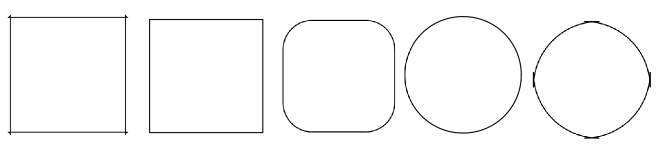
Figure 4. The disc and the square are both terminal points of the segment joining them.

If a function $h\in\mathbb{K}\mathbf{lein}^{\infty}_{n}$ belongs to $\operatorname{Supp}(\mathcal{K}_{SV_{1}}^{n*})$, then its one-homogeneous extension $\tilde{h}$ is convex, hence has non-negative Laplacian in the weak sense. This means that for every non-negative function $\varphi\in C^{\infty}_{c}(\mathbb{R}^{n})$, we have

$$\int_{\mathbb{R}^{n}}\tilde{h}(x)\Delta_{e}\varphi(x)\mbox{d}x\geq 0~{},$$

where $C^{\infty}_{c}(\mathbb{R}^{n})$ is the set of smooth functions with compact support in $\mathbb{R}^{n}$.

For $1\leq p<n$, we will denote by $B_{p,n}$ the $p$-dimensional ball with radius $r_{1}(p)$ in $\mathbb{R}^{n}$, which is the set of points $x\in\mathbb{R}^{n}$ with $x_{1}^{2}+\cdots+x_{p}^{2}\leq r_{1}(p)^{2}$ and $x_{p+1}=\cdots=x_{n}=0$. The number $r_{1}(p)$ is such that a ball with such radius has $V_{1}=1$. We have $V_{1}(B_{p,n})=1$, hence $B_{p,n}\in\mathcal{K}_{SV_{1}}^{n}$ (note that $B_{p,n}\in\mathcal{K}_{SV_{1}}^{n*}$ if and only if $p\geq 2$). Let $b_{p,n}=\operatorname{Supp}(B_{p,n})\in\operatorname{Supp}(\mathcal{K}_{SV_{1}}^{n})$ and let $\widetilde{b_{p,n}}(x)=r_{1}(p)\sqrt{x_{1}^{2}+\cdots+x_{p}^{2}}$ be the 1-homogeneous extension of $b_{p,n}$ (if $p=1$, then $\widetilde{b_{p}}(x)=r_{1}(1)|x_{1}|=\frac{|x_{1}|}{2}$).

Proposition 2.12.

Let $p\in\mathbb{N}$ such that $1\leq p<n$. Then any $K\in\mathcal{K}_{SV_{1}}^{n*}$ is the terminal point of a segment in $\mathcal{K}_{SV_{1}}^{n*}$, which starts at some embedded $p-$dimensional ball in $\mathbb{R}^{n}$.

Actually the proof will show that there are infinitely many such segments. If $p=1$, this ball is in fact a segment and lies on the boundary of $\mathbb{K}\mathbf{lein}^{\infty}_{n}$.

To prove Proposition 2.12, we need the following theorem due to Alexandrov (see [4]).

Theorem 2.13.

A convex function $f:\mathbb{R}^{n}\rightarrow\mathbb{R}$ is twice differentiable at almost every $\bar{x}\in\mathbb{R}^{n}$, which means that for almost every $\bar{x}\in\mathbb{R}^{n}$, there exists a quadratic polynomial $Q_{\bar{x}}$, and a function $R_{\bar{x}}$, such that

$$f(x)=Q_{\bar{x}}(x)+R_{\bar{x}}(x)\mbox{ and }\lim_{u\rightarrow 0}\frac{R_{\bar{x}}(\bar{x}+u)}{\|u\|^{2}}=0~{}.$$

Proof of Proposition 2.12.

Let $k=\operatorname{Supp}(K)\in\operatorname{Supp}(\mathcal{K}_{SV_{1}}^{n*})$, and let $\tilde{k}$ be its 1-homogeneous extension. Let $\bar{x}\in\mathbb{R}^{n}$ be a point at which $\tilde{k}$ is twice differentiable, and let $Q_{\bar{x}}$ and $R_{\bar{x}}$ be as in Theorem 2.13. Since $n>p$, the vector space $\{x_{1}=\cdots=x_{p}=0\}$ has positive dimension, hence, up to a rotation of $K$, we may assume that the first components of $\bar{x}$ are $\bar{x}_{1}=\cdots=\bar{x}_{p}=0$.

Let $\varphi\in C^{\infty}_{c}(\mathbb{R}^{n})$ be a non-negative function, with support in the unit ball in $\mathbb{R}^{n}$, positive in a neighborhood of $0$, and with $\int_{\mathbb{R}^{n}}\varphi=1$. For $\epsilon>0$, let $\varphi_{\epsilon}\in C^{\infty}_{c}(\mathbb{R}^{n})$ be the function $\varphi_{\epsilon}(x)=\frac{1}{\epsilon^{n}}\varphi(\frac{x-\bar{x}}{\epsilon})$: this function is non-negative, has support in $B(\epsilon,\bar{x})$ (the ball centered at $\bar{x}$ and with radius $\epsilon$), and $\int_{\mathbb{R}^{n}}\varphi_{\epsilon}=1$.

Let $t<0$. We want to show that $(1-t)k+tb_{p,n}\notin\operatorname{Supp}(\mathcal{K}_{SV_{1}}^{n*})$. We argue by contradiction: assume that $(1-t)k+tb_{p,n}\in\operatorname{Supp}(\mathcal{K}_{SV_{1}}^{n*})$. Then $(1-t)\tilde{k}+t\widetilde{b_{p,n}}$ is a convex function on $\mathbb{R}^{n}$, hence its Laplacian is non-negative in the weak sense, so in particular we have

(2.11) $$\int_{\mathbb{R}^{n}}((1-t)\tilde{k}+t\widetilde{b_{p,n}})\Delta_{e}\varphi_{\epsilon}\geq 0~{}.$$

We will first show that we always have

(2.12) $$\int_{\mathbb{R}^{n}}\tilde{k}\Delta_{e}\varphi_{\epsilon}\underset{\epsilon\rightarrow 0}{\longrightarrow}+\infty~{}.$$

Since $t$ is negative, with equation (2.11) it is sufficient to show that

(2.13) $$\int_{\mathbb{R}^{n}}\widetilde{b_{p,n}}\Delta_{e}\varphi_{\epsilon}\underset{\epsilon\rightarrow 0}{\longrightarrow}+\infty~{}.$$

Now we need to argue depending whether $p=1$ or $p\geq 2$.

• If $p\geq 2$ we have $\Delta_{e}\widetilde{b_{p,n}}(x)=\frac{r_{1}(p)(p-1)}{\sqrt{x_{1}^{2}+\cdots+x_{p}^{2}}}$, and since $\bar{x}_{1}=\cdots=\bar{x}_{p}=0$ we have $\sqrt{x_{1}^{2}+\cdots+x_{p}^{2}}\leq\|x-\bar{x}\|$, hence $\Delta_{e}\widetilde{b_{p,n}}(x)\geq\frac{r_{1}(p)(p-1)}{\epsilon}$ for every $x\in B(\epsilon,\bar{x})$, so we have (by Green Formula)

  $$\int_{\mathbb{R}^{n}}\widetilde{b_{p,n}}\Delta_{e}\varphi_{\epsilon}=\int_{B(\epsilon,\bar{x})}\varphi_{\epsilon}\Delta_{e}\widetilde{b_{p,n}}\geq\frac{r_{1}(p)(p-1)}{\epsilon}\int_{B(\epsilon,\bar{x})}\varphi_{\epsilon}=\frac{r_{1}(p)(p-1)}{\epsilon}~{},$$

  and this gives (2.13).

• If $p=1$, then we have

  $$\int_{\mathbb{R}^{n}}\widetilde{b_{p,n}}(x)\Delta_{e}\varphi_{\epsilon}(x)\mbox{d}x = \frac{1}{2}\int_{\mathbb{R}^{n}}|x_{1}|\Delta_{e}\varphi_{\epsilon}(x)\mbox{d}x$$

  $$= \int_{\mathbb{R}^{n-1}}\varphi_{\epsilon}(0,x_{2},\ldots,x_{n})\mbox{d}x_{2}\ldots\mbox{d}x_{n}$$

  $$= \frac{1}{\epsilon^{n}}\int_{\mathbb{R}^{n-1}}\varphi\left(0,\frac{x_{2}-\bar{x}_{2}}{\epsilon},\ldots,\frac{x_{n}-\bar{x}_{n}}{\epsilon}\right)\mbox{d}x_{2}\ldots\mbox{d}x_{n}$$

  $$= \frac{1}{\epsilon}\int_{\mathbb{R}^{n-1}}\varphi(0,y_{2},\ldots,y_{n})\mbox{d}y_{2}\ldots\mbox{d}y_{n}~{}.$$

  The second equality is a classical computation, the third is true because $\bar{x}_{1}=0$, and for the last one we use the change of variable $y_{i}=\frac{x_{i}-\bar{x}_{i}}{\epsilon}$. Since $\varphi$ is positive in a neighborhood of zero, we have $\int_{\mathbb{R}^{n-1}}\varphi(0,y_{2},\ldots,y_{n})\mbox{d}y_{2}\ldots\mbox{d}y_{n}>0$, and this gives (2.13).

Moreover, since $\widetilde{k}=Q_{\bar{x}}+R_{\bar{x}}$, we have

$$\int_{\mathbb{R}^{n}}\widetilde{k}\Delta_{e}\varphi_{\epsilon}=\int_{\mathbb{R}^{n}}Q_{\bar{x}}\Delta_{e}\varphi_{\epsilon}+\int_{\mathbb{R}^{n}}R_{\bar{x}}\Delta_{e}\varphi_{\epsilon}~{}.$$

The function $Q_{\bar{x}}$ is a quadratic polynomial, hence its Laplacian is equal to a constant $C\in\mathbb{R}$, which gives $\int_{\mathbb{R}^{n}}Q_{\bar{x}}\Delta_{e}\varphi_{\epsilon}=\int_{\mathbb{R}^{n}}C\varphi_{\epsilon}=C$. And since $\Delta_{e}\varphi_{\epsilon}(x)=\frac{1}{\epsilon^{n+2}}\Delta_{e}\varphi(\frac{x-\bar{x}}{\epsilon})$, with the change of variable $y=\frac{x-\bar{x}}{\epsilon}$, we have

$$\int_{\mathbb{R}^{n}}R_{\bar{x}}(x)\Delta_{e}\varphi_{\epsilon}(x)\mbox{d}x = \frac{1}{\epsilon^{n+2}}\int_{B(\epsilon,\bar{x})}R_{\bar{x}}(x)\Delta_{e}\varphi\left(\frac{x-\bar{x}}{\epsilon}\right)\mbox{d}x$$

$$= \frac{1}{\epsilon^{2}}\int_{B(1,0)}R_{\bar{x}}(\bar{x}+\epsilon y)\Delta_{e}\varphi(y)\mbox{d}y~{}.$$

Since $\frac{R_{\bar{x}}(\bar{x}+u)}{\|u\|^{2}}\underset{u\rightarrow 0}{\longrightarrow}0$, there exists $M>0$ such that $|R_{\bar{x}}(\bar{x}+u)|\leq M\|u\|^{2}$ for $\|u\|$ small enough, hence for $\epsilon$ small enough we have, for every $y\in B(1,0)$, $|R_{\bar{x}}(\bar{x}+\epsilon y)|\leq M\epsilon^{2}\|y\|^{2}$, hence we obtain

$$|\int_{\mathbb{R}^{n}}R_{\bar{x}}(x)\Delta_{e}\varphi_{\epsilon}(x)\mbox{d}x|\leq M\int_{B(1,0)}\|y\|^{2}|\Delta_{e}\varphi(y)|\mbox{d}y~{}.$$

The integral $\int_{\mathbb{R}^{n}}R_{\bar{x}}\Delta_{e}\varphi_{\epsilon}$ does not go to $+\infty$ when $\epsilon$ goes to zero, and by (2.12) this is a contradiction. ∎

2.6. Comparison of topologies

We want to compare the topologies given by $d_{\mathbb{K}}$ and $d_{\infty}$ on $\operatorname{Supp}(\mathcal{K}_{SV_{1}}^{n*})$, where $d_{\infty}$ is the distance given by the sup norm. As a tool, we will use the distances $d_{L^{2}}$ and $d_{H^{1}}$ induced by the $L^{2}$ and $H^{1}$ norms respectively on $H^{1}(\mathbb{S}^{n-1})_{1}$, as well as the following theorem, see [23] and [10, Proposition 2.3.1].

Theorem 2.14 (Vitale).

The distances $d_{\infty}$ and $d_{L^{2}}$ induce the same topology on $\operatorname{Supp}(\mathcal{K}^{n})\subset C^{0}(\mathbb{S}^{n-1})$.

The result is weaker than saying that the two norms are equivalent on the space of convex bodies, that is not true, see [23] for details.

Corollary 2.15.

The distances $d_{\infty}$, $d_{L^{2}}$ and $d_{H^{1}}$ induce the same topology on $\operatorname{Supp}(\mathcal{K}^{n})$.

Proof.

We prove that $d_{L^{2}}$ and $d_{H^{1}}$ induce the same topology. If $h_{i}\rightarrow h$ for $\|\cdot\|_{H^{1}}$, then obviously $h_{i}\rightarrow h$ for $\|\cdot\|_{L^{2}}$. And if $h_{i}\rightarrow h$ for $\|\cdot\|_{L^{2}}$, then by Theorem 2.14 we have $h_{i}\rightarrow h$ for $d_{\infty}$. Let us check that this implies the convergence for $d_{H^{1}}$. This is obvious that $h_{i}\rightarrow h$ in $L^{2}$. Moreover, let $R>0$ be such that $h_{i}\leq R$ for every $i$. Then $(\nabla h_{i})_{i}$ almost everywhere converges pointwise to $\nabla h$, hence the convergence holds in $L^{2}$ via Lebesgue Dominated Convergence Theorem: these functions are uniformly bounded by $R$ as the $h_{i}$ are $R$-Lipschitz. Hence $h_{i}\rightarrow h$ for $\|\cdot\|_{H^{1}}$. ∎

A direct consequence of Fact 2.8 and Corollary 2.15 is the following corollary, which relates the distances $d_{\infty}$ and $d_{\mathbb{K}}$.

Proposition 2.16.

On $\operatorname{Supp}(\mathcal{K}_{SV_{1}}^{n*})$, $d_{\infty}$ and $d_{\mathbb{K}}$ (as well as $d_{L^{2}}$ and $d_{H^{1}}$) induce the same topology.

As $d_{\infty}$ clearly induces the same topology on $\operatorname{Supp}(\mathcal{K}_{SV_{1}}^{n*})$ and $\operatorname{Supp}(\mathcal{K}_{SV_{2}}^{n*})$, we obtain the last point of Theorem 1, as the Hausdorff distance for convex bodies is exactly $d_{\infty}$ for the support functions.

Remark 2.17.

Even if $d_{\infty}$ and $d_{\mathbb{K}}$ induce the same topology, their behavior is quite different. First, similarly to the comparison between Euclidean and hyperbolic metric on the disc, $(\operatorname{Supp}(\mathcal{K}^{n*}_{SV_{1}}),d_{\infty})$ is bounded and $(\operatorname{Supp}(\mathcal{K}^{n*}_{SV_{1}}),d_{\mathbb{K}})$ is not. Also, if segments are also shortest paths for the Hausdorff distance, they are not unique in general, see note 11 of Section 1.8 in [20].

Let us now check that $(\operatorname{Supp}(\mathcal{K}_{SV_{1}}^{n*}),d_{\mathbb{K}})$ is a proper metric space. It will be an immediate consequence of Blaschke Selection Theorem together with Proposition 2.16.

Proposition 2.18.

$(\operatorname{Supp}(\mathcal{K}_{SV_{1}}^{n*}),d_{\mathbb{K}})$ is a proper metric space.

Proof.

Let $A$ be a closed bounded subset of $(\operatorname{Supp}(\mathcal{K}^{n*}_{SV_{1}}),d_{\mathbb{K}})$. We want to show that $A$ is compact for $d_{\mathbb{K}}$; by Proposition 2.16, it suffices to show that it is compact for $d_{\infty}$. As $(\operatorname{Supp}(\mathcal{K}_{SV_{1}}^{n}),d_{\infty})$ is compact (see p. 165 in [20]), it suffices to show that $A$ is closed in $(\operatorname{Supp}(\mathcal{K}_{SV_{1}}^{n}),d_{\infty})$.

So assume $(h_{i})_{i}$ is a sequence of elements of $A$ converging to $h\in\operatorname{Supp}(\mathcal{K}^{n}_{SV_{1}})$ for $d_{\infty}$; we want to show that $h\in A$. If $h\in\operatorname{Supp}(\mathcal{K}^{n*}_{SV_{1}})$, then this is true, because Proposition  2.16 implies that $A$ is a closed subset of $(\operatorname{Supp}(\mathcal{K}^{n*}_{SV_{1}}),d_{\infty})$. Otherwise, $h\in\operatorname{Supp}(\mathcal{K}^{n}_{SV_{1}})\setminus\operatorname{Supp}(\mathcal{K}^{n*}_{SV_{1}})$, hence $\overline{V_{2}}^{n}(h)=0$ and it follows from Corollary 2.15 that $\overline{V_{2}}^{n}(h_{i})\to 0$. Then by Fact 2.6, the distance in $(\mathbb{K}\mathbf{lein}^{\infty}_{n},d_{\mathbb{K}})$ between $h_{i}$ and any given point $k\in\mathbb{K}\mathbf{lein}^{\infty}_{n}$ goes to infinity, and that contradicts the fact that $A$ is a bounded subset of $(\operatorname{Supp}(\mathcal{K}^{n*}_{SV_{1}}),d_{\mathbb{K}})$. ∎

Theorem 1 is now proved.

The two following facts conclude the proof of Theorem 2:

• Since $(\mathscr{H}\emph{om}^{n*},d_{\mathscr{H}^{n}})$ is proper, it is complete, hence $(\operatorname{Supp}(\mathcal{K}^{n*}_{SH}),d_{\mathbb{H}})$ is also complete, so $\operatorname{Supp}(\mathcal{K}^{n*}_{SH})\subset\mathbb{H}_{n}^{\infty}$ is a closed subspace.

• Now, let us prove that $\operatorname{Supp}(\mathcal{K}^{n*}_{SH})$ has empty interior. If this is not true, then there exists a ball $B$ in $(\mathbb{H}^{\infty}_{n},d_{\mathbb{H}})$ such that $B\subset\operatorname{Supp}(\mathcal{K}^{n*}_{SH})$; we can even assume that $\bar{B}$ (the closure of $B$) satisfies $\bar{B}\subset\operatorname{Supp}(\mathcal{K}^{n*}_{SH})$. Since $(\operatorname{Supp}(\mathcal{K}^{n*}_{SH}),d_{\mathbb{H}})$ is proper, closed balls are compact, hence $\bar{B}$ is compact. Hence there exists a non-empty relatively compact open set in $(\mathbb{K}\mathbf{lein}^{\infty}_{n},d_{\mathbb{K}})$. But that would be true for the infinite-dimensional Banach space $(H^{1}(\mathbb{S}^{n-1})_{01},d_{01})$, and that is impossible: a closed ball would be compact.

\psfrag{P}{$(\overline{V_{1}}^{n})^{-1}(0)$}\psfrag{a}{$(\overline{V_{2}}^{n})^{-1}(0)$}\psfrag{K}{$\operatorname{Supp}(\mathcal{K}_{S}^{n*})$}\psfrag{dK}{$\partial\mathcal{K}$}\psfrag{+}{$\scriptsize{+}$}\includegraphics[width=303.53267pt]{quadrangle}

Figure 5. The minus sign outside of the polygons indicates edges with negative algebraic length, while the minus sign inside a polygon indicates a negative $\overline{V_{2}}^{n}$.

Remark 2.19.

As far as we know, the idea associate a hyperbolic metric to spaces of convex bodies via the area form and support function was more or less explicit in the $90$’s, for spaces of convex polygones. The main reference is [2], see [7] for detailed references. This construction was extended to spaces of convex polytopes in [9].

The smallest vector space containing $\operatorname{Supp}(\mathcal{K}^{n})$ as a convex cone is the vector space spanned by the cone:

$$\mathrm{Sonic}^{n}=\{h-k|h,k\in\operatorname{Supp}(\mathcal{K}^{n})\}~{},$$

the space of $n$-dimensional hedgehogs. See [20, 9.6], [21] and the references therein for more information. Let us say that the name was coined in [12], although they previously appeared in the literature under different names, see [19]. If $h\in\mathrm{Sonic}^{n}$, there is a way to associate a geometric object in $\mathbb{R}^{n}$, see [21, 16], that is illustrated in most of the figures of the present article. A description of $\mathrm{Sonic}^{2}$ in $C^{0}(\mathbb{S}^{1})$ is contained in [16]. But $\mathrm{Sonic}^{n}$ is not complete for any reasonable norm on it —it contains $C^{2}(\mathbb{S}^{n-1})$, so it is dense in both $H^{1}(\mathbb{S}^{n-1})$ and $C^{0}(\mathbb{S}^{n-1})$ endowed with their classical norms. Particular cases of the results of the present article were achieved in this setting (mostly in the regular case) in [13, 14, 15].

3. The space of shapes $\mathscr{S}\emph{hape}^{n*}$

3.1. Immediate properties

Let $\mathscr{S}\emph{hape}^{n*}$ be the quotient of $\mathscr{H}\emph{om}^{n*}$ by linear isometries of the Euclidean space $\mathbb{R}^{n}$: the action of $O(n)$ on $\mathscr{H}\emph{om}^{n*}$ is defined by $\Phi[K]:=[\Phi K]$. For $K\in\mathcal{K}^{n*}$, we will denote by $\llbracket K\rrbracket$ the set of convex bodies differing from $K$ by positive scaling and Euclidean isometries.

Since $V_{2}$ is $O(n)-$invariant, we have $d_{\mathscr{H}^{n}}(\Phi[K_{1}],\Phi[K_{2}])=d_{\mathscr{H}^{n}}([K_{1}],[K_{2}])$, so $O(n)$ acts by isometries on $\mathscr{H}\emph{om}^{n*}$. Moreover, the action of $O(n)$ is clearly continuous on support functions for $d_{\infty}$, hence by Proposition 2.16, the action is continuous on $(\mathscr{S}\emph{hape}^{n*},d_{\mathscr{H}^{n}})$. Let us introduce

(3.1) $$d_{\mathscr{S}^{n}}(\llbracket K_{1}\rrbracket,\llbracket K_{2}\rrbracket)=\inf_{\Phi,\Phi^{\prime}\in O(n)}d_{\mathscr{H}^{n}}(\Phi[K_{1}],\Phi^{\prime}[K_{2}])~{}.$$

Noting that by continuity and compactness, the infimum is actually a minimum, it is not hard to deduce that $d_{\mathscr{S}^{n}}$ is a distance.

Proposition 3.1.

$(\mathscr{S}\emph{hape}^{n*},d_{\mathscr{S}^{n}})$ is a proper geodesic metric space with curvature $\geq-1$.

Proof.

It is a general fact that the quotient will be geodesic and with curvature $\geq-1$, see for example Proposition 10.2.4 in [6]. The fact that the quotient is proper is also very general. Indeed, suppose that $(\llbracket K_{i}\rrbracket)_{i\in\mathbb{N}}$ is a bounded sequence in $(\mathscr{S}\emph{hape}^{n*},d_{\mathscr{S}^{n}})$. There are $\Phi_{i}\in O(n)$ such that $(\Phi_{i}[K_{i}])_{i\in\mathbb{N}}$ is a bounded sequence in $(\mathscr{H}\emph{om}^{n*},d_{\mathscr{H}^{n}})$. Since $(\mathscr{H}\emph{om}^{n*},d_{\mathscr{H}^{n}})$ is proper, up to extract a subsequence, there exists $[K]\in\mathscr{H}\emph{om}^{n*}$ such that $d_{\mathscr{H}^{n}}(\Phi_{i}[K_{i}],[K])\to 0$. As $d_{\mathscr{S}^{n}}(\llbracket K_{i}\rrbracket,\llbracket K\rrbracket)\leq d_{\mathscr{H}^{n}}(\Phi_{i}[K_{i}],[K])$, we have $d_{\mathscr{S}^{n}}(\llbracket K_{i}\rrbracket,\llbracket K\rrbracket)\to 0$. ∎

3.2. Non-uniqueness of shortest paths in $\mathscr{S}\emph{hape}^{n*}$

The aim of this section is to prove that shortest paths are not unique in $\mathscr{S}\emph{hape}^{n*}$. Obviously, since $\mathscr{S}\emph{hape}^{2*}$ isometrically embedds into $\mathscr{S}\emph{hape}^{n*}$ for $n\geq 2$, it is sufficient to prove this property for $n=2$. Hence, in this section, we consider convex bodies in $\mathbb{R}^{2}$. We will produce a handmade example.

Let $K$ be the intersection of the half-space $[0,\infty)\times\mathbb{R}$ with the ellipse with center 0, width $2\sqrt{2}$ and height $\frac{2}{\sqrt{2}}$. The support function of $K$ is a function on $\mathbb{S}^{1}$, and with the parametrization $x=(\cos s,\sin s)\in\mathbb{S}^{1}$, for $s\in[0,2\pi]$, we will actually define the support function $k$ of $K$ on $[0,2\pi]$. Namely,

$$k(s)=\sqrt{2\cos^{2}s+\frac{1}{2}\sin^{2}s}\mbox{ for }s\in[-\frac{\pi}{2},\frac{\pi}{2}],\mbox{ and }k(s)=\frac{1}{\sqrt{2}}|\sin s|\mbox{ for }s\in[\frac{\pi}{2},\frac{3\pi}{2}]~{}.$$

Let $(\beta,0)$ be the Steiner point of $K$, and let $\alpha=V_{1}(K)=\frac{1}{2}\int_{0}^{2\pi}k\simeq 2.4$. Then the convex body $K_{1}=\alpha^{-1}K+(-\alpha^{-1}\beta,0)$ has Steiner point 0, and $V_{1}(K_{1})=1$: hence $K_{1}\in\mathcal{K}_{SV_{1}}^{2*}$. Its support function $k_{1}\in\operatorname{Supp}(\mathcal{K}_{SV_{1}}^{2*})$ is given by

$$k_{1}(s)=\alpha^{-1}\left(\sqrt{2\cos^{2}s+\frac{1}{2}\sin^{2}s}-\beta\cos s\right)\mbox{ for }s\in[\frac{-\pi}{2},\frac{\pi}{2}]$$

and

$$k_{1}(s)=\alpha^{-1}\left(\frac{1}{\sqrt{2}}|\sin s|-\beta\cos s\right)\mbox{ for }s\in[\frac{\pi}{2},\frac{3\pi}{2}]~{}.$$

Let $K_{2}$ be the rectangle $[-\frac{2}{5},\frac{2}{5}]\times[-\frac{1}{10},\frac{1}{10}]$. Obviously, 0 is the Steiner point of $K_{2}$. Its support function is defined for any $s\in[0,2\pi]$ by

$$k_{2}(s)=\frac{2}{5}|\cos s|+\frac{1}{10}|\sin s|~{},$$

and since $K_{2}=[-\frac{2}{5},\frac{2}{5}]\times\{0\}+\{0\}\times[-\frac{1}{10},\frac{1}{10}]$, we have $V_{1}(K_{2})=\operatorname{length}([-\frac{2}{5},\frac{2}{5}])+\operatorname{length}([-\frac{1}{10},\frac{1}{10}])=1$. Hence $K_{2}\in\mathcal{K}_{SV_{1}}^{2*}$ and $k_{2}\in\operatorname{Supp}(\mathcal{K}_{SV_{1}}^{2*})$.

Let $\llbracket K_{1}\rrbracket$ and $\llbracket K_{2}\rrbracket$ be the corresponding equivalent classes in $\mathscr{S}\emph{hape}^{2*}$. Since $K_{2}$ is invariant by the symmetry with respect to the horizontal line, the distance between $\llbracket K_{1}\rrbracket$ and $\llbracket K_{2}\rrbracket$ is given by

$$d_{\mathscr{S}^{2}}(\llbracket K_{1}\rrbracket,\llbracket K_{2}\rrbracket)=\min_{\theta\in\mathbb{R}}d_{\mathscr{H}^{2}}([K_{1}],R_{\theta}[K_{2}])~{},$$

where we denote by $R_{\theta}$ the rotation of angle $\theta$ in $\mathbb{R}^{2}$. We will prove the following:

Proposition 3.2.

The minimum is obtained for $\theta=0$ and $\theta=\frac{\pi}{2}$, that is we have

$$d_{\mathscr{S}^{2}}(\llbracket K_{1}\rrbracket,\llbracket K_{2}\rrbracket)=d_{\mathscr{H}^{2}}([K_{1}],[K_{2}])=d_{\mathscr{H}^{2}}([K_{1}],R_{\frac{\pi}{2}}[K_{2}])~{}.$$

Let us state the following fact. Note that in general, this is not true that every shortest path in a quotient space is obtained as the projection of a shortest path.

Lemma 3.3.

Let $[K_{1}],[K_{2}]\in\mathscr{H}\emph{om}^{n*}$, and let $\Phi\in O(n)$ be such that $d_{\mathscr{S}^{n}}(\llbracket K_{1}\rrbracket,\llbracket K_{2}\rrbracket)=d_{\mathscr{H}^{n}}([K_{1}],\Phi[K_{2}])$. Suppose that $[\gamma]$ is the shortest path between $[K_{1}]$ and $\Phi[K_{2}]$. Then the projection $\llbracket\gamma\rrbracket$ is a shortest path between $\llbracket K_{1}\rrbracket$ and $\llbracket K_{2}\rrbracket$. Moreover, the projection is an isometry from $[\gamma]$ to $\llbracket\gamma\rrbracket$.

Proof.

Let us suppose that $[\gamma]:[0,1]\to X$ is affinely parametrized. Then, for any $0\leq s\leq t\leq 1$,

$$d_{\mathscr{S}^{n}}(\llbracket\gamma(s)\rrbracket,\llbracket\gamma(t)\rrbracket)\leq d_{\mathscr{H}^{n}}([\gamma(s)],[\gamma(t)])=(t-s)d_{\mathscr{H}^{n}}([K_{1}],\Phi[K_{2}])=(t-s)d_{\mathscr{S}^{n}}(\llbracket K_{1}\rrbracket,\llbracket K_{2}\rrbracket)~{}.$$

Using three times this inequality, we obtain

$$d_{\mathscr{S}^{n}}(\llbracket K_{1}\rrbracket,\llbracket K_{2}\rrbracket) \leq d_{\mathscr{S}^{n}}(\llbracket\gamma(0)\rrbracket,\llbracket\gamma(s)\rrbracket)+d_{\mathscr{S}^{n}}(\llbracket\gamma(s)\rrbracket,\llbracket\gamma(t)\rrbracket)+d_{\mathscr{S}^{n}}(\llbracket\gamma(t)\rrbracket,\llbracket\gamma(1))\rrbracket$$

$$\leq (s+(t-s)+(1-t))d_{\mathscr{S}^{n}}(\llbracket x\rrbracket,\llbracket y\rrbracket)=d_{\mathscr{S}^{n}}(\llbracket x\rrbracket,\llbracket y\rrbracket)~{}.$$

All these inequalities are equalities, so in particular

$$d_{\mathscr{S}^{n}}(\llbracket\gamma(s)\rrbracket,\llbracket\gamma(t)\rrbracket)=(t-s)d_{\mathscr{S}^{n}}(\llbracket K_{1}\rrbracket,\llbracket K_{2}\rrbracket)~{}.$$

∎

Proposition 3.2 is sufficient to prove the non-uniqueness of shortest paths in $\mathscr{S}\emph{hape}^{2*}$. Indeed, Lemma 3.3 shows that the projections of the shortest paths in $\mathscr{H}\emph{om}^{2*}$ between $[K_{1}]$ and $[K_{2}]$, and between $[K_{1}]$ and $R_{\frac{\pi}{2}}[K_{2}]$, are again shortest paths in $\mathscr{S}\emph{hape}^{2*}$. But these two shortest paths are different: the first shortest path contains the point $\llbracket\frac{1}{2}K_{1}+\frac{1}{2}K_{2}\rrbracket$, and this point is not on the second shortest path $t\mapsto\llbracket(1-t)K_{1}+tR_{\frac{\pi}{2}}(K_{2})\rrbracket$: $\frac{1}{2}K_{1}+\frac{1}{2}K_{2}$ is not the image by a rotation of $(1-t)K_{1}+tR_{\frac{\pi}{2}}(K_{2})$, which is equivalent to say that $\frac{1}{2}\alpha^{-1}K+\frac{1}{2}K_{2}$ is not the image by a rotation and a translation of $(1-t)\alpha^{-1}K+tR_{\frac{\pi}{2}}(K_{2})$. See Figure 6.

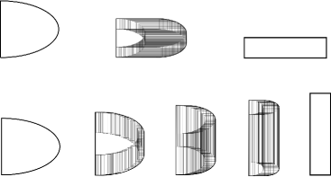
Figure 6. The convex body $\frac{1}{2}\alpha^{-1}K+\frac{1}{2}K_{2}$ (middle of the upper line) is not the image by a rotation and a translation of $(1-t)\alpha^{-1}K+tR_{\frac{\pi}{2}}(K_{2})$ (represented on the bottom line for $t=0,\frac{1}{4},\frac{1}{2},\frac{3}{4},1$).

Since $R_{\pi}[K_{2}]=[K_{2}]$, to compute the minimum this is sufficient to consider $\theta\in[-\frac{\pi}{2},\frac{\pi}{2}]$. Moreover, let $T$ be the symmetry with respect to the $x$ axis: we have $T[K_{1}]=[K_{1}]$, hence we have

$$d_{\mathscr{H}^{2}}([K_{1}],R_{\theta}[K_{2}])=d_{\mathscr{H}^{2}}(T[K_{1}],R_{\theta}[K_{2}])=d_{\mathscr{H}^{2}}([K_{1}],T\circ R_{\theta}[K_{2}])=d_{\mathscr{H}^{2}}([K_{1}],R_{-\theta}[K_{2}])~{}.$$

This shows that in fact we need only to consider $\theta\in[0,\frac{\pi}{2}]$.

Let $k_{2}^{\theta}$ be the support function of $R_{\theta}[K_{2}]$, that is $k_{2}^{\theta}(s)=k_{2}(s-\theta)$. We have

$$\cosh(d_{\mathscr{H}^{2}}([K_{1}],R_{\theta}[K_{2}]))=\frac{V_{2}(k_{1},k_{2}^{\theta})}{\sqrt{V_{2}(k_{1})V_{2}(k_{2}^{\theta})}}=\frac{f(\theta)}{2\sqrt{V_{2}(k_{1})V_{2}(k_{2})}}~{},$$

where we denote by $f(\theta)$ the function defined by

$$f(\theta)=\int_{0}^{2\pi}(k_{1}(s)k_{2}(s-\theta)-k_{1}^{\prime}(s)k_{2}^{\prime}(s-\theta))\mbox{d}s~{}.$$

Proposition 3.2 is a direct consequence of the following lemma.

Lemma 3.4.

On $[0,\frac{\pi}{2}]$, $f$ attains its minimum at the points $\theta=0$ and $\theta=\frac{\pi}{2}$.

Proof.

Fix $\theta\in(0,\frac{\pi}{2})$, and consider the function $s\mapsto k_{1}(s)k_{2}^{\prime}(s-\theta)$. This function is piecewise $\mathcal{C}^{1}$, but is not continuous: the function $k_{2}^{\prime}(s-\theta)$ has jumps, with height $\frac{1}{5}$ at the points $s=\theta$ and $s=\pi+\theta$, and with height $\frac{4}{5}$ at the points $s=\frac{\pi}{2}+\theta$ and $s=\frac{3\pi}{2}+\theta$. Hence we have

$$\int_{0}^{2\pi}(k_{1}(s)k_{2}^{\prime}(s-\theta))^{\prime}\mbox{d}s=-\frac{1}{5}k_{1}(\theta)-\frac{1}{5}k_{1}(\pi+\theta)-\frac{4}{5}k_{1}(\frac{\pi}{2}+\theta)-\frac{4}{5}k_{1}(\frac{3\pi}{2}+\theta)$$

$$=-\frac{1}{5\alpha}\sqrt{2\cos^{2}\theta+\frac{1}{2}\sin^{2}\theta}-\frac{4}{5\alpha}\sqrt{2\sin^{2}\theta+\frac{1}{2}\cos^{2}\theta}-\frac{1}{5\sqrt{2}\alpha}\sin\theta-\frac{4}{5\sqrt{2}\alpha}\cos\theta~{}.$$

The equality $(k_{1}k^{\prime}_{2})^{\prime}=k_{1}^{\prime}k_{2}^{\prime}+k_{1}k_{2}^{\prime\prime}$ gives $-k_{1}^{\prime}k_{2}^{\prime}=k_{1}k_{2}^{\prime\prime}-(k_{1}k_{2}^{\prime})^{\prime}$, so

$$-\int_{0}^{2\pi}k_{1}^{\prime}(s)k_{2}^{\prime}(s-\theta)\mbox{d}s=\int_{0}^{2\pi}(k_{1}(s)k_{2}^{\prime\prime}(s-\theta)-(k_{1}(s)k_{2}^{\prime}(s-\theta))^{\prime})\mbox{d}s~{},$$

and since $k_{2}(s-\theta)+k_{2}^{\prime\prime}(s-\theta)=0$ for almost every $s\in[0,2\pi]$ we finally obtain

$$f(\theta) = \int_{0}^{2\pi}(k_{1}(s)k_{2}(s-\theta)-k_{1}^{\prime}(s)k_{2}^{\prime}(s-\theta))\mbox{d}s$$

$$= \int_{0}^{2\pi}(k_{1}(s)(k_{2}(s-\theta)+k_{2}^{\prime\prime}(s-\theta))-(k_{1}(s)k_{2}^{\prime}(s-\theta))^{\prime})\mbox{d}s$$

$$= \frac{1}{5\alpha}\sqrt{2\cos^{2}\theta+\frac{1}{2}\sin^{2}\theta}+\frac{4}{5\alpha}\sqrt{2\sin^{2}\theta+\frac{1}{2}\cos^{2}\theta}+\frac{1}{5\sqrt{2}\alpha}\sin\theta+\frac{4}{5\sqrt{2}\alpha}\cos\theta~{}.$$

We easily check that $f(0)=f(\frac{\pi}{2})=\frac{\sqrt{2}}{\alpha}$ (the parameters of the ellipse and the segment have been chosen so that this property holds). And a direct computation shows that $f^{\prime}(0)=\frac{1}{5\sqrt{2}\alpha}>0$ and $f^{\prime}(\frac{\pi}{2})=-\frac{4}{5\sqrt{2}\alpha}<0$. Moreover, let $g:[0,1]\rightarrow[0,\infty)$ be defined by

$$g(u)=\frac{1}{5\alpha}\sqrt{\frac{3}{2}u+\frac{1}{2}}+\frac{4}{5\alpha}\sqrt{2-\frac{3}{2}u}+\frac{1}{5\sqrt{2}\alpha}\sqrt{1-u}+\frac{4}{5\sqrt{2}\alpha}\sqrt{u}~{}.$$

With the identity $\cos^{2}+\sin^{2}=1$, we easily check that $g(\cos^{2}\theta)=f(\theta)$ for any $\theta\in[0,\frac{\pi}{2}]$. Hence $f^{\prime}(\theta)=-2g^{\prime}(\cos^{2}\theta)\sin\theta\cos\theta$. But $g$ is strictly concave, hence $g^{\prime}$ has at most one zero on $[0,1]$, hence $f^{\prime}$ has also at most one zero on $(0,\frac{\pi}{2})$. And this ends the proof: if the minimum of $f$ on $[0,\frac{\pi}{2}]$ was attained at a point $\theta\notin\{0,\frac{\pi}{2}\}$, since $f^{\prime}(0)>0$ and $f^{\prime}(\frac{\pi}{2})<0$, $f^{\prime}$ would have at least 3 zeros on $(0,\frac{\pi}{2})$, and that is impossible. ∎

3.3. Embedding of hyperbolic planes

Trivially, for any $\Phi\in O(n)$ we have $\Phi[B^{n}]=[B^{n}]$. Apart from the fact that the action of $O(n)$ on $\mathscr{H}\emph{om}^{n*}$ is not proper, this says that for any $[K]\in\mathscr{H}\emph{om}^{n*}$,

(3.2) $$d_{\mathscr{S}^{n}}(\llbracket K\rrbracket,\llbracket B^{n}\rrbracket)=d_{\mathscr{H}^{n}}([K],[B^{n}])~{}.$$

From this we first deduce the following fact.

Fact 3.5 (Uniqueness of shortest paths starting from $B^{n}$).

Let $\llbracket K\rrbracket\in\mathscr{S}\emph{hape}^{n*}$. Then there is a unique shortest path from $\llbracket B^{n}\rrbracket$ to $\llbracket K\rrbracket$, which is the projection of the shortest path in $\mathscr{H}\emph{om}^{n*}$ between $[B^{n}]$ and $[K]$.

Proof.

Let $\bar{\delta}:[0,d_{\mathscr{S}^{n}}(\llbracket B^{n}\rrbracket,\llbracket K\rrbracket)]\rightarrow\mathscr{S}\emph{hape}^{n*}$ be an arc-length parametrized shortest path between $\llbracket B^{n}\rrbracket$ and $\llbracket K\rrbracket$, and let $[\delta(t)]\in\mathscr{H}\emph{om}^{n*}$ be such that $\bar{\delta}(t)=\llbracket\delta(t)\rrbracket$. Let $t\mapsto[\gamma(t)]$ be the (unique) arc-length parametrized shortest path in $\mathscr{H}\emph{om}^{n*}$ between $[B^{n}]$ and $[K]$: we want to show that $\llbracket\delta(t)\rrbracket=\llbracket\gamma(t)\rrbracket$.

For any $t\in[0,d_{\mathscr{S}^{n}}(\llbracket B^{n}\rrbracket,\llbracket K\rrbracket)]$, let $\Phi_{t}\in O(n)$ be such that

$$d_{\mathscr{S}^{n}}(\llbracket K\rrbracket,\llbracket\delta(t)\rrbracket)=d_{\mathscr{H}^{n}}([K],\Phi_{t}[\delta(t)])~{}.$$

Since $t\mapsto\llbracket\delta(t)\rrbracket$ is a geodesic in $\mathscr{S}\emph{hape}^{n*}$, we have

$$d_{\mathscr{H}^{n}}([B^{n}],\Phi_{t}[\delta(t)])+d_{\mathscr{H}^{n}}(\Phi_{t}[\delta(t)],[K]) = d_{\mathscr{S}^{n}}(\llbracket B^{n}\rrbracket,\llbracket\delta(t)\rrbracket)+d_{\mathscr{S}^{n}}(\llbracket\delta(t)\rrbracket,\llbracket K\rrbracket)$$

$$= d_{\mathscr{S}^{n}}(\llbracket B^{n}\rrbracket,\llbracket K\rrbracket)=d_{\mathscr{H}^{n}}([B^{n}],[K])~{}.$$

Hence $\Phi_{t}[\delta(t)]$ is on the shortest path between $[B^{n}]$ and $[K]$ in $\mathscr{H}\emph{om}^{n*}$. Moreover, we have $d_{\mathscr{H}^{n}}([B^{n}],\Phi_{t}[\delta(t)])=d_{\mathscr{S}^{n}}(\llbracket B^{n}\rrbracket,\llbracket\delta(t)\rrbracket)=t$ (the geodesic $t\mapsto\llbracket\delta(t)\rrbracket$ is arc-length parametrized), so $\Phi_{t}[\delta(t)]=[\gamma(t)]$ (remember that the geodesic $t\mapsto[\gamma(t)]$ is also arc-length parametrized). Finally this gives $\llbracket\delta(t)\rrbracket=\llbracket\gamma(t)\rrbracket$. ∎

In turn, we can construct totally geodesic hyperbolic surfaces in $\mathscr{S}\emph{hape}^{n*}$. Interestingly, many properties in this section are very general, but this one uses Alexandrov–Fenchel Inequality.

Proposition 3.6.

Let $\llbracket P\rrbracket,\llbracket Q\rrbracket\in\mathscr{S}\emph{hape}^{n*}$ be such that $\llbracket P\rrbracket,\llbracket Q\rrbracket$ and $\llbracket B^{n}\rrbracket$ are three different points. Let $A\in O(n)$ be such that $d_{\mathscr{S}^{n}}(\llbracket P\rrbracket,\llbracket Q\rrbracket)=d_{\mathscr{H}^{n}}([P],A[Q])$. Then the projection $\mathscr{H}\emph{om}^{n*}\rightarrow\mathscr{S}\emph{hape}^{n*}$, when restricted to the (plain) geodesic triangle with vertices $[B^{n}],[P]$ and $A[Q]$, is an isometry onto its image.

Proof.

Without loss of generality, we may assume that $A$ is the identity (that is, $d_{\mathscr{S}^{n}}(\llbracket P\rrbracket,\llbracket Q\rrbracket)=d_{\mathscr{H}^{n}}([P],[Q])$). Let $[K_{1}]$ and $[K_{2}]$ be in the geodesic triangle with vertices $[B^{n}],[P]$ and $[Q]$: since geodesics in $\mathscr{H}\emph{om}^{n*}$ are convex combinations, we can write

$$[K_{1}]=[\alpha_{1}B^{n}+\beta_{1}P+\gamma_{1}Q]\mbox{ and }[K_{2}]=[\alpha_{2}B^{n}+\beta_{2}P+\gamma_{2}Q]~{},$$

where the $\alpha_{i},\beta_{i},\gamma_{i}$ are non-negative real numbers, with $\alpha_{1}+\beta_{1}+\gamma_{1}=\alpha_{2}+\beta_{2}+\gamma_{2}=1$. We want to prove that $d_{\mathscr{S}^{n}}(\llbracket K_{1}\rrbracket,\llbracket K_{2}\rrbracket)=d_{\mathscr{H}^{n}}([K_{1}],[K_{2}])$, which means that for any $\Phi\in O(n)$ we have $d_{\mathscr{H}^{n}}([K_{1}],[K_{2}])\leq d_{\mathscr{H}^{n}}([K_{1}],\Phi[K_{2}])$. Since $V_{2}$ is $O(n)-$invariant, we only need to show that

(3.3) $$V_{2}(K_{1},K_{2})\leq V_{2}(K_{1},\Phi(K_{2}))$$

($K_{1}$ and $K_{2}$ denote two convex bodies in the equivalent classes $[K_{1}]$ and $[K_{2}]$). We have

$$V_{2}(K_{1},K_{2})=\alpha_{1}\alpha_{2}V_{2}(B^{n})+\alpha_{1}\beta_{2}V_{2}(B^{n},P)+\alpha_{1}\gamma_{2}V_{2}(B^{n},Q)$$

$$+\beta_{1}\alpha_{2}V_{2}(P,B^{n})+\beta_{1}\beta_{2}V_{2}(P)+\beta_{1}\gamma_{2}V_{2}(P,Q)$$

$$+\gamma_{1}\alpha_{2}V_{2}(Q,B^{n})+\gamma_{1}\beta_{2}V_{2}(Q,P)+\gamma_{1}\gamma_{2}V_{2}(Q)~{}.$$

Moreover $\Phi(K_{2})=\alpha_{2}B^{n}+\beta_{2}\Phi(P)+\gamma_{2}\Phi(Q)$, hence

$$V_{2}(K_{1},\Phi(K_{2}))=\alpha_{1}\alpha_{2}V_{2}(B^{n})+\alpha_{1}\beta_{2}V_{2}(B^{n},\Phi(P))+\alpha_{1}\gamma_{2}V_{2}(B^{n},\Phi(Q))$$

$$+\beta_{1}\alpha_{2}V_{2}(P,B^{n})+\beta_{1}\beta_{2}V_{2}(P,\Phi(P))+\beta_{1}\gamma_{2}V_{2}(P,\Phi(Q))$$

$$+\gamma_{1}\alpha_{2}V_{2}(Q,B^{n})+\gamma_{1}\beta_{2}V_{2}(Q,\Phi(P))+\gamma_{1}\gamma_{2}V_{2}(Q,\Phi(Q))~{}.$$

And we obviously have $V_{2}(B^{n},P)=V_{2}(B^{n},\Phi(P))$ and $V_{2}(B^{n},Q)=V_{2}(B^{n},\Phi(Q))$. Moreover, Alexandrov–Fenchel Inequality (2.3) gives $V_{2}(P)=\sqrt{V_{2}(P)V_{2}(\Phi(P))}\leq V_{2}(P,\Phi(P))$, and $V_{2}(Q)=\sqrt{V_{2}(Q)V_{2}(\Phi(Q))}\leq V_{2}(Q,\Phi(Q))$. And $d_{\mathscr{S}^{n}}(\llbracket P\rrbracket,\llbracket Q\rrbracket)=d_{\mathscr{H}^{n}}([P],[Q])$ gives $V_{2}(P,Q)\leq V_{2}(P,\Phi(Q))$ and $V_{2}(Q,P)\leq V_{2}(Q,\Phi(P))$. Since all the real numbers $\alpha_{i},\beta_{i},\gamma_{i}$ are non-negative, this gives inequality (3.3).

∎

3.4. Proof of Theorem 3

Proposition 3.1 and sections 3.2 and 3.3 give part of Theorem 3. It remains to prove the assertion about the boundary of $\mathscr{S}\emph{hape}^{n*}$. It obviously contains only one point: indeed, the boundary of $\mathscr{H}\emph{om}^{n*}$ is the set of segments up to homotheties, so the boundary of $\mathscr{S}\emph{hape}^{n*}$ is the set of segments, up to translations, positive scaling and rotations of $\mathbb{R}^{n}$, and there is only one equivalence class.

4. The space of all the (oriented) shapes

This section is an opening to the study of spaces of convex bodies, considered without making distinction between dimensions. For $p\geq 0$, let us denote by $\iota_{n,p}$ the canonical isometric embedding of $\mathbb{R}^{n}$ into $\mathbb{R}^{n+p}$ which is given by $\mathbb{R}^{n}\simeq\mathbb{R}^{n}\times\{0\}^{p}\subset\mathbb{R}^{n+p}$. Due to the intrinsic nature of $V_{2}$, we have that the map

$$\iota_{n,p}:(\mathscr{H}\emph{om}^{n*},d_{\mathscr{H}^{n}})\to(\mathscr{H}\emph{om}^{(n+p)*},d_{\mathscr{H}^{n+p}})$$

defined by $\iota_{n,p}([K])=[\iota_{n,p}(K)]$ is an isometry. Let $\mathscr{H}\emph{om}^{\infty*}$ be the union over $n$ of $\mathscr{H}\emph{om}^{n*}$, quotiented by the following equivalence relation: $[K_{1}]$ is equivalent to $[K_{2}]$ if and only if there exist $i,j\leq p$ such that $K_{1}\subset\mathbb{R}^{i}$, $K_{2}\subset\mathbb{R}^{j}$ and $[\iota_{i,p-i}(K_{1})]=[\iota_{j,p-j}(K_{2})]$. We will denote by $[K]_{\infty}$ an element of $\mathscr{H}\emph{om}^{\infty*}$. For two representatives of $[K_{1}]_{\infty},[K_{2}]_{\infty}\in\mathscr{H}\emph{om}^{\infty*}$ in $\mathbb{R}^{n}$, let us define

$$d_{\mathscr{H}^{\infty}}([K_{1}]_{\infty},[K_{2}]_{\infty})=d_{\mathscr{H}^{n}}([K_{1}],[K_{2}])~{}.$$

It is easy to see that $d_{\mathscr{H}^{\infty}}$ is well-defined and that it is actually a distance on $\mathscr{H}\emph{om}^{\infty*}$. The isometric embeddings $\iota_{n,p}$ induce isometric maps from $(\mathscr{S}\emph{hape}^{n*},d_{\mathscr{S}^{n}})$ to $(\mathscr{S}\emph{hape}^{(n+p)*},d_{\mathscr{S}^{n+p}})$, so in the same way we can define the set $\mathscr{S}\emph{hape}^{\infty*}$ and the metric space $(\mathscr{S}\emph{hape}^{\infty*},d_{\mathscr{S}^{\infty}})$.

It follows from Theorems 1 and 3 that $(\mathscr{H}\emph{om}^{\infty*},d_{\mathscr{H}^{\infty}})$ and $(\mathscr{S}\emph{hape}^{\infty*},d_{\mathscr{S}^{\infty}})$ are geodesic metric spaces. But two facts occur:

1. it may happen that a sequence of convex bodies with non-empty interior in $\mathbb{R}^{p}$ converges to a convex body in $\mathscr{H}\emph{om}^{\infty}$ when $p$ goes to infinity. Actually, for $(\epsilon_{p})_{p}$ a sequence of real numbers such that $\sqrt{p}\epsilon_{p}\rightarrow 0$, one can check that the sequence $([\iota_{n,p}(K)+\epsilon_{p}B^{n+p}]_{\infty})_{p}$ converges in $\mathscr{H}\emph{om}^{\infty*}$ to $[K]_{\infty}$. In particular, there may exist other shortest paths than the convex combinations;

2. one can check that the sequence of balls $([B^{n}]_{\infty})_{n}$ (resp. $(\llbracket B^{n}\rrbracket_{\infty})_{n}$) is a diverging Cauchy sequence.

So we address the following.

Question 4.1.

Describe the completion of $(\mathscr{H}\emph{om}^{\infty*},d_{\mathscr{H}^{\infty}})$ and $(\mathscr{S}\emph{hape}^{\infty*},d_{\mathscr{S}^{\infty}})$.

References

- [1] A. D. Alexandrov. Convex polyhedra. Springer Monographs in Mathematics. Springer-Verlag, Berlin, 2005. Translated from the 1950 Russian edition by N. S. Dairbekov, S. S. Kutateladze and A. B. Sossinsky, With comments and bibliography by V. A. Zalgaller and appendices by L. A. Shor and Yu. A. Volkov.
- [2] C. Bavard and E. Ghys. Polygones du plan et polyèdres hyperboliques. Geom. Dedicata, 43(2):207–224, 1992.
- [3] I. Belegradek. The Gromov-Hausdorff hyperspace of nonnegatively curved -spheres. Proc. Amer. Math. Soc., 146(4):1757–1764, 2018.
- [4] G. Bianchi, A. Colesanti, and C. Pucci. On the second differentiability of convex surfaces. Geom. Dedicata, 60(1):39–48, 1996.
- [5] M. R. Bridson and A. Haefliger. Metric spaces of non-positive curvature, volume 319 of Grundlehren der Mathematischen Wissenschaften [Fundamental Principles of Mathematical Sciences]. Springer-Verlag, Berlin, 1999.
- [6] D. Burago, Y. Burago, and S. Ivanov. A course in metric geometry. Providence, RI: American Mathematical Society (AMS), 2001.
- [7] F. Fillastre. From spaces of polygons to spaces of polyhedra following Bavard, Ghys and Thurston. Enseign. Math. (2), 57(1-2):23–56, 2011.
- [8] F. Fillastre and I. Izmestiev. A remark on spaces of flat metrics with cone singularities of constant sign curvatures. In Séminaire de théorie spectrale et géométrie (2016-2017), Tome 34, pages 65–92. Grenoble.
- [9] F. Fillastre and I. Izmestiev. Shapes of polyhedra, mixed volumes and hyperbolic geometry. Mathematika, 63(1):124–183, 2017.
- [10] H. Groemer. Geometric applications of Fourier series and spherical harmonics, volume 61 of Encyclopedia of Mathematics and its Applications. Cambridge University Press, Cambridge, 1996.
- [11] E. Heil. Extensions of an inequality of Bonnesen to -dimensional space and curvature conditions for convex bodies. Aequationes Math., 34(1):35–60, 1987.
- [12] R. Langevin, G. Levitt, and H. Rosenberg. Hérissons et multihérissons (enveloppes parametrées par leur application de Gauss). In Singularities (Warsaw, 1985), volume 20 of Banach Center Publ., pages 245–253. PWN, Warsaw, 1988.
- [13] Y. Martinez-Maure. Hedgehogs and area of order . Arch. Math. (Basel), 67(2):156–163, 1996.
- [14] Y. Martinez-Maure. De nouvelles inégalités géométriques pour les hérissons. Arch. Math. (Basel), 72(6):444–453, 1999.
- [15] Y. Martinez-Maure. Geometric inequalities for plane hedgehogs. Demonstratio Math., 32(1):177–183, 1999.
- [16] Y. Martinez-Maure. Geometric study of Minkowski differences of plane convex bodies. Canad. J. Math., 58(3):600–624, 2006.
- [17] V. S. Matveev. Does positively curved sphere admit an isometric embedding as hypersurface in euclidean space? MathOverflow. https://mathoverflow.net/q/143945 (version: 2013-10-04).
- [18] N. Monod and P. Py. An exotic deformation of the hyperbolic space. Amer. J. Math., 136(5):1249–1299, 2014.
- [19] V. Oliker. Generalized convex bodies and generalized envelopes. In Geometric analysis (Philadelphia, PA, 1991), volume 140 of Contemp. Math., pages 105–113. Amer. Math. Soc., Providence, RI, 1992.
- [20] R. Schneider. Convex bodies: the Brunn-Minkowski theory, volume 151 of Encyclopedia of Mathematics and its Applications. Cambridge University Press, Cambridge, expanded edition, 2014.
- [21] R. Schneider. The typical irregularity of virtual convex bodies. J. Convex Anal., 25(1):103–118, 2018.
- [22] W. P. Thurston. Shapes of polyhedra and triangulations of the sphere. In The Epstein birthday schrift, volume 1 of Geom. Topol. Monogr., pages 511–549. Geom. Topol. Publ., Coventry, 1998.
- [23] R. A. Vitale. metrics for compact, convex sets. J. Approx. Theory, 45(3):280–287, 1985.