Statistics of photon-subtracted and photon-added states

Abstract

The subtraction or addition of a prescribed number of photons to a field mode does not, in general, simply shift the probability distribution by the number of subtracted or added photons. Subtraction of a photon from an initial coherent state, for example, leaves the photon statistics unchanged and the same process applied to an initial thermal state increases the mean photon number. We present a detailed analysis of the effects of the initial photon statistics on those of the state from which the photons have been subtracted or to which they have been added. Our approach is based on two closely-related moment generating functions, one well-established and one that we introduce.

I Introduction

The addition or subtraction of a single photon from the radiation field is the most fundamental process by which matter interacts with light. The ability to achieve this level of control in experiments has been used to produce novel non-classical states of light by the process of “degaussification” Philippe and in a direct demonstration of the commutation relation between the annihilation and creation operators Bellini1 ; Bellini2 ; Bellini3 .

There has been considerable interest in both the processes of photon addition and subtraction and also in the properties of the quantum states produced by these processes. Indeed, a discussion of these appears in Agarwal’s textbook Girishbook . Four developments make these states worthy of further consideration. First there is the rapid advance towards practical implementation of quantum key distribution Wootters ; Assche ; QIbook and the associated eavesdropping activities including photon removal. Second is the demonstration, recently, of the effects of photon subtraction on the visibility of optical fringes with thermal light Bobexpt ; Lanz and, more generally, the suggestion that both photon-subtracted and photon-added states may provide advantages in metrology Treps . Third is the requirement for non-Gaussian processes (including photon subtraction or addition) in order to demonstrate the supremacy of continuous variable quantum computing Eisert ; Loock ; Douce ; Walschaers . Finally, and perhaps most intriguing, is the demonstration that photon subtraction from a thermal pulse results in an increase in the energy and that this information can be used for the extraction of work Demon .

There have been a number of earlier studies of photon-added, and particularly of photon-subtracted states. Interest in these states appears to originate with the work of Agarwal and Tara Tara ; AgarwalNeg . Implementing this technique has been shown to introduce novel quantum effects including the generation of novel superposition states Jeong ; Ourjoumtsev ; Neergaard ; Biswas . More recently, attention has turned to the results of multiple addition and subtraction events and how these might be used to engineer the properties of the light Fiurasek ; Bogdanov .

We note that uncontrolled photon subtraction events arise in the quantum jumps approach to dissipation Carmichael1 ; Dalibard ; Gardiner ; Carmichael2 and these have been shown to have a dramatic effect, in particular, on non-classical phenomena including Schrödinger-cat states Garraway and on revivals in the Jaynes-Cummings model JCM1 ; JCM2 . Here, however, our focus will be on processes designed to subtract or add a given number of photons even though the probability for the process to be successful will typically be small.

In this paper we aim to give a thorough description of the photon statistics of photon-added and photon-subtracted states. Our preferred tools for this are the moment generating function, as advocated by Bogdanov et al Bogdanov , and a closely related function which we introduce. We find that a combination of these allows us to make very general statements about the effects of subtracting or adding a given number of photons and also about the relationships between these two processes.

II Photon-added and photon-subtracted states

We shall be concerned, for simplicity, solely with states of a single quantised field mode and the effect of successfully either subtracting or adding one or more photons to the state of the field. We denote by $\hat{\rho}^{0}$ the initial state of the field mode and then the subtraction or addition of a single photon will produce a state with density operator

$$\hat{\rho}^{1-} = \frac{\hat{a}\hat{\rho}^{0}\hat{a}^{\dagger}}{{\rm Tr}(\hat{\rho}^{0}\hat{a}^{\dagger}\hat{a})}$$

$$\hat{\rho}^{1+} = \frac{\hat{a}^{\dagger}\hat{\rho}^{0}\hat{a}}{{\rm Tr}(\hat{\rho}^{0}\hat{a}\hat{a}^{\dagger})},$$ (1)

respectively. Adding or subtracting more than a single photon in this way is challenging, experimentally, but it is, nevertheless, interesting to consider this possibility at least theoretically, principally for the insights into the nature of the statistics, to consider states in which more than a single photon is subtracted or added. We denote the states following the subtraction or addition of $\ell$ photons as

$$\hat{\rho}^{\ell-} = \frac{\hat{a}^{\ell}\hat{\rho}^{0}\hat{a}^{\dagger\ell}}{{\rm Tr}(\hat{\rho}^{0}\hat{a}^{\dagger\ell}\hat{a}^{\ell})}$$

$$\hat{\rho}^{\ell+} = \frac{\hat{a}^{\dagger\ell}\hat{\rho}^{0}\hat{a}^{\ell}}{{\rm Tr}(\hat{\rho}^{0}\hat{a}^{\ell}\hat{a}^{\dagger\ell})}.$$ (2)

That these photon-added states, in particular, are worthy of further consideration was suggested many years ago by Agarwal and Tara Tara .

We note that producing photon-subtracted or photon-added states of the form under consideration is necessarily a probabilistic process with, typically, a low probability of success. There are processes that remove a photon with certainty, if at least one photon is present Calsamiglia ; Oi ; Rosenblum , but these are more difficult to implement than the probabilistic processes and will not concern us here. The simplest way to either subtract or add a single photon is by a weak interaction with an ancillary mode, with the detection of a photon in this additional mode heralding a successful subtraction or addition event Girishbook . For completeness, we summarise briefly these two processes. To realise photon subtraction we combine our mode, $\hat{a}$, with a second one, $\hat{b}$, prepared in its vacuum state, using a weakly-reflecting beam splitter as depicted in Fig. 1(a). We can describe the action of the beam splitter by a unitary transformation coupling the two modes Methods :

$$\hat{U}=\exp\left[i\theta(\hat{a}^{\dagger}\hat{b}+\hat{b}^{\dagger}\hat{a})\right].$$ (3)

The action of this on the two input modes produces the state

$$\hat{U}\hat{\rho}^{0}\otimes|0\rangle\langle 0|\hat{U}^{\dagger}\approx(1+i\theta\hat{b}^{\dagger}\hat{a})\hat{\rho}^{0}\otimes|0\rangle\langle 0|(1-i\theta\hat{a}^{\dagger}\hat{b}).$$ (4)

If we detect a photon in the output $b$ mode then the output $a$ mode conditioned on this detection will be the photon-subtracted state $\hat{\rho}^{1-}$. To realise photon addition we proceed in the same way but utilise a weak nonlinear optical parametric-amplfication process, as depicted in Fig. 1(b), rather than a beam splitter. We can describe this process by a unitary transformation of the form Methods

$$\hat{U}=\exp\left[i\vartheta(\hat{a}^{\dagger}\hat{b}^{\dagger}+\hat{b}\hat{a})\right].$$ (5)

The action of this on the two input modes, with mode $b$ again prepared in the vacuum state, produces the two-mode output state

$$\hat{U}\hat{\rho}^{0}\otimes|0\rangle\langle 0|\hat{U}^{\dagger}\approx(1+i\vartheta\hat{a}^{\dagger}\hat{b}^{\dagger})\hat{\rho}^{0}\otimes|0\rangle\langle 0|(1-i\vartheta\hat{b}\hat{a}).$$ (6)

As with the photon-subtraction process, if we detect a photon in the output $b$ mode then the output $a$ mode conditioned on this detection will be the photon-added state $\hat{\rho}^{1+}$. We can produce, at least in principle, multiple photon-subtracted or photon-added states by combining a number of single-photon subtraction or addition events accepting, of course, the fact that the probability for successfully adding or subtracting the photons falls off rapidly as the number of subtraction or addition events increases.

Figure 1: Schematic for implementations of (a) photon subtraction using a weakly reflecting beam splitter and (b) photon addition using a weak parametric amplifier.

We present in this paper a detailed study of the statistics of photon-subtracted and photon-added states and provide a simple and efficient way of obtaining these by expressing the properties of these states in terms of those of the preprocessed state $\hat{\rho}^{0}$. As a foretaste of this we prove two simple properties. The first of these is the well-known fact that subtracting a single photon can result in an increase in the mean photon number Ueda ; Ban ; Zavatta ; Dodonov and there is a simple and general criterion for this to occur. The second is that adding a single photon results in the mean photon number increasing by at least one. The mean photon number for the photon-subtracted state is Bogdanov

$$\langle\hat{n}\rangle^{1-}=\frac{{\rm Tr}(\hat{\rho}^{0}\hat{a}^{\dagger 2}\hat{a}^{2})}{{\rm Tr}(\hat{\rho}^{0}\hat{a}^{\dagger}\hat{a})}.$$ (7)

This will be greater than the mean photon number for the original state, ${\rm Tr}(\hat{\rho}^{0}\hat{a}^{\dagger}\hat{a})$, if the second-order coherence function for $\hat{\rho}^{0}$

$$g^{(2)}=\frac{{\rm Tr}(\hat{\rho}^{0}\hat{a}^{\dagger 2}\hat{a}^{2})}{[{\rm Tr}(\hat{\rho}^{0}\hat{a}^{\dagger}\hat{a})]^{2}}$$ (8)

is greater than unity, corresponding to a super-Poissonian state, one with a photon-number variance exceeding the mean value: $\Delta n^{2}>\langle\hat{n}\rangle$ Demon ; Ueda ; Zavatta . For the photon-added state the mean value of the photon number is

$$\langle\hat{n}\rangle^{1+} = \frac{{\rm Tr}(\hat{\rho}^{0}\hat{a}\hat{a}^{\dagger}\hat{a}\hat{a}^{\dagger})}{{\rm Tr}(\hat{\rho}^{0}\hat{a}\hat{a}^{\dagger})}$$ (9)

$$= \frac{{\rm Tr}[\hat{\rho}^{0}(\hat{n}+1)^{2}]}{{\rm Tr}[\hat{\rho}^{0}(\hat{n}+1)]}.$$

As the mean square of a quantity (in this case $\hat{n}+1$) is greater than or equal to the square of the mean it necessarily follows that photon addition will increase the mean photon number by at least one: $\langle\hat{n}\rangle^{1+}\geq\langle\hat{n}\rangle^{0}+1$.

III Moment generating functions

Our aim is to determine, in a general manner and as simply as possible, the relationship between the photon statistics of the initial state, with density operator $\hat{\rho}^{0}$, and that of a state following the subtraction or addition of a given number of photons. The most natural tool to use for this is a moment generating function, as is so often the case in statistics Jeffreys ; Lukacs ; Helstrom ; Renyi ; vanKampen ; GardinerStoch ; Grimmett . We shall employ a pair of closely related moment generating functions:

$$\mathcal{M}(\mu) = \sum_{n=0}^{\infty}(1-\mu)^{n}P(n)$$

$$\mathcal{N}(\lambda) = \sum_{n=0}^{\infty}(1+\lambda)^{-(n+1)}P(n),$$ (10)

where $P(n)$ is the probabililty that $n$ photons are present. The first of these is the familiar quantity introduced into quantum optics by Glauber (and denoted by him as $Q(s)$) Glauber ; JakemanPike . The second, although clearly simply related to the first is, to the best of our knowledge, new to quantum optics and is introduced here because of its use in treating photon-added states. Some of the properties of these functions are reviewed in Appendix A. The main properties of these that we shall exploit are that $\mathcal{M}(\mu)$ and $\mathcal{N}(\lambda)$ give, resepctively, the factorial moments, $\langle\hat{n}^{(m)}\rangle=\langle\hat{n}(\hat{n}-1)\cdots(\hat{n}-m+1)\rangle$, and the negative factorial moments, $\langle(\hat{n}+1)^{(-m)}\rangle=\langle(\hat{n}+1)(\hat{n}+2)\cdots(\hat{n}+m)\rangle$, simply by differentiation:

$$\langle\hat{n}^{(m)}\rangle = \left.\left(-\frac{d}{d\mu}\right)^{m}\mathcal{M}(\mu)\right|_{\mu=0}$$

$$\langle(\hat{n}+1)^{(-m)}\rangle = \left.\left(-\frac{d}{d\lambda}\right)^{m}\mathcal{N}(\lambda)\right|_{\lambda=0},$$ (11)

and that both functions give, straightforwardly, the probability that the photon number is even or odd Methods :

$$\mathcal{M}(2)=P({\rm even})-P({\rm odd})=-\mathcal{N}(-2).$$ (12)

An important feature of the moment generating functions is the comparative ease with which we can find these quantities for important quantum states of light. We illustrate this point by presenting these for five commonly used types of state: the number (or Fock) states, the coherent states, the thermal or chaotic states, the squeezed vacuum states and finally the Schrödinger cat states. For the photon-number state $|N\rangle$ the probability distribution is simply $P(n)=\delta_{n,N}$ and we have

$$\mathcal{M}_{|N\rangle}(\mu) = (1-\mu)^{N}$$

$$\mathcal{N}_{|N\rangle}(\lambda) = (1+\lambda)^{-(N+1)}.$$ (13)

The coherent states, $|\alpha\rangle$, have a Poissonian photon number probability distribution Methods ; Rodney , $P(n)=e^{-|\alpha|^{2}}|\alpha|^{2n}/n!$, and the moment generating functions are

$$\mathcal{M}_{|\alpha\rangle}(\mu) = e^{-\mu|\alpha|^{2}}$$

$$\mathcal{N}_{|\alpha\rangle}(\lambda) = \frac{1}{1+\lambda}\exp\left(-\frac{\lambda|\alpha|^{2}}{1+\lambda}\right).$$ (14)

It is straightforward to use these to calculate the factorial moments from the moment generating functions using (III). For the positive moments we find the familiar form Methods ; Rodney

$$\langle\hat{n}^{(m)}\rangle_{|\alpha\rangle}=|\alpha|^{2m}.$$ (15)

The negative moments have a more complicated form and we give, here, only the first two of these:

$$\langle(\hat{n}+1)^{(-1)}\rangle_{|\alpha\rangle} = |\alpha|^{2}+1$$

$$\langle(\hat{n}+1)^{(-2)}\rangle_{|\alpha\rangle} = |\alpha|^{4}+4|\alpha|^{2}+2.$$ (16)

Higher order moments are readily obtained by further differentiation of $\mathcal{N}_{|\alpha\rangle}(\lambda)$. The moment generating function shows, also, that all coherent states have a greater probability that the photon number is even than that it is odd as $\mathcal{M}(2)=-\mathcal{N}(-2)=e^{-2|\alpha|^{2}}$.

The thermal state is mixed with a density operator that is diagonal in the number-state basis. The probability that there are $n$ photons has the familiar Bose-Einstein form, $P(n)=\bar{n}^{n}/(\bar{n}+1)^{n+1}$, where $\bar{n}$ is the mean photon number. For this state the moment generating functions are

$$\mathcal{M}_{\rm th}(\mu) = \frac{1}{1+\mu\bar{n}}$$

$$\mathcal{N}_{\rm th}(\lambda) = \frac{1}{1+\lambda(\bar{n}+1)}.$$ (17)

The positive and negative moments for the thermal state, derived from these moment generating functions, have the simple forms:

$$\langle\hat{n}^{(m)}\rangle_{\rm th} = m!\bar{n}^{m}$$

$$\langle(\hat{n}+1)^{(-m)}\rangle_{\rm th} = m!(\bar{n}+1)^{m}.$$ (18)

Like the coherent states, all thermal states have a higher probability that the photon number is even than that it is odd: $\mathcal{M}(2)=-\mathcal{N}(-2)=(1+2\bar{n})^{-1}$.

A much-studied and important non-classical state is the squeezed vacuum, $|\zeta\rangle$, which is a superposition of only even photon-number states Methods ; Rodney :

$$P_{|\zeta\rangle}(2n) = \frac{1}{\sqrt{\bar{n}+1}}\left(\frac{\bar{n}}{\bar{n}+1}\right)^{n}\frac{(2n)!}{2^{2n}(n!)^{2}}$$

$$P_{|\zeta\rangle}(2n+1) = 0,$$ (19)

where $\bar{n}$ is the mean photon number. For this state the moment generating functions are

$$\mathcal{M}_{|\zeta\rangle}(\mu) = (1+2\mu\bar{n}-\mu^{2}\bar{n})^{-1/2}$$

$$\mathcal{N}_{|\zeta\rangle}(\lambda) = \frac{1}{1+\lambda}\left(1+\frac{\lambda(2+\lambda)}{(1+\lambda)^{2}}\bar{n}\right)^{-1/2}.$$ (20)

Note that for this state $\mathcal{M}(2)=1=-\mathcal{N}(-2)$, which reflects the fact that the photon number is even. For the squeezed vacuum state the first two positive and negative factorial moments, calculated from the moment generating function, are

$$\langle\hat{n}^{(1)}\rangle = \bar{n}$$

$$\langle\hat{n}^{(2)}\rangle = 3\bar{n}^{2}+\bar{n}$$

$$\langle(\hat{n}+1)^{(-1)}\rangle = \bar{n}+1$$

$$\langle(\hat{n}+1)^{(-2)}\rangle = 3\bar{n}^{2}+5\bar{n}+2.$$ (21)

Our final example is the even and odd Schrödinger cat states, $|\alpha\pm\rangle$, which are superpositions of a pair of coherent states Girishbook :

$$|\alpha\pm\rangle=\frac{1}{\sqrt{2(1\pm e^{-2|\alpha|^{2}})}}\left(|\alpha\rangle\pm|-\alpha\rangle\right).$$ (22)

Among the interesting properties of these states is the fact that they are superpositions of only even photon numbers

$$P_{|\alpha+\rangle}(2n) = \frac{1}{\cosh|\alpha|^{2}}\frac{|\alpha|^{4n}}{(2n)!}$$

$$P_{|\alpha+\rangle}(2n+1) = 0\,,$$ (23)

or odd photon numbers respectively

$$P_{|\alpha-\rangle}(2n) = 0$$

$$P_{|\alpha-\rangle}(2n+1) = \frac{1}{\sinh|\alpha|^{2}}\frac{|\alpha|^{2(2n+1)}}{(2n+1)!}.$$ (24)

It is straightforward to calculate the forms of our two moment generating functions for these states. For the even Schrödinger cat state we find

$$\mathcal{M}_{|\alpha+\rangle}(\mu) = \frac{\cosh[(1-\mu)|\alpha|^{2}]}{\cosh|\alpha|^{2}}$$

$$\mathcal{N}_{|\alpha+\rangle}(\lambda) = \frac{\cosh[|\alpha|^{2}/(1+\lambda)]}{(1+\lambda)\cosh|\alpha|^{2}},$$ (25)

so that $\mathcal{M}(2)=1=-\mathcal{N}(-2)$ because the photon number is even. For the odd Schrödinger cat state, however, our moment generating functions are

$$\mathcal{M}_{|\alpha-\rangle}(\mu) = \frac{\sinh[(1-\mu)|\alpha|^{2}]}{\sinh|\alpha|^{2}}$$

$$\mathcal{N}_{|\alpha-\rangle}(\lambda) = \frac{\sinh[|\alpha|^{2}/(1+\lambda)]}{(1+\lambda)\sinh|\alpha|^{2}},$$ (26)

for which $\mathcal{M}(2)=-1=-\mathcal{N}(-2)$, which is a consequence of the fact that only odd photon numbers are present in the odd cat state. As with our other examples, it is straightforward to use the moment generating functions to obtain the positive and negative factorial moments for these states. For the even cat states we find

$$\langle\hat{n}^{(1)}\rangle_{|\alpha_{+}\rangle} = |\alpha|^{2}\tanh|\alpha|^{2}$$

$$\langle\hat{n}^{(2)}\rangle_{|\alpha_{+}\rangle} = |\alpha|^{4}$$

$$\langle(\hat{n}+1)^{(-1)}\rangle_{|\alpha_{+}\rangle} = |\alpha|^{2}\tanh|\alpha|^{2}+1$$

$$\langle(\hat{n}+1)^{(-2)}\rangle_{|\alpha_{+}\rangle} = |\alpha|^{4}+4|\alpha|^{2}\tanh|\alpha|^{2}+2.$$ (27)

The first two of these mean that the even cat state is super-Poissonian with $\Delta n^{2}>\langle\hat{n}\rangle$. For the odd cat states we have

$$\langle\hat{n}^{(1)}\rangle_{|\alpha_{+}\rangle} = |\alpha|^{2}\coth|\alpha|^{2}$$

$$\langle\hat{n}^{(2)}\rangle_{|\alpha_{+}\rangle} = |\alpha|^{4}$$

$$\langle(\hat{n}+1)^{(-1)}\rangle_{|\alpha_{+}\rangle} = |\alpha|^{2}\coth|\alpha|^{2}+1$$

$$\langle(\hat{n}+1)^{(-2)}\rangle_{|\alpha_{+}\rangle} = |\alpha|^{4}+4|\alpha|^{2}\coth|\alpha|^{2}+2.$$ (28)

We see that, in contrast with the even cat states, the odd states are sub-Poissonian with $\Delta n^{2}<\langle\hat{n}\rangle$.

IV Statistics of photon-subtracted states

The simplest way to appreciate the changes in the statistics of a photon-subtracted state is through the factorial moments. The $m^{\rm th}$ factorial moment of the photon number is defined to be

$$\langle\hat{n}^{(m)}\rangle = \langle\hat{n}(\hat{n}-1)\cdots(\hat{n}-m+1)\rangle$$ (29)

$$= \langle\hat{a}^{\dagger m}\hat{a}^{m}\rangle.$$

When written in this form it is readily apparent that the $m^{\rm th}$ factorial moment for the $\ell$-photon subtracted state is simply related to the $(m+\ell)^{\rm th}$ factorial moment of the initial, pre photon-subtraction state:

$$\langle\hat{n}^{(m)}\rangle^{\ell-} = \frac{{\rm Tr}(\hat{a}^{\dagger m}\hat{a}^{m}\hat{a}^{\ell}\hat{\rho}^{0}\hat{a}^{\dagger\ell})}{{\rm Tr}(\hat{\rho}^{0}\hat{a}^{\dagger\ell}\hat{a}^{\ell})}$$ (30)

$$= \frac{\langle\hat{n}^{(m+\ell)}\rangle^{0}}{\langle\hat{n}^{(\ell)}\rangle^{0}},$$

which is the ratio of the $(m+\ell)^{\rm th}$ and $\ell^{\rm th}$ factorial moments for the initial, pre photon-subtraction state.

It is natural and straightforward to express the full photon statistics of the photon subtracted states in terms of the moment generating function $\mathcal{M}(\mu)$. To see this we make use of the expression for the moment generating function in terms of the factorial moments, Eq. (94), to write $\mathcal{M}(\mu)$ for the $\ell$-photon subtracted state in the form

$$\mathcal{M}^{\ell-}(\mu) = \sum_{m=0}^{\infty}\frac{(-\mu)^{m}}{m!}\frac{\langle\hat{n}^{(m+\ell)}\rangle^{0}}{\langle\hat{n}^{(\ell)}\rangle^{0}}$$ (31)

$$= \frac{1}{\langle\hat{n}^{(\ell)}\rangle^{0}}\left(-\frac{d}{d\mu}\right)^{\ell}\mathcal{M}^{0}(\mu),$$

so the moment generating function for the $\ell$-photon subtracted state is simply the $\ell^{\rm th}$ derivative of that for the pre photon-subtracted state, normalised so that $\mathcal{M}^{\ell-}(0)=1$ Bogdanov .

It remains to demonstrate the utility of the simple photon-subtraction transformation of the moment generating function, which we do by exploring the effects on the states considered in the preceding section. The effect of a successful $\ell$-photon subtraction on the number state $|N\rangle$ is simply to reduce the photon number to $N-\ell$ and this is reflected in the corresponding moment generating function, which takes the form

$$\mathcal{M}_{|N\rangle}^{\ell-}(\mu)=(1-\mu)^{N-\ell},$$ (32)

which we recognise as the moment generating function for the photon number state $|N-\ell\rangle$.

The effect of photon subtraction on the coherent state is interesting; the statistics are unchanged by the process:

$$\mathcal{M}_{|\alpha\rangle}^{\ell-}(\mu)=e^{-\mu|\alpha|^{2}}=\mathcal{M}_{|\alpha\rangle}^{0}(\mu).$$ (33)

The reason for this is that the coherent state is a right-eigenstate of the annihilation operator and hence $(\hat{a})^{\ell}|\alpha\rangle=(\alpha)^{\ell}|\alpha\rangle$, so the $\ell$-photon subtracted coherent state is simply the initial coherent state. The physical origin of this unchanging character under photon subtraction is the fact that a coherent state incident on a beam-splitter produces two output modes each of which is in a coherent state, with no entanglement created between the modes. This process is depicted in Fig. 2. Here an initial coherent state is combined with a vacuum mode on a very weakly reflecting beam splitter, which enacts the state transformation $|\alpha\rangle|{\rm vac}\rangle\rightarrow|t\alpha\rangle|r\alpha\rangle\approx|\alpha\rangle|r\alpha\rangle$. There is no correlation between the two output modes and the statistics of the transmitted mode are independent of whether or not a photocount is recorded at the detector placed to detect any reflected light.

Figure 2: The action of our photon subtraction process on an initial coherent state $|\alpha\rangle$.

For the thermal states, photon subtraction has a dramatic effect on the statistics Bogdanov including the increase in the mean photon number mentioned earlier. After the successful subtraction of $\ell$ photons, an initial thermal state with mean photon number $\bar{n}$ will have the moment generating function

$$\mathcal{M}_{\rm th}^{\ell-}(\mu)=(1+\mu\bar{n})^{-(\ell+1)}=[\mathcal{M}_{\rm th}(\mu)]^{\ell+1}.$$ (34)

This means, in particular, that the mean photon number but also all of the factorial moments for the photon-subtracted thermal state exceed those for the initial thermal state:

$$\langle\hat{n}^{(m)}\rangle_{\rm th}^{\ell-} = \frac{(m+\ell)!}{\ell!}\bar{n}^{m}$$ (37)

$$= \left(\begin{array}[]{c}m+\ell\\ \ell\end{array}\right)\langle\hat{n}^{(m)}\rangle_{\rm th}^{0}.$$

To understand how this happens, we need only note that the photon subtraction process is more likely to succeed if there are more photons initially present, hence success in subtracting photons makes it a posteriori more likely that a greater number of photons were present initially. We return to this point at the end of this section.

As a final illustration, we turn to the two classes of non-classical state for which the photon number is either even or odd: the squeezed vacuum and Schrödinger cat states. For the cat states this is a very simple process - subtracting an even number of photons leaves the cat-state unchanged, but taking away an odd number of photons causes an even cat to become an odd cat and an odd cat is transformed into an even cat state:

$$\mathcal{M}_{|\alpha\pm\rangle}^{2\ell-}(\mu) = \mathcal{M}_{|\alpha\pm\rangle}(\mu)$$

$$\mathcal{M}_{|\alpha\pm\rangle}^{2\ell+1-}(\mu) = \mathcal{M}_{|\alpha\mp\rangle}(\mu).$$ (38)

The same procedure may readily be applied to the squeezed vacuum state, but the general expression for the moment generating function for the $\ell$-photon subtracted state is rather unwieldy and we give here expressions only for the subtraction of one or two photons:

$$\mathcal{M}_{|\zeta\rangle}^{1-}(\mu) = \frac{1-\mu}{(1+2\mu\bar{n}-\mu^{2}\bar{n})^{3/2}}$$

$$\mathcal{M}_{|\zeta\rangle}^{2-}(\mu) = \frac{1+\bar{n}(3-4\mu+2\mu^{2})}{(1+2\mu\bar{n}-\mu^{2}\bar{n})^{5/2}(1+3\bar{n})}.$$ (39)

We note that $\mathcal{M}_{|\zeta\rangle}^{1-}(1)=0$, corresponding to the fact that there is no vacuum component in this state and also that $\mathcal{M}_{|\zeta\rangle}^{1-}(2)=-1$ and $\mathcal{M}_{|\zeta\rangle}^{2-}(2)=1$, corresponding to states with only odd or even photon numbers, as should be the case.

IV.1 Probability of successful photon subtraction

We have seen that the process of photon subtraction has features that might seem at first to be counter-intuitive. These include the fact that the mean photon number for an initial thermal state is increased by photon subtraction and that the Poissonian statistics of a coherent state are unchanged by the process. It should be emphasised that these features alone suffice to demonstrate that the process of photon subtraction, as envisaged here, must be a probabilistic one, for were it deterministic then photon-number conservation would, necessarily, produce a reduced number of photons in the output state Calsamiglia . A simple example may help to clarify this point. Let us suppose that we have a mode prepared in a mixture (or a superposition) of the vacuum and the 10 photon state with equal prior probabilities ($P^{0}(0)=\frac{1}{2}$, $P^{0}(10)=\frac{1}{2}$). It follows that the initial mean photon number is 5. If we succeed in subtracting a photon then the resulting field mode will have a mean photon number of 9, as the fact that the photon subtraction was successful implies that there were, on this occasion, 10 photons present initially.

It is interesting to note, however, that the statistics of the photon-subtracted states allow us to make inferences, using Bayesian reasoning Box ; Mackay , concerning the probability of success in the process of photon subtraction. To demonstrate this we consider just a single simple example, the success of photon subtraction for an initial coherent state. We know that a successful single-photon subtraction leaves the photon number probability distribution for an initial coherent state unchanged and hence the probability that there are $n-1$ photons present given a successful photon subtraction is

$$P^{1-}(n-1|{\rm succ.})=e^{-|\alpha|^{2}}\frac{|\alpha|^{2(n-1)}}{(n-1)!}.$$ (40)

As there was a photon subtraction it follows, necessarily, that this is also the posterior probability that there were $n$ photons present prior to the subtraction event:

$$P^{0}(n|{\rm succ.})=e^{-|\alpha|^{2}}\frac{|\alpha|^{2(n-1)}}{(n-1)!}.$$ (41)

We can use Bayes’ theorem to obtain, from this, the probability of successfully subtracting a photon given that $n$ photons were initially present:

$$P^{0}({\rm succ.}|n)P^{0}(n) = P^{0}(n|{\rm succ.})P({\rm succ.})$$

$$\Rightarrow P^{0}({\rm succ.}|n)e^{-|\alpha|^{2}}\frac{|\alpha|^{2n}}{n!} = e^{-|\alpha|^{2}}\frac{|\alpha|^{2(n-1)}}{(n-1)!}P({\rm succ.})$$

$$\Rightarrow P^{0}({\rm succ.}|n) = n\frac{P({\rm succ.})}{|\alpha|^{2}}.$$ (42)

Hence the probability for successfully subtracting a single photon is proportional to the number of photons initially present. There is a simple reason for this, which becomes clear on referring to the physical realisation of the photon subtraction device, based on a weakly reflecting beam splitter: each photon in the input state is reflected and then detected with a small probability, $p$, thus the probability that one of the initial $n$ photons present will be so removed is $np(1-p)^{n-1}$ Methods , which, for the very small reflection probabilities considered here, is approximately $np$.

V Statistics of photon-added states

For the photon-added states it is the negative or ascending factorial moments Steffensen ,

$$\langle(\hat{n}+1)^{(-m)}\rangle = \langle(\hat{n}+1)(\hat{n}+2)\cdots(\hat{n}+m)\rangle$$ (43)

$$= \langle\hat{a}^{m}\hat{a}^{\dagger m}\rangle,$$

rather than the more familiar factorial moments that provide the natural description of the photon statistics. These negative factorial moments are the expectation values of the antinormal-ordered powers of the number operator rather than the normally-ordered moments that form the factorial moments. There is a simple relationship between the negative factorial moments for the photon-added states and those for the initial state that follows directly from the form of the states:

$$\langle(\hat{n}+1)^{(-m)}\rangle^{\ell+} = \frac{{\rm Tr}(\hat{a}^{m}\hat{a}^{\dagger m}\hat{a}^{\dagger\ell}\hat{\rho}^{0}\hat{a}^{\ell})}{{\rm Tr}(\hat{\rho}^{0}\hat{a}^{\dagger\ell}\hat{a}^{\ell})}$$ (44)

$$= \frac{\langle(\hat{n}+1)^{(-m-\ell)}\rangle^{0}}{\langle(\hat{n}+1)^{(-\ell)}\rangle^{0}},$$

which is the ratio of $(m+\ell)^{\rm th}$ and $\ell^{\rm th}$ negative factorial moments for the initial, pre photon-addition state.

For the photon-added states it is natural to use our second moment generating function, $\mathcal{N}(\lambda)$. To construct this quantity we make use of the expression, Eq. (104), for $\mathcal{N}(\lambda)$ in terms of the negative factorial moments:

$$\mathcal{N}^{\ell+}(\lambda) = \sum_{m=0}^{\infty}\frac{(-\lambda)^{m}}{m!}\frac{\langle(\hat{n}+1)^{(-m-\ell)}\rangle^{0}}{\langle(\hat{n}+1)^{(-\ell)}\rangle^{0}}$$ (45)

$$= \frac{1}{\langle(\hat{n}+1)^{(-\ell)}\rangle^{0}}\left(-\frac{d}{d\lambda}\right)^{\ell}\mathcal{N}^{0}(\lambda),$$

so the moment generating function (of the second kind) for the $\ell$-photon added state is simply the $\ell^{\rm th}$ derivative of that for the pre photon-added state, normalised so that $\mathcal{N}^{\ell+}(0)=1$.

We have seen that the process of adding a single photon increases the mean photon number by at least one. We can also arrive at this as a result of the general expression Eq. (44), by noting that

$$\langle(\hat{n}+1)^{(-1)}\rangle^{\ell+} = \langle(\hat{n}+1)\rangle^{\ell+}$$ (46)

$$= \frac{\langle(\hat{n}+1)\cdots(\hat{n}+\ell+1)\rangle^{0}}{\langle(\hat{n}+1)\cdots(\hat{n}+\ell)\rangle^{0}}$$

$$= \ell+\frac{\langle(\hat{n}+1)(\hat{n}+1)\cdots(\hat{n}+\ell)\rangle^{0}}{\langle(\hat{n}+1)\cdots(\hat{n}+\ell)\rangle^{0}}$$

$$\geq \ell+\langle(\hat{n}+1)\rangle^{0},$$

where we have used the inequality derived in Appendix B. Clearly $\ell$ photon addition events increase the mean photon number (and indeed the mean of $\hat{n}+1$) by at least $\ell$. The equality holds only for an initial photon number state for which, naturally enough, $\ell$ photon addition events add precisely $\ell$ photons. This is reflected in the form of the moment generating function for the $\ell$ photon added state:

$$\mathcal{N}_{|N\rangle}^{\ell+}(\lambda)=(1+\lambda)^{-(N+\ell+1)},$$ (47)

which is the form for the photon number state $|N+\ell\rangle$.

For all states other than the photon number states, $\ell$ photon addition events will increase the mean photon number by more than $\ell$. The reason for this can be traced to the fact that the probability for adding a single photon given that $n$ are initially present is proportional to $n+1$, a feature that is reflected in the form of the creation operator and has its origins in Bose symmetry Diracbook . It follows that the probability that $n+1$ photons are present given a successful photon-addition event is

$$P^{1+}(n+1|{\rm succ.})=\frac{(n+1)P^{0}(n)}{\langle\hat{n}\rangle^{0}+1},$$ (48)

where the form of the denominator is determined by the requirement that this probability is normalised. From this it follows that the mean photon number in the photon-added state is

$$\langle\hat{n}\rangle^{1+} = \sum_{n=0}^{\infty}(n+1)P^{1+}(n+1|{\rm succ.})$$ (49)

$$= \langle\hat{n}\rangle^{0}+1+\frac{(\Delta n^{2})^{0}}{\langle\hat{n}\rangle^{0}+1},$$

which exceeds $\langle\hat{n}\rangle^{0}+1$, corresponding to an increase of unity, only if $(\Delta n^{2})^{0}=0$, that is if the initial state is a photon number state.

As an example of the effects of photon addition, we consider the effect of $\ell$ photon additions to a thermal state. For this state we find that the moment generating function (of the second kind) is

$$\mathcal{N}_{\rm th}^{\ell+}(\lambda)=[1+\lambda(1+\bar{n})]^{-(\ell+1)}=[\mathcal{N}_{\rm th}(\lambda)]^{\ell+1}.$$ (50)

Note the similarity between this expression, for photon addition, and that found for the first moment generating function for an $\ell$-photon subtracted thermal state, Eq. (34). From this function we can obtain the full photon statistics of the $\ell$-photon added state. We find, in particular, that the $m^{\rm th}$ negative factorial moment may be evaluated by differentiation of $\mathcal{N}(\lambda)$ with respect to $\lambda$:

$$\langle(\hat{n}+1)^{(-m)}\rangle_{\rm th}^{\ell+}=\frac{(m+\ell)!}{\ell!}(1+\bar{n})^{m}.$$ (51)

For the first negative factorial moment following a single photon addition, for example, we find

$$\langle(\hat{n}+1)\rangle_{\rm th}^{1+}=2(\langle\hat{n}\rangle^{0}+1),$$ (52)

in agreement with Eq. (49).

We conclude this discussion by examining the effects of photon addition on a coherent state, with its associated Poissonian probability distribution. Successful completion of $\ell$ photon additions to an initial coherent state produces a state with photon statistics completely specified by the moment generating function $\mathcal{N}_{|\alpha\rangle}^{\ell+}$, which we can write in the closed form

$$\mathcal{N}_{|\alpha\rangle}^{\ell+}(\lambda) = \frac{\left(-\frac{d}{d\lambda}\right)^{\ell}\mathcal{N}_{|\alpha\rangle}(\lambda)}{\left(-\frac{d}{d\lambda}\right)^{\ell}\mathcal{N}_{|\alpha\rangle}(0)}$$ (53)

$$= \exp\left(-\frac{\lambda|\alpha|^{2}}{1+\lambda}\right)\frac{L_{\ell}\left(-\frac{|\alpha|^{2}}{1+\lambda}\right)}{(1+\lambda)^{\ell+1}L_{\ell}(-|\alpha|^{2})}$$

$$= \mathcal{N}_{|\alpha\rangle}(\lambda)\frac{L_{\ell}\left(-\frac{|\alpha|^{2}}{1+\lambda}\right)}{(1+\lambda)^{\ell}L_{\ell}(-|\alpha|^{2})},$$

where $L_{\ell}(x)$ is the familiar Laguerre polynomial of order $\ell$. As a demonstration of this approach to calculating the statistics, the first negative factorial moment for the state produced by $\ell$ photon addition events is

$$\langle(\hat{n}+1)^{(-1)}\rangle_{|\alpha\rangle}^{\ell+} = \langle(\hat{n}+1)\rangle_{|\alpha\rangle}^{\ell+}$$ (54)

$$= \left.\left(-\frac{d}{d\lambda}\right)\mathcal{N}_{|\alpha\rangle}^{\ell+}(\lambda)\right|_{\lambda=0}$$

$$= |\alpha|^{2}+2\ell+1-\frac{\ell L_{\ell-1}(-|\alpha|^{2})}{L_{\ell}(-|\alpha|^{2})}.$$

For single-photon addition, this becomes $|\alpha|^{2}+2+\frac{|\alpha|^{2}}{1+|\alpha|^{2}}$ in agreement with Eq. (49). More generally, the successful addition of $\ell$ photons has increased the mean photon number by $2\ell-\frac{\ell L_{\ell-1}(-|\alpha|^{2})}{L_{\ell}(-|\alpha|^{2})}$. This implies that the initial mean photon number given that the subtraction events were successful is increased from $|\alpha|^{2}$ to $|\alpha|^{2}+\ell-\frac{\ell L_{\ell-1}(-|\alpha|^{2})}{L_{\ell}(-|\alpha|^{2})}$. For small amplitude coherent states, $|\alpha|^{2}\ll 1$, this tends to $|\alpha|^{2}$, but for higher values, $|\alpha|^{2}\gg 1$, it tends to $|\alpha|^{2}+\ell$. This can be verified using the Bayesian approach outlined in subsection IV.1.

VI Case studies

It remains to demonstrate the utility of the moment-generating techniques described above. This we do by presenting results for the subtraction or addition of photons from coherent and thermal states. We then address the effects of the processes of optical attenuation or amplification based on the properties of binomial Stoler and negative binomial states negbinomial .

VI.1 Coherent states

The coherent states are right-eigenstates of the annihilation operator and, as we have seen, this means that the states $\hat{\rho}^{\ell-}$ produced from it by the subtraction of $\ell$ photons are the same coherent states that we started with and our photon-subtraction process has no effect on the statistics of a coherent state. This is not true for photon addition, which markedly changes the statistics of the state.

The natural way to derive the photon number probability distribution for a photon-added coherent state is to use the expression Eq. (45) for our second moment generating function. Following this procedure we find for the one-photon added coherent state, the function

$$\mathcal{N}^{1+}_{|\alpha\rangle}(\lambda)=\frac{e^{-|\alpha|^{2}}}{(1+\lambda)^{2}(1+|\alpha|^{2})}\exp\left(\frac{|\alpha|^{2}}{1+\lambda}\right)\left(1+\frac{|\alpha|^{2}}{1+\lambda}\right),$$ (55)

from which we can readily extract the corresponding photon number probability distribution, either by constructing the power series in $(1+\lambda)^{-1}$ or using Eq. (105):

$$P^{1+}_{|\alpha\rangle}(n)=\frac{e^{-|\alpha|^{2}}}{1+|\alpha|^{2}}\left[\frac{|\alpha|^{2(n-1)}}{(n-1)!}+|\alpha|^{2}\frac{|\alpha|^{2(n-2)}}{(n-2)!}\right]$$ (56)

where factorials of negative numbers are to be understood to take an infinite value. This probability distribution is a combination of two shifted Poissonian distributions, one shifted up by one and the other shifted up by two. For small amplitude coherent states, the former dominates and the mean photon number is increased by unity in the process. For large amplitude coherent states, however, the latter dominates and the mean photon number is increased by two, in agreement with the behaviour noted in the preceding section.

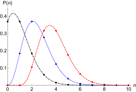
Figure 3: (color online) The photon number probability distributions for (a) an initial coherent state with a mean photon number of unity (black circles, dash-dotted line) (b) the state produced by a single photon addition (blue circles, dotted line) and (c) the state produced by two photon addition (red circles, dashed line). Photon subtraction leaves the initial coherent-state statistics unchanged.

We can extend this technique to find the photon number probability distribution after any number of photon additions, but present here only the example of two photon additions. After two successful photon addition processes our moment generating function is

$$\mathcal{N}^{2+}_{|\alpha\rangle}(\lambda) = \frac{e^{-|\alpha|^{2}}\exp\left(\frac{|\alpha|^{2}}{1+\lambda}\right)}{(1+\lambda)^{3}(|\alpha|^{4}+4|\alpha|^{2}+2)}$$ (57)

$$\qquad\times\left(2+\frac{4|\alpha|^{2}}{1+\lambda}+\frac{|\alpha|^{4}}{(1+\lambda)^{2}}\right).$$

From this we can readily extract the photon number probability distribution:

$$P^{2+}_{|\alpha\rangle}(n) = \frac{e^{-|\alpha|^{2}}}{(|\alpha|^{4}+4|\alpha|^{2}+2)}\left[2\frac{|\alpha|^{2(n-2)}}{(n-2)!}\right.$$ (58)

$$\>\>\left.+4|\alpha|^{2}\frac{|\alpha|^{2(n-3)}}{(n-3)!}+|\alpha|^{4}\frac{|\alpha|^{2(n-4))}}{(n-4)!}\right],$$

which comprises three shifted Poissonian distributions, shifted up by 2, 3 and 4 respectively.

In Fig. 3 we plot the photon number probability distributions for an initial coherent state with a mean photon number of unity and the distributions that result from successful one- and two-photon addition processes. The absence of a probability for the vacuum state in the former and for both the vacuum and one-photon states in the latter is readily apparent. It is also clear that adding a photon has the effect of broadening the probability distribution, what may be seen as a consequence of the combination of multiple shifted Poissonian distributions.

VI.2 Thermal states

The moment generating functions for the photon-subtracted and photon-added thermal states have the simple forms given in Eqs. (34) and (50). From the similarity in the forms of these it should come as no surprise that the statistics of an $\ell$-photon subtracted and an $\ell$-photon added thermal state are simply related. For this reason it is sensible to treat them together.

The simplest way to proceed is to expand the two moment generating functions $\mathcal{M}^{\ell-}_{\rm th}(\mu)$ and $\mathcal{N}^{\ell+}_{\rm th}(\lambda)$ as power series in $1-\mu$ and $1+\lambda$ respectively. This gives

$$\mathcal{M}^{\ell-}_{\rm th}(\mu) = (1+\mu\bar{n})^{-(\ell+1)}$$ (61)

$$= \left(\frac{1}{1+\bar{n}}\right)^{\ell+1}\sum_{m=0}^{\infty}\left(\frac{(1-\mu)\bar{n}}{1+\bar{n}}\right)^{m}\left(\begin{array}[]{c}\ell+m\\ \ell\end{array}\right),$$

which corresponds to a negative binomial probability distribution Jeffreys ; Lukacs ; Grimmett for the photon number

$$P^{\ell-}_{\rm th}(n)=\frac{\bar{n}^{n}}{(1+\bar{n})^{n+\ell+1}}\left(\begin{array}[]{c}\ell+n\\ \ell\end{array}\right).$$ (63)

For the photon-added thermal states we proceed in the same way but work with $\mathcal{N}(\lambda)$:

$$\mathcal{N}^{\ell+}_{\rm th}(\lambda) = [1+\lambda(1+\bar{n})]^{-(\ell+1)}$$ (66)

$$= \left(\frac{1}{(1+\lambda)(1+\bar{n})}\right)^{\ell+1}$$

$$\>\>\ \times\sum_{m=0}^{\infty}\left(\frac{\bar{n}}{(1+\lambda)(1+\bar{n})}\right)^{m}\left(\begin{array}[]{c}\ell+m\\ \ell\end{array}\right),$$

corresponding to another negative binomial distribution

$$P^{\ell+}_{\rm th}(n)=\frac{\bar{n}^{(n-\ell)}}{(1+\bar{n})^{n+1}}\left(\begin{array}[]{c}n\\ \ell\end{array}\right)\qquad(n\geq\ell).$$ (68)

For $n<\ell$ the probability is zero, which reflects the fact that $\ell$ photons have been added.

It is clear that the two photon probability distributions, Eqs. (63) and (68) are the same apart from a shift: they have the same shape but the probability distribution for the photon-subtracted states starts at zero photons, but that for the photon-added states starts, naturally, at $n=\ell$. This behaviour is clear in Figs. 4 and 5, which show the effects on the statistics of adding or subtracting one photon and of adding or subtracting two photons, respectively. The similarity in the distributions means that the statistics of photon-subtracted and photon-added thermal states are very similar. In particular, the mean photon number resulting from $\ell$-photon addition will exceed that resulting from $\ell$-photon subtraction by precisely $\ell$ and the variance in the photon number for the two states will be the same.

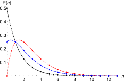
Figure 4: (color online) The photon number probability distributions for (a) an initial thermal state with a mean photon number of unity (black circles, dash-dotted line) (b) the state produced by a single photon subtraction (blue circles, dotted line) and (c) the state produced by single photon addition (red circles, dashed line).

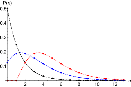
Figure 5: (color online) The photon number probability distributions for (a) an initial thermal state with a mean photon number of unity (black circles, dash-dotted line) (b) the state produced by a two photon subtraction (blue circles, dotted line) and (c) the state produced by a two photon addition (red circles, dashed line).

VI.3 Binomial and negative binomial states

Among the most important and most studied quantum optical processes are attenuation due to propagation through a lossy medium, and amplification using an inverted population or a parametric amplifier Methods ; Louisell1 ; Louisell2 ; MandelWolf . It should be emphasised that these processes are not simply related to the photon subtraction and addition processes discussed here. Rather they are processes formed by random combinations of successful and unsuccessful subtraction or addition events.

The effect of an ideal (zero-temperature) attenuator is to reduce the factorial moments by a factor depending on the strength of the attenuation:

$$\langle\hat{n}^{(m)}\rangle_{\rm Att.}=\eta^{m}\langle\hat{n}^{(m)}\rangle,$$ (69)

where $0\leq\eta<1$, with smaller values corresponding to stronger attenuation. It follows immediately, on using Eq. (94), that the moment generating function for the attenuated state has the same form as that for the pre-attenuated state, but with $\mu$ replaced by $\eta\mu$ Methods :

$$\mathcal{M}_{\rm Att.}(\mu)=\mathcal{M}(\eta\mu).$$ (70)

Moment generating functions have been used to describe the statistics of optical amplifiers LoudonShep ; ShepJakeman . Here we consider only the ideal case of a fully-inverted medium amplifier for which the mean photon number at the output is related to that at the input by

$$\langle\hat{n}\rangle_{\rm Amp.}=G\langle\hat{n}\rangle+G-1,$$ (71)

where $G\geq 1$ is the gain. More generally, we find that negative factorial moments are related simply to those for the input state

$$\langle(\hat{n}+1)^{(-m)}\rangle_{\rm Amp.}=G^{m}\langle(\hat{n}+1)^{(-m)}\rangle.$$ (72)

It follows, using Eq. (104), that the moment generating function (of the second kind) has the same form as that of the pre-amplified state, but with $\lambda$ replaced by $G\lambda$:

$$\mathcal{N}_{\rm Amp.}(\lambda)=\mathcal{N}(G\lambda).$$ (73)

The simple expressions, Eqs. (70) and (73), enable us to determine the effects of amplification or attenuation on the statistics of our photon-added states or, indeed, the effects of photon addition or subtraction on photo-subtracted or photon-added states. As an illustration, we consider photon subtraction or addition to an attenuated or amplified photon number state. The attenuated number state exhibits binomial statistics and the amplified number state has negative-binomial statistics. It is convenient to investigate these using the binomial Stoler and negative binomial states negbinomial .

VI.3.1 Binomial states

If we send an $M$-photon state through a lossy medium, in which the probability for any one photon to survive is $\eta$, then we end up with an incoherent mixture of number states in which the probability for $n$ photons to remain is

$$P^{\rm Att.}_{|M\rangle}(n)=\left(\begin{array}[]{c}M\\ n\end{array}\right)\eta^{n}(1-\eta)^{M-n}.$$ (74)

This mixed state has the same photon statistics as the pure binomial state $|\eta,M\rangle$ Stoler :

$$|\eta,M\rangle=\sum_{n=0}^{M}\left[\left(\begin{array}[]{c}M\\ n\end{array}\right)\eta^{n}(1-\eta)^{M-n}\right]^{1/2}|n\rangle.$$ (75)

There is no suggestion that this is the state produced by attenuation, but merely that it has the same photon statistics. The link with attenuation is simply one reason to consider the properties of the binomial states. Some of the principal properties of the binomial states are summarised in Appendix C.

The action of the annihilation operator on the binomial state $|\eta,M\rangle$ produces another binomial state, but with $M$ reduced by unity, see Eq. (110). It follows that the factorial moments for an $\ell$ photon subtracted binomial state are simply that for a binomial state with $M$ reduced by $\ell$:

$$\langle\hat{n}^{(m)}\rangle_{|\eta,M\rangle}^{\ell-} = \langle\hat{n}^{(m)}\rangle_{|\eta,M-\ell\rangle}$$ (76)

$$= \eta^{m}\frac{(M-\ell)!}{(M-m-\ell)!}.$$

This result has implications for a situation in which both photon addition and subtraction act to produce the final state. In particular, the form of the final state does not depend on the whether the subtraction occurs before, after or during the attenuation. The only difference is the success probability for the subtraction processes.

VI.3.2 Negative binomial states

Ideal amplification, with gain $G$, of an initial $M$-photon state produces an incoherent mixture of number states in which the probability for $n$ photons to be present is given by the negative binomial distribution,

$$P^{\rm Amp.}_{|M\rangle}(n)=\left(\begin{array}[]{c}n\\ M\end{array}\right)G^{-(M+1)}(1-G^{-1})^{n-M}.$$ (77)

This mixed state has the same photon statistics as the pure negative binomial state $|\eta,-(M+1)\rangle$ negbinomial with gain $G=\eta^{-1}$ negbinomial :

$$|\eta,-(M+1)\rangle=\sum_{n=M}^{\infty}\left[\left(\begin{array}[]{c}n\\ M\end{array}\right)\eta^{M+1}(1-\eta)^{n-M}\right]^{1/2}|n\rangle.$$ (78)

As with attenuation and the binomial states, there is no suggestion that this is the state produced by amplification, but merely that it has the same photon statistics. The link with amplification is simply one reason to consider the properties of the negative binomial states, some of the properties of which are presented in Appendix C.

The action of the creation operator on the negative binomial state $|\eta,-(M+1)\rangle$ produces another negative binomial state, but with $M$ increased by unity, as in Eq. (118). Hence the negative factorial moments for an $\ell$-photon added negative binomial state are those for a negative binomial state with $M$ increased by $\ell$:

$$\langle(\hat{n}+1)^{(-m)}\rangle_{|\eta,-(M+1)\rangle}^{\ell-} = \langle(\hat{n}+1)^{(-m)}\rangle_{|\eta,-(M+\ell+1)\rangle}$$ (79)

$$= \eta^{-m}\frac{(M+\ell+m)!}{(M+\ell)!}.$$

We note that, as with the corresponding result for the binomial states, this expression tells us that the form of the state produced by a combination of amplification and photon addition does not depend on the order in which these processes are applied.

VI.3.3 Agarwal’s negative binomial states

As noted above, Agarwal defined negative binomial states somewhat differently, with a photon number probability distribution starting at $n=0$ rather than at $n=M$ so that the photon number probability distribution is AgarwalNeg

$$P_{\rm Agar}(n)=\left(\begin{array}[]{c}n+s\\ n\end{array}\right)\beta^{s+1}(1-\beta)^{n}.$$ (80)

To see the connection with the states $|\eta,-(M+1)\rangle$ let us rewrite these probabilities in a different notation:

$$P_{\rm Agar}(n)=\left(\begin{array}[]{c}n+M\\ M\end{array}\right)\eta^{M+1}(1-\eta)^{n}.$$ (81)

It is clear from this that

$$P_{\rm Agar}(n)=P_{|\eta,-(M+1)\rangle}(n+M).$$ (82)

The moment generating function of the second kind for this state is

$$\mathcal{N}_{\rm Agar}(\lambda)=\frac{1}{1+\lambda}\left[\frac{\eta(1+\lambda)}{\lambda+\eta}\right]^{M+1}$$ (83)

from which it is straightforward to calculate the negative factorial moments. For the first of these we find

$$\langle\hat{n}+1\rangle = \left.-\frac{d}{d\lambda}\mathcal{N}_{\rm Agar}(\lambda)\right|_{\lambda=0}$$ (84)

$$= \frac{M+1}{\eta}-M.$$

We note that this is $M$ less than the corresponding value for the state $|\eta,-(M+1)\rangle$, as it should be.

VII Conclusions

Experiments realising both photon subtraction and photon addition have been shown to lead to novel quantum states Philippe and have been employed to test one of the most fundamental ideas in quantum optics Bellini1 ; Bellini2 ; Bellini3 . It has been shown, moreover, that these processes can lead to, at first sight, surprising phenomena in optical measurements Bobexpt ; Lanz . These developments motivated the study presented here. We have shown how the statistics of the states produced by photon subtraction and photon addition can be derived directly and simply from those of the original state. The natural tools for this are the moment generating function $\mathcal{M}(\mu)$, familiar to quantum optics Methods , and a second, closely related function $\mathcal{N}(\lambda)$, which we introduce here.

We have presented a comprehensive study of the statistics of photon subtracted and photon added states. We have found, in particular, that photon subtraction will result in a increase in the mean photon number if the initial state was super-Poissonian and that successful photon addition will, except for an initial number state, increase the mean photon number by more than the number of photons added and that photon subtraction leaves the mean photon number, and indeed the full probability distribution, unchanged. We have seen that the resolution of these apparently paradoxical behaviours lies in the fact that the processes are necessarily probabilistic and that the photon number probability distribution for the incident light given that the subsequent process of subtraction or addition is successful is not the same as the initial distribution. The explanation for these behaviours lies, as is so often the case, in the correct application of Bayes’ theorem.

Appendix A Moment generating functions

A.1 $\mathcal{M}(\mu)$

Our first moment generating function is

$$\mathcal{M}(\mu)=\sum_{n=0}^{\infty}(1-\mu)^{n}P(n).$$ (85)

This function was once a commonly employed tool in quantum optics. Its values and those of its derivatives provide a wealth of information. In particular the derivatives evaluated at $\mu=1$ give the photon-number probabilities:

$$P(n)=\frac{1}{n!}\left.\left(-\frac{d}{d\mu}\right)^{n}\mathcal{M}\right|_{\mu=1}.$$ (86)

The derivatives evaluated at $\mu=0$ give the factorial moments:

$$\langle\hat{n}^{(m)}\rangle = \langle\hat{n}(\hat{n}-1)\cdots(\hat{n}-m+1)\rangle$$ (87)

$$= \left.\left(-\frac{d}{d\mu}\right)^{m}\mathcal{M}(\mu)\right|_{\mu=0}.$$

The first few of these are

$$\mathcal{M}(0) = 1$$

$$-\frac{d}{d\mu}\mathcal{M}(0) = \langle\hat{n}\rangle$$

$$\frac{d^{2}}{d\mu^{2}}\mathcal{M}(0) = \langle\hat{n}(\hat{n}-1)\rangle=\langle\mathop{:}\nolimits\!\hat{n}^{2}\!\mathop{:}\nolimits\rangle,$$ (88)

where the dots $\mathop{:}\nolimits\!~{}\!\mathop{:}\nolimits$ denote normal ordering. More generally the factorial moment $\langle\hat{n}^{(m)}\rangle$ is the normal ordered expectation value of the $\hat{n}^{m}$, so that $\langle\hat{n}^{(m)}\rangle=\langle\mathop{:}\nolimits\!\hat{n}^{m}\!\mathop{:}\nolimits\rangle=\langle\hat{a}^{\dagger m}\hat{a}^{m}\rangle$.

We can also extract the moments of the photon number by differentiation. To this end we introduce the change of variable, $x=\ln(1-\mu)$, so that

$$\mathcal{M}=\sum_{n=0}^{\infty}e^{nx}P(n).$$ (89)

It follows that the required moments are simply derivatives with respect to $x$ evaluated at $x=0$ (or $\mu=1$):

$$\langle\hat{n}^{m}\rangle=\left.\left(\frac{d}{dx}\right)^{m}\mathcal{M}\right|_{x=0}.$$ (90)

One additional property that we make use of is the fact that $\mathcal{M}(2)$ reveals the probabilities that the number of photons is either even or odd:

$$\mathcal{M}(2)=P({\rm even})-P({\rm odd}).$$ (91)

Part of the utility of the moment generating function arises from the fact that its evolution can be readily calculated in a number of situations including both linear amplification and loss. It is also possible to evaluate it directly from the quasi-probability phase-space distributions. In particular, it has a simple form in terms of the Glauber-Sudarshan P function:

$$\mathcal{M}(\mu)=\int d^{2}\alpha e^{-\mu|\alpha|^{2}}P(\alpha).$$ (92)

This follows directly from the operator ordering theorem

$$(1-\mu)^{\hat{n}}=\mathop{:}\nolimits\!e^{-\mu\hat{n}}\!\mathop{:}\nolimits\,.$$ (93)

If we take the expectation value of this operator we find an expression for the moment generating function in terms of the factorial moments:

$$\mathcal{M}(\mu)=\sum_{m=0}^{\infty}\frac{(-\mu)^{m}}{m!}\langle\hat{n}^{(m)}\rangle,$$ (94)

the Maclaurin series of which gives the factorial moments as in Eq. (87). It should be emphasised, however, that the integral form Eq. (92) may run into convergence problems for some states and for certain values of $\mu$. When such difficulties arise, the original form Eq. (85) should be used.

A.2 $\mathcal{N}(\lambda)$

Our second moment generating function is

$$\mathcal{N}(\lambda)=\sum_{n=0}^{\infty}(1+\lambda)^{-(n+1)}P(n).$$ (95)

The first thing that should be noted is that this function is simply related to the first moment generating function,

$$\mathcal{N}(\lambda) = \frac{1}{1+\lambda}\mathcal{M}\left(\frac{\lambda}{1+\lambda}\right)$$

$$\mathcal{M}(\mu) = \frac{1}{1-\mu}\mathcal{N}\left(\frac{\mu}{1-\mu}\right),$$ (96)

but it proves convenient to introduce it as a separate function because of its distinctive properties. Principal among these is the ease with which we can generate negative or ascending factorial moments:

$$\langle(\hat{n}+1)^{(-m)}\rangle=\langle(\hat{n}+1)(\hat{n}+2)\cdots(\hat{n}+m)\rangle,$$ (97)

where $x^{(-m)}$ denotes the ascending factorial Steffensen or Pochhammer symbol Abram ; Olver

$$x^{(-m)}=x(x+1)\cdots(x+m-1)$$ (98)

The negative factorial moments are simply the expectation values of the corresponding powers of the number operator in antinormal order:

$$\langle(\hat{n}+1)^{(-m)}\rangle=\langle\mathop{\scriptscriptstyle{\bm{\vdots}}}\nolimits\!\hat{n}^{m}\!\mathop{\scriptscriptstyle{\bm{\vdots}}}\nolimits\rangle,$$ (99)

where the dots $\mathop{\scriptscriptstyle{\boldsymbol{\bm{\vdots}}}}\nolimits\!~{}\!\mathop{\scriptscriptstyle{\boldsymbol{\bm{\vdots}}}}\nolimits$ denote antinormal order, that is $\langle\mathop{\scriptscriptstyle{\bm{\vdots}}}\nolimits\!\hat{n}^{m}\!\mathop{\scriptscriptstyle{\bm{\vdots}}}\nolimits\rangle=\langle\hat{a}^{m}\hat{a}^{\dagger m}\rangle$. The negative factorial moments are obtained from $\mathcal{N}(\mu)$ by differentiation in an analogous manner to the factorial moments from $\mathcal{M}(\mu)$:

$$\langle(\hat{n}+1)^{(-m)}\rangle=\left.\left(-\frac{d}{d\lambda}\right)^{m}\mathcal{N}(\lambda)\right|_{\lambda=0}.$$ (100)

We note also that the function $\mathcal{N}(\lambda)$ provides other information including the probability that the photon number is even or odd:

$$\mathcal{N}(-2)=P({\rm odd})-P({\rm even})=-\mathcal{M}(2).$$ (101)

It is also simply related to the Husimi or Q quasi-probability distribution:

$$\mathcal{N}(\lambda)=\int d^{2}\alpha e^{-\lambda|\alpha|^{2}}Q(\alpha),$$ (102)

which follows from the operator identity

$$(1+\lambda)^{-(\hat{n}+1)}=\mathop{\scriptscriptstyle{\bm{\vdots}}}\nolimits\!e^{-\lambda\hat{n}}\!\mathop{\scriptscriptstyle{\bm{\vdots}}}\nolimits\,.$$ (103)

If we take the expectation value of this operator we find an expression for the moment generating function in terms of the negative factorial moments:

$$\mathcal{N}(\lambda)=\sum_{m=0}^{\infty}\frac{(-\lambda)^{m}}{m!}\langle(\hat{n}+1)^{(-m)}\rangle,$$ (104)

the Maclaurin series of which gives the negative factorial moments as in Eq. (100). As with our first moment generating function, the integral form given here, in Eq. (102), may have convergence problems for some values of $\lambda$. In such cases the original form, Eq. (95) should be used.

Finally, we note that the photon number probability distribution can be obtained from $\mathcal{N}(\lambda)$ by differentiation:

$$P(n)=\lim_{\lambda\rightarrow\infty}\frac{(1+\lambda)^{n+1}}{n!}\left(-\frac{d}{d\lambda}\right)^{n}(1+\lambda)^{n}\mathcal{N}(\lambda).$$ (105)

Appendix B Derivation of an inequality

We require the inequality

$$\langle(\hat{n}+1)(\hat{n}+1)\cdots(\hat{n}+\ell)\rangle\geq\langle(\hat{n}+1)\cdots(\hat{n}+\ell)\rangle\langle(\hat{n}+1)\rangle$$ (106)

in the derivation of Eq. (46). To establish this let us consider, first, a more general combination:

$$\langle B(\hat{n})A(\hat{n})\rangle - \langle B(\hat{n})\rangle\langle A(\hat{n})\rangle$$

$$\qquad= \sum_{n}P(n)B(n)A(n)$$

$$\quad-\sum_{n}\sum_{m}P(n)P(m)B(n)A(m)$$

$$\qquad= \sum_{n}\sum_{m}P(n)P(m)B(n)A(n)$$

$$\quad-\sum_{n}\sum_{m}P(n)P(m)B(n)A(m)$$

$$\qquad= \frac{1}{2}\sum_{m}\sum_{n}P(n)P(m)[A(m)-A(n)]$$ (107)

$$\qquad\times[B(m)-B(n)].$$

For $A(n)=n+1$ and $B(n)=(n+1)\cdots(n+\ell)$ the combinations $A(m)-A(n)$ and $B(m)-B(n)$ are either both positive or both negative for all $m\neq n$ and hence the terms in the summation are all greater than or equal to zero and the inequality Eq. (106) follows. Note that for this reason the equality in Eq. (106) holds if and only if $P(n)=\delta_{n,N}$ for some $N$ corresponding to photon number state.

Appendix C Binomial and negative binomial states

The binomial and negative binomial states are pure states for which the photon number probabilities correspond to the binomial and negative binomial distributions respectively. We summarise here some of the more important properties of these states.

C.1 Binomial states

The binomial states are defined to be pure states with a photon number probability distribution that is of binomial form Stoler :

$$|\eta,M\rangle=\sum_{n=0}^{M}\beta_{n}^{M}|n\rangle,$$ (108)

where

$$\beta_{n}^{M}=\left[\left(\begin{array}[]{c}M\\ n\end{array}\right)\eta^{n}(1-\eta)^{M-n}\right]^{1/2}.$$ (109)

Here $M$ is a non-negative integer and $\eta$ can take any value between $0$ and $1$. The action of the annihilation operator on this state produces another binomial state, one with $M$ reduced by unity:

$$\hat{a}|\eta,M\rangle=\sqrt{\eta M}|\eta,M-1\rangle.$$ (110)

It follows that the mean photon number for this state is $\eta M$ and, more generally, the factorial moments for this state are

$$\langle\hat{n}^{(m)}\rangle=\eta^{m}\frac{M!}{(M-m)!}.$$ (111)

This means, in particular, that the states exhibit sub-Poissionian statistics, with a normally-ordered photon number variance that is negative:

$$:\Delta n^{2}:=\langle\hat{n}^{(2)}\rangle-\langle\hat{n}\rangle^{2}=-\eta^{2}M.$$ (112)

If we generalise the states to include a phase,

$$|\eta,M,\theta\rangle=\sum_{n=0}^{M}\beta_{n}^{M}e^{in\theta}|n\rangle,$$ (113)

then we have an over-complete set of states. To see this we need only note that the states are, in general, not orthogonal but can be used to represent the identity operator:

$$\frac{1}{2\pi}\int_{0}^{2\pi}d\theta \eta \sum_{M=0}^{\infty}|\eta,M,\theta\rangle\langle\eta,M,\theta|$$ (114)

$$\qquad=\sum_{M=0}^{\infty}\sum_{n=0}^{M}\eta\left(\beta_{n}^{M}\right)^{2}|n\rangle\langle n|$$

$$\qquad=\sum_{n=0}^{\infty}|n\rangle\langle n|$$

$$\qquad=\hat{\rm I}.$$

For example, the mixed state produced by attenuating the photon number state $|M\rangle$ has the density operator

$$\hat{\rho}^{\rm Att.}_{|M\rangle}=\frac{1}{2\pi}\int_{0}^{2\pi}d\theta|\eta,M,\theta\rangle\langle\eta,M,\theta|.$$ (115)

Further properties of this state may be found in Stoler .

C.2 Negative binomial states

The negative binomial states are defined to be pure states with a photon number probability distribution that is of negative binomial form negbinomial :

$$|\eta,-(M+1)\rangle=\sum_{n=M}^{\infty}\beta_{n}^{-(M+1)}|n\rangle,$$ (116)

where

$$\beta_{n}^{-(M+1)}=\left[\left(\begin{array}[]{c}n\\ M\end{array}\right)\eta^{M+1}(1-\eta)^{n-M}\right]^{1/2}.$$ (117)

Here $M$ is again a non-negative integer and $\eta$ can take any value between $0$ and $1$. For these states it is the action of the creation operator that is simple:

$$\hat{a}^{\dagger}|\eta,-(M+1)\rangle=\sqrt{\frac{M+1}{\eta}}|\eta,-(M+2)\rangle.$$ (118)

It follows that the mean photon number for this state is $(M+1)/\eta-1$ and, more generally, that the negative factorial moments for this state have the form

$$\langle(\hat{n}+1)^{(-m)}\rangle=\eta^{-m}\frac{(M+m)!}{M!},$$ (119)

so that the antinormally ordered variance in the photon number is

$$\dot{:}\Delta n^{2}\dot{:}=\langle(\hat{n}+1)^{(-2)}\rangle-\langle(\hat{n}+1)\rangle^{2}=\frac{M+1}{\eta^{2}}.$$ (120)

As with the binomial states, we can generalise the negative binomial states by including a phase

$$|\eta,-(M+1),\theta\rangle=\sum_{n=0}^{M}\beta_{n}^{-(M+1)}e^{in\theta}|n\rangle,$$ (121)

with the resulting set of states being overcomplete so that they form a resolution of the identity:

$$\frac{1}{2\pi}\int_{0}^{2\pi}d\theta \eta^{-1} \sum_{M=0}^{\infty}|\eta,-(M+1),\theta\rangle\langle\eta,-(M+1),\theta|$$ (122)

$$\qquad=\sum_{M=0}^{\infty}\sum_{n=M}^{\infty}\eta^{-1}\left(\beta_{n}^{-(M+1)}\right)^{2}|n\rangle\langle n|$$

$$\qquad=\sum_{n=0}^{\infty}|n\rangle\langle n|$$

$$\qquad=\hat{\rm I}.$$

In particular, the mixed state produced by amplifying the photon number state $|M\rangle$ with a gain $G=\eta^{-1}$ has the density operator

$$\hat{\rho}^{\rm Amp.}_{|M\rangle}=\frac{1}{2\pi}\int_{0}^{2\pi}d\theta|\eta,-(M+1),\theta\rangle\langle\eta,-(M+1),\theta|.$$ (123)

Further properties of this state may be found in negbinomial .

References

- (1) J. Wenger, R. Tualle-Brouri and P. Grangier, Non-Gaussian statistics from individual pulses of squeezed light, Phys. Rev. Lett. 92, 153601 (2004).
- (2) V. Parigi, A. Zavatta, M. S. Kim and M. Bellini, Probing quantum commutation rules by addition and subtraction of single photons to/from a light field, Science 317, 1890 (2007).
- (3) M. S. Kim, H. Jeong, A. Zavatta, V. Parigi and M. Bellini, Scheme for probing the bosonic commutation relation using single-photon interference, Phys. Rev. Lett. 101, 260401 (2008).
- (4) A. Zavatta, V. Parigi, M. S. Kim, H. Jeong and M. Bellini, Experimental demonstration of the bosonic commutation relation via superpositions of quantum operations on thermal light fields, Phys. Rev. Lett. 103, 140406 (2009).
- (5) G. S. Agarwal, Quantum Optics (Cambridge University Press, Cambridge, 2013).
- (6) S. Loepp and W. K. Wootters, Protecting Information (Cambridge University Press, Cambridge, 2006).
- (7) G. Van Assche. Quantum Cryptography and Secret-Key Distillation (Cambridge University Press, Cambridge, 2006).
- (8) S. M. Barnett Quantum Information (Oxford University Press, Oxford, 2009).
- (9) S. M. H. Rafsanjani, M. Mirhosseini, O. S. Magaña-Loaiza, B. T. Gard, R. Birrittella, B. E. Koltenbah, C. G. Parazzoli, B. A. Capron, C. C. Gerry, J. P. Dowling and R. W. Boyd, Quantum-enhanced interferometry with weak thermal light, Optica 4, 487 (2017).
- (10) E. Lanz, Quantum-enhanced interferometry with weak thermal light: comment, Optica 4, 1314 (2017).
- (11) D. Braun, P. Jian, O. Pinel and N. Treps, Precision measurements with photon-subtracted or photon-added Gaussian states, Phys. Rev. A 90, 013821 (2014).
- (12) A. Mari and J. Eisert, Positive Wigner functions render classical simulation of quantum computation efficient, Phys. Rev. Lett. 109, 230503 (2012).
- (13) M. Gu, C. Weedbrook, N. C. Menicucci, T. C. Ralph and P. van Loock, Quantum computing with continuous-variable clusters, Phys. Rev. A 79, 062318 (2009).
- (14) T. Douce, D. Markham, E. Kashefi, E. Diamanti, T. Coudreau, P. Milman, P. van Loock and G. Ferrini, Continuous-variable instantaneous quantum computing is hard to sample, Phys. Rev. Lett. 118, 070503 (2017).
- (15) M. Walschaers, C. Fabre, V. Parigi and N. Treps, Entanglement of multimode non-Gaussian states, Phys. Rev. Lett. 119, 183601 (2017).
- (16) M. D. Vidrighin, O. Dahlsten, M. Barbieri, M. S. Kim, V. Vedral and I. A. Walmsley, Photonic Maxwell’s demon, Phys. Rev. Lett. 116, 050401 (2016).
- (17) G. S. Agarwal and K. Tara, Nonclassical properties of states generated by the excitations of a coherent state, Phys. Rev. A 43, 492 (1991).
- (18) G. S. Agarwal, Negative binomial states of the field-operator representation and production by state reduction in optical processes, Phys. Rev. A 45, 1787 (1992).
- (19) M. S. Kim, E. Park, P. L. Knight and H. Jeong, Nonclassicality of a photon-subtracted Gaussian field, Phys. Rev. A 71, 043805 (2005).
- (20) A. Ourjoumtsev, R. Tualle-Brouri, J. Laurat and P. Grangier, Generating optical Schödinger kittens for quantum information processing, Science 312, 83 (2006).
- (21) J. S. Neergaard-Nielsen, B. M. Nielsen, C. Hettich, K. Mølmer and E. S. Polzik, Generation of a superposition of odd photon number states for quantum information networks, Phys. Rev. Lett. 97, 083604 (2006).
- (22) A. Biswas and G. S. Agarwal, Nonclassicality and decoherence of photon-subtracted squeezed states, Phys. Rev. A 75, 032104 (2007).
- (23) J. Fiurášek, Engineering quantum operations on travelling light beams by multiple photon addition and subtraction, Phys. Rev. A 80, 053822 (2009).
- (24) Yu. I. Bogdanov, K. G. Katamadze, G. V. Avosopiants, I. V. Belinsky, N. A. Bogdanova, A. A. Kalinkin and S. P. Kulik, Multiphoton subtracted thermal states: description, preparation, and reconstruction, Phys. Rev. A 96, 063803 (2017).
- (25) H. Carmichael, An Open Systems Approach to Quantum Optics (Springer-Verlag, Berlin, 1991).
- (26) K. Mølmer, Y. Castin and J. Dalibard, Monte-Carlo wave-function method in quantum optics, J. Opt. Soc. Am. B 10, 524 (1993).
- (27) C. W. Gardiner and P. Zoller, Quantum Noise 3rd ed. (Springer, Berlin, 2004).
- (28) H. J. Carmichael, Statistical Methods in Quantum Optics 2 (Springer, Berlin, 2008).
- (29) B. M. Garraway and P. L. Knight, Evolution of quantum superpositions in open environments: quantum trajectories, jumps, and localization in phase space, Phys. Rev. A 50, 2548 (1994).
- (30) S. M. Barnett and P. L. Knight, Dissipation in a fundamental model of quantum optical resonance, Phys. Rev. A 33, 2444 (1986).
- (31) S. M. Barnett and J. Jeffers, The damped Jaynes-Cummings model, J. Mod. Opt. 54, 2033 (2007).
- (32) J. Calsamiglia, S. M. Barnett, N. Lütkenhaus and K.-A. Suominen, Removal of a single photon by adaptive absorption, Phys. Rev. A 64, 043814 (2001).
- (33) D. K. L. Oi, V. Potoček and J. Jeffers, Nondemolition measurement of the vacuum state or its complement, Phys. Rev. Lett. 110, 210504 (2013).
- (34) S. Rosenblum, O. Bechler, I. Shomroni, Y. Lovski, G. Guendelman and B. Dayan, Extraction of a single photon from an optical pulse, Nat. Photon. 10, 19 (2016).
- (35) S. M. Barnett and P. M. Radmore, Methods in Theoretical Quantum Optics (Oxford University Press, Oxford, 1997).
- (36) M. Ueda, N. Imoto and T. Ogawa, Quantum theory for continuous photodetection processes, Phys. Rev. A 41, 3891 (1990).
- (37) M. Ban, Quasicontinuous measurements of photon number, Phys. Rev. A 49, 5078 (1994).
- (38) A. Zavatta, V. Parigi, M. S. Kim and M. Bellini, Subtracting photons from arbitrary light fields: experimental test of coherent invariance by single-photon annihilation, New J. Phys. 10, 123006 (2008).
- (39) S. S. Mizrahi and V. V. Dodonov, Creating quanta with an ‘annihilation’ operator, J. Phys. A: Math. Gen. 35, 8847 (2002).
- (40) H. Jeffreys, Theory of Probability (Oxford University Press, Oxford, 1939).
- (41) E. Lukacs, Characteristic Functions (Griffin and Co., London, 1960).
- (42) C. W. Helstrom, Statistical theory of signal detection 2nd ed. (Pergamon Press, Oxford, 1968).
- (43) A. Rényi, Foundations of Probability (Holden-Day, San Francisco CA, 1970).
- (44) N. G. van Kampen, Stochastic Processes in Physics and Chemistry 3rd ed. (Elsevier, Amsterdam, 2007).
- (45) C. W. Gardiner, Handbook of Stochastic Methods (Springer-Verlag, Berlin, 1985).
- (46) G. Grimmett and D. Welsh, Probability: An Introduction 2nd ed. (Oxford University Press, Oxford, 2014).
- (47) R. J. Glauber, Optical coherence and photon statistics, in D. de Witt, A. Blandin and C. Cohen-Tannoudji eds. Quantum Optics and Electronics (Gordon and Breach, New York, 1965). Reprinted in R. J. Glauber Quantum Theory of Coherence (Wiley-VCH, Weinheim, 2007).
- (48) E. Jakeman and E. R. Pike, The intensity-fluctuation distribution of Gaussian light, J. Phys. A (Proc. Phys. Soc.)1 128, (1968).
- (49) R. Loudon, The Quantum Theory of Light 3rd ed. (Oxford University Press, Oxford, 2000).
- (50) G. E. P. Box and G. C. Tiao, Bayesian Inference in Statistical Analysis (Wiley, New York, 1973).
- (51) D. J. Mackay, Information Theory, Inference, and Learning Algorithms (Cambridge University Press, Cambridge, 2003).
- (52) J. F. Steffensen, Interpolation 2nd ed. (Chelsea Publishing, New York, 1950).
- (53) P. A. M. Dirac, The Principles of Quantum Mechanics 4th ed. (Oxford University Press, Oxford, 1958).
- (54) D. Stoler, B. E. A. Saleh and M. C. Teich, Binomial states of the quantized radiation field, Optica Acta 32, 345 (1985).
- (55) S. M. Barnett, Negative binomial states of the quantized radiation field, J. Mod. Opt. 45, 2201 (1998). It should be noted that these states are distinct form those introduced by Agarwal AgarwalNeg .
- (56) W. H. Louisell, Radiation and Noise in Quantum Electronics (McGraw-Hill, New York, 1964).
- (57) W. H. Louisell, Quantum Statistical Properties of Radiation (Wiley, New York, 1973).
- (58) L. Mandel and E. Wolf, Optical Coherence and Quantum Optics (Cambridge University Press, Cambridge, 1995).
- (59) R. Loudon and T. J. Shepherd, Properties of the optical quantum amplifier, Optica Acta 31, 1243 (1984).
- (60) T. J. Shepherd and E. Jakeman, Statistical analysis of an incoherently coupled, steady-state optical amplifer, J. Opt. Soc. Am. B 4, 1860 (1987).
- (61) M. Abramowitz and I. A. Stegun eds. Handbook of Mathematical Functions (Dover, New York, 1965).
- (62) F. W. J. Olver, Introduction to Asymptotics and Special Functions (Academic Press, New York, 1974).