Approximate Bayesian inference for mixture cure models

Abstract

Cure models in survival analysis deal with populations in which a part of the individuals cannot experience the event of interest. Mixture cure models consider the target population as a mixture of susceptible and non-susceptible individuals. The statistical analysis of these models focuses on examining the probability of cure (incidence model) and inferring on the time-to-event in the susceptible subpopulation (latency model).

Bayesian inference on mixture cure models has typically relied upon Markov chain Monte Carlo (MCMC) methods. The integrated nested Laplace approximation (INLA) is a recent and attractive approach for doing Bayesian inference. INLA in its natural definition cannot fit mixture models but recent research has new proposals that combine INLA and MCMC methods to extend its applicability to them (Bivand et al., 2014; Gómez-Rubio and Rue, 2017; Gómez-Rubio, 2018).

This paper focuses on the implementation of INLA in mixture cure models. A general mixture cure survival model with covariate information for the latency and the incidence model within a general scenario with censored and non-censored information is discussed. The fact that non-censored individuals undoubtedly belong to the uncured population is a valuable information that was incorporated in the inferential process.

1 Introduction

Survival analysis is an area of statistics dedicated to researching time-to-event data. This is one of the oldest areas of statistics, which dates back to the 1600s with the construction of life tables. The study of time-to-event data seems simple and traditional because its main focus is centered on non-negative random variables. But this is very far from being the case. The fact that survival times are always positive keeps it away from the normal distribution framework, censoring and truncation schemes produce non-traditional likelihood issues, and the special elements that generate the dynamic nature of events occurring in time make survival analysis an interesting and exciting area of research and application, mainly in the biomedical field.

Cure models in survival analysis deal with target populations in which a part of the individuals cannot experience the event of interest. This type of models have largely been developed as a consequence of the discovery and development of new treatments against cancer. The rationale of considering a cure subpopulation comes from the idea that a successful treatment removes totally the original tumor and the individual cannot experience any recurrence of the disease. These models allow to estimate the probability of cure, a key and valuable outcome in cancer research. This is not the case for the traditional survival models which consider that all the individuals in the population are at risk. As stated by Lambert et al. (2007), it is important to bear in mind that cure is considered from a statistical, population point of view and not from an individual perspective.

Mixture cure models are the most popular cure models. They consider that the target population is a mixture of susceptible and non-susceptible individuals. The main interest focuses on the so called incidence model, that accounts for the probability of cure, and the latency model for the time-to-event in the susceptible subpopulation. A mixture model such as this is very attractive, easy to interpret, and allows to account for model complexity (frailties, time-dependent covariates, etc) in both incidence and latency terms (Peng and Taylor, 2014). Some studies in cancer research with this type of models are Sposto (2002) who discussed data from trials in paediatric cancer conducted by the Children’s Cancer Group, (Rondeau et al., 2013) who studied recurrences for breast cancer and readmissions for colorectal cancer, and (Hurtado Rúa and Dey, 2016) who centered on melanoma cancer. A very interesting review of these models up to date is (Peng and Taylor, 2014). Cured models also appear in other areas of research. This is the case of split population models in economics (Schmidt and Witte, 1989) and limited-failure population life models in reliability (Meeker, 1987).

Bayesian inference always expresses uncertainty in terms of probability distributions (Loredo, 1989, 1992) and uses Bayes’ theorem as often as necessary in a sequential way to update all relevant information. Bayesian methodology is especially attractive for survival analysis due to its natural treatment of censoring and truncation schemes as well as the probabilistic quantification of relevant survival outcomes, such as survival probabilities, that they do not need to resort to asymptotic tools (Ibrahim et al., 2001).

Computation in Bayesian inference is a key issue that allows the approximate implementation of non-analytical posterior distributions. The integrated nested Laplace approximation (INLA) (Rue et al., 2009) is a recent methodology for doing approximate Bayesian inference in the framework of latent Gaussian models (LGM) (Rue and Held, 2005). These models are a special class of Bayesian additive models that cover a wide range of studies and applications (Rue et al., 2017), and survival models in particular (Martino et al., 2011). INLA, in comparison to Markov chain Monte Carlo (MCMC) methods, provides accurate and fast approximations to the relevant posterior marginal distributions.

INLA is very attractive and has very good properties but it also has some limitations. In particular, INLA cannot fit mixture models (Marin et al., 2005) in a natural way because they are generally defined in terms of a combination of different distributions (Gómez-Rubio and Rue, 2017). But in science, every constraint or difficulty becomes an opportunity for learning. On this matter, (Bivand et al., 2014) and (Gómez-Rubio and Rue, 2017) propose the combination of INLA within MCMC for mixture models, in particular Gibbs sampling, and fit with INLA the relevant posterior conditional distributions. (Gómez-Rubio, 2018) extends these proposals and introduce Modal Gibbs sampling to accelerate the inferential process.

This paper focuses on the implementation of INLA in mixture cure models. A general mixture cure survival model with covariate information for the latency and the incidence model within a general scenario with censored and non-censored information is discussed. The fact that non-censored individuals undoubtedly belong to the uncured population is a valuable information that was incorporated in the inferential process.

The organization of this paper is as follows. Section 2 presents the main elements of mixture cure models and the two most popular mixture cure models, the Cox proportional hazards and the accelerated failure times models. Section 3 introduces the integrated nested Laplace approximation within the general framework of Bayesian inference. Section 4 is the core of the paper and contains our INLA proposal for estimating mixture cure models. Section 5 applies our proposal to the statistical analysis of two benchmark data sets in the framework of clinical trials and bone marrow transplants, and discusses and compares the subsequent results with those from a MCMC implementation. The paper ends with some conclusions.

2 Mixture cure models

Let $T^{*}$ be a continuous and non-negative random variable that describes the time-to-event of an individual in some target population. Let $Z$ be a cure random variable defined as $Z=0$ if that individual is susceptible for experiencing the event of interest, and $Z=1$ if she/he is cured or immune for that event. Cure and non cure probabilities are $P(Z=1)=\eta$ and $P(Z=0)=1-\eta$, respectively. The survival function for individuals in the cured and uncured population, $S_{c}(t)$ and $S_{u}(t)$, $t>0$, respectively, is

$$S_{u}(t)= \,\,P(T^{*}>t\mid Z=0)$$

$$S_{c}(t)= \,\,P(T^{*}>t\mid Z=1)=1.$$ (1)

The general survival function for $T^{*}$ can be expressed in terms of a mixture of both cured and uncured populations in the form

$$S(t)=\,\,P(T^{*}>t)=\eta+(1-\eta)\,S_{u}(t).$$ (2)

It is important to point out that $S_{u}(t)$ is a proper survival function but $S(t)$ is not. It goes to $\eta$ and not to zero when $t$ goes to infinity. Cure fraction $\eta$ is also known as the incidence model and time-to-event $T^{*}_{u}$ in the uncured population as the latency model (Peng and Taylor, 2014).

2.1 Covariates in the incidence model

The effect of a baseline covariate vector $\boldsymbol{x}_{1}$ on the cure proportion is typically modeled by means of a logistic link function, $\mbox{logit}[\eta(\boldsymbol{\beta}_{1})]=\boldsymbol{\beta}_{1}^{\prime}\boldsymbol{x}_{1}$, also expressed as

$$\eta(\boldsymbol{\beta}_{1})=\dfrac{\mbox{exp}\{\boldsymbol{\beta}_{1}^{\prime}\boldsymbol{x}_{1}\}}{1+\mbox{exp}\{\boldsymbol{\beta}_{1}^{\prime}\boldsymbol{x}_{1}\}},$$ (3)

where $\boldsymbol{\beta}_{1}$ is the vector of regression coefficients associated to $\boldsymbol{x}_{1}$. Note that other link functions can be used to connect the cure fraction with the vector of covariates $\boldsymbol{x}_{1}$ such as the probit link or the complementary log-log link (see Robinson (2014) for more details).

2.2 Covariates in the latency model

The most common regression models in survival analysis are the Cox proportional hazards model (Cox, 1972) and the accelerated failure time models. We will introduce them below.
Cox proportional hazards model, CPH. It is usually formulated in terms of the hazard function for the time-to-event $T_{u}^{*}$, or instantaneous rate of occurrence of the event, as

$$h_{u}(t\mid h_{u0},\boldsymbol{\beta}_{2}) =\,\lim_{\Delta t\to\infty}\frac{P(t\leq T_{u}^{*}<t+\Delta t\mid T\geq t)}{\Delta t}$$

$$=\,h_{u0}(t)\,\mbox{exp}\{\boldsymbol{\beta}_{2}^{\prime}\boldsymbol{x}_{2}\},$$ (4)

where $h_{u0}(t)$ is the baseline hazard function that determines the shape of the hazard function. Model (2.2) can also be presented in terms of the survival function of $T^{*}_{u}$ as

$$S_{u}(t\mid S_{u0},\boldsymbol{\beta}_{2})=[S_{u0}(t)]^{\mbox{\footnotesize{exp}}\{\boldsymbol{\beta}_{2}^{\prime}\boldsymbol{x}_{2}\}},$$ (5)

where $S_{u0}(t)=\mbox{exp}\{-\int_{0}^{t}h_{u0}(s)\mbox{d}s\}$ represents the survival baseline function.

Fully Bayesian methods specify a model for $h_{u0}(t)$ which may be of parametric or non-parametric nature. Exponential, Weibull and Gompertz hazard functions are common parametric proposals in the empirical literature. Mixture of piecewise constant functions or B-splines basis functions are the usual counterpart in non-parametric selections. They provide a great flexibility to the modeling by allowing different patterns and multimodalities but some care is needed when working with them to avoid overfitting. To this effect, the elicitation of prior distributions is a relevant issue in the Bayesian approach to regularization Lázaro et al. (2018).
Accelerated failure time models, AFT. These models try to adapt the philosophy of linear models to the survival framework. The survival variable $T_{u}^{*}$ is now expressed in the logarithmic scale to extend the modeling to the real line. It is modeled as the sum of a linear term for the covariates $\boldsymbol{x}_{2}$, which usually includes an intercept element, and a random error $\epsilon$ amplified or reduced by a scale factor $\sigma$ as followss

$$\mbox{log}(T_{u}^{*})=\boldsymbol{x}_{2}^{\prime}\boldsymbol{\beta_{2}}+\sigma\epsilon.$$ (6)

Common distributions for $\epsilon$ are normal, logistic and standard Gumbel. They respectively imply log-normal, log-logistic and Weibull distributions for $T_{u}^{*}$ (Christensen et al., 2011). Weibull AFT models are the most popular ones, in which covariates $\boldsymbol{x}_{2}$ are commonly included in the scale parameter as $\lambda(\boldsymbol{\beta}_{2})=\mbox{exp}\{\boldsymbol{\beta}_{2}^{\prime}\boldsymbol{x}_{2}\}$, and consequently

$$h_{u}(t\mid\alpha,\boldsymbol{\beta}_{2}) =\,\alpha\,t^{\alpha-1}\,\mbox{exp}\{\boldsymbol{\beta}^{\prime}\boldsymbol{x}_{2}\},$$

$$S_{u}(t\mid\alpha,\boldsymbol{\beta}_{2}) =\mbox{exp}\{-t^{\alpha}\mbox{e}^{\{\boldsymbol{\beta}_{2}^{\prime}\boldsymbol{x}_{2}\}}\}.$$ (7)

This modeling strategy based on introducing covariate information through one of the parameters of the target distribution also applies to the rest of parametric probability distributions.

3 Bayesian inference and the integrated nested Laplace approximation

Bayesian inference derives the posterior distribution of the quantities of interest according to Bayes’ theorem, which combines the prior distribution of all unknown quantities and the likelihood function constructed from the data. It is the main element in Bayesian statistics and starting point of all relevant inferences. The posterior distribution in complex models is non analytical and for this reason it needs to be computationally approached. To that effect, MCMC methods are surely the most popular procedures although they involve large computational costs and require additional work for checking convergence and accuracy estimation.

The structure and main elements of the INLA approach for doing Bayesian inference are summarised below. Let us assume a set of $n$ random variables $\boldsymbol{T}^{*}\,=\,(T^{*}_{1},\ldots,T^{*}_{n})$ mutually conditionally independent given a latent Gaussian Markov random field (GMRF) (Rue and Held, 2005) $\boldsymbol{\theta}$ and a set of likelihood hyperparameters $\boldsymbol{\phi}_{2}$. The GMRF $\boldsymbol{\theta}$ depends on some hyperparameters $\boldsymbol{\phi}_{1}$ and can include effects of different type (regression coefficients, random effects, seasonal effects, etc).

According to Bayes’ theorem, the joint posterior distribution for $(\boldsymbol{\theta},\boldsymbol{\phi})$, where $\boldsymbol{\phi}\,=\,(\boldsymbol{\phi}_{1},\boldsymbol{\phi}_{2})$, after data $\mathcal{D}=\cup_{i=1}^{n}\,\mathcal{D}_{i}$ have been observed, where $\mathcal{D}_{i}$ represents the data from individual $i$th, can be written as

$$\pi(\boldsymbol{\theta},\boldsymbol{\phi}\mid\mathcal{D})\, \propto\,\mbox{$\prod$}_{i=1}^{n}\,\mathcal{L}_{i}(\boldsymbol{\theta},\boldsymbol{\phi}\mid\mathcal{D})\,\pi(\boldsymbol{\theta},\boldsymbol{\phi})\noindent$$

$$\propto\,\mbox{$\prod$}_{i=1}^{n}\,\mathcal{L}_{i}(\boldsymbol{\theta},\boldsymbol{\phi}\mid\mathcal{D})\,\pi(\boldsymbol{\theta}\mid\boldsymbol{\phi})\,\pi(\boldsymbol{\phi}),$$ (8)

where $\mathcal{L}_{i}(\boldsymbol{\theta},\boldsymbol{\phi}\mid\mathcal{D})$ is the likelihood function of $(\boldsymbol{\theta},\boldsymbol{\phi})$ for data $\mathcal{D}_{i}$, and $\pi(\boldsymbol{\theta},\boldsymbol{\phi})$ represents the prior distribution of $(\boldsymbol{\theta},\boldsymbol{\phi})$ which factorizes as the product of a GMRF conditional prior distribution $\pi(\boldsymbol{\theta}\mid\boldsymbol{\phi})$ and a marginal prior distribution $\pi(\boldsymbol{\phi})$.

INLA makes use of Laplace approximations (Rue et al., 2009) to obtain approximations $\tilde{\pi}(\boldsymbol{\phi}\mid\mathcal{D})$ and $\tilde{\pi}(\theta_{\hbox{\scalebox{1.3}{$\cdot$}}}\mid\boldsymbol{\phi},\mathcal{D})$ for the posterior distribution $\pi(\boldsymbol{\phi}\mid\mathcal{D})$ and $\pi(\theta_{\hbox{\scalebox{1.3}{$\cdot$}}}\mid\boldsymbol{\phi},\mathcal{D})$, respectively, where $\theta_{\hbox{\scalebox{1.3}{$\cdot$}}}$ denotes a generic univariate element in $\boldsymbol{\theta}$. The marginal posterior distribution for the latent terms $\pi(\theta_{\hbox{\scalebox{1.3}{$\cdot$}}}\mid\mathcal{D})$ can be obtained as

$$\pi(\theta_{\hbox{\scalebox{1.3}{$\cdot$}}}\mid\mathcal{D})=\mbox{$\int$}\,\pi(\theta_{\hbox{\scalebox{1.3}{$\cdot$}}}\mid\boldsymbol{\phi},\mathcal{D})\,\pi(\boldsymbol{\phi}\mid\mathcal{D})\,\mbox{d}\boldsymbol{\phi},$$ (9)

and consequently, it can be approximated by numerical integration as

$$\tilde{\pi}(\theta_{\hbox{\scalebox{1.3}{$\cdot$}}}\mid\mathcal{D})\approx\sum_{m}\tilde{\pi}(\theta_{\hbox{\scalebox{1.3}{$\cdot$}}}\mid\boldsymbol{\phi}_{m},\mathcal{D})\,\tilde{\pi}(\boldsymbol{\phi}_{m}\mid\mathcal{D})\,\Delta_{m},$$ (10)

where $\boldsymbol{\phi}_{m}$ are points in the hyperparametric space $\Phi$, and $\Delta_{m}$ integration weights. The posterior marginal distribution $\pi(\phi_{\hbox{\scalebox{1.3}{$\cdot$}}}|\mathcal{D}^{\prime})$ can also be approximated by numerical integration according to the expression

$$\pi(\phi_{\hbox{\scalebox{1.3}{$\cdot$}}}\mid\mathcal{D})=\mbox{$\int$}\,\pi(\boldsymbol{\phi}\mid\mathcal{D})\,\mbox{d}\boldsymbol{\phi}_{-{\hbox{\scalebox{1.3}{$\cdot$}}}},$$ (11)

where $\boldsymbol{\phi}_{-{\hbox{\scalebox{1.5}{$\cdot$}}}}$ represents all elements in $\boldsymbol{\phi}$ except $\phi_{\hbox{\scalebox{1.5}{$\cdot$}}}$.

INLA is implemented in the package R-inla for the R statistical software (R Core Team, 2014). This package implements a number of latent effects and allows for an easy model fitting and visualization of the output. A recent review on INLA and the can be found in (Rue et al., 2017).

4 INLA to estimate mixture cure models

In general, standard survival models such as CPH and AFT models can be expressed in terms of GMRF models, and consequently they can be adapted for its INLA implementationAkerkar et al. (2010); Martino et al. (2011). In the case of CPH models, the baseline hazard function is reparameterized in the exponential scale in order to be included in the CPH element that accounts for regression information. This exponential term also allows the inclusion of time-varying covariate effects, nonlinear, structured or non random effects, spatial modelling, etc (Hennerfeind et al., 2006). They can be expressed by means of a structured geoadditive predictor whose elements can be modeled in terms of a GMRF model. AFT models also have this nice relationship and behaviour for INLA implementation.

4.1 Gibbs sampler for mixture estimation

Let us consider a general survival scenario in the framework of non-informative and independent right censoring and a mixed cure sampling model. Survival time is defined as the pair $(T,\delta)$, where $T=\mbox{min}(T^{*},C)$, $C$ being the censoring time, and $\delta$ an indicator function defined as $\delta=0$ when the subsequent observation is censored ($T^{*}>C$), and $\delta=1$ when it is not. We assume that the distribution of $T^{*}$ depends on a conditional GRMF $\boldsymbol{\theta}$ on hyperparameters $\boldsymbol{\phi}_{1}$ and a likelihood hyperparametric vector $\boldsymbol{\phi}_{2}$, and consider $\pi(\boldsymbol{\theta},\boldsymbol{\phi})$ as the prior distribution for $(\boldsymbol{\theta},\boldsymbol{\phi})$ which factorizes as

$$\pi(\boldsymbol{\theta},\boldsymbol{\phi})=\pi(\boldsymbol{\theta}\mid\boldsymbol{\phi})\,\pi(\boldsymbol{\phi}).$$ (12)

Let $\mathcal{D}_{i}=(t_{i},\delta_{i})$ represent the survival observed data for individual $i$, $i=1,\ldots,n$, and $\mathcal{D}=\cup_{i=1}^{n}\mathcal{D}_{i}$. The complete data for individual $i$ is defined as $\mathcal{D}_{com,i}=(t_{i},\delta_{i},z_{i})=(\mathcal{D}_{i},z_{i})$, which includes the value $z_{i}$ of the subsequent latent variable that classifies this individual as cured or not, and $\mathcal{D}_{com}=\cup_{i=1}^{n}\mathcal{D}_{com,i}$. It should be noted that an observed survival time clearly indicates that the subsequent individual belongs to the uncured population.

The complete data likelihood function is the product of the complete likelihood function for each individual defined as Ibrahim et al. (2001)

$$\begin{split}\mathcal{L}(\boldsymbol{\theta},&\boldsymbol{\phi}\mid\mathcal{D}_{com})=\\ &=\,\mbox{$\prod_{i=1}^{n}$}\,\mathcal{L}_{i}(\boldsymbol{\theta},\boldsymbol{\phi}\mid\mathcal{D}_{com})\\ &=\,\mbox{$\prod_{i=1}^{n}$}\,\eta_{i}(\boldsymbol{\theta},\boldsymbol{\phi})^{z_{i}}\,(1-\eta_{i}(\boldsymbol{\theta},\boldsymbol{\phi}))^{1-z_{i}}\,h_{iu}(t_{i}\mid\boldsymbol{\theta},\boldsymbol{\phi})^{\delta_{i}\,(1-z_{i})}\,S_{iu}(t_{i}\mid\boldsymbol{\theta},\boldsymbol{\phi})^{(1-z_{i})}.\end{split}$$ (13)

As $\boldsymbol{z}$ is seldom observed, it is often treated as another parameter in the model and its posterior distribution needs to be computed as well. The posterior distribution for $(\boldsymbol{\theta},\boldsymbol{\phi})$ computed from Bayes’ theorem would be

$$\pi(\boldsymbol{\theta},\boldsymbol{\phi}\mid\mathcal{D})\propto\, \,\mathcal{L}(\boldsymbol{\theta},\boldsymbol{\phi}\mid\mathcal{D})\,\pi(\boldsymbol{\theta},\boldsymbol{\phi})$$

$$\propto\, \mbox{$\sum$}_{\boldsymbol{z}\in\mathcal{Z}}\,\,\mathcal{L}(\boldsymbol{\theta},\boldsymbol{\phi}\mid\mathcal{D},\boldsymbol{z})\,\pi(\boldsymbol{\theta},\boldsymbol{\phi}),$$

where $\mathcal{L}(\boldsymbol{\theta},\boldsymbol{\phi}\mid\mathcal{D})$ is the likelihood function of $(\boldsymbol{\theta},\boldsymbol{\phi})$ for the observed data $\mathcal{D}$, and $\mathcal{Z}$ denotes the parameter space of the cure indicator values, which is the $n$-dimensional Cartesian product of the binary set $\{0,1\}$.

The introduction of the latent indicator in the inferential process and the Gibbs sampler is the usual procedure to approach Bayesian mixture estimation (Diebolt and Robert, 1994; Marin et al., 2005). We follow this proposal and consider the inferential process defined by the joint posterior distribution

$$\pi(\boldsymbol{\theta},\boldsymbol{\phi},\boldsymbol{z}\mid\mathcal{D})\propto\, \,\mathcal{L}(\boldsymbol{\theta},\boldsymbol{\phi}\mid\mathcal{D}_{com})\,\pi(\boldsymbol{\theta},\boldsymbol{\phi}),$$

and a Gibbs sampler based on the full conditional posterior distributions $\pi(\boldsymbol{\theta},\boldsymbol{\phi}\mid\boldsymbol{z},\mathcal{D})$ and $\pi(\boldsymbol{z}\mid\boldsymbol{\theta},\boldsymbol{\phi},\mathcal{D})$.

4.2 INLA and modal Gibbs

Our proposal for fitting mixture cure models by means of INLA is based on Gómez-Rubio and Rue (2017) and Gómez-Rubio (2018), who use INLA for estimating the conditional posterior marginals of the model parameters $\pi(\theta_{\hbox{\scalebox{1.3}{$\cdot$}}}\mid\mathcal{D},z)$ and $\pi(\phi_{\hbox{\scalebox{1.3}{$\cdot$}}}\mid\mathcal{D},z)$, which assumes that the latent vectors which determine the subpopulation to which each individual belongs to are known. All relevant marginal posterior distributions, $\pi(\theta_{\hbox{\scalebox{1.3}{$\cdot$}}}\mid\mathcal{D}_{com})$ and $\pi(\phi_{\hbox{\scalebox{1.3}{$\cdot$}}}\mid\mathcal{D}_{com})$, can be fitted as usual in the INLA approach.

The posterior marginal distribution for each $\theta_{\hbox{\scalebox{1.3}{$\cdot$}}}$ can be computed as

$$\pi(\theta_{\hbox{\scalebox{1.3}{$\cdot$}}}\mid\mathcal{D})= \sum_{\boldsymbol{z}\in\mathcal{Z}}\,\,\pi(\theta_{\hbox{\scalebox{1.3}{$\cdot$}}},\boldsymbol{z}\mid\mathcal{D})$$

$$= \sum_{\boldsymbol{z}\in\mathcal{Z}}\,\,\pi(\theta_{\hbox{\scalebox{1.3}{$\cdot$}}}\mid\boldsymbol{z},\mathcal{D})\,\pi(\boldsymbol{z}\mid\mathcal{D})$$

$$= \sum_{\boldsymbol{z}\in\mathcal{Z}}\,\,\pi(\theta_{\hbox{\scalebox{1.3}{$\cdot$}}}\mid\mathcal{D}_{com})\,\pi(\boldsymbol{z}\mid\mathcal{D}),$$ (14)

where $\pi(\theta_{\hbox{\scalebox{1.3}{$\cdot$}}}\mid\boldsymbol{z},\mathcal{D})$ is fitted by INLA and $\pi(\boldsymbol{z}\mid\mathcal{D})$ is the marginal posterior distribution for the latent cure indicator vector based on the observed data. This latter distribution will be computed using modal Gibbs sampling as proposed by Gómez-Rubio (2018). The computation of $\pi(\phi_{\hbox{\scalebox{1.3}{$\cdot$}}}\mid\mathcal{D})$ follows a similar procedure.

Expression (4.2) needs some additional discussion so that it can be better adapted to the cure models framework. Here, we know that each survival observation can be censored or uncensored. In the case of a censored data, we do not know if the subsequent individual can or cannot experience the event of interest, hence their belonging to the uncured or cured subpopulation is unknown and consequently, there will be uncertainty about the value of the corresponding cure indicator variable. Conversely, an uncensored observation will indicate that the subsequent individual has surely experienced the event of interest, and therefore she/he belongs to the uncured subpopulation. If we split $\boldsymbol{z}=(\boldsymbol{z}_{unc},\boldsymbol{z}_{cen})$, where $\boldsymbol{z}_{unc}$ ($\boldsymbol{z}_{cen}$) represents the $n_{unc}$ ($n_{cen}$)-dimensional latent cure indicator corresponding to the uncensored (censored) data, the complete knowledge on the value of the latent indicator of the uncensored data will imply $\boldsymbol{z}_{unc}=\boldsymbol{0}$. For this reason,

$$\pi(\boldsymbol{z}\mid\mathcal{D})=\pi(\boldsymbol{z}_{unc},\boldsymbol{z}_{cen}\mid\mathcal{D})=\begin{cases}\pi(\boldsymbol{z}_{cen}\mid\mathcal{D})&\text{for }\boldsymbol{z}_{unc}=\boldsymbol{0},\,\boldsymbol{z}_{cen}\in\mathcal{Z}_{cen}\\ 0&\text{otherwise, }\end{cases}$$

where now $\mathcal{Z}_{cen}$ is the parameter space of the cure indicator variables for the censored observations, with lower dimensionality than $\mathcal{Z}$. Hence, expression (4.2) can be rewritten as

$$\pi(\theta_{\hbox{\scalebox{1.3}{$\cdot$}}}\mid\mathcal{D})\,=\,\sum_{\boldsymbol{z}_{cen}\in\mathcal{Z}_{cen}}\pi(\theta_{\hbox{\scalebox{1.3}{$\cdot$}}}\mid\mathcal{D}_{com})\,\pi(\boldsymbol{z}_{cen}\mid\mathcal{D}).$$ (15)

The above procedure can be described in a more structured way via the following algorithm:

• Step 0. Assign initial values to the latent cure indicator of the $n_{cen}$ censored observations, $\boldsymbol{z}_{cen}^{(0)}$, and consider $\boldsymbol{z}_{unc}=\boldsymbol{0}$ for the uncensored observations. Define $\boldsymbol{z}^{(0)}=\{\boldsymbol{z}_{cen}^{(0)},\boldsymbol{z}_{unc}\}$.
  

• Step 1. For $m\,=\,1,2,\ldots$

  • Use INLA to approximate $\pi(\theta_{\hbox{\scalebox{1.3}{$\cdot$}}}\mid\boldsymbol{z}^{(m-1)},\mathcal{D})$ and $\pi(\phi_{\hbox{\scalebox{1.3}{$\cdot$}}}\mid\boldsymbol{z}^{(m-1)},\mathcal{D})$.

  • Compute the subsequent posterior (conditional) modes $\hat{\theta}_{\hbox{\scalebox{1.3}{$\cdot$}}}^{(m)}$ and $\hat{\phi}_{\hbox{\scalebox{1.3}{$\cdot$}}}^{(m)}$, respectively, from each of the posterior distributions in (a).

  • Sample $\boldsymbol{z}_{cen}^{(m)}=(z_{cen,1}^{(m)},\ldots,z_{cen,n_{cen}}^{(m)})$ from the full conditional distribution for the cure latent variable (Marin et al., 2005; Caia et al., 2012)

    $$\pi(Z=0 \mid\mathcal{D},\boldsymbol{\hat{\theta}}^{(m)},\boldsymbol{\hat{\phi}}^{(m)})=$$

    $$= \dfrac{(1-\eta_{c}(\boldsymbol{\hat{\theta}}^{(m)},\boldsymbol{\hat{\phi}}^{(m)})\,S_{cu}(t_{c}\mid\boldsymbol{\hat{\theta}}^{(m)},\boldsymbol{\hat{\phi}}^{(m)})}{\eta_{c}(\boldsymbol{\hat{\theta}}^{(m)},\boldsymbol{\hat{\phi}}^{(m)})+(1-\eta_{c}(\boldsymbol{\hat{\theta}}^{(m)},\boldsymbol{\hat{\phi}}^{(m)}))\,S_{cu}(t_{c}\mid\boldsymbol{\hat{\theta}}^{(m)},\boldsymbol{\hat{\phi}}^{(m)})},$$

    $$\pi(Z=1 \mid\mathcal{D},\boldsymbol{\hat{\theta}}^{(m)},\boldsymbol{\hat{\phi}}^{(m)})=1-\pi(Z=0\mid\mathcal{D},\boldsymbol{\hat{\theta}}^{(m)}).$$

  • Define $\boldsymbol{z}^{(m)}=\{\boldsymbol{z}_{cen}^{(m)},\boldsymbol{z}_{unc}\}$.

5 Illustrative studies

We considered two benchmark datasets to illustrate our proposal for estimating mixture cure models via INLA. They are the so-called Eastern Cooperative Oncology Group (ECOG) phase III clinical trial e1684 dataset (Kirkwood et al., 1996) and the bonemarrow transplant study dataset (Kersey et al., 1987). In both studies, we compared our results with the ones obtained via MCMC methods. Inferences in both studies were performed on a Windows laptop with an Intel(R) Core(TM) i7-7700 3.60GHz processor. All implementations were made in the R environment (version 3.4.3). We used the R-INLA package for INLA and JAGS software (version 4.3.0) through the rjags package (Plummer, 2003) for MCMC inferences.

5.1 ECOG study

The ECOG phase III clinical trial was designed to compare a high dose interferon alpha-2b ($IFN$) regimen against close observation which was the standard therapy ($ST$) as the postoperative adjuvant treatment Kirkwood et al. (1996) in high-risk melanoma patients. Data in the analysis included a total of 284 observations, of which 88 were right-censored. Relapse-free survival (FFS), in years, was one of variables of interest in the study and now our survival variable. Covariate information included gender, 113 women ($W$) and 171 men ($M$), treatment (144 people in the $IFN$ group and 140 in $ST$), and age ($A$) (in years and centered on the sample mean). FFS sample median was 1.24 and 1.36 years in the case of $M$ and $W$, and 1.82 and 0.98 years in the $IFN$ group and $ST$, respectively.

Incidence and latency model.

We considered the same CPH mixture cure model stated by the authors in (Kirkwood et al., 1996). The cure proportion for individual $i$th in the incidence model was expressed in terms of a binary regression logistic model defined as

$$\mbox{logit}[\eta_{i}(\boldsymbol{\beta}_{1})]\,=\,\beta_{0,1}+\beta_{W,1}\,I_{W}(i)+\beta_{IFN,1}\,I_{IFN}(i)+\beta_{A,1}\,A_{i},$$ (16)

where $\beta_{0,1}$ represents the reference category, to be a man receiving $ST$ treatment, and $I_{G}(i)$ is an indicator variable with value 1 if individual $i$ has the characteristic $G$ and 0 otherwise.

Survival time for individual $i$ the uncured subpopulation was modeled by a CPH model with hazard function,

$$h_{ui}(t\mid h_{u0},\boldsymbol{\beta}_{2})=h_{u0}(t)\,\mbox{exp}\{\beta_{0,2}+\beta_{W,2}\,I_{W}(i)+\beta_{IFN,2}\,I_{IFN}(i)+\beta_{A,2}\,A_{i}\},$$ (17)

with Weibull baseline hazard function $h_{u0}(t)\,=\,\alpha t^{\alpha-1}$.

The model is completed with the elicitation of a prior distribution for all uncertainties it includes. We assume prior independence and select vague normal distributions centered at zero and variance 1,000 for all the regression coefficients in (16) and (17) as well as for $\mbox{log}(\lambda)$. The elicited prior distribution for $\alpha$ is the gamma distribution Ga(0.01, 0.01), a very common election in these models which baseline hazard function is specified in terms of a Weibull distribution.

Posterior inferences

Our algorithm configuration included 50 burn-iterations followed by other 450 iterations for inference. In addition, the simulations were thinned by storing one in five draws in order to reduce autocorrelation in the saved sample. The convergence was evaluated by examining whether the estimated conditional (on $z$) marginal log-likelihood achieved stability during the iteration steps of the algorithm.

INLA results were compared to those obtained via MCMC methods with the JAGS software. A MCMC algorithm was run considering three Markov chains with 100,000 iterations each and a burn-in period with 20,000 ones. In addition, the chains were thinned by storing one in two hundred iterations in order to reduce autocorrelation in the saved sample and avoid space computer problems. Convergence was assessed based on the potential scale reduction factor and the effective number of independent simulation draws (Gelman and Rubin, 1992).

Table 1: Summary of the INLA and MCMC approximate marginal posterior distributions: mean, standard deviation, 95$\%$ credible interval, and posterior probability that the subsequent parameter is positive.

		Parameter	Mean	Sd	95 $\%$CI	$P(\cdot>0)$
Incidence	INLA	$\beta_{0,1}$	-1.200	0.235	[-1.676,-0.753]	0.000
		$\beta_{W,1}$	0.061	0.275	[-0.483,0.597]	0.587
		$\beta_{IFN,1}$	0.573	0.271	[0.045,1.107]	0.983
		$\beta_{A,1}$	-0.015	0.010	[-0.035,0.005]	0.076
	MCMC	$\beta_{0,1}$	-1.220	0.239	[-1.701,-0.777]	0.000
		$\beta_{W,1}$	0.058	0.283	[-0.518,0.595]	0.585
		$\beta_{IFN,1}$	0.573	0.271	[0.045,1.107]	0.983
		$\beta_{A,1}$	-0.015	0.010	[-0.035,0.005]	0.076
Latency	INLA	$\alpha$	0.918	0.052	[0.818,1.022]	$-$
		exp$\{\beta_{0,2}\}$	0.938	0.113	[0.729,1.173]	$-$
		$\beta_{W,2}$	0.131	0.161	[-0.187,0.442]	0.794
		$\beta_{IFN,2}$	-0.106	0.154	[-0.410,0.195]	0.244
		$\beta_{A,2}$	-0.007	0.005	[-0.018,0.004]	0.098
	MCMC	$\alpha$	0.909	0.055	[0.802,1.016]	$-$
		exp$\{\beta_{0,2}\}$	0.921	0.114	[0.715,1.152]	$-$
		$\beta_{W,2}$	0.133	0.168	[-0.201,0.437]	0.779
		$\beta_{IFN,2}$	-0.108	0.165	[-0.441,0.209]	0.269
		$\beta_{A,2}$	-0.007	0.006	[-0.018,0.003]	0.102

The number of iterations needed to accomplish convergence under our proposal is a fraction than the one in the MCMC configuration. This occurs because our algorithm only needs to explore the parameter space of the cure indicator variables corresponding to the censored observations, $\mathcal{Z}_{cen}$, and not the full parameter space $\mathcal{Z}$. Futhermore, the parameters space of model parameters $(\boldsymbol{\theta},\boldsymbol{\phi})$ is not explored as their posterior marginals are computed from the conditional posterior marginals obtained with INLA.

Table 1 shows a summary of the INLA and MCMC approximate posterior marginal distribution of the parameters of the mixture cure model estimated. The agreement in all the outputs is quite high and confirms that our approach works and provides similar estimates to MCMC.

The estimation of the cure proportion as well as the survival profiles for the different groups of individuals are relevant issues in the medical context of the study. INLA computes an approximation to the conditional marginal log-likelihood function $\pi(\mathcal{D}|\boldsymbol{z})$ and it can be used to select the most likely configuration of the latent vector $\boldsymbol{z}$ that has been generated during the sample process to approximate the posterior distribution of the cure proportion and the survival profiles. In particular, the inla.posterior.samples function in the R-INLA package may be used to generate samples from the approximated joint posterior distribution of the estimated model (we select the most likely model). Additionally, these samples can subsequently be processed to derive approximated posterior distributions for the quantities of interest.

Table 2: Summary of the approximated INLA and MCMC posterior mean, standard deviation, and 95$\%$ credible interval of the cure proportion for averaged age individuals in the four groups of the study.

	Group	Mean	Sd	95 $\%$CI
INLA	M-ST	0.242	0.042	[0.166, 0.333]
	M-IFN	0.363	0.046	[0.280, 0.453]
	W-ST	0.258	0.048	[0.172, 0.357]
	W-IFN	0.382	0.056	[0.278, 0.495]
MCMC	M-ST	0.231	0.042	[0.230, 0.315]
	M-IFN	0.345	0.048	[0.252, 0.443]
	W-ST	0.242	0.049	[0.151, 0.346]
	W-IFN	0.358	0.057	[0.248, 0.475]

Table 2 includes the INLA and MCMC posterior mean, standard deviation and 95$\%$ credible interval of the posterior distribution of the cure proportion for individuals in the four groups of interest: men treated with the standard therapy (M-ST), men treated with interferon alpha-2b (M-IFN), women in the standard therapy group (W-ST), and $IFN$ women (W-IFN). Outcomes from INLA and MCMC also are in close agreement and highlight that (W-IFN) individuals present the highest cure proportion estimates while the lowest values correspond to M-ST ones. Differences between treatments are clinically relevant for both women and men.

Figure 1 displays the INLA and MCMC mean of the posterior distribution of the uncured survival function for individuals in each of the four groups of interest. Estimation from both approaches scarcely differs. From a clinical point of view, the survival profiles are very similar among the groups, but it seems that the best and worst survival expectations correspond to M-IFN and W-ST groups, respectively. We could conclude that the probability of cure is very different among the groups (see Table 2) but the uncured survival profiles of the individuals in the different groups are very similar (see Figure 1).

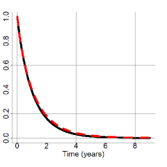
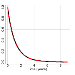
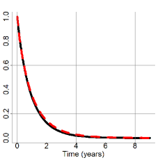
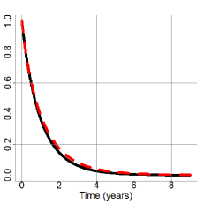
Figure 1: Posterior mean of the uncured survival function for individuals in the groups M-ST(on the top left), M-IFN (on the top right), W-ST (at the bottom left), and W-IFN (at the bottom right) computed with INLA (black solid line) and MCMC (red dashed line).

5.2 Bone marrow transplant study

Next, we consider the bone marrow transplant study dataset in Kersey et al. (1987) to illustrate our proposal for a Weibull AFTMC model. This study was undertaken to compare autologous and allogeneic marrow transplantation with regard to survival times of patients affected with lymphoblastic leukemia and poor prognosis. A total of $91$ patients were treated with high-doses of chemoradiotherapy and followed-up during a period between 1.4 to 5.0 years. Forty-six patients with a HLA-matched donor received a donor marrow (allogeneic graft) and 45 patients without a matched donor received their own marrow taken during remission and purged of leukemic cells with the use of monoclonal antibodies (autologous graft). The survival variable of interest was time to death, in days, which ranged from 11 to 1845 days. Data contain 22 right-censored observations and 69 uncensored. In general, times to death are longer for allogeneic transplant patients (sample median was 292 days) than for autologous patients (sample median was 112 days).

The main goal of the study was to compare both groups, autologous and allogeneic, with regard to the incidence and the latency models. Covariate information only contemplates the type of transplant and was incorporated in both terms of the cure model.

Incidence and latency model

The cure probability for individual $i$th corresponding to the incidence model was expressed in terms of a regression logistic model defined as

$$\mbox{logit}[\eta_{i}(\boldsymbol{\beta})]\,=\,\beta_{All,1}+\beta_{Aut,1}\,I_{Aut}(i),$$ (18)

where $\beta_{All,1}$ represents the effect of the reference category, to be an individual who has received an allogeneic transplant, and $I_{Aut}(i)$ is an indicator variable with value 1 whether individual $i$ has had an autologous graft.

Survival time for individual $i$ in the uncured subpopulation, $T_{ui}$, was modeled by means of a Weibull AFT model defined as

$$\mbox{log}(T_{ui}) =\beta_{All,2}+\beta_{Aut,2}\,I_{Aut}(i)+\sigma\,\epsilon_{i},$$ (19)

where now $\beta_{All,2}$ represents the effect of receiving an allogeneic graft, and $\beta_{Aut,1}$ the additional effect for having an autologous transplant.

The model is completed with the elicitation of a prior distribution for all parameters it contains. We assume prior independence and select vague normal distributions centered at zero and variance 1,000 for all the regression coefficients in the model except for $\alpha=1/\sigma$, for which a Ga(0.01, 0.01) distribution was selected.

Table 3: Summary of the INLA and MCMC approximate marginal posterior distributions: mean, standard deviation, 95$\%$ credible interval, and posterior probability that the subsequent parameter is positive.

		Parameter	Mean	Sd	95 $\%$CI	$P(\cdot>0)$
Incidence	INLA	$\beta_{All,1}$	-0.988	0.341	[-1.691,-0.351]	0.000
		$\beta_{Aut,1}$	-0.404	0.505	[-1.407,0.575]	0.211
	MCMC	$\beta_{All,1}$	-1.025	0.355	[-1.763,-0.367]	0.000
		$\beta_{Aut,1}$	-0.413	0.524	[-1.437,0.665]	0.203
Latency	INLA	$\beta_{All,2}$	-6.372	0.652	[-7.709,-5.131]	0.000
		$\beta_{Aut,2}$	0.759	0.262	[0.247, 1.277]	0.998
		$\alpha$	1.138	0.103	[0.941,1.343]	$-$
	MCMC	$\beta_{All,2}$	-6.305	0.631	[-7.572,-5.118]	0.000
		$\beta_{Aut,2}$	0.754	0.267	[0.238, 1.287]	1.000
		$\alpha$	1.124	0.101	[0.934,1.325]	$-$

Posterior inferences

Our algorithm configuration for this model included 20 burn-in iterations and other 180 for inference. In addition, the simulations were thinned by storing every 2nd draws in order to reduce autocorrelation in the saved sample. Convergence was evaluated by examining whether the conditional marginal log-likelihood estimates achieved stability during the iteration steps of our algorithm.

Table 4: Summary of the approximated INLA and MCMC posterior mean, standard deviation, and 95$\%$ credible interval of the cure proportion for allogeneic and autologous graft patients.

	Group	Mean	Sd	95 $\%$CI
INLA	All	0.286	0.067	[0.170,0.428]
	Aut	0.205	0.060	[0.107,0.342]
MCMC	All	0.270	0.067	[0.146,0.410]
	Aut	0.198	0.057	[0.094,0.319]

MCMC simulation was run considering three Markov chains with 200,000 iterations and a burn-in period with 40,000 iterations. The chains were thinned by storing every 400th iteration to reduce autocorrelation in the saved sample and avoid space computer problems. Convergence was also here assessed via the potential scale reduction factor and the effective number of independent simulation draw (Gelman and Rubin, 1992). As in the ECOG study, our proposed method here also needed less iterations than MCMC configuration to reach convergence and accurate results.

Table 3 shows the INLA and MCMC mean, standard deviation and 95$\%$ credible interval of the posterior distribution of the cure proportion for allogeneic and autologous transplant patients. INLA and MCMC results are very similar.

In the case of the estimation of derived quantities of interest, we proceed analogously to the ECOG study. We estimate the INLA and MCMC posterior distribution for the cure proportion for allogeneic and autologous transplant patients (Table 4) as well as the subsequent posterior mean of the uncured survival function (Figure 2). Outcomes also now present scarce differences and underline that allogeneic transplanted patients seem to have cure proportion levels higher than the ones for autologous patients, although we also appreciate a very broad degree of overlap.

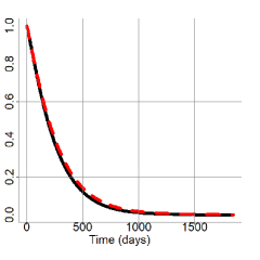
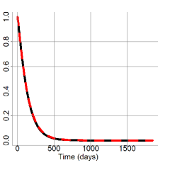
Figure 2: Posterior mean of the uncured survival function for Allogeneic (on the left) and Autologous (on the right) transplanted patients computed from INLA (black solid line) and MCMC (red dashed line)

6 Conclusions

This paper discussed an INLA approach for dealing with mixture cure models based on a general procedure by Bivand et al. (2014); Gómez-Rubio and Rue (2017); Gómez-Rubio (2018) that extends INLA to finite mixture models. We introduced latent indicators in the inferential process for classifying individuals in the cured and uncured subpopulations, and approximated the relevant posterior distribution via Gibbs sampling. In particular, we use modal Gibbs sampling (Gómez-Rubio, 2018) and INLA to fit the marginal posterior distribution of each relevant element given the latent indicator variable that identifies each individual in the cure or uncured population.

Two specific benchmark datasets from the field of medicine have been considered to illustrate our proposal. In both cases, the results support its viability and good performance, and almost entirely agree with the MCMC results. Remarkably, our proposal also shows other interesting properties such as the lower number of iterations to reach convergence and the convenient exploration of the parametric space of the latent indicators. Furthermore, the use of INLA to fit conditional models does not force the use of conjugate priors in the Gibbs sampler and avoids label switchings problems usually caused by symmetry in the likelihood function of the model parameters (Stephens, 2000).

On the other hand, MCMC provides, at the moment, slightly faster computational times and consequently, more research would be necessary to minimize computational efforts and storage requirements. Note that INLA estimates two complete models, incidence and latency, in each iteration. This leads to an important computational burden because two complete processes in each iteration were generated thus producing new temporary files and other secondary elements. So, if we limit the default outcomes provided by INLA and we define prior distributions based on the inferences from the previous iteration, computational savings could be achieved.

Declaration of Conflicting Interests: The authors declare that there is no conflict of interest.

Lázaro’s research was supported by a predoctoral FPU fellowship (FPU2013/02042) from the Spanish Ministry of Education, Culture and Sports. This paper was partially funded by grant MTM2016-77501-P from the Spanish Ministry of Economy and Competitiveness co-financed with FEDER funds, and a grant funded by Consejería de Educación, Cultura y Deportes (JCCM, Spain) and FEDER.

References

- Akerkar et al. (2010) Akerkar R, Martino S and Rue H (2010) Implementing approximate bayesian inference for survival analysis using integrated nested laplace approximations. Preprint Statistics, Norwegian University of Science and Technology 1: 1–38.
- Bivand et al. (2014) Bivand RS, Gómez-Rubio V and Rue H (2014) Approximate bayesian inference for spatial econometrics models. Spatial Statistics 9: 146 – 165.
- Caia et al. (2012) Caia C, Zoua Y, Pengb Y and Zhanga J (2012) smcure: An r-package for estimating semiparametric mixture cure models. Computer Methods and Programs in Biomedicine 108: 1255–1260.
- Christensen et al. (2011) Christensen R, Wesley J, Branscum A and Hanson TE (2011) Bayesian Ideas and Data Analysis: An Introduction for Scientists and Statisticians. Boca Raton: Boca Raton, Chapman & Hall/CRC Press.
- Cox (1972) Cox DR (1972) Regression models and life-tables. Journal of the Royal Statistical Society. Series B (Methodological) 34(2): 187–220.
- Diebolt and Robert (1994) Diebolt J and Robert CP (1994) Estimation of finite mixture distributions through bayesian sampling. Journal of the Royal Statistical Society. Series B (Methodological) : 363–375.
- Gelman and Rubin (1992) Gelman A and Rubin DB (1992) Inference from iterative simulation using multiple sequences. Statistical Science 7(4): 457 – 472.
- Gómez-Rubio (2018) Gómez-Rubio V (2018) Mixture model fitting using conditional models and modal Gibbs sampling. arXiv:1712.09566 .
- Gómez-Rubio and Rue (2017) Gómez-Rubio V and Rue H (2017) Markov chain monte carlo with the integrated nested laplace approximation. Statistics and Computing : 1–19.
- Hennerfeind et al. (2006) Hennerfeind A, Brezger A and Fahrmeir L (2006) Geoadditive survival models. Journal of the American Statistical Association 101(475): 1065–1075.
- Hurtado Rúa and Dey (2016) Hurtado Rúa SM and Dey DK (2016) A transformation class for spatio-temporal survival data with a cure fraction. Statistical Methods in Medical Research 25: 167–187.
- Ibrahim et al. (2001) Ibrahim JG, Chen MH and Sinha D (2001) Bayesian Survival Analysis. New York: Springer-Verlag.
- Kersey et al. (1987) Kersey JH, Weisdorf D, Nesbit ME, LeBien TW, Woods WG, McGlave PB, Kim T, Vallera DA, Goldman AI, Bostrom B et al. (1987) Comparison of Autologous and Allogeneic Bone Marrow Transplantation for Treatment of High-Risk Refractory Acute Lymphoblastic Leukemia. New England Journal of Medicine 317(8): 461–467.
- Kirkwood et al. (1996) Kirkwood JM, Strawderman MH, Ernstoff MS, Smith TJ, Borden EC and Blum RH (1996) Interferon alfa-2b adjuvant therapy of high-risk resected cutaneous melanoma: the Eastern Cooperative Oncology Group Trial EST 1684. Journal of Clinical Oncology 14(1): 7–17.
- Lambert et al. (2007) Lambert PC, Thompson JR, Weston CL and Dickman PW (2007) Estimating and modeling the cure fraction in population-based cancer survival analysis. Biostatistics 8(3): 576–594.
- Lázaro et al. (2018) Lázaro E, Armero C and Alvares D (2018) Bayesian regularization for flexible baseline hazard functions in Cox survival models. Submitted.
- Loredo (1989) Loredo TJ (1989) From Laplace To Supernova SN 1987A: Bayesian inference in astrophysics. Dordrecht: Kluwer Academic publishers, pp. 81–142.
- Loredo (1992) Loredo TJ (1992) Statistical challenges in modern astronomy. the promise of bayesian inference for astrophysics.
- Marin et al. (2005) Marin JM, Mengersen K and Robert CP (2005) Bayesian modelling and inference on mixtures of distributions, chapter 5. Elsevier, pp. 459–507.
- Martino et al. (2011) Martino S, Akerkar R and Rue H (2011) Approximate bayesian inference for survival models. Scandinavian Journal of Statistics 38(3): 514–528.
- Meeker (1987) Meeker WQ (1987) Limited failure population life tests: Application to integrated circuit reliability. Technometrics 29(1): 51–65.
- Peng and Taylor (2014) Peng Y and Taylor J (2014) Cure models, chapter 6. Boca Raton: Chapman and Hall, pp. 113–134.
- Plummer (2003) Plummer M (2003) JAGS: A Program for Analysis of Bayesian Graphical Models Using Gibbs sampling. In: Proceedings of the 3rd International Workshop on Distributed Statistical Computing.
- R Core Team (2014) R Core Team (2014) R: A Language and Environment for Statistical Computing. R Foundation for Statistical Computing, Vienna, Austria.
- Robinson (2014) Robinson M (2014) Mixture cure models: Simulation comparisons of methods in R and SAS. PhD Thesis, University of South Carolina.
- Rondeau et al. (2013) Rondeau V, Schaffner E, Corbière F, González JR and Mathoulin-Pélissier S (2013) Cure frailty models for survival data: Application to recurrences for breast cancer and to hospital readmissions for colorectal cancer. Statistical Methods in Medical Research 22: 243–260.
- Rue and Held (2005) Rue H and Held L (2005) Gaussian Markov Random Fields: Theory and Applications. Boca Raton: Chapman & Hall/CRC Press.
- Rue et al. (2009) Rue H, Martino S and Chopin N (2009) Approximate Bayesian inference for latent Gaussian models by using integrated nested Laplace approximations. Journal of the Royal Statistical Society: Series B (Methodological) 71(2): 319 – 392.
- Rue et al. (2017) Rue H, Riebler A, Sørbye SH, Illian JB, Simpson DP and Lindgren FK (2017) Bayesian computing with INLA: A review. Annual Review of Statistics and Its Application 4: 395 – 421.
- Schmidt and Witte (1989) Schmidt P and Witte AD (1989) Predicting criminal recidivism using ‘split population’ survival time models. Journal of Econometrics 40(1): 141 – 159.
- Sposto (2002) Sposto R (2002) Cure model analysis in cancer: an application to data from the children’s cancer group. Statistics in Medicine 21: 293–312.
- Stephens (2000) Stephens M (2000) Dealing with label switching in mixture models. Journal of the Royal Statistical Society: Series B (Statistical Methodology) 62(4): 795–809.