Partial least squares discriminant analysis: A dimensionality reduction method to classify hyperspectral data

Abstract

The recent development of more sophisticated spectroscopic methods allows acquisition of high dimensional datasets from which valuable information may be extracted using multivariate statistical analyses, such as dimensionality reduction and automatic classification (supervised and unsupervised). In this work, a supervised classification through a partial least squares discriminant analysis (PLS-DA) is performed on the hyperspectral data. The obtained results are compared with those obtained by the most commonly used classification approaches.

Piazzale Aldo Moro, 5 Rome (Italy) Sapienza University of Rome] Department of Statistical Science, Sapienza University, Rome (Italy) [University of Tuscia] Department for Innovation in Biological, Agro-food and Forest Systems,
University of Tuscia, Viterbo (Italy) [University of Tuscia] Department for Innovation in Biological, Agro-food and Forest Systems,
University of Tuscia, Viterbo (Italy)

1 Introduction

The recent development of more sophisticated spectroscopic approaches allows the acquisition of high dimensional datasets from which valuable information may be extracted via different multivariate statistical techniques. The high data dimensionality greatly enhances the informational content of the dataset and provides an additional opportunity for the current techniques for analyzing such data ¹. For example, automatic classification (clustering and/or classification) of data with similar features is an important problem in a variety of research areas such as biology, chemistry, and medicine ^{2, 3}. When the labels of the clusters are available, a supervised classification method is applied. Several classification techniques are available and described in the literature. However, data derived by spectroscopic detection represent a hard challenge for the researcher, who faces two crucial problems: data dimensionality larger than the observations, and high correlation levels among the variables (multicollinearity).
Usually, in order to solve these problems (i) a first data compression or reduction method, such as principal component analysis (PCA) is applied to shrink the number of variables; then, a range of discriminant analysis techniques is used to solve the classification problem, while (ii) in other cases, non-parametric classification approaches are used ^{1, 4, 5, 6, 7}.
In this work, the dataset consists of three different varieties of olives (Moraiolo, Dolce di Andria, and Nocellara Etnea) monitored during ripening up to harvest ⁸. Samples contained olives from 162 trees (54 for each variety), and 601 spectral detections (i.e., dimensions/variables) were performed using a portable near infrared acousto-optically tunable filter (NIR-AOTF) device in diffuse reflectance mode from 1100 nm to 2300 nm with an interval of 2. The use of NIRS on olive fruits and related products is already known; applications for the determination of oil and moisture content are now considered routine analyses in comparison with relatively new methodologies, such as nuclear magnetic resonance (NMR), or more traditional analytical determinations ^{9, 10, 11, 12}.
This paper is based on the use of partial least squares discriminant Analysis (PLS-DA). However, for comparison purposes, we also analyze the results obtained by other commonly used non-parametric classification models such as $K$-nearest neighbor (KNN), support vector machine (SVM) ^{13, 14, 15, 16}, and some variants of discriminant functions for sparse data as such as diagonal linear discriminant analysis (DLDA), maximum uncertainty linear discriminant analysis (MLDA), and shrunken linear discriminant analysis (SLDA). All the three regularization techniques compute linear discriminant functions ^{17, 18, 19, 20, 21, 22}.
PLS-DA is a dimensionality reduction technique, a variant of partial least squares regression (PLS-R) that is used when the response variable is categorical. It is a compromise between the usual discriminant analysis and a discriminant analysis on the principal components of the predictor variables. In particular, PLS-DA instead of finding hyperplanes of maximum variance between the response and independent variables finds a linear regression model by projecting the predicted variables and the observed variables into a new space. PLS-DA can provide good insight into the causes of discrimination via weights and loadings, which gives it a unique role in exploratory data analysis, for example in metabolomics via visualization of significant variables such as metabolites or spectroscopic peaks ^{23, 24, 25}.
The paper is structured as follows: in section 2 we provide a background on the most commonly used non-parametric statistical methodologies to solve the classification problem of sparse data (i.e., KNN and SVM) and an overview of different classifiers derived from linear discriminant analysis (LDA), in section 3 we focus on the PLS-DA model with a deeper examination of the PLS algorithm, in section 4 we show a comparison of the results obtained by the application of PLS-DA and those obtained by the other common classification methods, and finally in section 5 we provide some suggestions and ideas for future research.

2 Background

In this section, we present a brief overview of different classifiers that have been highly successful in handling high dimensional data classification problems, starting with popular methods such as $K$-nearest neighbor (KNN) and support vector machines (SVM) ^{21, 26} and variants of discriminant functions for sparse data ¹⁸. We also examine dimensionality reduction techniques and their integration with some existing algorithms (i.e., partial least squares discriminant analysis (PLS-DA)) ^{23, 24}.

2.1 $K$-nearest neighbor (KNN)

The KNN method was first introduced by Fix and Hodges ²⁷ based on the need to perform discriminant analysis when reliable parametric estimates of probability densities are unknown or difficult to determine. In this method, a distance measure (e.g., Euclidean) is assigned between all points in the data. The data points, $K$-closest neighbors (where $K$ is the number of neighbors), are then found by analyzing a distance matrix. The $K$-closest data points are then found and analyzed in order to determine which class label is the most common among the set. Finally, the most common class label is then assigned to the data point being analyzed ¹³.
The KNN classifier is commonly based on the Euclidean distance between a test sample and the specified training samples. Formally, let $\mathbf{x}_{i}$ be an input sample with $J$ features ($\mathbf{x}_{i,1},\dots,\mathbf{x}_{i,J}$), and $n$ be the total number of input samples ($i=1,\dots,n$). The Euclidean distance between sample $\mathbf{x}_{i}$ and $\mathbf{x}_{l}$ ($l=1,\dots,n$) is defined as

$$d(\mathbf{x}_{i},\mathbf{x}_{l})=\sqrt{(\mathbf{x}_{i,1}-\mathbf{x}_{l,1})^{2}+\dots+(\mathbf{x}_{i,J}-\mathbf{x}_{l,J})^{2}}.$$ (1)

Using the latter characteristic, the KNN classification rule is to assign to a test sample the majority category label of its $K$ nearest training samples. In other words, $K$ is usually chosen to be odd, so as to avoid ties. The $K=1$ rule is generally called the 1-nearest-neighbor classification rule.
Then, let $\mathbf{x}_{i}$ be a training sample and $\mathbf{x}_{i}^{*}$ be a test sample, and let $\omega$ be the true class of a training sample and $\hat{\omega}$ be the predicted class for a test sample ($\omega,\hat{\omega}=\,\dots,\Omega$), where $\Omega$ is the total number of classes. During the training process, only the true class $\omega$ of each training sample to train the classifier is used, while during testing the class $\hat{\omega}$ of each test sample is predicted. With 1-nearest neighbor rule, the predicted class of test sample $\mathbf{x}_{i}^{*}$ is set equal to the true class $\omega$ of its nearest neighbor, where $\mathbf{z}_{i}$ is a nearest neighbor to $\mathbf{x}_{i}^{*}$ if the distance

$$d(\mathbf{z}_{i},\mathbf{x}_{i}^{*})=\min_{j}\{d(\mathbf{z}_{j},\mathbf{x}_{i}^{*})\}.$$ (2)

For the $K$-nearest neighbors rule, the predicted class of test sample $\mathbf{x}_{i}^{*}$ is set equal to the most frequent true class among the $K$ nearest training samples.

2.2 Support vector machine (SVM)

The SVM approach was developed by Vapnik ^{28, 29}. Synthetically, SVM is a linear method in a very high dimensional feature space that is nonlinearly related to the input space. The method maps input vectors to a higher dimensional space where a maximal separating hyperplane is constructed ¹⁶. Two parallel hyperplanes are constructed on each side of the hyperplane that separates the data and maximizes the distance between the two parallel hyperplanes. An assumption is made that the larger the margin or distance between these parallel hyperplanes, the better the generalization error of the classifier will be.
SVM was initially designed for binary classification. To extend SVM to the multi-class scenario, a number of classification models were proposed ³⁰. Formally, given training vectors $\mathbf{x}_{i}\in\Re^{J}$, $i=1,\dots,n^{*}$, in two classes, and the label vector $\mathbf{Y}\in\{-1,1\}^{n^{*}}$ (where $n^{*}$ in the size of the training samples), the support vector technique requires the solution of the following optimization problem:

$$\begin{split}\min_{\mathbf{w}\in H,b\in\Re,\xi_{i}\in\Re}&\frac{1}{2}\mathbf{w}^{T}\mathbf{w}+C\sum_{i=1}^{n^{*}}\xi_{i},\\ subject\>\>to\quad&y_{i}(\mathbf{w}^{T}\varphi(\mathbf{x}_{i})+b)\geq 1-\xi_{i}\\ \quad\quad\quad\quad\quad\quad&\xi_{i}\geq 0,\quad i=1,\dots,n^{*},\end{split}$$ (3)

where $\mathbf{w}\in\Re^{J}$ is the weights vector, $C\in\Re_{+}$ is the regularization constant, and the mapping function $\varphi$ projects the training data into a suitable feature space $H$.
For a $K$-class problem, many methods use a single objective function for training all $K$-binary SVMs simultaneously and maximize the margins from each class to the remaining ones ^{30, 31}. An example is the formulation proposed by Weston and Watkins ³¹. Given a labeled training set represented by $\{(\mathbf{x}_{1},y_{1}),\dots,(\mathbf{x}_{n^{*}},y_{n^{*}})\}$, where $\mathbf{x}_{i}\in\Re^{J}$ and $y_{i}\in\{1,\dots,K\}$, this formulation is given as follows:

$$\begin{split}\min_{\mathbf{w}_{k}\in H,b\in\Re^{K},\xi\in\Re^{n^{*}\times K}}&\frac{1}{2}\sum_{k=1}^{K}\mathbf{w}_{k}^{T}\mathbf{w}_{k}+C\sum_{i=1}^{n^{*}}\sum_{t\neq y_{i}}\xi_{i,t},\\ subject\>\>to\quad&\mathbf{w}_{y_{i}}^{T}\varphi(\mathbf{x}_{i})+b_{y_{i}})\geq\mathbf{w}_{t}^{T}\varphi(\mathbf{x}_{i})+b_{t}+2-\xi_{i,t},\\ \quad\quad\quad\quad\quad\quad&\xi_{i,t}\geq 0,\quad i=1,\dots,n^{*},\quad t\in\{1,\dots,K\}.\end{split}$$ (4)

The resulting decision function is given in Equation 5 ³⁰.

$$\operatorname*{argmax}_{k}f_{m}(\mathbf{x})=\operatorname*{argmax}_{k}(\mathbf{w}_{k}^{T}\varphi(\mathbf{x}_{i})+b_{k}).$$ (5)

2.3 Discriminant analysis functions

In this section we present a comprehensive overview of different classifiers derived by Linear Discriminant Analysis (LDA), and that have been highly successful in handling high dimensional data classification problems: Diagonal Linear Discriminant Analysis (DLDA), Maximum uncertainty Linear Discriminant Analysis (MLDA), and Shrunken Linear Discriminant Analysis (SLDA). All the three regularization techniques compute Linear Discriminant Functions, by default after a preliminary variable selection step, based on alternative estimators of a within-groups covariance matrix that leads to reliable allocation rules in problems where the number of selected variables is close to, or larger than, the number of available observations.
The main purpose of discriminant analysis is to assign an unknown subject to one of $K$ classes on the basis of a multivariate observation $x=(x_{1},\dots,x_{J})^{\prime}$, where $J$ is the number of variables. The standard LDA procedure does not assume that the populations of the distinct groups are normally distributed, but it assumes implicitly that the true covariance matrices of each class are equal because the same within-class covariance matrix is used for all the classes considered ^{19, 32}. Formally, let $\mathbf{S}_{b}$ be the between-class covariance matrix defined as

$$\mathbf{S}_{b}=\sum_{k=1}^{K}n_{k}(\bar{x}_{k}-\bar{x})(\bar{x}_{k}-\bar{x})^{T},$$ (6)

and let $\mathbf{S}_{w}$ be the within-class covariance matrix defined as

$$\mathbf{S}_{w}=\sum_{k=1}^{K}(n_{k}-1)\mathbf{S}_{k}=\sum_{k=1}^{K}\sum_{i=1}^{n_{k}}(\bar{x}_{k,i}-\bar{x}_{k})(\bar{x}_{k,i}-\bar{x}_{k})^{T},$$ (7)

where $x_{k,i}$ is the $J$-dimensional pattern $i$ from the $k$-th class, $n_{k}$ is the number of training patterns from the $k$-th class, and $K$ is the total number of classes (or groups) considered. The vector $\bar{x}_{k}$ and matrix $\mathbf{S}_{k}$ are respectively the unbiased sample mean and sample covariance matrix of the $k$-th class, while the vector $\bar{x}$ is the overall unbiased sample mean given by

$$\bar{x}=\frac{1}{n}\sum_{k=1}^{K}n_{k}\bar{x}_{k}=\frac{1}{n}\sum_{k=1}^{K}\sum_{i=1}^{n_{k}}x_{k,i},$$ (8)

where $n$ is the total number of samples $n=n_{1}+\dots+n_{K}$.
Then, the main objective of LDA is to find a projection matrix (here defined as $\mathbf{P}_{LDA}$) that maximizes the ratio of the determinant of the between-class scatter matrix to the determinant of the within-class scatter matrix (Fisher’s criterion). Formally,

$$\mathbf{P}_{LDA}=\operatorname*{argmax}_{\mathbf{P}}\frac{det\left(\mathbf{P}^{T}\mathbf{S}_{b}\mathbf{P}\right)}{det\left(\mathbf{P}^{T}\mathbf{S}_{w}\mathbf{P}\right)}.$$ (9)

It has been shown ³³ that Equation (9) is in fact the solution of the following eigenvector system problem:

$$\mathbf{S}_{b}\mathbf{P}-\mathbf{S}_{w}\mathbf{P}\Lambda=0.$$ (10)

Note that by multiplying both sides by $\mathbf{S}_{w}^{-1}$, Equation (10) can be rewritten as

$$\begin{split}&\mathbf{S}_{w}^{-1}\mathbf{S}_{b}\mathbf{P}-\mathbf{S}_{w}^{-1}\mathbf{S}_{w}\mathbf{P}\Lambda=0\\ &\mathbf{S}_{w}^{-1}\mathbf{S}_{b}\mathbf{P}-\mathbf{P}\Lambda=0\\ &(\mathbf{S}_{w}^{-1}\mathbf{S}_{b})\mathbf{P}=\mathbf{P}\Lambda,\end{split}$$ (11)

where $\mathbf{P}$ and $\Lambda$ are respectively the eigenvector and eigenvalue matrices of the $\mathbf{S}_{w}^{-1}\mathbf{S}_{b}$ matrix. These eigenvectors are primarily used for dimensionality reduction, as in principal component analysis (PCA) ³⁴.
However, the performance of the standard LDA can be seriously degraded if there are only a limited number of total training observations $n$ compared to the number of dimensions of the feature space $J$. In this context, in fact the $\mathbf{S}_{w}$ matrix becomes singular. To solve this problem, Yu and Yang ^{19, 35} have developed a direct LDA algorithm (called DLDA) for high dimensional data with application to face recognition that diagonalizes simultaneously the two symmetric matrices $\mathbf{S}_{w}$ and $\mathbf{S}_{b}$. The idea of DLDA is to discard the null space of $\mathbf{S}_{b}$ by diagonalizing $\mathbf{S}_{b}$ first and then diagonalizing $\mathbf{S}_{w}$.
The following steps describe the DLDA algorithm for calculating the projection matrix $\mathbf{P}_{DLDA}$:
1. diagonalize $\mathbf{S}_{b}$, that is, calculate the eigenvector matrix $\mathbf{V}$ such that $\mathbf{V}^{T}\mathbf{S}_{b}\mathbf{V}=\Lambda$;
2. let $\mathbf{Y}$ be a sub-matrix with the first $m$ columns of $\mathbf{V}$ corresponding to the $\mathbf{S}_{b}$ largest eigenvalues, where $m\leq rank(\mathbf{S}_{b})$. Calculate the diagonal $m\times m$ sub-matrix of the eigenvalues of $\Lambda$ as $\mathbf{D}_{b}=\mathbf{Y}^{T}\mathbf{S}_{b}\mathbf{Y}$;
3. let $\mathbf{Z}=\mathbf{YD}_{b}^{-1/2}$ be a whitening transformation of $\mathbf{S}_{b}$ that reduces its dimensionality from $J$ to $m$ (where $\mathbf{Z}^{T}\mathbf{S}_{b}\mathbf{Z}=\mathbf{I}$). Diagonalize $\mathbf{Z}^{T}\mathbf{S}_{w}\mathbf{Z}$, that is, compute $\mathbf{U}$ and $\mathbf{D}_{w}$ such that $\mathbf{U}^{T}(\mathbf{Z}^{T}\mathbf{S}_{w}\mathbf{Z})\mathbf{U}=\mathbf{D}_{w}$;
4. calculate the projection matrix as $\mathbf{P}_{DLDA}=\mathbf{D}_{w}^{-1/2}\mathbf{U}^{T}\mathbf{Z}^{T}$.
Note that by replacing the between-class covariance matrix $\mathbf{S}_{b}$ with total covariance matrix $\mathbf{S}_{T}$ ($\mathbf{S}_{T}=\mathbf{S}_{b}+\mathbf{S}_{w}$), the first two steps of the algorithm become exactly the PCA dimensionality reduction technique ³⁵.
Two other approaches commonly used to avoid both the critical singularity and instability issues of the within-class covariance matrix $\mathbf{S}_{w}$ are SLDA and the MLDA ¹⁹. Firstly, it is important to note that the within-class covariance matrix $\mathbf{S}_{w}$ is essentially the standard pooled covariance matrix $\mathbf{S}_{p}$ multiplied by the scalar $(n-K)$. Then,

$$\mathbf{S}_{w}=\sum_{k=1}^{K}(n_{k}-1)\mathbf{S}_{k}=(n-K)\mathbf{S}_{p}.$$ (12)

From this property, the key idea of some regularization proposals of LDA ^{22, 36, 37} is to replace the pooled covariance matrix $\mathbf{S}_{p}$ of the within-class covariance matrix $\mathbf{S}_{w}$ with the following convex combination:

$$\hat{\mathbf{S}}_{p}(\gamma)=(1-\gamma)\mathbf{S}_{p}+\gamma\bar{\lambda}\mathbf{I},$$ (13)

where $\gamma\in[0,1]$ is the shrinkage parameter, which can be selected to maximize the leave-one-out classification accuracy ³⁸, $\mathbf{I}$ is the identity matrix, and $\bar{\lambda}=J^{-1}\sum_{j=1}^{J}\lambda_{j}$ is the average eigenvalue, which can be written as $J^{-1}trace(\mathbf{S}_{p})$. This regularization approach, called SLDA, would have the effect of decreasing the larger eigenvalues and increasing the smaller ones, thereby counteracting the biasing inherent in eigenvalue sample-based estimation ^{19, 17}.
In contrast, in the MLDA method a multiple of the identity matrix determined by selecting the largest dispersions regarding the $\mathbf{S}_{p}$ average eigenvalue is used. In particular, if we replace the pooled covariance matrix $\mathbf{S}_{p}$ of the covariance matrix $\mathbf{S}_{w}$ (shown in Equation (12)) with a covariance estimate of the form $\hat{\mathbf{S}}_{p}(\delta)=\mathbf{S}_{p}+\delta\mathbf{I}$ (where $\delta\geq 0$ is an identity matrix multiplier), then the eigen-decomposition of a combination of the covariance matrix $\mathbf{S}_{p}$ and the $J\times J$ identity matrix $\mathbf{I}$ can be written as

$$\begin{split}\hat{\mathbf{S}}_{p}(\delta)&=\mathbf{S}_{p}+\delta\mathbf{I}\\ &=\sum_{j=1}^{r}\lambda_{j}\phi_{j}(\phi_{j})^{T}+\delta\sum_{j=1}^{J}\phi_{j}(\phi_{j})^{T}\\ &=\sum_{j=1}^{r}(\lambda_{j}+\delta)\phi_{j}(\phi_{j})^{T}+\sum_{j=1}^{J}\delta\phi_{j}(\phi_{j})^{T},\end{split}$$ (14)

where $r$ is the rank of $\mathbf{S}_{p}$ (note that $r\leq J$), $\lambda_{j}$ is the $j$-th eigenvalue of $\mathbf{S}_{p}$, $\phi_{j}$ is the $j$-th corresponding eigenvector, and $\delta$ is the identity matrix multiplier previously defined. In fact, in Equation (14) the identity matrix is defined as $\mathbf{I}=\sum_{j=1}^{J}\phi_{j}(\phi_{j})^{T}$. Now, given the convex combination shown in Equation (13), the eigen-decomposition can be written as

$$\begin{split}\hat{\mathbf{S}}_{p}(\gamma)&=(1-\gamma)\mathbf{S}_{p}+\gamma\bar{\lambda}\mathbf{I}\\ &=(1-\gamma)\sum_{j=1}^{r}\lambda_{j}\phi_{j}(\phi_{j})^{T}+\gamma\sum_{j=1}^{J}\bar{\lambda}\phi_{j}(\phi_{j})^{T}.\end{split}$$ (15)

The steps of the MLDA algorithm are shown follows:
1. Find the $\Phi$ eigenvectors matrix and $\Lambda$ eigenvalues matrix ff $\mathbf{S}_{p}$, where $\mathbf{S}_{p}=(n-K)\mathbf{S}_{w}$ (from Equation (12));
2. Calculate $\mathbf{S}_{p}$ average eigenvalues as $J^{-1}trace(\mathbf{S}_{p})$;
3. Construct a new matrix of eigenvalues based on the following largest dispersion values :

$$\Lambda^{*}=diag\left[max(\lambda_{1},\bar{\lambda}),\dots,max(\lambda_{J},\bar{\lambda})\right];$$

4. Define the revised within-class covariance matrix:

$$\mathbf{S}_{w}^{*}=(n-K)\mathbf{S}_{p}^{*}=(n-K)(\Phi\Lambda^{*}\Phi^{T}).$$

Then, the MLDA approach is based on replacing $\mathbf{S}_{w}$ with $\mathbf{S}_{w}^{*}$ in the Fisher’s criterion formula described in Equation (9).

3 Partial Least Squares Discriminant Analysis (PLS-DA)

Multivariate regression methods like principal component regression (PCR) and partial least squares regression (PLS-R) enjoy large popularity in a wide range of fields and are mostly used in situations where there are many, possibly correlated, predictor variables and relatively few samples, a situation that is common, especially in chemistry, where developments in spectroscopy since the seventies have revolutionized chemical analysis ^{25, 39}. In fact, the origin of PLSR lies in chemistry ^{25, 40, 41}.
In practice, there are not many differences between the use of PCR and PLS-R; in most situations, the methods achieve similar prediction accuracies. Note that with the same number of latent variables, PLS-R will cover more of the variation in $\mathbf{Y}$ and PCR will cover more of the variation in $\mathbf{X}$. ²⁵.
Partial least squares discriminant Analysis (PLS-DA) is a variant of PLS-R that can be used when the response variable $\mathbf{Y}$ is categorical. Under certain circumstances, PLS-DA provides the same results as the classical approach of Euclidean distance to centroids (EDC) ⁴² and under other circumstances, the same as that of linear discriminant analysis (LDA) ⁴³. However, in different contexts this technique is specially suited to deal with models with many more predictors than observations and with multicollinearity, two of the main problems encountered when analyzing hyperspectral detection data ³⁹.

3.1 Model and algorithm

PLS-DA is derived from PLS-R, where the response vector $\mathbf{Y}$ assumes discrete values. In the usual multiple linear regression model (MLR) approach we have

$$\mathbf{Y}=\mathbf{XB}+\mathbf{F},$$ (16)

where $\mathbf{X}$ is the $n\times J$ data matrix, $\mathbf{B}$ is the $J\times 1$ regression coefficients matrix, $\mathbf{F}$ is the $n\times 1$ error vector, and $\mathbf{Y}$ is the $n\times 1$ response variable vector. In this approach, the least squares solution is given by $\mathbf{B}=(\mathbf{X^{T}X})^{-1}\mathbf{X^{T}Y}$.
In many cases, the problem is the singularity of the $\mathbf{X^{T}X}$ matrix (e.g., when there are multicollinearity problems in the data or the number of predictors is larger than the number of observations). Both PLS-R and PLS-DA solve this problem by decomposing the data matrix $\mathbf{X}$ into $P$ orthogonal scores $\mathbf{T}$ ($n\times P$) and loadings matrix $\mathbf{P}$ ($J\times P$), and the response vector $\mathbf{Y}$ into $P$ orthogonal scores $\mathbf{T}$ ($n\times P$) and loadings matrix $\mathbf{Q}$ ($1\times P$). Then, let $\mathbf{E}$ and $\mathbf{F}$ be the $n\times J$ and $n\times 1$ error matrices associated with the data matrix $\mathbf{X}$ and response vector $Y$, respectively. There are two fundamental equations in the PLS-DA model:

$$\begin{split}&\mathbf{X}=\mathbf{TP^{T}}+\mathbf{E}\\ &\mathbf{Y}=\mathbf{TQ^{T}}+\mathbf{F}.\end{split}$$ (17)

Now, if we define a $J\times P$ weights matrix $\mathbf{W}$, we can write the scores matrix as

$$\mathbf{T}=\mathbf{XW}(\mathbf{P^{T}W})^{-1},$$ (18)

and by substituting it into the PLS-DA model, we obtain

$$\mathbf{Y}=\mathbf{XW}(\mathbf{P^{T}W})^{-1}\mathbf{Q^{T}}+\mathbf{F},$$ (19)

where the regression coefficient vector $\mathbf{B}$ is given by

$$\hat{\mathbf{B}}=\mathbf{W}(\mathbf{P^{T}W})^{-1}\mathbf{Q^{T}}.$$ (20)

In this way, an unknown sample value of $\mathbf{Y}$ can be predicted by $\hat{\mathbf{Y}}=\mathbf{X}\hat{\mathbf{B}}$, i.e. $\hat{\mathbf{Y}}=\mathbf{X}\mathbf{W}(\mathbf{P^{T}W})^{-1}\mathbf{Q^{T}}$. The PLS-DA algorithm estimates the matrices $\mathbf{W}$, $\mathbf{T}$, $\mathbf{P}$, and $\mathbf{Q}$ through the following steps ²⁴.

1:  Fixed $P$, initialize the residuals matrices $\mathbf{E_{0}}=\mathbf{X}$ and $\mathbf{F_{0}}=\mathbf{Y}$;

2:  for $p=1$ to $P$ do

3:     Calculate PLS weights vector$\mathbf{W_{p}}=\mathbf{E_{0}^{T}}\mathbf{F_{0}}$;

4:     Calculate and normalize scores vector$\mathbf{T_{p}}=\mathbf{E_{0}}\mathbf{W_{p}}(\mathbf{W_{p}^{T}E_{0}^{T}E_{0}W_{p}})^{-1/2}$ ;

5:     Calculate the $\mathbf{X}$ loadings vector$\mathbf{P_{p}}=\mathbf{E_{0}^{T}T_{p}}$;

6:     Calculate $\mathbf{Y}$ loading$\mathbf{Q_{p}}=\mathbf{F_{0}^{T}T_{p}}$;

7:     Update the $\mathbf{X}$ residuals vector$\mathbf{E_{0}}=\mathbf{E_{0}}-\mathbf{T_{p}P_{p}^{T}}$;

8:     Update the $\mathbf{Y}$ residuals vector$\mathbf{F_{0}}=\mathbf{F_{0}}-\mathbf{T_{p}Q_{p}^{T}}$;

9:  end for

10:  Obtain output matrices $\mathbf{W}$, $\mathbf{T}$, $\mathbf{P}$, $\mathbf{Q}$.

Algorithm 1 Partial Least Squares

4 Application to real data

In this section we show an application of the method to real data. In particular, we compare the results obtained by partial least squares discriminant analysis (PLS-DA) and the other classification techniques discussed in Section 2.

4.1 Dataset

The dataset consists of 162 drupes of olives harvested in 2010 belonging to three different cultivars (response variable): 54 Dolce di Andria (low phenolic concentration), 54 Moraiolo (high phenolic concentration), and 54 Nocellara Etnea (medium phenolic concentration). Spectral detection is performed using a portable NIR device (diffuse reflectance mode) in the 1100–2300 nm wavelength range, with 2 nm wavelength increments (601 observed variables) ⁸.

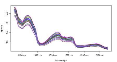
Figure 1: Representation of spectral detections performed on the 1100–2300 nm wavelength range

4.2 Principal results

In order to evaluate the prediction capability of the model, the entire data set has been randomly divided into a training set composed of 111 balanced observations (i.e., about 70% of the entire sample, with each class composed of 37 elements), and a test set (drawn from the sample) composed of 51 observations balanced across the three cultivars (i.e., about 30% of the entire sample and each class composed by 17 elements) ⁴⁴.
The first step of the analysis consists in selecting the optimal number of components $P$, i.e., the number of latent scores to consider for representing the original variable space. For this purpose, the latent subspace must explain the largest possible proportion of the total variance to guarantee the best model estimation. Table 1 shows the proportion of the total variance explained by the first five components identified by PLS-DA.

Table 1: Cumulative proportion of the total variance explained by the first five components (percent values)

	Comp. 1	Comp. 2	Comp. 3	Comp. 4	Comp. 5
Exp.Variance	61.152	35.589	0.892	0.982	1.167
Cum. Sum	61.152	96.741	97.633	98.615	99.782

The table shows that the first two components explain about 97% of the total variance, and only the first two latent scores have a significant contribution. Thus, it seems that the best latent subspace is represented by the plane composed of the first two identified components. However, in order to guarantee the best model estimate, it is also useful to understand its prediction quality with regard to the different subspace dimensions. In other words, the selection of the optimal number of components must be related to some criterion that ensures the maximum prediction quality of the estimated model. In this paper, we propose the maximization of the chi-squared test applied on the comparison between the real training partition and the predicted training partition ⁴⁵. Figure 2 represents the chi-squared values for different numbers of components (i.e., from 2 to 10 selected components).

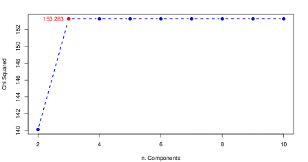
Figure 2: Chi-squared values with respect to different choices of components number

In the scree-plot shown in Figure 2, the chi-squared criterion suggests $P=3$ as the optimal number of components, where the maximum value of the chi-squared test is equal to 153.28. Then, we can select three components to estimate the model, but we can use the plane composed of the first two latent scores to represent the estimated groups (i.e., using 97% of the total information in the data).
Figure 3 shows the loadings distributions and the squared of the loadings distributions of the three $\mathbf{X}$s’ latent scores, measured on all the observed variables (i.e., on the 1100–2300 nm wavelength range).

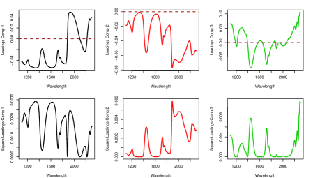
Figure 3: The loadings distributions (top) and squared loadings distributions (bottom) of the three latent scores measured on all the observed variables

By observing the behavior of the loadings, we can say that the wavelengths from about 1100 nm to about 1500 nm have a high negative contribution to the first two components, while they have a positive contribution to the third component; the wavelengths from about 1500 nm to about 1900 nm have a negative contribution to all three components, with the largest contribution to the first component; finally, the wavelengths from about 1900 nm to about 2300 nm have a positive contribution to both the first and the third component, while they have a negative contribution to the second component.
Now, we compare the classification results obtained by the PLS-DA procedure with results obtained by other classifiers, including $K$-nearest neighbor (KNN, $R$ package:⁴⁶), support vector machine (SVM, $R$ package ⁴⁷), diagonal linear discriminant analysis (DLDA, $R$ package ⁴⁸), maximum uncertainty linear discriminant analysis (MLDA, $R$ package ⁴⁸), and shrunken linear discriminant analysis (SLDA, $R$ package ⁴⁸). For the measurement of the model prediction quality, we have used mis classification rate (MIS), adjusted Rand Index (ARI) ⁴⁹, and the chi-squared test ($\chi^{2}$). The three measures have been computed on the comparison between the real data partition and the predicted partition.
Formally, let Table 2 (here called $T$) be the $K\times K$ confusion matrix where the real data partition and the predicted partition have been compared, $MIS=1-n^{-1}\left[\sum_{r=1}^{R}\sum_{=1}^{C}n_{rc}\right]$, while $ARI=\frac{\sum_{r=1}^{R}\sum_{=1}^{C}\binom{n_{rc}}{2}-\binom{n}{2}^{-1}\sum_{r=1}^{R}\binom{n_{r.}}{2}\sum_{c=1}^{C}\binom{n_{.c}}{2}}{\frac{1}{2}\left[\sum_{r=1}^{R}\binom{n_{r.}}{2}+\sum_{c=1}^{C}\binom{n_{.c}}{2}\right]-\binom{n}{2}^{-1}\sum_{r=1}^{R}\binom{n_{r.}}{2}\sum_{c=1}^{C}\binom{n_{.c}}{2}}$.

Table 2: An example of a confusion matrix between the real data partition and the predicted partition

	Predicted partition
		$P_{1}$	$\cdots$	$P_{C}$
Real partition	$R_{1}$	$n_{11}$	$\cdots$	$n_{1C}$	$n_{1\cdot}$
	$\vdots$	$\vdots$	$\ddots$	$\vdots$	$\vdots$
	$R_{R}$	$n_{R1}$	$\cdots$	$n_{RC}$	$n_{R\cdot}$
		$n_{\cdot 1}$	$\cdots$	$n_{\cdot C}$	$n$

Table 3 shows the results for the quality of the model predictions obtained on the training set and the test set.

Table 3: Model prediction quality computed on the training set and the test set

	Training set			Test set
	MIS	ARI	$\chi^{2}$	MIS	ARI	$\chi^{2}$
PLS-DA	0.002	0.880	153.283	0.008	0.710	77.182
KNN	0.027	0.755	151.744	0.157	0.625	65.294
SVM	0.072	0.797	152.688	0.137	0.615	69.750
DLDA	0.241	0.368	101.599	0.255	0.351	46.714
MLDA	0.078	0.734	149.577	0.010	0.699	72.311
SLDA	0.005	0.712	150.456	0.011	0.702	75.899

From the results, we can see that PLS-DA has the best performance on both the training set and the test set. This result is confirmed by the representation of the predicted partition on the first two $\mathbf{X}$s’ latent scores (i.e., on about 97% of the total data variance) as shown in Figures 4 and 5 (training set and the test set, respectively). In fact, we can see that, with respect to the other studied methodologies, PLS-DA identifies more homogeneous and better-separated classes.

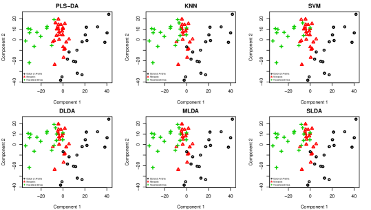
Figure 4: Representation of the predicted partition on the first two latent scores (training set)

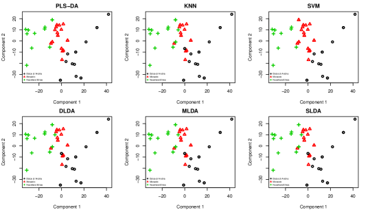
Figure 5: Representation of the predicted partition on the first two latent scores (test set)

5 Concluding remarks

Data acquired via spectroscopic detection represent a hard challenge for researchers, who face two crucial problems: data dimensionality larger than the number of observations, and high correlation levels among the variables. In this paper, partial least squares discriminant analysis (PLS-DA) modeling was proposed as a method to classify hyperspectral data. The results obtained on real data show that PLS-DA identifies classes that are more homogeneous and better-separated than other commonly used methods, such as non-parametric classifiers and other discriminant functions.
Moreover, we think that PLS-DA is a very important tool in terms of dimensionality reduction, as it can maximize the total variance of data using just a few components (i.e., the $\mathbf{X}$s’ latent scores). In fact, the PLS-DA components enable a good graphical representation of the partition, which is not possible with other approaches.
In future studies, the use of PLS for unsupervised classification could be a useful tool when both the number and structure of the groups are unknown.

References

- Jimenez and Landgrebe 1998 Jimenez, L. O.; Landgrebe, D. A. Supervised classification in high-dimensional space: geometrical, statistical, and asymptotical properties of multivariate data. IEEE Transactions on Systems, Man, and Cybernetics, Part C (Applications and Reviews) 1998, 28, 39–54
- Hardy et al. 2006 others,, et al. Fine-scale genetic structure and gene dispersal inferences in 10 Neotropical tree species. Molecular ecology 2006, 15, 559–571
- Galvan et al. 2006 others,, et al. Reversal of Alzheimer’s-like pathology and behavior in human APP transgenic mice by mutation of Asp664. Proceedings of the National Academy of Sciences 2006, 103, 7130–7135
- Agrawal et al. 1998 Agrawal, R.; Gehrke, J.; Gunopulos, D.; Raghavan, P. Automatic subspace clustering of high dimensional data for data mining applications; ACM, 1998; Vol. 27
- Bühlmann and Van De Geer 2011 Bühlmann, P.; Van De Geer, S. Statistics for high-dimensional data: methods, theory and applications; Springer Science & Business Media, 2011
- Kriegel et al. 2009 Kriegel, H.-P.; Kröger, P.; Zimek, A. Clustering high-dimensional data: A survey on subspace clustering, pattern-based clustering, and correlation clustering. ACM Transactions on Knowledge Discovery from Data (TKDD) 2009, 3, 1
- Ding and Gentleman 2005 Ding, B.; Gentleman, R. Classification using generalized partial least squares. Journal of Computational and Graphical Statistics 2005, 14, 280–298
- Bellincontro et al. 2012 Bellincontro, A.; Taticchi, A.; Servili, M.; Esposto, S.; Farinelli, D.; Mencarelli, F. Feasible application of a portable NIR-AOTF tool for on-field prediction of phenolic compounds during the ripening of olives for oil production. Journal of agricultural and food chemistry 2012, 60, 2665–2673
- Garcia et al. 1996 Garcia, J. M.; Seller, S.; Perez-Camino, M. C. Influence of fruit ripening on olive oil quality. Journal of agricultural and food chemistry 1996, 44, 3516–3520
- Gallardo et al. 2005 Gallardo, L.; Osorio, E.; Sanchez, J. Application of near infrared spectroscopy (NIRS) for the real-time determination of moisture and fat contents in olive pastes and wastes of oil extraction. Alimentación Equipos y Tecnologia 2005, 24, 85–89
- León et al. 2004 León, L.; Garrido-Varo, A.; Downey, G. Parent and harvest year effects on near-infrared reflectance spectroscopic analysis of olive (Olea europaea L.) fruit traits. Journal of agricultural and food chemistry 2004, 52, 4957–4962
- Cayuela and Camino 2010 Cayuela, J. A.; Camino, M. d. C. P. Prediction of quality of intact olives by near infrared spectroscopy. European journal of lipid science and technology 2010, 112, 1209–1217
- Balabin et al. 2010 Balabin, R. M.; Safieva, R. Z.; Lomakina, E. I. Gasoline classification using near infrared (NIR) spectroscopy data: Comparison of multivariate techniques. Analytica Chimica Acta 2010, 671, 27–35
- Misaki et al. 2010 Misaki, M.; Kim, Y.; Bandettini, P. A.; Kriegeskorte, N. Comparison of multivariate classifiers and response normalizations for pattern-information fMRI. Neuroimage 2010, 53, 103–118
- Tran et al. 2006 Tran, T. N.; Wehrens, R.; Buydens, L. M. KNN-kernel density-based clustering for high-dimensional multivariate data. Computational Statistics & Data Analysis 2006, 51, 513–525
- Joachims 2005 Joachims, T. A support vector method for multivariate performance measures. Proceedings of the 22nd international conference on Machine learning. 2005; pp 377–384
- Hastie et al. 1995 Hastie, T.; Buja, A.; Tibshirani, R. Penalized discriminant analysis. The Annals of Statistics 1995, 73–102
- Clemmensen et al. 2011 Clemmensen, L.; Hastie, T.; Witten, D.; Ersbøll, B. Sparse discriminant analysis. Technometrics 2011, 53, 406–413
- Thomaz et al. 2006 Thomaz, C. E.; Kitani, E. C.; Gillies, D. F. A Maximum Uncertainty LDA-based approach for Limited Sample Size problems-with application to Face Recognition. Journal of the Brazilian Computer Society 2006, 12, 7–18
- Fisher and Sun 2011 Fisher, T. J.; Sun, X. Improved Stein-type shrinkage estimators for the high-dimensional multivariate normal covariance matrix. Computational Statistics & Data Analysis 2011, 55, 1909–1918
- Dudoit et al. 2002 Dudoit, S.; Fridlyand, J.; Speed, T. P. Comparison of discrimination methods for the classification of tumors using gene expression data. Journal of the American statistical association 2002, 97, 77–87
- Guo et al. 2006 Guo, Y.; Hastie, T.; Tibshirani, R. Regularized linear discriminant analysis and its application in microarrays. Biostatistics 2006, 8, 86–100
- Kemsley 1996 Kemsley, E. Discriminant analysis of high-dimensional data: a comparison of principal components analysis and partial least squares data reduction methods. Chemometrics and intelligent laboratory systems 1996, 33, 47–61
- Brereton and Lloyd 2014 Brereton, R. G.; Lloyd, G. R. Partial least squares discriminant analysis: taking the magic away. Journal of Chemometrics 2014, 28, 213–225
- Wehrens and Mevik 2007 Wehrens, R.; Mevik, B.-H. The pls package: principal component and partial least squares regression in R. Journal of Statistical Software 2007, 18
- Zhang et al. 2006 Zhang, H.; Berg, A. C.; Maire, M.; Malik, J. SVM-KNN: Discriminative nearest neighbor classification for visual category recognition. Computer Vision and Pattern Recognition, 2006 IEEE Computer Society Conference on. 2006; pp 2126–2136
- Fix and Hodges 1989 Fix, E.; Hodges, J. L. Discriminatory analysis. Nonparametric discrimination: consistency properties. International Statistical Review/Revue Internationale de Statistique 1989, 57, 238–247
- Suykens and Vandewalle 1999 Suykens, J. A.; Vandewalle, J. Least squares support vector machine classifiers. Neural processing letters 1999, 9, 293–300
- Cortes and Vapnik 1995 Cortes, C.; Vapnik, V. Machine learning. Support vector networks 1995, 20, 273–297
- Wang and Xue 2014 Wang, Z.; Xue, X. Multi-class support vector machine. In Support Vector Machines Applications; Springer, 2014; pp 23–48
- Weston and Watkins 1998 Weston, J.; Watkins, C. Multi-class support vector machines; 1998
- Wichern and Johnson 1992 Wichern, D. W.; Johnson, R. A. Applied multivariate statistical analysis; Prentice Hall New Jersey, 1992; Vol. 4
- Devijver and Kittler 1982 Devijver, P. A.; Kittler, J. Pattern recognition: A statistical approach; Prentice hall, 1982
- Rao 1948 Rao, C. R. The utilization of multiple measurements in problems of biological classification. Journal of the Royal Statistical Society. Series B (Methodological) 1948, 10, 159–203
- Yu and Yang 2001 Yu, H.; Yang, J. A direct LDA algorithm for high-dimensional data—with application to face recognition. Pattern recognition 2001, 34, 2067–2070
- Campbell 1980 Campbell, N. A. Shrunken estimators in discriminant and canonical variate analysis. Applied Statistics 1980, 5–24
- Peck and Van Ness 1982 Peck, R.; Van Ness, J. The use of shrinkage estimators in linear discriminant analysis. IEEE Transactions on Pattern Analysis and Machine Intelligence 1982, 530–537
- Cawley and Talbot 2003 Cawley, G. C.; Talbot, N. L. Efficient leave-one-out cross-validation of kernel fisher discriminant classifiers. Pattern Recognition 2003, 36, 2585–2592
- Pérez-Enciso and Tenenhaus 2003 Pérez-Enciso, M.; Tenenhaus, M. Prediction of clinical outcome with microarray data: a partial least squares discriminant analysis (PLS-DA) approach. Human genetics 2003, 112, 581–592
- Martens 2001 Martens, H. Reliable and relevant modelling of real world data: a personal account of the development of PLS regression. Chemometrics and intelligent laboratory systems 2001, 58, 85–95
- Wold 2001 Wold, S. Personal memories of the early PLS development. Chemometrics and Intelligent Laboratory Systems 2001, 58, 83–84
- Davies and Bouldin 1979 Davies, D. L.; Bouldin, D. W. A cluster separation measure. IEEE transactions on pattern analysis and machine intelligence 1979, 224–227
- Izenman 2013 Izenman, A. J. Linear discriminant analysis. In Modern multivariate statistical techniques; Springer, 2013; pp 237–280
- Guyon et al. 1998 Guyon, I.; Makhoul, J.; Schwartz, R.; Vapnik, V. What size test set gives good error rate estimates? IEEE Transactions on Pattern Analysis and Machine Intelligence 1998, 20, 52–64
- Rao and Scott 1981 Rao, J. N.; Scott, A. J. The analysis of categorical data from complex sample surveys: chi-squared tests for goodness of fit and independence in two-way tables. Journal of the American statistical association 1981, 76, 221–230
- Ripley 2007 Ripley, B. D. Pattern recognition and neural networks; Cambridge university press, 2007
- Fan et al. 2005 Fan, R.-E.; Chen, P.-H.; Lin, C.-J. Working set selection using second order information for training support vector machines. Journal of machine learning research 2005, 6, 1889–1918
- Silva et al. 2015 Silva, A. P. D.; Silva, M. A. P. D.; Suggests, M. Package ‘HiDimDA’. 2015,
- Hubert and Arabie 1985 Hubert, L.; Arabie, P. Comparing partitions. Journal of classification 1985, 2, 193–218