Evaluation of Information Retrieval Systems Using Structural Equation Modelling

Abstract

The interpretation of the experimental data collected by testing systems across input datasets and model parameters is of strategic importance for system design and implementation. In particular, finding relationships between variables and detecting the latent variables affecting retrieval performance can provide designers, engineers and experimenters with useful if not necessary information about how a system is performing. This paper discusses the use of Structural Equation Modelling (SEM) in providing an in-depth explanation of evaluation results and an explanation of failures and successes of a system; in particular, we focus on the case of Information Retrieval.

1 Introduction

Humans often have to find solutions to problems. The attempts to find solutions are the main causes of information needs. To meet information needs, users search for relevant information while avoiding useless ones. The aforementioned context is where IR systems perform the complex of activities to represent and retrieve documents containing information relevant to user’s information needs, thus becoming a crucial function of computerised information systems.

Effective retrieval systems should be designed to obtain high precision and high recall. To obtain a measure of retrieval effectiveness, designers and experimenters employ a variety of test collections, since the effectiveness of a retrieval system may widely vary according to queries and retrieval algorithms; for example, Harman and Buckley [2009] report that large variations in measures of effectiveness may be observed for Relevance Feedback (RF) when varying the number of feedback documents and terms.

Understanding the reasons of retrieval failures and measuring the room for effectiveness improvement is of strategic importance for system design and implementation. The interpretation of the experimental data collected by testing retrieval systems across variables would help designers and researchers to explain whether and when a system or a component thereof performed better or not than another system or component.

Despite the unquestionable importance of in-depth analysis of experimental results, many research papers fail to provide insights into experiments, apart from some statistical significance tests which, however, rarely point out retrieval model weaknesses. One reason for the lack of methodologies supporting researchers and experimenters in interpreting the retrieval failures is the absence of a language that can help communicate in spoken or written words, variables and causal relationships thereof.

The principal purpose of this paper is thus to explain how to fill the gap between a mere – even though necessary – description of tables, graphs and statistical testing, on the one hand, and the use of advanced statistical methods to describe the variables and their relationships that characterise retrieval performance in a more natural way than traditional statistics. We argue that SEM can be such a methodology.

The paper is structured as follows. Section 2 describes the context of the paper and mentions some relevant related work. Section 3 remarks on the use of SEM in IR and explains the main differences among analysis methods. In Section 4, we explain how SEM can be applied to IR by means of a series of experimental case studies. Section 5 comments on the potentiality of SEM in IR.

2 Related Work

SEM is a general methodology encompassing multivariate methods addressed in IR since Salton [1979]’s research work; other notable examples include Deerwester et al. [1990]’s Latent Semantic Analysis (LSA) and other FA methods utilised in contextual search [Melucci, 2012].

The IR community has already developed some approaches to analyzing the causes of both missing relevant documents and the retrieval of irrelevant documents; reliability analysis, retrievability analysis, query performance prediction and axiomatic analysis are the most utilised to this end. Some approaches might have been missed, however, those mentioned are the principal approaches in our opinion and to our knowledge.

2.1 Reliability, Retrievability, Query Performance Prediction and Rank Correlation

2.1.1 Reliability

Reliability is concerned with situations where a system retrieves relevant documents and misses non-relevant documents across a set of queries. A major factor in the unreliability of a system is the extremely large variation in performance across queries. When different systems or variants are considered, variation can also be caused by system algorithms and implementations.

A systematic approach to understanding the reasons why systems fail in retrieving relevant documents or succeed in retrieving irrelevant documents has been implemented by the Reliable Information Access (RIA) workshop documented by Harman and Buckley [2009]. We summarise the main outcomes as follows:

• although systems tend to retrieve different document sets, they tend to fail for the same reason, i.e. wrong query understanding due to, for example, over/under stemming or missed synonyms;

• systems not only tend to emphasize the same query aspects, but they also emphasize wrong aspects;

• Buckley [2009] reported that variations in system performance can occur

  • across queries in terms of Average Precision (AP), thus calling for an analysis at the level of query, and

  • across systems or variants thereof, e.g. particular devices such as relevance feedback or query expansion;

• most of the average increase of effectiveness of query expansion is due to a few queries that are greatly improved;

• performance is increased by several good terms and cannot be increased by one single crucial term;

• along these lines, Ogilvie et al. [2009] suggested cross-validation to find the best number of terms.

Approaches inspired to data mining to understanding retrieval failures were also proposed by Bigot et al. [2011]. Reliability analysis also investigated the best practices for learning to rank deployments by Macdonald et al. [2013]. The analysis reported was performed starting from a series of research hypotheses about the impact of sample size, type of information need, document representation, learning to rank technique, evaluation measure, and rank cutoff of the evaluation measure on the observed effectiveness. The methodology that was implemented by Macdonald et al. [2013] to perform the analysis was based on the definition of some variables and three research themes, i.e. sample size, learning measure and cutoff, learning cutoff and sample size; the research themes were associated to the variables, which were labeled as either fixed or factor. Sample size definition was also addressed by Voorhees and Buckley [2002] using empirical error rates, as well as by Sakai [2014] using power analysis, paired t-test, and Analysis of Variance (ANOVA). Moreover, Bailey et al. [2015] too reported that the system performance variations of a single system across queries is comparable or greater than the variation across systems for a single query.

2.1.2 Retrievability

Retrievability concerns the variations between systems with respect to the rank of the same retrieved document, according to Azzopardi and Vinay [2008]. Retrievability may also depend on the subsystems (e.g. crawlers) that decide which documents are indexed, the way users formulate queries, the retrieval functions, the user’s willingness to browse document lists, and the system’s user interface. Many systems make many documents little retrievable and rank documents in lists that would not change were little retrievable documents removed from the index. A measure of retrievability of document $d$ was proposed in Azzopardi and Vinay [2008]:

$$\mbox{ret}(d)=\sum_{q\in Q}L(q)f(r(d,q),r^{*})$$ (1)

where $Q$ is set of queries, $r(d,q)$ is the rank of $d$ in the retrieved document list, $L(q)$ is the likelihood of $q$, $r^{*}$ is the maximum examined document rank, and $f$ is the cost/utility of $d$. The computation of $\mbox{ret}(d)$ is challenging since it should be estimated across many different systems and many different queries. Low retrievability causes retrieval bias since a system may favour the most retrievable documents. Wilkie and Azzopardi [2014] reported that a negative correlation exists between retrieval bias and some retrieval performance measures, thus suggesting that reducing retrieval bias would increase performance.

2.1.3 Query Performance Prediction

Query Performance Prediction (QPP) deals with situations where a specific query fails or succeeds in retrieving relevant documents, whereas retrievability analysis is only based on using document features and reliability analysis is based on query sets. A measure of query ambiguity and then of a QPP called query clarity was proposed by Cronen-Townsend et al. [2002] and further improved and extended by Hauff et al. [2008]. The intuition behind query clarity is that, the more different the query language from the collection language, the less the ambiguity and then the better the retrieval performance. The clarity score of a query is the Kullback-Liebler Divergence (KLD) between the collection language and the query language. The query language is estimated by the set of retrieved documents matching the query. The more diverse the latter and the more similar it is to the collection language, the more the query is ambiguous. QPP usually estimates effectiveness without relevance judgments, but using retrieved document features. However, assessing very few top-ranked documents can dramatically improve QPP quality according to Butman et al. [2013]. Zhao et al. [2008], Zhou and Croft [2006] proposed further measures and techniques. Moreover, Hauff et al. [2010] found that the user’s predictions of query performance do not correlate with the system’s predictions; on the other hand, different approaches were described by Kurland et al. [2012] in one uniform framework; association rules were applied to the discovery of poorly performing queries by Kim et al. [2013]; and some explanations of why QPP might not work as expected were reported by Raiber and Kurland [2014]. Cummins [2014] proposed to predict query performance from document score distributions and also provides a good and up-to-date survey of QPP.

2.1.4 Rank Correlation

An alternative approach to comparing runs might be based on rank correlation measurement. Rank correlation refers to a family of statistical measures of the degree to which two rankings should be considered similar, that is, the items of a ranking are disposed approximately in the same order as the same items in another ranking; examples of rank correlation measures are the $\tau$ coefficient by Kendall [1938] and the $\rho$ coefficient by Spearman [1904].

The main advantage of rank correlation measures is the simplicity of measuring the degree to which two rankings are similar using one single number, which may be tested for significance because it can often be provided with a probability distribution under the null hypothesis of incorrelation when samples are large enough.

The main weakness of rank correlation measures is the poor description capability, because these measures are unable to distinguish between exogenous variables and endogenous variables and between latent and manifest variables. A rank correlation measure is a zero-dimensional measure whereas a structural equation model is a multidimensional measure; for example, if Kendall’s tau of the correlation between two measures of effectiveness may be statistically significant, but if the value is, say, 0.485, the coefficient is little informative about the differences between the tested systems.

2.1.5 Comparison to SEM

Retrievability, query ambiguity and QPP are related each other. Retrievability depends on query ambiguity, since an ambiguous query is more likely to select less relevant documents than an unambiguous query. Moreover, QPP is obviously related to query ambiguity. Incorporating user variability in system-based evaluation is also somehow related to QPP. User variability allows the researchers to more precisely measure the effectiveness of the system to different segments of the user base, thus allowing them to predict which systems will be the most effective in performing a certain user’s task; see the papers by Carterette et al. 2011, 2012.

Reliability analysis, retrievability analysis, and QPP are performed with the idea that a retrieval system can be viewed as a black box in which independent variables can be entered and dependent variables can be observed. Following this idea, the variations of the latter can be explained by the variations of the former. Besides, this idea entails that retrieval systems are indeed “black boxes” about which nothing can be known but that can be observed when something is given to them as input – the boxes’ internal mechanisms are hidden to the external observer.

A quite different approach to understanding retrieval failures and successes – it might be named axiomatic – was suggested by Fang et al. [2004] and Fang and Zhai [2005]. The basic idea of the axiomatic approach is that (1) some heuristic rules can be defined to describe an effective retrieval function and (2) the inefficacy of a retrieval function is related to the retrieval function’s failure to comply with these heuristic rules in the sense that the rules are necessary conditions of effective retrieval, that is, the violation of a rule determines a loss of effectiveness. The potential of the axiomatic approach can be exploited to improve the retrieval functions violating the rules as reported by Fang et al. [2011].

On the one hand, reliability analysis, retrievability analysis, and QPP are specific to IR. On the other hand, SEM was investigated and applied to complex social, economic, and psychological phenomena. For example, attitudes, personality traits, health status, and political trends are often variables of interest to sociologists. Intellectual abilities of students or teaching styles of instructors are important variables in education. The relationship between demand and supply is very important to economists; some examples are reported in Section 2.4.

2.2 Structural Equation Modelling in Interactive Information Retrieval

SEM is still in its infancy within laboratory-based IR; in contrast, it recently received a great deal of attention in Interactive Information Retrieval (IIR) because it provides an effective framework to modeling/ the complex variables emerging from the interaction between user and IR system. The theme of interaction between user and system was at the root of IR since the early Eighties when Belkin et al. [1982a, b] addressed the problem of the Anomalous States of Knowledge (ASK) as well as Marchionini and Shneiderman [1988] and Marchionini and Crane [1994] investigated how hypertext systems can induce a novel approach to searching for information.

The occurrence of latent factors in the user’s mind such as search task and intent and the inherent difficulty in measuring these factors were the main reasons why quantitative methods measuring latent factors by means of manifest variables were suggested to assess the importance and the relationships among variables and factors; to this respect, SEM represents the most general framework. Therefore, in IIR, SEM has been drawing attention to a degree that some tutorials such that that presented by Kattenbeck and Elsweiler [2018] are becoming necessary or useful for systematizing the corpora of research articles such as those authored by Zhang et al. [2014] and Ishita et al. [2017].

In this paper, we limit ourselves to the use of SEM in laboratory-based IR evaluation, which has received a little deal of attention, without further addressing the already covered use in IIR.

2.3 Comparison to Other Approaches to Analyzing Experimental Data

The statistical inference performed using experimental data provides some guidance to see whether two systems performed to a similar degree; for example, it helps decide whether the average difference in precision between system (or component) performances is due to chance or it signals a diversity between the systems (or components). A statistical estimator measures the difference; the p-value of the estimator can measure the statistical significance of the estimated value, that is, the degree to which the value should not be considered a random fluctuation. This approach to evaluating systems is indeed the standard practice of evaluation as reported by many research papers.

Other questions about the reasons that a system or component performed better or worse than another system or component would require further statistical methodologies which are sadly less frequently reported in the literature on evaluation. Indeed, an inferential analysis whether a system performed differently from another is unable to explain retrieval performance variations. A consequence of the lack of explanation of the differences in performance between systems is the difficulty in improving retrieval performance – the retrieval performance observed for some queries can be improved when the reasons that make the retrieval system ineffective become known to the researchers.

SEM may support researchers because it provide them with a language to describe observed data. The opportunity – and the necessity – of choosing an appropriate model is toward stimulating and helping researchers to explain their experimental results beyond a mere – even though necessary – textual description of tables, graphs and statistical testing. The dependency on the experimenter’s knowledge of the domain to which the process is applied (e.g., IR experimentation) is a strength, since it makes the experimenter’s point of view explicit and reproducible.

SEM can be viewed as generalization of other multivariate analysis. In this section we provide a comparison to help readers to understand the SEM advantages. To this end, we prepared Table 1.

Analysis	Correlation	Regression	Path	Factor	SEM
Property	Analysis	Analysis	Analysis	Analysis
Association	Y	Y	Y	Y	Y
Directionality	N	Y	Y	Y	Y
Prediction	N	Y	Y	Y	Y
Heterogeneity	N	N	Y	Y	Y
Latent Variables	N	N	N	Y	Y
Latent Association	N	N	N	N	Y
Causality	N	N	N	N	Y

Table 1: For each column and row, ’Y’ means that an analysis method (column) owns a property (row). Association means that two variables increase or decrease together; pure association means that association depends only on $X$ and $Y$, otherwise association is spurious. Directionality means that a variable can be either exogeneous or endogeneous, and the influence of $X$ on $Y$ differs from the influence of $Y$ on $X$. Prediction means that some independent variables determine, i.e. predict, some dependent variables. Heterogeneity means that some variables can be both exogeneous and endogeneous. Latent variables means that experimenters can define latent variables. Latent association means that experimenters can define association between latent variables. Causality means that experimenters can test whether the hypothesis that one variable depends on another variable is confirmed by the observed data.

Association is owned by every analysis method because mean and covariance – i.e. correlation – is at the basis of more complex analysis. If only correlation matrices are used, correlation analysis cannot in its own distinguish the direction of association. Heterogeneity cannot even more so be distinguished because covariance is commutative. If there are three or more variables, pure association can be measured using correlation, however, the semantics of purity would make sense only if directionality held. Heterogeneity would imply that some variables determine other variables and therefore that directionality holds. Correlation between latent variables – and association thereof – can only be estimated by manifest variables.

Regression extends correlation in that variables can be either exogeneous or endogeneous because of directionality. (Regression coefficients are not commutative.) Regression detects pure association, since beta coefficients can be calculated between variable pairs without the influence of third variables. Path analysis can be represented by – or is a specialisation of – regression, since a variable can be both endogeneous (i.e. predicted) and exogeneous. Indeed, heterogeneity implies directionality.

Factor Analysis (FA) allows experimenters to extract latent factors in a partially supervised manner, since an experimenter can extract some factors, but (1) s/he cannot name them because their semantics is unknown until they are computed and (2) s/he cannot model relationships between factors. Indeed, factors are by definition uncorrelated, yet rotation algorithms can rotate orthogonal factors to obtain mutually oblique lines in a vector space. FA can be either exploratory – the number of factors is unknown – or confirmatory – mainly concerned with testing hypotheses about the number of factors and the significance of the relationships between factors and manifest variables.

The basic difference from SEM is mainly concerned with estimating relationships between latent variables, i.e. factors, whereas confirmatory factor analysis is mainly concerned with the degree to which a factor determines a manifest variable. As confirmatory factor analysis does not model supervised association between latent variables as SEM does, relationships between factors can be indirectly represented by rotation only.

As for causality, it must be understood that SEM does not discover causal relationships between variables. Bollen and Pearl [2013] stated that “researchers do not derive causal relations from a [structural equation model]. Rather the [structural equation model] incorporates the causal assumptions of the researcher. These assumptions derive from the research design, prior studies, scientific knowledge, logical arguments, temporal priorities, and other evidence that the researcher can marshal in support of them. The credibility of the [structural equation model] depends on the credibility of the causal assumptions in each application.” What SEM can do is test the consistency between data and variables which may be connected by causal relationships assumed by researchers.

Multilevel Modeling (MLM) is quite related to SEM, since it groups data into larger clusters so that scores within each cluster may not be independent. Recently, Crescenzi et al. [2016] have investigated MLM to evaluate a number of hypotheses about the effects of time constraint, system delays and user experience. MLM and SEM might converge to a single framework according to Kline [2015] and Bartholomew et al. [2008].

Besides SEM, stepwise regression also selects the best predictors based on statistical significance (i.e. p-value). In practice, the predictor showing the lowest p-value of its regression coefficient is selected and added to the model. After the addition of the best predictor, the worst predictors showing the highest p-values or the p-values above a threshold are removed from the model. Although a stepwise regression function may compute the best model in a short time, automatic predictor selection may depend on the solution of the actual sample utilised to fit the model while another sample might suggest another model [Kline, 2015].

2.4 Structural Equation Modelling and Other Domains

In addition to the investigation of socio-economic phenomena, some uses of SEM regarded research areas that are somehow relevant to IR, since the factors affecting users’ access to information systems were investigated. SEM was utilised by Chan et al. [2005] to examine the multiple causal relationships among the performances for different tasks (modeling, query writing, query comprehension) performed by the users of a database interface, in which the data model and query language are major components. A structural equation model was also used to investigate users’ behaviour within community networks by Kwon and Onwuegbuzie [2005], Bulletin Board Systems by Chen and Chiu [2007], Wikipedia by Cho et al. [2010], social network systems by Kipp and Joo [2010] and Park [2014], electronic commerce by Lu and Zhu [2010] and Afzal [2013], library systems by Sin [2010], exploratory search by O’Brien and Toms [2013], agile software development by Senapathi and Srinivasan [2014], and online education by Zhang and Dang [2015]. Kher et al. [2009] used a variation of SEM called Latent Growth Modeling to study longitudinal data where time is a relevant variable.

3 Remarks on the Use of Structural Equation Modelling

The basic idea underlying the use of SEM in IR is that the evaluation of indexing and retrieval of large and heterogeneous document collections performed by an IR system may be viewed as a phenomenon similar to the social and economic phenomena investigated by SEM. According to this view, an investigator is supposed to be unable to explain all the reasons why a system failed or succeeded in performing indexing and retrieval operations, since the complexity of the document collections and of the user’s queries can be at the level that goes beyond the potential of the investigator’s instruments. The complexity might not be caused by the retrieval system’s software architecture – it can be well known and documented – rather, it may be due to the heterogeneity of the document collection and the context-sensitiveness of the user’s interaction and relevance assessment.

However complex the evaluation of indexing and retrieval of large and heterogeneous document collections may be, our rationale is that IR evaluation results can be described by causal hypotheses between variables using SEM, where the variables are both latent or manifest quantities that are taken as input while regression coefficients, beta coefficients and fit indexes are given as output.

This section illustrates the main properties that make SEM suitable for IR experimental results investigation. In summary, we will explain the following reasons: experiments consists of observing manifest variables; covariation (e.g. between relevance assessments and frequency) is at the basis of experimental analysis; association between variables are often directed; latent variables (e.g. eliteness) are integrated with manifest variables (e.g. frequency); experimenters may investigate whether some variables (e.g. frequency or eliteness) cause a change in other variables (e.g. relevance). In the following, these properties are discussed.

3.1 Variables and Covariation

IR is naturally based on variables since the researchers can only come to an understanding of how users and systems interact by using variables. The variables measured in IR can be qualitative (e.g. class membership), quantitative (e.g. term frequency), ordinal (e.g. document rank), cardinal (e.g. document set size), integer or real. Moreover, the variables are often random, since some indexing and retrieval processes (e.g. relevance assessment) are subject to uncertainty. In addition, covariation is the basis for many retrieval and indexing models not only for finding term or document correlations, but also for estimating the conditional probabilities that are necessary for term weighting schemes such as Best Match N. 25 (BM25).

The SEM’s output provides evidence about whether the causal hypotheses of a structural equation model such as $X\rightarrow Y$ can be confirmed by the data collected from the manifest variables; for example, if the causal hypotheses of a structural equation model are made between a variable measuring retrieval effectiveness, $Y$, and variables describing the indexing and retrieval processes dictated by a retrieval model, $X$, the SEM’s output provides evidence about whether $X$ can explain $Y$ and it may indicate some reasons that a retrieval system performed badly (low $Y$) or satisfactorily (high $Y$) by associating the values of $X$ to the values of $Y$.

Although covariation cannot be considered sufficient for convincing someone of a causal relationship between two variables, it is nevertheless necessary in IR since it is unlikely that a causal relationship between two variables (e.g. term frequency and pertinence) will occur without covariation.

The direction of the relationship between variables implies the distinction between exogenous variables and endogenous variables. Exogenous manifest variables are usually frequencies, probabilities or sizes observed from the collection indexes and aggregated at the level of topic or document; for example, a variety of document statistics can be observed for each document and then associated to its rank in a list of retrieved documents. When evaluation in IR is considered, endogenous variables are usually referred to measures of user satisfaction or document relevance; for example, retrieved document rank is an endogenous manifest variable observed at the level of document and AP or Normalized Discounted Cumulative Gain (NDCG) are endogenous manifest variables observed at the level of topic. In this way, the variations of precision and recall can be explained by the variations of exogenous or other endogenous variables.

3.2 Endogenous Variables and Exogenous Variables

In general, endogenous variables are quite well distinguished from exogenous variables in IR. The distinction between exogenous and endogenous variables is made easier since it is possible to assign the role of exogenous variables to documents and queries and the role of endogenous variables to relevance assessments and retrieval effectiveness measures, for example.

Once endogenous variables and exogenous variables are assigned, an explanation of the reasons why a system performs better than another system can be suggested in terms of differences in the ways the exogenous variables are implemented by the systems being compared. A richer description of the relationships between variables can be obtained if additional factors explaining the reasons why the exogenous variables may vary are added; for example, in interactive IR, query expansion devices, relevance feedback algorithms and other methods implementing user-document interaction may be considered as exogenous variables, while measures other than precision such as user satisfaction or document utility may integrate the endogenous variables; in Information Seeking, typical endogenous variables have been the frequency of information sources used in various groups [Vakkari and Järvelin, 2005].

3.3 Latent Variables and Manifest Variables

While many variables, such as frequencies, are manifested because they can be obtained by counting, other variables such as relevance and eliteness should be viewed as latent. Relevance can be viewed as a latent variable because it results from complex intellectual activities that cannot directly be measured. However, relevance can indirectly be measured by means of manifest variables that are considered signals or indicators of relevance. Relevance labels or degrees are examples of relevance indicators because they can be collected from human assessors or users, although they cannot represent the context in which a document is deemed to be relevant.

Latent topics are another example of latent variables, since they are unobserved terms, phrases or other textual sources that can indirectly be observed in the form of (sequences of) words. LSA which aims to discover latent topics in the forms of word vectors by using unsupervised statistical methods (e.g. Singular Value Decomposition (SVD)) provides another example.

Data are usually raw in IR since they are available as frequencies, scores, and other numeric values. The problem with reproducing raw data is that experimental systems often calculate weights and scores using different parameters or methods, thus making the results slightly different. If raw data and exhaustive and precise documentation thereof were publicly available, experiments might be reproduced. Otherwise, covariance matrices are a compact alternative to raw data. When covariance matrices are available, simulation or meta-analysis can be performed, thus making experimental replication possible; for example, a researcher may make his own covariance matrices available to the research community, thus allowing the other researchers to reproduce experiments and compare the experimental results without forcing them to reproduce the experimental context and recollect the data.

The datasets used when SEM is applied to IR may store many records since IR experiments may produce large amounts of data from big test collections. For example, the datasets used in this paper (see Section 4) contains millions of documents, thousands of queries and hundreds of features for each document-query pair. When runs are utilised, it is likely to be forced to process thousands of retrieved documents. As SEM is a large sample methodology, its application to IR does not pose a problem. Rather, some attention should be paid to the risk of easily rejecting null hypotheses because of very large samples which may make any difference significant.

The datasets mentioned above and especially the learning-to-rank datasets may contain many features selected with the idea of providing the largest possible amount of data to the researchers. In that case, some variables may be highly collinear. For example, term frequency and TFIDF might be highly collinear if the IDF component discriminates terms very little. We found a significant number of highly collinear variables in the datasets used in the experiments reported in Section 4.

In IR, descriptive analysis is often performed by the researchers and reported in the papers. For example, the variables that affect system effectiveness measured by AP are averaged and the variability across topics can be described. Descriptive analysis tells what happens, however, it cannot tell whether the variations observed are significant. Another kind of analysis can be the comparison between retrieval systems or components thereof; for example, the Mean s of two competing retrieval systems can be compared and the statistical significance of the difference between the MAPs can be assessed in terms of p-value. A more complex analysis can be provided by success and failure analysis, which provides evidence as to when a system fails to retrieve relevant documents or succeeds in retrieving irrelevant documents (reliability) or as to when the system failed to retrieve documents, tout-court (retrievability).

SEM is a complex of statistical procedures that may provide an explanation of retrieval failures and successes because it allows the researcher to express some hypotheses and test whether the observed data fit the model. If these hypotheses were confirmed and if they were expressing reasons why a system performed badly or worse than another system, we would be provided with a sound methodology for diagnosis in IR evaluation. It may be used to check whether some general ideas underlying retrieval models are fitted by the data; for example, this analysis will be used in Section 4 to test whether the observed data fit the structural equation model relating a combination of authority and content to retrieval effectiveness, thus testing whether this combination can help select relevant documents; another example will be the structural equation model relating eliteness, term frequency and relevance and underlying BM25.

We mention two other types of structural equation models, i.e. Confirmatory (CFA) models and Path Analysis (PA) models. The experiments that are reported in this paper are about both types; however, the manifest variables are predominant in IR. The datasets of IR experiments (e.g. test collections and learning-to-rank datasets) usually include a number of manifest variables calculated from documents, queries and user actions. In particular, the endogenous variables are usually retrieval effectiveness values where the exogenous variables are collection, document, query or user features. Many manifest variables are interrelated and one variable may result from the other; for example, the sum of TFs in titles may determine the sum of TFs in documents and different PA models may arise.

A beta coefficient is different from the correlation coefficient between two variables. Suppose $X_{1}$ is term frequency, $X_{2}$ is click frequency, and $Y$ is AP and suppose $\text{cor}(X_{1},Y)=0.40$, $\text{cor}(X_{2},Y)=0.60$ and $\text{cor}(X_{1},X_{2})=0.60$. If the researcher excluded click frequency from the structural equation model describing the relationships with AP, he might conclude that term frequency ($X_{1}$) positively determines retrieval effectiveness and $\beta_{1}=\text{cor}(X_{1},Y)$. But if the researcher included click frequency and investigated the structural equation model $\{X_{1}\rightarrow Y,X_{2}\rightarrow Y\}$, the beta coefficient $\beta_{1}$ would reflect a different relationship between term frequency and AP, since $\beta_{1}=(0.40-0.60\cdot 0.60)/(1-0.60^{2})=0.06$, which is much lower than $\text{cor}(X_{1},Y)$. The reason is that the beta coefficient controls for the correlation between the other predictors, whereas the correlation coefficient does not.

Moreover, the beta coefficients differ from the regression coefficients of a structural equation model. Suppose that $Y$ is the AP of a topic and $X$ is the term frequency. When the covariance is positive, the value of $B$ would indicate the predicted increase of performance measured by AP for every additional term occurrence. In contrast, standardized coefficients would describe the effect of term frequency on performance in standard deviation units, thus discarding the original scales of $X$ and $Y$. The beta coefficients are instead necessary to compare the predictors within one structural equation model, since they have the same standardized metric. For example, $\beta_{2}=(0.60-0.40\cdot 0.60)/(1-0.60^{2})=0.56$, which is much greater than $\beta_{1}$ relative to the difference between $\text{cor}(X_{1},Y)$ and $\text{cor}(X_{2},Y)$.

3.4 Fitting Models and Data

When the variables that are relevant to a structural equation model are specified and those manifest are collected and prepared, different kinds of analysis can be performed. The simplest analysis is of descriptive nature, and aims to select and summarize the data using statistical moments. The kind of analysis which we are interested to in this paper is confirmatory analysis: given a structural equation model, confirmatory analysis tests whether the observed data confirm (i.e. fit) the model. Testing the structural equation model would give evidence whether the causal hypotheses of the model can be confirmed.

In SEM, model comparison is implemented by chi-square difference statistic. Chi-square is applied to hierarchical models, i.e. one is a proper subset of the other. For nonhierarchical models, Akaike Information Criterion (AIC) or Bayes Information Criterion (BIC) measure the information loss when an experimenter would rather choose one model than choose another model.

A structural equation model can be accepted as a valid model of the observed data if these data fit the model. The observed data fit a structural equation model when there is no difference between the covariances predicted by the model and the covariance estimated by the data. When the difference is null, the fit is exact. When the difference is almost null, the fit is close. The null hypothesis represents the researcher’s hope that the structural equation model fits the data, since the correspondence between the covariances predicted by the model and the covariance estimated by the data means that the model describes the data. The rejection of the null hypothesis implies the rejection of the structural equation model.

However, when the null hypothesis cannot be rejected, the null hypothesis cannot be accepted. For example, sample size does matter; if one uses a very small sample, any null hypothesis cannot be rejected, yet the null hypothesis – the structural equation model fits the data – cannot be accepted. This is the reason that makes SEM a “large sample” technique, since the failure of rejecting the null hypothesis when the sample size is large should be a “comfort evidence”. It follows that the absence of statistical significance (i.e. non-small p-value) supports he researcher’s hope that the model is a good fit, since the probability that more extreme fit indexes may be observed is not small and the observed value is relatively close to the null hypothesis, i.e. the data are consistent with the model.

Root Mean Square Error of Approximation (RMSEA) is a fit index where a value of zero indicates the best result. Actually, RMSEA is reported as a confidence interval where the lower bound is not negative. When the hypothesis of exact fit is tested, the lower bound of RMSEA is greater than zero and the p-value is small (e.g. $\mbox{p-value}<0.05$), it is unlikely that more extreme (i.e. smaller) values of RMSEA may be observed and the hypothesis of exact fit of the structural equation model should be rejected. When the hypothesis of close fit is tested and the p-value is not small (e.g. $\mbox{p-value}>0.10$), it is likely that more extreme (i.e. larger) values of RMSEA may be observed and the hypothesis of close fit of the structural equation model should not be rejected.

Besides RMSEA, approximate fit indexes such as Comparative Fit Index (CFI) Bentler [1990] and Tucker-Lewis Index (TLI) Tucker and Lewis [1973], are continuous measures of correspondence between the covariances predicted by the model and the covariance estimated by the data; they may viewed as the degree to which the researcher’s model is better than the independence or baseline model.

3.5 Further Explanations of the Differences between SEM and other Techniques

In this section, we provide an example of comparison between techniques used to analyzing experimental data. Suppose a dataset stores one record for each retrieved document with respect to a certain topic or query. Such a record contains a retrieval effectiveness measure (e.g. Precision at rank $r$ (P@$r$)) and some features (e.g. query-document term weights); the features are collected for each retrieved document to allow researchers to analyze retrieval failures of one topic or query at a time. Alternatively, the dataset may contain one record for each retrieval effectiveness measure at the level of topic or query; the features are collected for each query to allow researchers to analyse the overall retrieval effectiveness at the level of run.

The dataset should be processed to make variables as normal as possible and eliminate outliers and collinearity. Then, a correlation matrix can be computed, for example:

$$\begin{array}[]{rrrrrrr}Y&X_{1}&X_{2}&X_{3}&X_{4}&X_{5}&X_{6}\\ 1.0&0.2&0.3&0.1&-0.1&0.2&0.5\\ 0.2&1.0&0.9&0.1&0.0&0.0&0.0\\ 0.3&0.9&1.0&0.0&0.0&0.0&0.0\\ 0.1&0.1&0.0&1.0&0.0&0.0&0.0\\ -0.1&0.0&0.0&0.0&1.0&0.4&0.1\\ 0.2&0.0&0.0&0.0&0.4&1.0&0.9\\ 0.5&0.0&0.0&0.0&0.1&0.9&1.0\end{array}$$

where $Y$ is a retrieval effectiveness measure and the $X_{i}$’s are the features. Suppose the retrieval model utilised to generate the dataset promotes documents when the query term weights increase. The correlation matrix would help experimenters to view the features that contribute more to retrieval effectiveness than others. However, $X_{4}$ is negatively correlated with $Y$, thus suggesting a contrasting hypothesis, that is, the corresponding feature makes retrieval effectiveness worse when the feature weight increases.

In point of fact, correlation coefficient hides the true relationship between $Y$ and some features. The change in standard deviations of $Y$, given a 1-point change in standard deviation of $X_{4}$, is about equal to $0.57$ (p-value is close to zero). The contrast between the $X_{4}$’s beta coefficient and correlation coefficient is mainly due to the correlation between $X_{4}$ and $X_{6}$ and to that between $X_{4}$ and $X_{7}$. When the beta coefficients are calculated for each feature – a regression model is estimated – other contrasting results are obtained. The estimated regression model exhibits a good fit, since $R^{2}=0.84$ and all the beta coefficients are highly significant. In particular, the $X_{2}$’s beta coefficient is about equal to $-0.36$ whereas the correlation coefficient is $0.20$. This contrast is mainly due to the correlation between $X_{2}$ and $X_{3}$, which is very high. Similarly, the $X_{6}$’s beta coefficient is about equal to $-2.30$ because of the correlation with $X_{7}$. In sum, beta coefficients reveal the true impact of features on retrieval effectiveness. Suppose the information about the $X$’s correlations is unavailable or correlation is null. Beta coefficients are equal to the corresponding correlation coefficients – and they can be of little help – when the $X_{i}$’s are uncorrelated. Consider the following correlation matrix, for example:

$$\begin{array}[]{rrrrrrr}Y&X_{1}&X_{2}&X_{3}&X_{4}&X_{5}&X_{6}\\ 1.0&0.2&0.3&0.1&-0.1&0.2&0.5\\ 0.2&1.0&0.0&0.0&0.0&0.0&0.0\\ 0.3&0.0&1.0&0.0&0.0&0.0&0.0\\ 0.1&0.0&0.0&1.0&0.0&0.0&0.0\\ -0.1&0.0&0.0&0.0&1.0&0.0&0.0\\ 0.2&0.0&0.0&0.0&0.0&1.0&0.0\\ 0.5&0.0&0.0&0.0&0.0&0.0&1.0\end{array}$$

Experimenters might be perplexed by the negative correlation between $Y$ and $X_{4}$ if the feature was added to the model following the idea that an increase of $X_{4}$ should cause and increase of $Y$. Since the features are uncorrelated, an explanation cannot be given in terms of the difference between beta coefficients and correlation coefficients.

SEM supports the experimenters and provides a solution. To this end, the experimenters have to define a structural equation model relating the features to some latent variables, which may explain the negative correlation with retrieval effectiveness. For example, suppose an experimenter knows that $X_{4}$ and $X_{6}$ correspond to two query term weights of the same type (e.g. two query term IDFs) and s/he suspects that one term is about a query facet complementary to the query facet of the other term. A latent variable $A$ may govern both features and cause the negative correlation. The structural equation model for this hypothesis can be written as follows:

$$Y\leftarrow X_{1}+X_{2}+X_{3}+X_{4}+X_{5}+X_{6}\qquad A\rightarrow X_{4}+X_{6}$$

The fit of this model is good, since the p-value is about 0.63; therefore, the model should not be rejected. Comparative Fit Index (CFI) is $1$; in other words, the approximate fit is perfect; moreover, Root Mean Square Error of Approximation (RMSEA) is zero and its confidence interval is $[0,0.07]$, thus making the p-value of the hypothesis that RMSEA is less than $0.05$ equal to $0.84$. Standardized Root Mean Square Residual (SRMR) is also zero. The beta coefficients between $A$ and $X_{4},X_{6}$ confirms the experimenter’s hypothesis, since the coefficients have opposite sign, in particular $A=0.4X_{4}-0.2X_{6}$. However, the true nature of $A$ remains unknown, although it is certainly a numerical feature. It may refer to one term or to a set of terms – discovering how latent variables can be implemented is matter of future research.

As also explained in Section 2.3, SEM differs from other data analysis methods such as Factor Analysis (FA). FA computes some factors which are an alternative vector basis to the canonical vector basis underlying the observed data. The main advantage of FA is the reduction of a large set of variables to a small set of factors which approximate the correlation matrix and then the relationships between variables. Consider the correlation matrix above. The following factors can explain 73% of variance:

$$\begin{array}[]{rrr}Z_{1}&Z_{2}&Z_{3}\\ 0.274&0.204&0.705\\ &0.896&\\ &1.002&\\ &-0.183&0.170\\ 0.274&0.134&-0.711\\ 0.984&&-0.223\\ 0.972&&0.222\end{array}$$

The numbers are a measure of the contribution of a factor to a variable and are called factor loadings. FA indicates that $Z_{1}$ influences $X_{5}$ and $X_{6}$, $Z_{2}$ affects $X_{1}$ and $X_{2}$, and $Z_{3}$ influences $Y$ and $X_{4}$. Clearly, the factors correspond to the main subsets of related variables, yet their meaning is obscure, since $Y$ has been considered in the same way as the $X$’s although the latter have been considered exogenous variables in the structural equation model above. However, the factors that are computed from a correlation matrix cannot tell anything about the latent nature of unobserved variables. Although the factor loadings may suggest that, say, $Z_{3}$ is a “combination” of $Y$ and $X_{4}$, which was found through an covariance matrix approximation algorithm, it would be difficult to conclude that it might be viewed as a meaningful variable. Clearly, the researcher’s intervention would be necessary in the event that an interpretation were useful.

4 Using Structural Equation Modelling in Information Retrieval Evaluation

In this section, we illustrate some applications of SEM in IR evaluation. In particular, we focussed on the comparison between retrieval systems and on the latent variables that make retrieval effectiveness different; for example, many retrieval systems fail in answering difficult queries – those for which precision is very low – and experimenters need to know the causes of failure. However, what makes a query difficult might not make another query difficult; therefore, two queries may require two different structural equation models. Although the structural equation models resulting from such analysis are not the same, they can suggest some insights to the experimenter about how the retrieval model should be modified in order to address the difficulty of the queries.

Some datasets are needed for calculating the actual values of the manifest variables. The data used for this paper were derived by learning-to-rank datasets and experimental retrieval results known as runs; a run is a data file storing the documents that are retrieved against each query and that are ranked according to the degree of relevance. In this paper, runs are joined with relevance assessments to compute retrieval effectiveness measures. Learning-to-rank datasets describe documents and queries in terms of numerical features, e.g. frequencies and lengths and qrels at the level of document-query pair.

Only laboratory experiments based on experimental datasets were considered in this paper. Nevertheless, nothing in principle prevents from applying SEM to contexts other than laboratory, such as user studies or naturalistic studies reported in Section 2.

4.1 Data Preparation

To be specific, we utilised two public learning-to-rank datasets:

• The Learning To Rank (LETOR) package (version 4.0) consists of three corpora and nine query sets as reported by Qin et al. [2010]. In our experiments, the Gov2 corpus and the 2007 Million Query track’s query set were utilised. Table 2 summarizes the 46 features of LETOR.

• The Microsoft Learning-to-Rank (MSLR) package consists of two-large scale datasets. One dataset has 30,000 queries and 3,771,126 documents, the other dataset is a random sample. We utilised the random sample that has 10,000 and 1,200,193 documents. Table 3 summarizes the features of MSLR utilised in this paper. Liu [2011] reports further information.

The features of LETOR and MSLR were utilised to implement the manifest variables of the structural equation models tested in the experiments reported in this section. However, before investigating some structural equation models, the data were analysed as for collinearity and outliers.

Id	Short name	Feature description
1	bodytfsum	$\sum_{t\in Q\cap D}\mbox{TF}(t,D)$ in body
2	anchortfsum	$\sum_{t\in Q\cap D}\mbox{TF}(t,D)$ in anchor
3	titletfsum	$\sum_{t\in Q\cap D}\mbox{TF}(t,D)$ in titlebody
4	urltfsum	$\sum_{t\in Q\cap D}\mbox{TF}(t,D)$ in URL
5	tfsum	$\sum_{t\in Q\cap D}\mbox{TF}(t,D)$ in $D$
6	bodyidfsum	$\sum_{t\in Q}\mbox{IDF}(t)$ in body
7	anchoridfsum	$\sum_{t\in Q}\mbox{IDF}(t)$ in anchor
8	titleidfsum	$\sum_{t\in Q}\mbox{IDF}(t)$ in titlebody
9	urlidfsum	$\sum_{t\in Q}\mbox{IDF}(t)$ in URL
10	idfsum	$\sum_{t\in Q}\mbox{IDF}(t)$ in $D$
11	bodytfidfsum	$\sum_{t\in Q\cap D}\mbox{TFIDF}(t,D)$ in body
12	anchortfidfsum	$\sum_{t\in Q\cap D}\mbox{TFIDF}(t,D)$ in anchor
13	titletfidfsum	$\sum_{t\in Q\cap D}\mbox{TFIDF}(t,D)$ in titlebody
14	urltfidfsum	$\sum_{t\in Q\cap D}\mbox{TFIDF}(t,D)$ in URL
15	tfidfsum	$\sum_{t\in Q\cap D}\mbox{TFIDF}(t,D)$ in $D$
16	bodydoclen	$\sum_{t\in Q\cap D}\mbox{LENGTH}(D)$ in body
17	anchordoclen	$\sum_{t\in Q\cap D}\mbox{LENGTH}(D)$ in anchor
18	titledoclen	$\sum_{t\in Q\cap D}\mbox{LENGTH}(D)$ in titlebody
19	urldoclen	$\sum_{t\in Q\cap D}\mbox{LENGTH}(D)$ in URL
20	doclen	$\sum_{t\in Q\cap D}\mbox{LENGTH}(D)$ in $D$
21	bodybm25	$\sum_{t\in Q\cap D}\mbox{BM25}(t,D)$ in body
22	anchorbm25	$\sum_{t\in Q\cap D}\mbox{BM25}(t,D)$ in anchor
23	titlebm25	$\sum_{t\in Q\cap D}\mbox{BM25}(t,D)$ in titlebody
24	urlbm25	$\sum_{t\in Q\cap D}\mbox{BM25}(t,D)$ in URL
25	bm25	$\sum_{t\in Q\cap D}\mbox{BM25}(t,D)$ in $D$
26	bodylmirabs	$\sum_{t\in Q\cap D}\mbox{LMIRABS}(t,D)$ in body
27	anchorlmirabs	$\sum_{t\in Q\cap D}\mbox{LMIRABS}(t,D)$ in anchor
28	titlelmirabs	$\sum_{t\in Q\cap D}\mbox{LMIRABS}(t,D)$ in titlebody
29	urllmirabs	$\sum_{t\in Q\cap D}\mbox{LMIRABS}(t,D)$ in URL
30	lmirabs	$\sum_{t\in Q\cap D}\mbox{LMIRABS}(t,D)$ in $D$
31	bodylmirdir	$\sum_{t\in Q\cap D}\mbox{LMIRDIR}(t,D)$ in body
32	anchorlmirdir	$\sum_{t\in Q\cap D}\mbox{LMIRDIR}(t,D)$ in anchor
33	titlelmirdir	$\sum_{t\in Q\cap D}\mbox{LMIRDIR}(t,D)$ in titlebody
34	urllmirdir	$\sum_{t\in Q\cap D}\mbox{LMIRDIR}(t,D)$ in URL
35	lmirdir	$\sum_{t\in Q\cap D}\mbox{LMIRDIR}(t,D)$ in $D$
36	bodylmirjm	$\sum_{t\in Q\cap D}\mbox{LMIRJM}(t,D)$ in body
37	anchorlmirjm	$\sum_{t\in Q\cap D}\mbox{LMIRJM}(t,D)$ in anchor
38	titlelmirjm	$\sum_{t\in Q\cap D}\mbox{LMIRJM}(t,D)$ in titlebody
39	urllmirjm	$\sum_{t\in Q\cap D}\mbox{LMIRJM}(t,D)$ in URL
40	lmirjm	$\sum_{t\in Q\cap D}\mbox{LMIRJM}(t,D)$ in $D$
41	pagerank	PageRank of $D$
42	inlinks	Number of in-links of $D$
43	outlinks	Number of out-links of $D$
44	urldepth	Number of slashes of the $D$’s Uniform Resource Locator (URL)
45	urllen	Length of the $D$’s URL
46	children	Number of children of $D$

Table 2: Features for the Gov2 corpus; for each feature, an identifier, a short name, and a description are provided. Symbols: $t$ is a term, $Q$ is a query, $D$ is a document. Notes: DIR = “Dirichlet smoothing”, JM = “Jelinek-Mercer smoothing”, ABS = “Absolute discount smoothing”.

Id	Short name	Description
1	qtnbody	covered query term number body
2	qtnanchor	covered query term number anchor
3	qtntitle	covered query term number title
4	qtnurl	covered query term number url
5	qtn	covered query term number whole document
12	strmlenanchor	stream length anchor
13	strmlentitle	stream length title
14	strmlenurl	stream length url
15	strmlen	stream length whole document
46	tfnstrmlensumbody	sum of stream length normalized term frequency body
47	tfnstrmlensumanchor	sum of stream length normalized term frequency anchor
48	tfnstrmlensumtitle	sum of stream length normalized term frequency title
50	tfnstrmlensum	sum of stream length normalized term frequency whole document
71	tfidfsumanchor	sum of $\times$ (TFIDF) anchor
73	tfidfsumtitle	sum of TFIDF title
74	tfidfsumurl	sum of TFIDF url
75	tfidfsum	sum of TFIDF whole document
106	bm25body	BM25 body
107	bm25anchor	BM25 anchor
108	bm25title	BM25 title
109	bm25url	BM25 url
110	bm25	BM25 whole document
111	lmirabsbody	LMIR.ABS body (language model approach for IR with absolute discounting smoothing)
113	lmirabstitle	LMIR.ABS title
114	lmirabsurl	LMIR.ABS url
115	lmirabs	LMIR.ABS whole document
116	lmirdiranchor	LMIR.DIR anchor (language model approach for IR with Bayesian smoothing using Dirichlet priors)
118	lmirdirtitle	LMIR.DIR title
119	lmirdirurl	LMIR.DIR url
120	lmirdir	LMIR.DIR whole document
126	slashes	Number of slash in URL
127	urllen	Length of URL
128	inlink	Inlink number
129	outlink	Outlink number
130	pagerank	PageRank
131	siterank	SiteRank (Site level PageRank)
132	quality	QualityScore (the quality score of a web page; the score is outputted by a web page quality classifier)
133	badness	QualityScore2 (the quality score of a web page; the score is outputted by a web page quality classifier, which measures the badness of a web page)
134	query_url_clickcount	query-url click count (the click count of a query-url pair at a search engine in a period)
135	url_clickcount	url click count (the click count of a url aggregated from user browsing data in a period)
136	url_dwell_time	url dwell time (the average dwell time of a url aggregated from user browsing data in a period)

Table 3: Exogenous manifest variables of the MSLR dataset (query 22636) kept for the analysis. The complete list is available at http://research.microsoft.com/en-us/projects/mslr/feature.aspx.

If the analysis is performed at the level of query and not at the level of document, the linked records can be grouped by run and query, and the features are averaged for each group. Each resulting record was then linked to the performance scores of the run for the query.

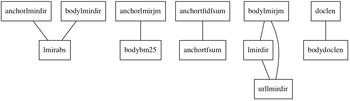
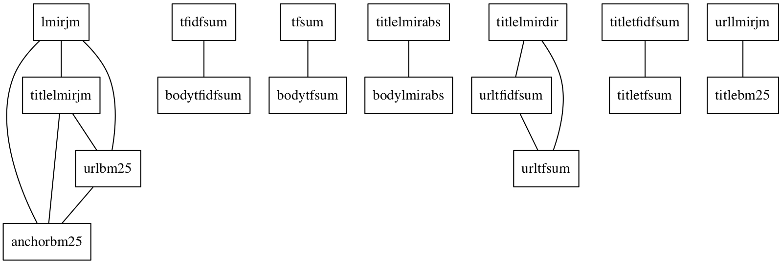
Figure 1: Highly collinear variables in LETOR. Each connected subgraph represents a subset of highly collinear variables. An edge was added when the Pearson correlation coefficient was 0.90 or more.

We found high collinearity ($0.90+$) between some variables of both datasets. A variable can thus be kept for each cluster of collinear variables and the other variables can be ignored. The removal of highly collinear variables might be necessary, since the specific software tool used by a researcher to estimate the parameters of a structural equation model may process complete covariance matrices and not only the variables of the model. We removed the most specific features and kept the most general; for example, we kept term frequency within a document and removed term frequency within the document title. The criteria to ignore a variable depends on the ease of interpretation of the SEM results, since the results will not significantly change with the ignored variables. Table 4 summarizes what was ignored and what was kept.

Table 4: Highly collinear variables kept for or ignored from analysis.

Variable kept	Variables ignored
anchortfsum	anchortfidfsum
titlelmirdir	urltfidfsum, urltfsum
titletfsum	titletfidfsum
tfidfsum	bodytfidfsum
tfsum	bodytfsum
bodybm25	anchorlmirjm
lmirdir	bodylmirjm, urllmirdir
lmirjm	titlelmirjm, urlbm25, anchorbm25
bodylmirabs	titlelmirabs
lmirabs	anchorlmirdir, bodylmirdir
titlebm25	urllmirjm
doclen	bodydoclen

The outliers of a variable have been mapped to the mean value of the variable to reduce the overall variability. We also applied $\log(x+\min x+1)$ to all exogenous variables $x$ to reduce non-normality and variability of the distribution of manifest exogenous variables and to make data closer to normal distribution. It is a standard practice in Statistics. There are other transformations. Usually, a transformation improves how well a particular SEM fits the data.

Kurtosis (i.e. heavier/lighter tails and a higher/lower peak than normal) and skewness (i.e. asymmetry about normal mean) were reduced, yet not completely eliminated. However, “children” of LETOR was still very skewed and leptokurtic. QQ-plotting allowed us to see that the lack of normality was due to a very few large values while the others were null; this variable was then ignored. The other variables exhibit lack of normality at very high or very low values. The middle values have a good fit with normality.

The manifest variables of LETOR have well-scaled variances, since the scale is 8:1, which is acceptable. Were the scale greater than hundreds, the values of the variables exhibiting the smallest variance should be multiplied by a certain factor until the scale becomes small.

Another approach can be based on reimplementing publicly documented retrieval algorithms. The difference between these two approaches lies in the degree of control of the retrieval functions. When using public datasets and runs, the researcher investigates the retrieval functions designed and implemented by other researchers, thus counting on the available documentation. When reimplementing publicly documented retrieval algorithms, the researcher may make decisions about some steps of indexing and retrieval which may make the implemented retrieval functions slightly different from similar functions. In particular, the latter approach allows the researcher to investigate his own retrieval functions. The experiments that are reported in Section 4.2 implemented the approach based on the reuse and combination of public datasets. In particular, two publicly available runs submitted to the Text REtrieval Conference (TREC) website and a public learning-to-rank dataset were utilised. We reproduced the runs obtained by a retrieval system based on BM25 and those obtained by a retrieval system based on TFIDF using the TIPSTER test collection. In our experiments, the discs 4 and 5 of the TIPSTER collection and the query sets of TREC-6, TREC-7 and TREC-8 were utilised to perform the experiments.

4.2 Use of Runs and Learning To Rank Datasets

Some structural equation models that are investigated in this paper include endogenous variables based on precision. Because precision is needed, document ranking was necessary. To obtain document ranking, we utilised two runs submitted to the TREC website for the 2007 Million Query track described by Allan et al. [2007]. Two runs described by Hiemstra et al. [2007] and produced using a full-text index built by Lucene [McCandless et al., 2010] were reused in our experiments to generate the endogenous variables of some structural equation models of this paper. One run was based on the Vector Space Model (VSM) (UAmsT07MTeVS) and the other was based on the Language Model (LM) (UAmsT07MTeLM).

Learning To Rank datasets were joined to the runs; in particular, for each run, every query-document pair of a run was linked to the corresponding record of document and query features. Thus, we had one record of features for each run, query, and document that can be in turn linked to the endogenous manifest variables that can measure retrieval effectiveness; we utilised the ratio between the numeric value of qrel and document rank. Each record of a run was joined with the corresponding record of features; for example, each record of UAmsT07MTeVS that refers to query $t$ and document $d$ was joined with the record of LETOR that refers to $t$ and $d$. In this way, each record of a run was an extended description of a retrieved document. As for LETOR, we considered query 5440, for both runs, because the number of retrieved documents was relatively high (about 80 documents), thus allowing us to perform the experiments with a non-small sample.

The MSLR dataset was investigated through query 22636, which is related to a relatively high number of cases (809) and all the five relevance degrees were assigned to the cases. Two variables were highly collinear if the correlation was 0.975 or more [Kline, 2015]. Some methods are suggested in the literature, yet thresholds are empirically chosen. Something similar happens with p-values which are compared with standard threshold (e.g. 0.01 or 0.05). In the paper, the thresholds were chosen by visual inspection; the threshold was the minimum value that induces disconnected and complete subgraphs of manifest variables as depicted by Figs. 1 and 2. The clusters of highly collinear variables are depicted in Fig. 2. After ignoring the highly collinear variables, the variables involved during the analysis are reported in Table 3. To reduce lack of normality of the remaining variables, the transformation $\log(x+min(x)+1)$ was applied to all exogenous variables. Unlike LETOR, the ratio between the maximum variance and the minimum variance was very high (12/0.001) in MSLR. As the large distance between maximum variance and minimum variance would cause problems during parameter estimation, it was progressively reduced by doubling the variable with minimum variance until the ratio was not greater than 10. (see the algorithm of Fig. 3).

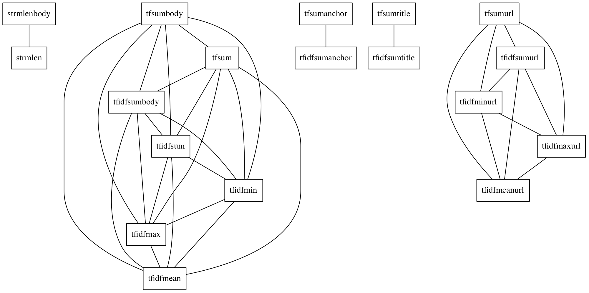
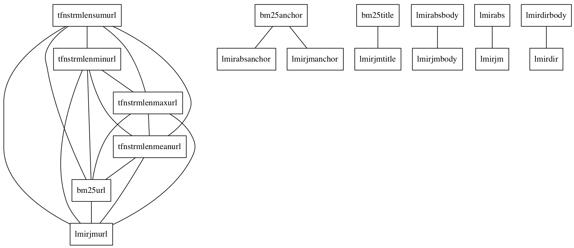
Figure 2: Highly collinear variables in MSLR for query 22636. Each connected subgraph represents a subset of highly collinear variables. An edge was added when the Pearson correlation coefficient was 0.975 or more.

	1	2	3	4	5	6	7	8	9	10	11	12	13	14	15
qtnbody	-1	0	0	0	0	0	1	0	0	0	0	0	0	1	0
qtnanchor	0	-1	-1	1	0	0	0	0	0	0	0	1	0	0	-1
qtntitle	-1	0	0	0	0	0	0	1	0	-1	0	0	-1	1	0
qtnurl	0	-1	1	0	-1	0	0	0	0	-1	0	0	-1	-1	1
qtn	-1	0	0	0	0	0	1	0	0	0	-1	-1	-1	0	0
strmlenanchor	0	-1	-1	0	0	0	0	0	0	0	-1	-1	0	0	0
strmlentitle	-1	0	0	-1	0	-1	-1	-1	-1	1	-1	0	0	0	1
strmlenurl	0	-1	0	-1	1	1	0	1	1	1	-1	0	-1	0	0
strmlen	-1	0	0	-1	0	-1	0	0	0	0	0	0	0	0	0
tfnstrmlensumbody	-1	0	0	1	0	1	0	0	1	1	1	0	1	0	1
tfnstrmlensumanchor	0	-1	-1	1	0	0	0	0	0	0	0	1	0	0	0
tfnstrmlensumtitle	-1	0	0	0	1	1	-1	1	1	-1	1	0	0	0	0
tfnstrmlensum	-1	0	1	1	0	1	0	-1	0	1	0	0	1	-1	0
tfidfsumanchor	0	-1	-1	1	0	0	0	0	0	0	0	0	0	0	0
tfidfsumtitle	-1	0	0	0	0	0	-1	0	0	0	0	0	0	0	0
tfidfsumurl	0	-1	1	0	-1	0	0	0	0	-1	0	0	0	0	0
tfidfsum	-1	0	0	0	0	-1	0	-1	0	1	0	0	0	0	0
bm25body	-1	0	0	0	0	0	1	0	0	0	0	0	0	1	0
bm25anchor	0	-1	-1	1	0	0	0	0	0	0	0	1	0	0	0
bm25title	-1	0	0	0	0	0	-1	1	0	-1	0	0	0	0	0
bm25url	0	-1	1	0	-1	0	0	0	0	-1	0	0	0	0	1
bm25	-1	0	0	0	0	0	1	0	0	0	-1	0	0	0	0
lmirabsbody	-1	0	0	0	0	0	1	0	0	0	0	0	0	0	0
lmirabstitle	-1	0	0	0	1	0	-1	1	0	-1	0	0	0	0	0
lmirabsurl	0	-1	1	0	-1	0	0	0	-1	-1	1	0	0	0	0
lmirabs	-1	0	1	1	0	1	1	0	0	0	-1	0	0	0	0
lmirdiranchor	0	-1	-1	0	-1	0	0	1	0	0	1	-1	1	1	1
lmirdirtitle	-1	0	0	0	0	0	-1	-1	-1	1	-1	0	1	-1	0
lmirdirurl	0	-1	1	-1	-1	0	0	1	-1	1	0	-1	1	1	-1
lmirdir	-1	0	0	0	0	-1	0	-1	0	1	0	0	0	0	0
slashes	0	-1	0	-1	1	1	0	0	1	0	-1	0	0	0	0
urllen	0	-1	0	-1	1	0	0	1	1	1	-1	0	-1	1	0
inlink	0	-1	-1	0	1	1	0	-1	0	-1	1	-1	0	-1	-1
outlink	0	-1	0	-1	0	-1	0	-1	1	1	1	0	0	-1	0
pagerank	0	0	-1	-1	-1	1	-1	-1	-1	0	1	0	-1	1	0
siterank	0	-1	-1	-1	0	1	0	-1	0	1	1	1	-1	0	0
quality	1	0	0	1	0	0	-1	0	0	1	1	0	-1	1	0
badness	0	0	1	1	0	-1	-1	-1	0	1	0	-1	-1	0	-1
query_url_clickcount	0	0	0	0	-1	0	-1	-1	1	-1	-1	0	1	1	0
url_clickcount	0	1	-1	-1	-1	0	0	1	1	1	-1	-1	-1	-1	0
url_dwell_time	0	1	-1	0	-1	0	0	1	0	0	-1	-1	-1	-1	0

Table 5: The first 16 principal components of the MSLR rescaled variables for query 22636

0:  Dataset of $k$ manifest variables, $X_{1},\dots,X_{k}$

  $\text{illscaled}\leftarrow\text{TRUE}$

  while illscaled do

     $i_{\max}\leftarrow\arg_{i=1,\dots,k}\max{\text{var}(X_{i})}$

     $i_{\min}\leftarrow\arg_{i=1,\dots,k}\min{\text{var}(X_{i})}$

     if $\text{var}(X_{i_{\max}})/\text{var}(X_{i_{\min}})\leq 10$ then

        $\text{illscaled}\leftarrow\text{FALSE}$

     else

        $X_{i_{\min}}\leftarrow 2X_{i_{\min}}$

     end if

  end while

Figure 3: The algorithm used to rescale the variables until the variances were no longer ill-scaled.

In the following sections, some analysis of experimental retrieval results have been illustrated.

4.3 Testing What Affect Effectiveness

Consider the manifest variables of UAmsT07MTeVS and UAmsT07MTeLM after applying the logarithmic transformation to reduce non-normality.

As mentioned above, the endogenous variable was the ratio between the numeric value of qrel and document rank. In order to reduce the variability, a log-transformation was applied to this ratio too. As the numeric value of qrel may be zero and a log-transformation cannot be applied to zero, the actual transformation was $Y=\log(\mbox{qrel}+1)/(\mbox{rank}+1)$ where qrel is the numeric value of qrel. The argument of the logarithmic function is positive when the document at the rank of the denominator is relevant and decreases when rank increases. It is a precision measure at the level of document since it is the contribution of a document to precision. Instead, P@$r$ is a measure of precision at the level of document list since it is the precision while the sublist of the top $r$ documents is scanned. The $Y$ defined above is preferable to P@$r$ because the analysis performed on UAmsT07MTeVS and UAmsT07MTeLM was at the level of document – the LETOR records were indeed joined to documents and not to lists.

After preparing the data, we looked for the best path model fitting the exogenous variables to the endogenous variable that measure retrieval effectiveness. To this end, a process of experimenting with various path models was performed until a good fit was found. In the experiments of this paper, the path model for UAmsT07MTeVS was $Y\leftarrow\log(\mbox{bodybm25}+1)+\log(\mbox{titlebm25}+1)+\log(\mbox{anchortfsum}+1)$ and that for UAmsT07MTeLM was $Y\leftarrow\log(\mbox{bodybm25}+1)+\log(\mbox{lmirjm}+1)+\log(\mbox{tfsum}+1)$. Two structural equation models have been tested in the experiments:

$$Y = B_{\mbox{\scriptsize bodybm25}}\log(\mbox{bodybm25}+1)+$$

$$B_{\mbox{\scriptsize titlebm25}}\log(\mbox{titlebm25}+1)+$$

$$B_{\mbox{\scriptsize anchortfsum}}\log(\mbox{anchortfsum}+1)$$

for UAmsT07MTeVS and

$$Y = B_{\mbox{\scriptsize bodybm25}}\log(\mbox{bodybm25}+1)+$$

$$B_{\mbox{\scriptsize lmirjm}}\log(\mbox{lmirjm}+1)+$$

$$B_{\mbox{\scriptsize tfsum}}\log(\mbox{tfsum}+1)$$

for UAmsT07MTeLM. An exogenous variable was significant when its regression coefficient was statistically significant ($\mbox{p-value}\approx 0$); the variables of the two structural equation models have significant regression coefficients, in particular,

$$B_{\mbox{\scriptsize bodybm25}}=6.55$$

$$B_{\mbox{\scriptsize titlebm25}}=5.10$$

$$B_{\mbox{\scriptsize anchortfsum}}=-1.67$$

for UAmsT07MTeVS and

$$B_{\mbox{\scriptsize tfsum}}=1.89$$

$$B_{\mbox{\scriptsize lmirjm}}=9.10$$

$$B_{\mbox{\scriptsize bodybm25}}=1.45$$

for UAmsT07MTeLM. The beta coefficients are

$$\beta_{\mbox{\scriptsize bodybm25}}=0.44$$

$$\beta_{\mbox{\scriptsize titlebm25}}=0.64$$

$$\beta_{\mbox{\scriptsize anchortfsum}}=-0.10$$

for UAmsT07MTeVS and

$$\beta_{\mbox{\scriptsize tfsum}}=0.15$$

$$\beta_{\mbox{\scriptsize lmirjm}}=0.87$$

$$\beta_{\mbox{\scriptsize bodybm25}}=0.10$$

for UAmsT07MTeLM, thus confirming the role played by BM25 – early introduced by Robertson and Walker [1994] – and LM – proposed by Ponte and Croft [1998] – for these two runs. Using the proportion of variance explained by all manifest variables with direct effects on the endogenous variable, we have a measure of goodness-of-fit $R^{2}$. The $R^{2}$’s values of the two models were $0.85$ and $0.90$ respectively for UAmsT07MTeLM and UAmsT07MTeVS, thus suggesting a good fit of the endogenous variable.

Finding the best path models was not a straightforward process. Indeed, given the endogenous variable, a path model is defined on the basis of a subset of exogenous variables, therefore, the best path model was the subset of exogenous variables that best fit the endogenous variable. Moreover, the process to find the best fit is manual and based on the researcher’s knowledge of the application domain. The difficulty of finding the best fit is hampered by the potential complete enumeration all the possible subsets, whose exponential number is $2$ to the power of the number of exogenous variables, the latter requiring an infeasible amount of work even for not large numbers. To cope with this exponential order, the semantics of the exogenous variables and the description of the retrieval algorithm utilised to produce a run helped select the most appropriate variables; for example, pagerank, which was computed by the PageRank algorithm introduced by Brin and Page [1998], is unlikely to correlate with effectiveness when UAmsT07MTeVS is considered, whereas tfsum would be more appropriate. Although the researcher’s knowledge of the application domain seems necessary to limit the space of subsets of exogenous variables, it is still likely that some subsets might be missed, thus making the selected structural equation models less than optimal.

As for UAmsT07MTeLM, the type of smoothing plays a crucial role because the effectiveness of the exogenous variable explaining the endogenous variable changes with smoothing technique. Indeed, $R^{2}$ significantly decreases if lmirjm is replaced with lmirdir or lmirabs, the latter being an outcome explained by the negative correlation between lmirjm and lmirdir ($\mbox{p-value}<0.05$) and that between lmirjm and lmirabs ($\mbox{p-value}<0.01$).

In contrast, the importance of bodybm25, which is the backbone of the probabilistic models, for the VSM-based run is worth noting especially if it is compared with the importance of the variables significantly related to the VSM such as anchortfsum. However, the important role played by bm25 should not come as a complete surprise. The sum of TFIDF weights (tfidfsum) provided by LETOR has been computed using a mathematical formulation different from the formulation implemented by modern VSM retrieval systems such as Lucene, which was used in the experiments reported by Hiemstra et al. [2007]. Indeed, the Lucene formulation is more similar to BM25 than to the LETOR’s tfidfsum, thus explaining why bodybm25 explains retrieval effectiveness in the VSM-based run. The small statistical correlation between bodytfidfsum and bodybm25 has further confirmed that their mathematical formulations were different. The main reason for this discrepancy was due to doclen, which is the most correlated variable with both bodytfidfsum and bodybm25 (both p-values were not greater than 0.01): the correlation between doclen and bodytfidfsum was positive, whereas that between doclen and bodybm25 was negative.

The role played by BM25 in the VSM-based run mentioned above might be considered an example of what SEM can suggest when applied to investigate experimental results. Some variables that are absent from a ranking function may have a role in a revised ranking function because they are significantly related to retrieval effectiveness in so far as its beta coefficient suggests. The revised ranking function may include the new variable using some mathematical or algorithmic rule decided by the researcher hoping that the new variable can boost the ranks of retrieved relevant documents or the retrieval of additional relevant documents.

The goodness-of-fit changes when the LM scores utilised as exogenous variables are those calculated from document parts other than the complete document; for example, if lmirjm is replaced with bodylmirjm, $R^{2}$ decreases. Similarly, the effectiveness of BM25 in explaining the endogenous variable of UAmsT07MTeVS depends on the document part from which the estimation data are extracted; for example, when bodybm25 is replaced with bm25 the goodness-of-fit decreases considerably, thus suggesting that the distribution of the terms significantly changes when it is estimated from different document parts.

Structural equation modeling depends on query and on run; indeed, testing the models found for query 5440 and applied to UAmsT07MTeLM and UAmsT07MTeVS for another query (e.g. 2297) gave unsatisfactory results as shown by the significant decrement of $R^{2}$. This outcome and the dependencies of the document parts from which estimation is performed are both an issue and a strength of the SEM-based approach to diagnose IR evaluation. On the one hand, it is an issue because a structural equation model has to be found for each retrieval algorithm (i.e. run) and for each query, and finding such a model requires an intellectual effort of the researcher who has to apply his expertise in the application domain being investigated by means of SEM for each run and query. On the other hand, the adaptation of the structural equation model to both run and query can provide an in-depth description of the retrieval system’s performance for each query and can make the failure analysis at the level of query possible and effective. Such a dependency calls from fully or semi-automatic methods for generating and testing structural equation models that can support the IR researcher in analysing the successes and the failures of a retrieval system.

4.4 Testing Latent Variables Behind Manifest Variables

In IR, researchers often assume the presence of latent variables such as relevance, authoritativeness (introduced by Brin and Page [1998] and Kleinberg [1999]) and eliteness (introduced by Harter [1975a]) behind the observed variables such as term frequencies and qrels. For example, the fact that relevance cannot be reduced to aboutness and that further dimensions of relevance such as document authoritativeness and quality should be considered in a retrieval function is by now well accepted. Another example is the metaphor of the LM approach introduced by Ponte and Croft [1998]. It assumes that both the authors of a document and the users who assess the document as relevant write the document and queries, respectively, that are about the same query, thus establishing a relationship between relevance and aboutness.

Another case of structural equation model including latent variables describes the relationship between eliteness, relevance and term frequency hypothesized by Robertson and Zaragoza [2009] in the context of BM25 and stemmed from the intuition given by Harter [1975a] 1975a, 1975b that term eliteness can be related to relevance. According to the relationship between eliteness, relevance and term frequency, for any document-term pair, eliteness is a latent property such that if the term is elite, then the document is about the concept represented by the term. Eliteness cannot be observed directly because it a latent variable. Manifest variables such as qrels and term frequency are indirect manifestations of eliteness. Specifically, this relationship can be described as follows: (1) eliteness is a property of a document-term pair such that if the term is elite in the document, in a sense the document is about the concept denoted by the term; (2) aboutness is a property of a document-query pair such that if the document is about a concept denoted by a query term, the document is relevant to the information need described by the query. These relations would be enough to explain the association between term frequency and relevance to the query. The relationship between eliteness, aboutness and relevance can be viewed as an example of what has been illustrated in this paper, that is, how relationships of this kind can be formalised as linear equations relating exogenous or endogenous variables and manifest or latent variables using a methodology based on a relatively simple mathematical model.

Using SEM, it is possible to formulate the eliteness model using the following structural equation model:

$$\mbox{qrel}\rightarrow\mbox{eliteness}\rightarrow\log\mbox{tfsum}$$ (2)

where eliteness is a latent variable whereas tfsum and qrel are manifest variables. This model postulates that relevance “causes” eliteness that in turn “causes” tfsum. Using UAmsT07MTeVS for query 5440, the relationship between qrel and eliteness is not significant ($\mbox{p-value}=0.637$), whereas that between tfsum and eliteness is significant ($\mbox{p-value}\approx 0$). This structural equation model and the regression coefficients thereof should not be rejected according to the chi-square test ($\mbox{p-value}=0.637$). The empirical numbers for CFI and RMSEA are 1 and 0, respectively, because the number of observations equals the number of parameters. In the example, the parameters are the direct effects (arrows) on endogenous variables (eliteness, log(tfsum)) as well as the variances of the exogenous variable (qrel). The observations of the model are the variances and covariances of the manifest variables (qrel, log(tfsum)).

The suggestion that the structural equation model (2) should not be rejected means that the hypothesis that eliteness is not significantly caused by relevance should not be rejected, thus not confirming the hypothesis made by Robertson and Zaragoza [2009]. However, the following slightly different structural equation model

$$\mbox{qrel}\rightarrow\mbox{eliteness}\rightarrow\log\mbox{bm25}$$ (3)

suggests that that hypothesis should be considered because the relationship between eliteness and qrel is significant.

Tests of the structural equation model (2) were replicated over all the queries in the LETOR data set to show that SEM can be applied to the level of runs as well. The documents retrieved by UAmsT07MTeLM were first joined with their features and then grouped by query. For each query, the average value of each feature and the NDCG value for that query were computed, thus obtaining a data set at the level of query. The fit of the structural equation model was extremely good. We found that tfsum can be determined by eliteness because the regression coefficient was about 0.35 and the p-value was about zero, but qrel does not determine eliteness because the regression coefficient was not significant. The p-value of the model was about 0.6, thus it cannot be rejected. Similar results were obtained by testing the structural equation model (3) or by replacing qrel with NDCG, which was introduced by Jarvëlin and Kekäläinen [2002].

Another example of the use of CFA in IR is the investigation of the coexistence of authoritativeness and aboutness as two distinct latent variables in the same document. A document can be viewed as authoritative when is able to be trusted as being accurate, true or reliable; other terms that are used to describe this document features are credibility or veracity; in contextual IR, authoritativeness can be viewed as a factor of document quality Melucci [2012] and can be measured by, for example, PageRank. The following model in which qrel can be a manifestation of both latent variables may model the coexistence of authoritativeness and aboutness as two distinct latent variables in the same document:

authoritativeness $$\rightarrow \mbox{pagerank}+\mbox{indegree}+$$ (5)

$$\mbox{urldepth}+\mbox{qrel}$$

aboutness $$\rightarrow \mbox{doclen}+\mbox{bm25}+\mbox{qrel}$$ (6)

authoritativeness $$\leftrightarrow$$ aboutness (7)

where the regression coefficients of (5) are

$$B_{\mbox{\scriptsize pagerank}} = 0.044$$

$$B_{\mbox{\scriptsize indegree}} = 0.006$$

$$B_{\mbox{\scriptsize urldepth}} = -0.043$$

$$B_{\mbox{\scriptsize qrel}} = 0.022$$

and the regression coefficients of (6) are

$$B_{\mbox{\scriptsize doclen}} = 0.137$$

$$B_{\mbox{\scriptsize bm25}} = -0.047$$

$$B_{\mbox{\scriptsize qrel}} = 0.396$$

These coefficients are statistically significant with $\mbox{p-value}<0.01$ except for $B_{\mbox{\scriptsize qrel}}$ of (5). The correlation between authoritativeness and aboutness is insignificant. This model passes the chi-square exact-fit test ($\mbox{p-value}=0.116$) as confirmed by $\mbox{\acs{CFI}}=0.934$. It also passes the approximate fit test since $\mbox{\acs{RMSEA}}=0.089$ ($\mbox{p-value}=0.212$).

Latent variables were investigated also using MSLR. Besides including many more variables than LETOR, MSLR also includes variables about the behaviour of the users who visited the pages described in the dataset and a couple of variables about the quality of the pages visited by the users. The variety of manifest variables of MSLR allowed us to make some hypotheses about the latent variables that may affect retrieval effectiveness. In particular, it was hypothesized that four latent variables, i.e. content, link, graph, page and user, may explain the manifest endogenous variable named “qrel” that encodes retrieval effectiveness (qrel ranges from 0 to 4). The latent variable “content” was about the informative content (i.e. keywords) of the pages that matched the query’s informative content. The latent variable “link” was about the informative content stored in the URLs and in the link anchors that matched the query’s informative content. The latent variable “graph” was about the graphical properties of the World Wide Web (WWW) node that corresponds to the page. The latent variable “user” was about the behaviour of the user who visited the page. The latent variable “page” was about the quality of the page. Thus, we have the following structural equation model:

qrel $$\leftarrow \mbox{content}+\mbox{link}+\mbox{graph}+\mbox{quality}+\mbox{user}$$

content $$\rightarrow \mbox{qtnbody}+\mbox{qtntitle}+\mbox{qtn}+\mbox{strmlentitle}+$$

$$\mbox{strmlen}+\mbox{tfnstrmlensumbody}+\mbox{tfnstrmlensumtitle}$$

$$+\mbox{tfnstrmlensum}+\mbox{tfidfsumtitle}+\mbox{tfidfsum}+$$

$$\mbox{bm25title}+\mbox{bm25}+\mbox{lmirabsbody}+$$

$$\mbox{lmirabstitle}+\mbox{lmirabs}+\mbox{lmirdirtitle}$$

graph $$\rightarrow \mbox{pagerank}+\mbox{inlink}+\mbox{outlink}+\mbox{siterank}$$

link $$\rightarrow \mbox{qtnurl}+\mbox{strmlenanchor}+\mbox{strmlenurl}$$

$$+\mbox{tfnstrmlensumanchor}+\mbox{tfidfsumanchor}+\mbox{tfidfsumurl}$$

$$+\mbox{bm25anchor}+\mbox{bm25url}+\mbox{lmirabsurl}+$$

$$\mbox{lmirdiranchor}+\mbox{lmirdirurl}$$

page $$\rightarrow \mbox{quality}+\mbox{badness}$$

user $$\rightarrow \mbox{query\_url\_clickcount}+\mbox{url\_clickcount}$$

The goodness-of-fit analysis of the structural equation model above came to contradictory indexes. CFI and TLI were relatively high (0.921 and 0.913, respectively) yet RMSEA was not very small (0.114) and its p-value was approximately zero, thus suggesting that the close fit hypothesis should be rejected. Besides, only the latent variable “user” was a significant latent variable explaining relevance (i.e. qrel). The regression coefficient was indeed 0.230 (p-value was approximately zero), thus suggesting that the number of clicks was a good predictor of relevance and that content, graph, link and page were little significant in explaining relevance. As for the relationships between latent variables and manifest variables, the variables based on “qtn”, TFIDF and LM were the most significant in explaining content, inlink was the most significant in explaining graph, the variables based on “anchor” in explaining url, quality in explaining page, and url_clickcount was the most significant manifest variable in explaining user.

SEM cannot suggest true conceptual relationships nor can it tell whether a variable can be the cause of another variable. As regards the eliteness-frequency-relevance relationship, in particular, SEM cannot suggest the true structural equation model; it can only tell whether the observed data fit the given structural equation model. It follows that a structural equation model might not be the only model that fit the observed data and that an alternative model may fit the data as well. For example, the following structural equation model

$$\mbox{qrel}\rightarrow\mbox{eliteness}\rightarrow\log\mbox{bm25}+\mbox{doclen}$$ (8)

is another good fit of the observed data. The problem with the (8) is that an IR researcher would perceive eliteness as little likely related to doclen although the regression coefficient is significantly different from zero and the approximate fit indexes suggest that the model is a good fit. In general, adding variables does not always decrease the fit, but it makes a model less readable than another model that includes fewer variables.

Latent variable names cannot be provided by SEM which leaves a great deal of freedom to the researcher who might, for example, replace “eliteness” with “aboutness” and obtain the same good approximate fit of the same structural equation model, which first explains aboutness by relevance and then explains bm25 and doclen by aboutness. The naming just mentioned is an example of naming fallacy. The name of a latent variable cannot be considered a sufficient condition that the latent variable is correct. However, latent variables have to be named to make them explicit to other researchers and in general to readers. In other domains, the issue is the same; for example, designers of database conceptual schemas name entities and relationships and report on their meanings by means of glossaries; moreover, data miners test clustering algorithms that yield clusters that should be named and described to convey the nature of the cluster points. The semantics of a structural equation model does not only depend on names, but it is also given by the complex of variables and associations. Besides, the seeming limitation can be surpassed by explicitly reporting the meaning of the names used in a structural equation model.

Another issue of SEM is that a latent variable might not correspond to an entity conceived by everyone in only one way; for example, eliteness might be conceived as a small subset of terms by a researcher, whereas it might be conceived as a more complex entity by another researcher. Since latent variable names are usually nouns, they suffer from the usual natural language drawbacks; for example, a latent variable name may be a synonym of another name or may be polysemous and carry more than one meaning at the same time.

Authoritativeness and aboutness are unrelated as shown by (7). This outcome confirms the early literature on the use of link analysis in IR in that authoritativeness and aboutness should be considered as distinct dimensions of relevance, capturing different user’s information needs; some users may require authoritative documents which might be little relevant while other users may require relevant documents yet little authoritative. The lack of relationship between authoritativeness and aboutness can also be observed by the lack of significance of the regression coefficient of qrel in (6) as opposed to the significance of qrel in (5), thus suggesting that qrel can be a signal of aboutness and not of authoritativeness.

Indegree and pagerank are both significant manifestations of authoritativeness. One reason for this simultaneous, significant manifestation may be due to the relationship between pagerank and indegree. Although it is a more complex algorithm than simply counting in-links, PageRank and indegree are strongly correlated (Pearson’s product-moment correlation comes out to be $0.832$ with $\mbox{p-value}\approx 0$). To check the hypothesis that pagerank might be removed from (5), the fit of the structural equation model introduced above has been recalculated without pagerank, thus obtaining very similar results: exact fit test passed with $\mbox{p-value}=0.570$; approximate fit test passed with $\mbox{p-value}=0.662$; $\mbox{\acs{CFI}}=1$.

The structural equation model that relates relevance degree (i.e. qrel) to five latent variables (i.e. content, user, link, graph, and quality) was only partially satisfactory, at least as far as query 22636 of MSLR is concerned. The unsatisfactory fit of this structural equation model suggests that the latent variables causing qrel might be less straightforward than those encoded by content, user, link, graph, and page, the latter often being utilised to model contextual search according to Melucci [2012], O’Brien and Toms [2013] and Park [2014]. For example, a manifest variable should be related to more than one latent variable in an improved structural equation model; however, the addition of relationships between variables might make a model unidentifiable.

To overcome the limitations on the generality of the results caused by the utilisation of one query, automated tools that perform such an analysis for many queries and datasets should be designed and implemented. As regards the goodness-of-fit of the structural equation model, although the approximate close indexes (CFI and TLI) were relatively high, other statistics suggested that better models should be found (for example RMSEA was not very small). Unfortunately, SEM cannot straightforwardly suggest the correct and best model unless the researcher helps to find such a model by using his knowledge of the application domain, yet some help can be given by stepwise regression.

4.5 Effect of Query Terms

In this section, the impact of the query term weights of Lucene’s implementation of the VSM-based retrieval function and that of the BM25-based retrieval function will be investigated. The VSM-based retrieval function is a modification of the classical VSM retrieval function and was applied for each query $Q$ and document $D$ as follows:

$$\sum_{t\in Q}\mbox{dtw}_{t,D}\mbox{qtw}_{t,Q}\mbox{coord}_{Q,D}\mbox{boost}_{t}$$ (9)

where

$$\mbox{dtw}_{t,D} = \frac{\mbox{tfidf}_{t,D}}{\mbox{length}_{D}}$$

$$\mbox{qtw}_{t,Q} = \frac{\mbox{tfidf}_{t,Q}}{\mbox{length}_{Q}}$$

$$\mbox{coord}_{Q,D} = \frac{|D\cap Q|}{|Q|}$$

$$\mbox{boost}_{t} = 1$$

On the other hand, the BM25-based run was obtained by the following retrieval function

$$\sum_{t\in Q}\mbox{idf}_{t}\mbox{sat}_{t,D}$$ (10)

where

$$\mbox{idf}_{t,D} = \log\frac{N-\mbox{df}_{t}+0.5}{\mbox{df}_{t}+0.5}$$

$$\mbox{sat}_{t} = \frac{\mbox{tf}_{t,D}}{K+\mbox{tf}_{t,D}}$$

$$K = k_{1}\left(1-b+b\frac{\mbox{doclen}}{\mbox{avdoclen}}\right)$$

For each query, two lists of documents were created – one list for each retrieval function. Each retrieved document has been associated to the assessment of relevance to the query and was joined to the components of the weight function of each query term. In particular, each document retrieved by the VSM-based retrieval function was joined to $\mbox{dtw}_{t,D},\mbox{qtw}_{t,Q},\mbox{coord}_{Q,D},\mbox{boost}_{t}$ for each query term $t$, and each document retrieved by the BM25-based retrieval function was joined to $\mbox{idf}_{t}\mbox{sat}_{t,D}$ for each query term $t$. Moreover, P@$r$ was computed for each document retrieved at rank $r$.

The following structural equation model was estimated as for the BM25-based run and query 305 (“Most Dangerous Vehicles: Which are the most crashworthy, and least crashworthy, passenger vehicles?”):

prec $$\leftarrow \mbox{bm25}_{\mbox{\scriptsize crashworthy}}+\mbox{bm25}_{\mbox{\scriptsize dangerous}}+$$

$$\mbox{bm25}_{\mbox{\scriptsize passenger}}+\mbox{bm25}_{\mbox{\scriptsize vehicles}}$$

The regression coefficients are as follows :

$$B_{\mbox{\scriptsize bm25,dangerous}} = 0.016$$

$$B_{\mbox{\scriptsize bm25,passenger}} = 0.023$$

$$B_{\mbox{\scriptsize bm25,vehicles}} = 0.017$$

As the p-values were approximately zero, the regression coefficients were significant; however, the fit was rather bad because of the low number of exogenous variables. Although the regression coefficients can be an interesting measure of the variation of prec, the beta coefficients were of greater interest because they provide a measure of the importance of each variable controlling the other variables. In particular, the beta coefficients were:

$$\beta_{\mbox{\scriptsize bm25,dangerous}} = 0.229$$

$$\beta_{\mbox{\scriptsize bm25,passenger}} = 0.397$$

$$\beta_{\mbox{\scriptsize bm25,vehicles}} = 0.342$$

The beta coefficients are larger than the corresponding regression coefficients because of the negative correlations between some pairs of BM25 weights. To investigate this model further, the following structural equation model that replaces the BM25 weights with their components (i.e. idf and sat) was estimated:

prec $$\leftarrow \mbox{idf}_{\mbox{\scriptsize dangerous}}+\mbox{sat}_{\mbox{\scriptsize dangerous}}+\mbox{idf}_{\mbox{\scriptsize passenger}}+$$

$$\mbox{sat}_{\mbox{\scriptsize passenger}}+\mbox{idf}_{\mbox{\scriptsize vehicles}}+\mbox{sat}_{\mbox{\scriptsize vehicles}}$$

The regression coefficients are as follows:

$$B_{\mbox{\scriptsize idf,dangerous}} = 0.002$$

$$B_{\mbox{\scriptsize idf,passenger}} = 0.023$$

$$B_{\mbox{\scriptsize idf,vehicles}} = 0.018$$

$$B_{\mbox{\scriptsize sat,dangerous}} = 0.047$$

$$B_{\mbox{\scriptsize sat,passenger}} = 0.102$$

$$B_{\mbox{\scriptsize sat,vehicles}} = 0.082$$

Except for $B_{\mbox{\scriptsize idf,dangerous}}$, these coefficients are significant. The corresponding beta coefficients are as follows:

$$\beta_{\mbox{\scriptsize idf,dangerous}} = -0.035$$

$$\beta_{\mbox{\scriptsize idf,passenger}} = -0.323$$

$$\beta_{\mbox{\scriptsize idf,vehicles}} = -0.340$$

$$\beta_{\mbox{\scriptsize sat,dangerous}} = 0.301$$

$$\beta_{\mbox{\scriptsize sat,passenger}} = 0.813$$

$$\beta_{\mbox{\scriptsize sat,vehicles}} = 0.857$$

The following structural equation model was estimated as for the VSM-based run:

prec $$\leftarrow \mbox{dtw}_{\mbox{\scriptsize crashworthy}}+\mbox{dtw}_{\mbox{\scriptsize dangerous}}+\mbox{dtw}_{\mbox{\scriptsize passenger}}+\mbox{dtw}_{\mbox{\scriptsize vehicles}}+$$

$$\mbox{qtw}_{\mbox{\scriptsize crashworthy}}+\mbox{qtw}_{\mbox{\scriptsize dangerous}}+\mbox{qtw}_{\mbox{\scriptsize passenger}}+\mbox{qtw}_{\mbox{\scriptsize vehicles}}$$

The regression coefficients are as follows and all were significant:

$$B_{\mbox{\scriptsize dtw,dangerous}} = 0.064$$

$$B_{\mbox{\scriptsize dtw,passenger}} = 0.095$$

$$B_{\mbox{\scriptsize dtw,vehicles}} = 0.078$$

$$B_{\mbox{\scriptsize qtw,dangerous}} = 0.088$$

$$B_{\mbox{\scriptsize qtw,passenger}} = 0.042$$

$$B_{\mbox{\scriptsize qtw,vehicles}} = 0.074$$

The beta coefficients were as follows:

$$\beta_{\mbox{\scriptsize dtw,dangerous}} = 0.341$$

$$\beta_{\mbox{\scriptsize dtw,passenger}} = 0.929$$

$$\beta_{\mbox{\scriptsize dtw,vehicles}} = 0.635$$

$$\beta_{\mbox{\scriptsize qtw,dangerous}} = 0.412$$

$$\beta_{\mbox{\scriptsize qtw,passenger}} = 0.205$$

$$\beta_{\mbox{\scriptsize qtw,vehicles}} = 0.331$$

The badness of fit of the structural equation models above depends on the low number of exogenous variables; the fit was very good when all the weight components were added to the model for each query term. A good fit may be useful for prediction purposes; however, it may be misleading when the role played by the BM25-based query term weights is of interest. It might be misleading because, if all the weight components were added to the model for each query term, the beta coefficients of the saturation weights would have the opposite sign of the BM25-based query term weights. The difference in sign between the beta coefficients of saturation and those of BM25 is counter-intuitive since both saturation and BM25 should be positively correlated to prec. However, the difference in sign is caused by the strong correlations between the weight components that make the beta coefficients negative. The high collinearity could be acceptable when the variables are due to natural processes such as the collinearity between height and weight. In the event, they are not caused by natural processes; on the contrary, they are caused by the mathematical formulation of the function which make BM25 functionally dependent on saturation and IDF. It follows that the exogenous variables of the weight components (e.g. IDF) should be ignored and not added to the structural equation model together with BM25 in the analysis.

The negative correlation between BM25 weights can be quite surprising since it is expected that all the query terms participate in increasing P@$r$. Instead, the results of the analysis suggest that when one query term contributes to retrieval effectiveness, another query term is detrimental – for query 305 and the BM25-based retrieval function at least. The beta coefficients of the four query terms above indicate the most important query terms as regards P@$r$ when document ranking is performed by the BM25-based retrieval function. When the retrieval functions are compared, the regression coefficients have to be used.

5 Conclusions and Future Directions

The crucial point of the use of SEM in data analytics is the definition of the structural equation models that describe the observed data at their best. It would be desirable to always find the best structural equation model, that is the model that fit the data very well on the basis of statistically significant parameters and of a reasonable narrative – from the researcher’s perspective at least. However, the best model cannot always be found, since two or more models may fit the observed data well or no fitting model may be found at all. Another weakness is the need to define structural equation models (e.g. path models) starting from many manifest variables. Although the researcher’s judgment should always be considered, manually finding the best model requires a considerable intellectual effort and some automatic method – semi-automatic at least – would be desirable.

In the area of learning-to-rank, in particular, and in that of Machine Learning, in general, a number of procedures for selecting features and fitting functions have been developed Liu [2011]. Although these procedures should be considered with reference to the problem of defining and estimating structural equation models, the selection of the variables of a structural equation model is a more complex task than the definition of real functions of the scores and weights which are observed for documents and terms to the aims of learning to rank. Variable selection has to do with the description of the retrieval models such as the VSM, the language models and the probabilistic models; the question is how to represent a retrieval model in terms of variables, relationships and therefore in terms of a structural equation model.

Moreover, further research would be advisable to find methods that “translate” a structural equation model into rules of modification for a more effective retrieval model once the structural equation model has been found for the retrieval model. Indeed, the ultimate goal of the use of SEM in IR evaluation would be the transformation of a retrieval model into a new, more effective model. Such a transformation resembles what the approaches to learning-to-rank aim for, that is, a set of parameters of a real function mapping an independent multi-variate variable to a dependent univariate variable.

The potential of SEM is the capacity to combine latent variables with manifest variables. The ability of using latent variables that may be developed may lead to implementing some general hypotheses about IR (e.g. the role played by authoritativeness or search task) and their influence on retrieval effectiveness. This ability may have some desirable effects. On the one hand, it may facilitate the investigation of the processes of information seeking based on the quantitative analysis provided by SEM. On the other hand, it may help the researchers to explain the results gathered throughout the course of their experiments by using more effective statistical instruments than descriptive or inferential statistics.

One distinguishing feature of SEM is the graphical nature of a structural equation model; such a model can be communicated in spoken or written words because variables and causal relationships thereof may be viewed as concepts (e.g. nouns) and associations (e.g. verbs). As a result of the graphical nature of a structural equation model, SEM may become a new language helping the researchers in IR to find more powerful descriptions and explanations of theoretical models and experimental results than traditional statistics.

Despite the potential expressed since Wright’s pioneering work 1918, some misunderstandings are still limiting the potential of SEM Bollen and Pearl [2013]. First, it is often believed that correlation implies causation and that a significant regression coefficient may be considered a strong signal that a variable is the cause of another variable. Instead, SEM cannot discover causal relationships other than the relationships already encoded in the researcher’s structural equation model. Second, SEM is often viewed as nothing but a complicated regression and ANOVA technique. Causal networks rather, allow the researchers to utilise a language that is not part of standard statistics for expressing their application domains differently from the way provided by regression and ANOVA Pearl [2009, 2012].

References

- Afzal [2013] W. Afzal. Rethinking information privacy-security: Does it really matter? Proceedings of ASIST, 50(1):1–10, 2013.
- Allan et al. [2007] J. Allan, B. Carterette, and J. A. Aslam. Million query track 2007 overview. In Proceedings of TREC, 2007.
- Azzopardi and Vinay [2008] L. Azzopardi and V. Vinay. Retrievability: An evaluation measure for higher order information access tasks. In Proceedings of CIKM, pages 561–570, 2008.
- Bailey et al. [2015] P. Bailey, A. Moffat, F. Scholer, and P. Thomas. User variability and IR system evaluation. In Proceedings of SIGIR, pages 625–634, 2015.
- Bartholomew et al. [2008] D. Bartholomew, F. Steele, and I. Moustaki. Analysis of multivariate social science data. Statistics in the social and behavioral sciences series. CRC Press, 2008.
- Belkin et al. [1982a] N. J. Belkin, R. Oddy, and H. M. Brooks. ASK for information retrieval. Part 1: Background and theory. Journal of Documentation, 38(2):61–71, 1982a. ISSN 0022-0418.
- Belkin et al. [1982b] N. J. Belkin, R. Oddy, and H. M. Brooks. ASK for information retrieval. Part 2: Results of a design study. Journal of Documentation, 38(3):145–164, 1982b. ISSN 0022-0418.
- Bentler [1990] P. M. Bentler. Comparative fit indexes in structural models. Psychological Bulletin, 107:238–246, 1990.
- Bigot et al. [2011] A. Bigot, C. Chrisment, T. Dkaki, G. Hubert, and J. Mothe. Fusing different information retrieval systems according to query-topics: a study based on correlation in information retrieval systems and trec topics. Information Retrieval, 14(6):617–648, 2011.
- Bollen and Pearl [2013] K. A. Bollen and J. Pearl. Eight myths about causality and structural equation models. In S. L. Morgan, editor, Handbook of causal analysis for social research, pages 301–328. Springer, 2013.
- Brin and Page [1998] S. Brin and L. Page. The anatomy of a large-scale hypertextual web search engine. In Proceedings of WWW, Brisbane, Australia, 1998. http://www7.scu.edu.au/.
- Buckley [2009] C. Buckley. Why current IR engines fail. Information Retrieval, 12(6):652–665, 2009.
- Butman et al. [2013] O. Butman, A. Shtok, O. Kurland, and D. Carmel. Query-performance prediction using minimal relevance feedback. In Proceedings of ICTIR, pages 14–21, 2013.
- Carterette [2011] B. Carterette. System effectiveness, user models, and user utility: A conceptual framework for investigation. In Proceedings of SIGIR, pages 903–912, 2011.
- Carterette et al. [2011] B. Carterette, E. Kanoulas, and E. Yilmaz. Simulating simple user behavior for system effectiveness evaluation. In Proceedings of CIKM, pages 611–620, 2011.
- Carterette et al. [2012] B. Carterette, E. Kanoulas, and E. Yilmaz. Incorporating variability in user behavior into systems based evaluation. In Proceedings of CIKM, pages 135–144, 2012.
- Chan et al. [2005] H. Chan, H. Teo, and X. Zeng. An evaluation of novice end-user computing performance: Data modeling, query writing, and comprehension. Journal of the American Society for Information Science and Technology, 56(8):843–853, 2005.
- Chen and Chiu [2007] G. Chen and M. M. Chiu. Effects of previous messages’ evaluations, knowledge content, social cues and personal information on the current message during online discussion. In Proceedings of CSCL, pages 135–137, 2007.
- Cho et al. [2010] H. Cho, M. Chen, and S. Chung. Testing an integrative theoretical model of knowledge-sharing behavior in the context of wikipedia. Journal of the American Society for Information Science and Technology, 61(6):1198–1212, 2010.
- Crescenzi et al. [2016] A. Crescenzi, D. Kelly, and L. Azzopardi. Impacts of time constraints and system delays on user experience. In Proceedings of CHIIR, pages 141–150, 2016.
- Cronen-Townsend et al. [2002] S. Cronen-Townsend, Y. Zhou, and W. B. Croft. Predicting query performance. In Proceedings of SIGIR, pages 299–306, 2002.
- Cummins [2014] R. Cummins. Document score distribution models for query performance inference and prediction. ACM Transactions on Information Systems, 32(1):1–28, 2014.
- Deerwester et al. [1990] S. Deerwester, S. Dumais, G. Furnas, T. Landauer, and R. Harshman. Indexing by latent semantic analysis. Journal of the American Society for Information Science and Technology, 41(6):391–407, 1990.
- Fang and Zhai [2005] H. Fang and C. Zhai. An exploration of axiomatic approaches to information retrieval. In Proceedings of SIGIR, pages 480–487, 2005.
- Fang et al. [2004] H. Fang, T. Tao, and C. Zhai. A formal study of information retrieval heuristics. In Proceedings of SIGIR, pages 49–56, 2004.
- Fang et al. [2011] H. Fang, T. Tao, and C. Zhai. Diagnostic evaluation of information retrieval models. ACM Transactions on Information Systems, 29(2):7:1–7:42, 2011.
- Harman and Buckley [2009] D. Harman and C. Buckley. Overview of the reliable information access workshop. Information Retrieval, 12:615–641, 2009.
- Harter [1975a] S. Harter. A probabilistic approach to automatic keyword indexing: part 1: On the distribution of specialty words in a technical literature. Journal of the American Society for Information Science, 26(4):197–206, 1975a.
- Harter [1975b] S. Harter. A probabilistic approach to automatic keyword indexing: part 2: An algorithm for probabilistic indexing. Journal of the American Society for Information Science, 26(5):280–289, 1975b.
- Hauff et al. [2008] C. Hauff, V. Murdock, and R. Baeza-Yates. Improved query difficulty prediction for the web. In Proceedings of CIKM, pages 439–448, 2008.
- Hauff et al. [2010] C. Hauff, D. Kelly, and L. Azzopardi. A comparison of user and system query performance predictions. In Proceedings of CIKM, pages 979–988, 2010.
- Hiemstra et al. [2007] D. Hiemstra, J. Kamps, R. Kaptein, and R. Li. Parsimonious language models for a terabyte of text. In Proceedings of TREC, 2007.
- Ishita et al. [2017] E. Ishita, Y. Miyata, S. Ueda, and K. Kurata. A structural equation model of information retrieval skills. In Proceedings of the 2017 Conference on Conference Human Information Interaction and Retrieval, CHIIR ’17, pages 317–320, New York, NY, USA, 2017. ACM. ISBN 978-1-4503-4677-1. doi: 10.1145/3020165.3022142. URL http://doi.acm.org/10.1145/3020165.3022142.
- Jarvëlin and Kekäläinen [2002] K. Jarvëlin and J. Kekäläinen. Cumulated gain-based evaluation of IR techniques. ACM Transactions on Information Systems, 20(4):422–446, 2002.
- Kattenbeck and Elsweiler [2018] M. Kattenbeck and D. Elsweiler. Estimating models combining latent and measured variables: A tutorial on basics, applications and current developments in structural equation models and their estimation using pls path modeling. In Proceedings of the 2018 Conference on Human Information Interaction & Retrieval, CHIIR ’18, pages 375–377, New York, NY, USA, 2018. ACM. ISBN 978-1-4503-4925-3. doi: 10.1145/3176349.3176899. URL http://doi.acm.org/10.1145/3176349.3176899.
- Kendall [1938] M. Kendall. A new measure of rank correlation. Biometrika, 30(1/2):81–93, June 1938.
- Kher et al. [2009] H. Kher, M. A. Serva, S. Davidson, and E. Monk. Leveraging latent growth models to better understand mis theory: A primer. In Proceedings of SIGMIS CPR, pages 159–166, 2009.
- Kim et al. [2013] Y. Kim, A. Hassan, R. W. White, and Y.-M. Wang. Playing by the rules: Mining query associations to predict search performance. In Proceedings of WSDM, pages 133–142, 2013.
- Kipp and Joo [2010] M. E. I. Kipp and S. Joo. Application of structural equation modelling in exploring tag patterns: A pilot study. Proceedings of ASIST, 47(1):1–2, 2010.
- Kleinberg [1999] J. Kleinberg. Authorative sources in a hyperlinked environment. Journal of the ACM, 46(5):604–632, 1999.
- Kline [2015] R. B. Kline. Principles and Practice of Structural Equation Modeling. The Guilford Press, fourth edition, 2015.
- Kurland et al. [2012] O. Kurland, A. Shtok, S. Hummel, F. Raiber, D. Carmel, and O. Rom. Back to the roots: A probabilistic framework for query-performance prediction. In Proceedings of CIKM, pages 823–832, 2012.
- Kwon and Onwuegbuzie [2005] N. Kwon and A. J. Onwuegbuzie. Modeling the factors affecting individuals’ use of community networks: A theoretical explanation of community-based information and communication technology use. joasist, 56(14):1525–1543, 2005.
- Liu [2011] T.-Y. Liu. Learning to Rank for Information Retrieval. Springer, 2011.
- Lu and Zhu [2010] C.-T. Lu and D.-S. Zhu. The study on the determinants of the online consumers’ intention to return. In Proceedings of IEEE ACIS, pages 289–294, 2010.
- Macdonald et al. [2013] C. Macdonald, R. Santos, and I. Ounis. The whens and hows of learning to rank for web search. Information Retrieval, 16(5):584–628, 2013.
- Marchionini and Crane [1994] G. Marchionini and G. Crane. Evaluating hypermedia and learning: Methods and results from the Perseus project. ACM Transactions on Information Systems, 12(1):5–34, Jan. 1994.
- Marchionini and Shneiderman [1988] G. Marchionini and B. Shneiderman. Finding facts vsa. browsing knowledge in hypertext systems. IEEE Computer, 21(1):70–80, 1988.
- McCandless et al. [2010] M. McCandless, E. Hatcher, and O. Gospodnetić. Lucene in action. Manning, 2010.
- Melucci [2012] M. Melucci. Contextual Search: A Computational Framework. Foundations and Trends in Information Retrieval. Now Publishers, 2012.
- O’Brien and Toms [2013] H. L. O’Brien and E. G. Toms. Examining the generalizability of the user engagement scale (ues) in exploratory search. Information Processing and Management, 49(5):1092–1107, 2013.
- Ogilvie et al. [2009] P. Ogilvie, E. Voorhees, and J. Callan. On the number of terms used in automatic query expansion. Information Retrieval, 12(6):666–679, 2009.
- Park [2014] J.-H. Park. The effects of personalization on user continuance in social networking sites. Information Processing and Management, 50(3):462–475, 2014.
- Pearl [2009] J. Pearl. Causality. Cambridge University Press, 2009.
- Pearl [2012] J. Pearl. The causal foundations of structural equation modeling. In R. H. Hoyle, editor, Handbook of structural equation modeling, pages 68–91. Guilford Press, 2012.
- Ponte and Croft [1998] J. Ponte and W. Croft. A language modeling approach to information retrieval. In Proceedings of SIGIR, pages 275–281, 1998.
- Qin et al. [2010] T. Qin, T.-Y. Liu, J. Xu, and H. Li. Letor: A benchmark collection for research on learning to rank for information retrieval. Information Retrieval, 13(4):346–374, 2010.
- Raiber and Kurland [2014] F. Raiber and O. Kurland. Query-performance prediction: Setting the expectations straight. In Proceedings of SIGIR, pages 13–22, 2014.
- Robertson and Walker [1994] S. Robertson and S. Walker. Some simple effective approximations to the 2-Poisson model for probabilistic weighted retrieval. In Proceedings of SIGIR, pages 232–241, 1994.
- Robertson and Zaragoza [2009] S. Robertson and H. Zaragoza. The probabilistic relevance framework: BM25 and beyond. Foundations and Trends in Information Retrieval, 3(4):333–389, 2009.
- Sakai [2014] T. Sakai. Designing test collections for comparing many systems. In Proceedings of CIKM, pages 61–70, 2014.
- Salton [1979] G. Salton. Mathematics and information retrieval. Journal of Documentation, 35(1):1–29, 1979.
- Senapathi and Srinivasan [2014] M. Senapathi and A. Srinivasan. An empirical investigation of the factors affecting agile usage. In Proceedings of ICEAS, pages 1–10, 2014.
- Sin [2010] S.-C. J. Sin. Modeling individual-level information behavior: A person-in-environment (pie) framework. Proceedings of ASIST, 47(1):1–4, 2010.
- Spearman [1904] C. Spearman. The proof and measurement of association between two things. The American Journal of Psychology, 15(1):72–101, 1904.
- Tucker and Lewis [1973] L. R. Tucker and C. Lewis. A reliability coefficient for maximum likelihood factor analysis. Psychometrika, 38:1–10, 1973.
- Vakkari and Järvelin [2005] P. Vakkari and K. Järvelin. Explanation in information seeking and retrieval. In A. Spink and C. Cole, editors, New Directions in Cognitive Information Retrieval. Springer, 2005.
- Voorhees and Buckley [2002] E. Voorhees and C. Buckley. The effect of topic set size on retrieval experiment error. In Proceedings of SIGIR, pages 316–323, 2002.
- Wilkie and Azzopardi [2014] C. Wilkie and L. Azzopardi. A retrievability analysis: exploring the relationship between retrieval bias and retrieval performance. In Proceedings of CIKM, pages 81–90, 2014.
- Wright [1918] S. Wright. On the nature of size factor. Genetics, 3(367), 1918.
- Zhang et al. [2014] Y. Zhang, J. Zhang, M. Lease, and J. Gwizdka. Multidimensional relevance modeling via psychometrics and crowdsourcing. In Proceedings of SIGIR, pages 435–444, 2014.
- Zhang and Dang [2015] Y. G. Zhang and Y. M. Dang. Investigating essential factors on students’ perceived accomplishment and enjoyment and intention to learn in web development. Trans. Comput. Educ., 15(1):1–21, 2015.
- Zhao et al. [2008] Y. Zhao, F. Scholer, and Y. Tsegay. Effective pre-retrieval query performance prediction using similarity and variability evidence. In Proceedings of ECIR, pages 52–64, 2008.
- Zhou and Croft [2006] Y. Zhou and W. B. Croft. Ranking robustness: A novel framework to predict query performance. In Proceedings of CIKM, pages 567–574, 2006.