Colliding cells: when active segments behave as active particles

Abstract

Quantifying the outcomes of cells collisions is a crucial step in building the foundations of a kinetic theory of living matter. Here, we develop a mechanical theory of such collisions by first representing individual cells as extended objects with internal activity and then reducing this description to a model of size-less active particles characterized by their position and polarity. We show that, in the presence of an applied force, a cell can either be dragged along or self-propel against the force, depending on the polarity of the cell. The co-existence of these regimes offers a self-consistent mechanical explanation for cell re-polarization upon contact. We rationalize the experimentally observed collision scenarios within the extended and particle models and link the various outcomes with measurable biological parameters.

Interacting cells is an important example of active matter and the modeling of their collective behavior is one of the main challenges for non-equilibrium statistical mechanics Marchetti et al. (2013). Since the configuration of emerging active phases crucially depends on cell-to-cell collisions Camley and Rappel (2017); Hakim and Silberzan (2017), the rationalization of collision tests is a prerequisite for the development of an adequate kinetic theory of living matter Vicsek et al. (1995); Peshkov et al. (2014). Building reliable links between the collison outcomes and measurable biophysical parameters is also fundamental for the control of development, integrity and regeneration of living organisms Friedl and Gilmour (2009); Trepat and Fredberg (2011); Gov (2011); Trepat et al. (2009); Gov (2009); Kabla (2012); Tambe et al. (2011); Garcia et al. (2015); Löber et al. (2015); Zimmermann et al. (2016); Smeets et al. (2016).

Experiments show that head-on collision of two polarized cells can result in four possible outcomes Desai et al. (2013); Scarpa et al. (2013): velocity reversal, representing a quasi-elastic collision with symmetric re-polarization, two quasi-inelastic scenarios with the formation of a cell doublet that can be either motile (train) or static (still) and finally, a bypass regime, when cells advance over each other Kulawiak et al. (2016).

The reversal and pairing regimes are usually associated with the phenomenon of contact inhibition of locomotion (CIL) Stramer and Mayor (2017). While CIL is crucial for healthy animal physiology, being a critical driver of cell dispersion, tiling and collective motility within embryonic tissues, the loss of CIL is usually associated with pathological processes, including cancer Stramer and Mayor (2017). The physical conditions provoking the failure of CIL remain largely unknown.

Many important advances have been made in the modeling of individual cells migration Jülicher et al. (2007); Rubinstein et al. (2009); Shao et al. (2010); Ziebert et al. (2011); Giomi and DeSimone (2014); Tjhung et al. (2015). The extra-complexity of cell collision is due to the involvement of additional mechanisms including coordinated bonding and re-polarization. The biological control of these processes may be complex, for instance, re-polarization has been recently modeled in reaction-diffusion frameworks with the focus on Rho-GTPase Rappel and Edelstein-Keshet (2017). This and other bio-chemical regulators of force production inside the cytoskeleton have been already incorporated in computational models of cell collision Merchant et al. (2017); Kulawiak et al. (2016).

Motivated by the experimental observations that a crucial building block of CIL is mysoin contractility Davis et al. (2015), we take an alternative path and study the possibility of capturing the known outcomes of a collision within a purely mechanical model. We first represent cells as extended segments of active gel (AS) Recho et al. (2013); Callan-Jones and Voituriez (2013) and then reduce this model to obtain an equivalent active particle (AP) description. In contrast to some well known representations of size-less active agents Romanczuk et al. (2012), the derived particle model contains an internal variable describing cell polarity which can be affected by the applied force. We show that this reduced AP model is able to adequately reproduce the outcomes of collision tests predicted by the AS model covering the whole set of possibilities observed experimentally.

Being exposed to an external force, both models support two coexisting dynamic regimes: frictional, when the active object is dragged by the force, and anti-frictional, when it is dragging the force. The fact that the system can jump from one of these nonequilibrium steady states to the other through a hysteresis loop offers a self-consistent mechanical explanation for cell re-polarization upon contact. In this description, re-polarization emerges as a result of the spontaneous self-organization of the cytoskeleton rather than an outcome of chemical regulation. The most important prediction of the model is that all four known cell collision scenarios can be accessed by tuning a single nondimensional parameter describing cell contractility.

We begin by representing a self-propelling cell as an AS which allows us to focus on the dynamics of its cytoskeletal meshwork. We use non-dimensional variables and assume that the segment is limited by two time-dependent fronts $x_{r}(t)<x_{f}(t)$ and has a fixed length $\mathcal{L}=x_{f}-x_{r}$. In this simplified setting, both fronts are moving at the same velocity $V(t)=\dot{S}$ where $S(t)=(x_{f}+x_{r})/2$ is the center of the segment and the superimposed dot denotes the time derivative. We further assume that the organization of the molecular motors in the segment is governed by the dimensionless drift-diffusion equation

$$\dot{c}+\partial_{y}\left(cv\right)=\partial_{yy}c,$$ (1)

where $y\in[-\mathcal{L}/2,\mathcal{L}/2]$ is a spatial coordinate labeling material points of the moving segment, $c(y,t)$ represents the concentration of motors and $v(y,t)$ is the mechanical velocity of the cytoskeleton relative to the motion of the cell fronts. We supplement (1) with no-flux boundary conditions $\partial_{y}c|_{\pm\mathcal{L}/2}=0$ insuring that the total amount of motors is conserved: $\langle c\rangle=1$, where spatial averaging is denoted $\langle h\rangle=\mathcal{L}^{-1}\int_{-\mathcal{L}/2}^{\mathcal{L}/2}h(z,t)dz$.

The flow velocity $v$ at point $y$ is induced by the presence in another point $z$ of an active force dipole, represented by a motor concentration-dependent active stress Recho et al. (2013); Putelat et al. (2018), and is also affected by a passive external force field imposed inside the cell $Ff(z,t)$ where $F$ represents the total applied force and $\int_{-\mathcal{L}/2}^{\mathcal{L}/2}f(z,t)dz=1$. If the implied nonlocal interaction, that can be, for instance, of hydrodynamic origin Malgaretti et al. (2017), is linear, we can write

$$v=-\dot{S}+(\mathcal{P}/\mathcal{L})\,\phi\ast c+F\,(\phi\ast\partial_{y}f+f),$$ (2)

where we introduce the convolution: $\phi\ast h(y,t)=\int_{-\mathcal{L}/2}^{\mathcal{L}/2}\phi(y-z)h(z,t)dz$. The interaction kernel $\phi(z)$, whose detailed expression follows from finding the stress by solving the equation of local momentum balance equipped with an appropriate constitutive law SI , must be an odd function to ensure that a symmetric distribution of force dipoles does not generate a directional flow. In Fig. 1(a) we illustrate two physically motivated examples of such kernels introduced in Kruse and Jülicher (2000); Recho et al. (2015). The dimensionless parameter $\mathcal{P}>0$ characterizes motor contractility. To find the unknown fronts velocity $\dot{S}$ we use the condition of impenetrability at the cell membrane $v|_{\pm\mathcal{L}/2}=0$.

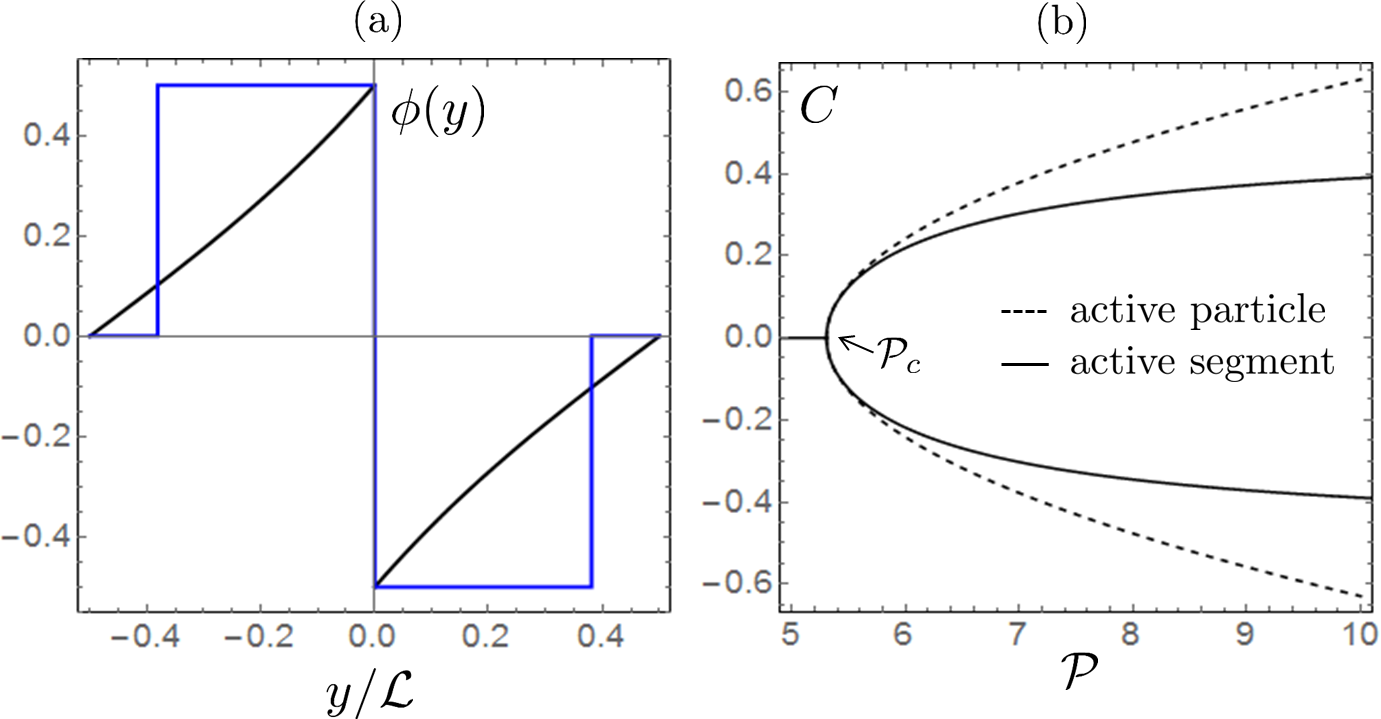
Figure 1: (a) Two AS models with different interaction kernels $\phi(y)$: black line is the exponential kernel introduced in Recho et al. (2015) and used in this paper and blue line is the kernel used in Kruse and Jülicher (2000). (b) Spontaneous polarization in AS and AP models when $\mathcal{P}$ increases above $\mathcal{P}_{c}$. Parameters: $F=0$, $\mathcal{L}=2$.

Suppose now that the internal configuration of the motors $c(y,t)$ is not observable and that we have access only to some global polarity measure $C(t)=\left\{\phi\ast c\right\}/\mathcal{L}\in[-\max\phi,\max\phi]$, where $\left\{h\right\}=(h|_{\mathcal{L}/2}+h|_{-\mathcal{L}/2})/2$. To obtain a closed description of the cell dynamics in terms of the ‘macro-variables’ $C(t)$ and $S(t)$, we need to map the AS model (1)–(2) onto an AP model.

To this end, we first average (2) in two different ways. Using the impenetrability condition we have $\dot{S}=\mathcal{P}C+F\left\{\phi\ast\partial_{y}f\right\}$ and by integrating (2) over space we obtain $\langle v\rangle=-\dot{S}+F/\mathcal{L}$. To eliminate the new macroscopic variable $\langle v\rangle$ we mimic (1) by writing $\dot{C}+\langle v\rangle=-\Phi(C)$. Here, the term $\langle v\rangle$ can be viewed as the analog of the drift term in (1), in particular, it ensures that a retrograde flow with $\langle v\rangle<0$ contributes to the growth of polarity. The term on the right-hand side is intended to play the role of diffusion degrading the existing polarity and therefore the function $\Phi$ is chosen to be increasing and vanishing at $C=0$. We obtain the closed nonlinear system of ordinary differential equations:

$$\dot{S}=\mathcal{P}C+k_{S}F,\,\ \dot{C}=\mathcal{P}C+k_{C}F-\Phi(C),$$ (3)

where $k_{S}=\left\{\phi\ast\partial_{y}f\right\}$ and $k_{C}=k_{S}-1/\mathcal{L}$. Note that the AP model (3) is non-potential because the cell position depends on its polarity while the reverse effect is absent. To relate the AP and AS models quantitatively we need to find a relation between the functions $\phi(y)$ and $\Phi(C)$.

For determinacy, we choose from now on to work with a particular AS model describing a contracting active gel on a solid background Bois et al. (2011); Recho et al. (2014) which is characterized by the kernel: $\phi(y)=\text{sh}\left(y+\mathcal{L}/2\right)/\left[2\text{sh}(\mathcal{L}/2)\right]-H(y)\text{ch}\left(y\right)$, where $H(y)$ is the Heaviside function, see Fig. 1 (a) and SI for details. To find a matching function $\Phi(C)$, it is sufficient to consider the case $F=0$.

Under these conditions, when the contractility parameter $\mathcal{P}$ in the AS model increases above a critical threshold $\mathcal{P}_{c}(\mathcal{L})$, the symmetric homogeneous solution of (1)–(2) $v=0$, $c\equiv 1$ and $V=0$ becomes unstable and a polarized motile state emerges as a result of pitchfork bifurcation (second order phase transition) leading to two symmetric configurations with opposite polarities, see Recho et al. (2014); SI and Fig. 1 (b).

To reproduce the same bifurcation in the framework of the AP model, we assume that $\Phi(C)=\partial_{C}\bar{W}$, where $\bar{W}(C)=\alpha C^{4}/4+\mathcal{P}_{c}C^{2}/2$ is the standard expression from the theory of second order phase transitions. At $F=0$ the polarity evolves according to the equation $\dot{C}=-\partial_{C}W$, where now $W(C)=\alpha C^{4}/4-(\mathcal{P}-\mathcal{P}_{c})C^{2}/2$ is the corresponding Landau potential. It has a single minimum at $C=0$ when $\mathcal{P}<\mathcal{P}_{c}$ and two symmetric minima at $C=\pm\sqrt{(\mathcal{P}-\mathcal{P}_{c})/\alpha}$ when $\mathcal{P}>\mathcal{P}_{c}$, see Fig. 1 (b). The coefficient $\alpha$ can be fixed by matching the asymptotic behavior for the two models at $\mathcal{P}=\mathcal{P}_{c}$. From a normal form analysis of the AS model, we obtain $\alpha=\mathcal{P}_{c}^{2}\mathcal{L}^{3}\theta_{2}(\mathcal{L})/2$ where the analytical expression for the function $\theta_{2}(\mathcal{L})>0$ is given in SI .

To test the efficiency of our calibration procedure, we now subject both systems, AS and AP, to a fixed external force and compare the resulting velocity-force (V-F) relations for steady regimes. In the AS framework, for simplicity, we will deal with the case when where the external force is shared by the two boundaries of the segment: $f(y,t)=\beta\delta(y+\mathcal{L}/2)+(1-\beta)\delta(y-\mathcal{L}/2)$ where the value of $\beta$ is irrelevant in what follows because of the fixed length constraint. For the corresponding AP model we obtain $k_{S}(\mathcal{L})=(1/2)\coth(\mathcal{L}/2)>0$.

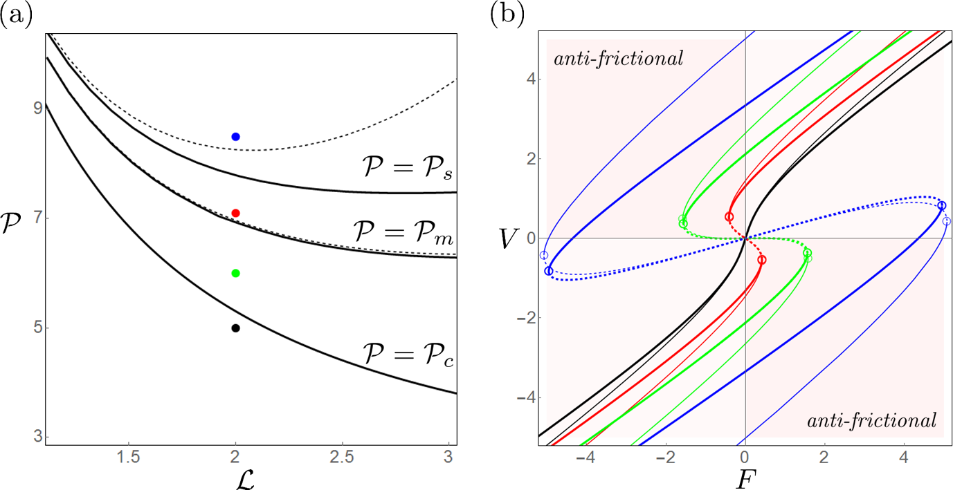
Figure 2: Comparison of the V-F relations in AS and AP models. (a) The three thresholds $\mathcal{P}_{c}$, $\mathcal{P}_{m}$ and $\mathcal{P}_{s}$ as functions of the parameter $\mathcal{L}$. Thick lines - AS model, dotted lines - AP model. The value of $\mathcal{P}_{c}$ is the same in both models by construction. (b) Four typical V-F relations in the AS (thick lines) and the AP (thin lines) models. The dashed parts of the V-F curves correspond to unstable regimes. Parameters $\mathcal{L}=2$ and $\mathcal{P}={\color[rgb]{0,0,0}5}$ (black), $\mathcal{P}=6$ (red), $\mathcal{P}=7$ (green) and $\mathcal{P}=9$ (blue) are represented with color dots on panel (a).

In the case of the AS model, we solve numerically equations (1)–(2) with $\partial_{t}c=0$. In the AP setting we find the stationary value of polarity $C$ directly from the equation $\partial_{C}W=k_{C}F$ and then obtain the V-F relation substituting this value of $C$ into (3). As shown on Fig. 2 (b), both models generate quantitatively similar V-F relations in the whole range of parameters.

When $\mathcal{P}<\mathcal{P}_{c}$, the V-F relations in both models are single-valued and frictional, meaning that $VF>0$. This is obvious in the AP case since the potential $W(C)$ is convex and the system has only one stable ($\partial_{CC}W(C_{0})>0$) stationary solution $C_{0}(F)$. The ensuing V-F relation can be written explicitly $V=k_{S}F+\mathcal{P}C_{0}(F)$. Note that due to the presence of motors, the effective viscosity in the active system $\mu_{0}=\partial_{V}F|_{V=0}=(\mathcal{P}_{c}-\mathcal{P})/(k_{S}\mathcal{P}_{c}-\mathcal{P}/\mathcal{L})$ is smaller than in its passive analog ($\mathcal{P}=0$) and can even reach zero, which is a feature of many active systems Haines et al. (2008); López et al. (2015). A similar but less explicit analysis can be performed for the AS model, see SI .

When $\mathcal{P}>\mathcal{P}_{c}$, the V-F curves develop a domain of bi-stability which spreads over a range $F\in[-F_{t},F_{t}]$, where, in the AP model, $F_{t}=2(\mathcal{P}-\mathcal{P}_{c})^{3/2}/(3k_{C}\sqrt{3\alpha})$. Within this range, the stationary polarity can take three values: $C_{0}^{*}<C_{0}<C_{0}^{**}$ where $C_{0}^{*}<0<C_{0}^{**}$ correspond to metastable solutions and $C_{0}$ is an unstable solution ($\partial_{CC}W(C_{0})<0$). In this range, the V-F relations allow for the coexistence of the two metastable regimes with different signs of velocity: $V^{*}=k_{S}F+\mathcal{P}C_{0}^{*}(F)$ and $V^{**}=k_{S}F+\mathcal{P}C_{0}^{**}(F)$. These two branches of the V-F relation are connected by the unstable branch $V_{0}=k_{S}F+\mathcal{P}C_{0}(F)$, which is located between the two turning points $F=\pm F_{t}$. Inside the coexistence interval $[-F_{t},F_{t}]$, one of the two metastable solutions necessarily operates in an anti-frictional regime with $VF\leq 0$ SI . Similar bi-directionality with negative viscosity at zero force, is also characteristic of the V-F curves describing an ensemble of molecular motors interacting either hydrodynamically Malgaretti et al. (2017) or through a rigid backbone Jülicher and Prost (1995).

A new feature of the model is the existence of another threshold, $\mathcal{P}_{m}$ ($=k_{S}\mathcal{L}\mathcal{P}_{c}$ in the AP case), beyond which the zero velocity regime stabilizes, the viscosity at zero force becomes positive again and the V-F curves start to display muscle-like stall force states. For $\mathcal{P}_{m}<\mathcal{P}<\mathcal{P}_{s}$, where $\mathcal{P}_{s}=2k_{S}\mathcal{P}_{c}/(3/\mathcal{L}-k_{S})$ in the AP case, such states are unstable but for $\mathcal{P}>\mathcal{P}_{s}(\mathcal{L})$ they stabilize. The functions $\mathcal{P}_{m,s}(\mathcal{L})$ for the AS model are compared with those for the AP model in Fig. 2(a) and the corresponding V-F curves can be read off Fig. 2(b).

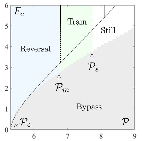
Figure 3: Phase diagram showing the four robust outcomes of the collision test: Reversal, Train and Pairing of cells which splits into a motile phase (Train) and a static one (Still). Typical dynamics are illustrated on Fig. 4. Parameters are $\mathcal{L}=2$ and $\mathcal{D}_{c}=0.1$. Coloring corresponds to the AS model while dashed lines are for the AP model.

Consider now two identical cells moving towards each other. The cells will be represented either as AS or AP and we shall use the subscripts $-$ and $+$ to differentiate between cells approaching from the left and from the right. We assume that the colliding cells have to overcome the repulsive force

$$F_{\pm}(\mathcal{D})=\pm F_{c}\exp(-\mathcal{D}/\mathcal{D}_{c}),$$ (4)

which depends on the separation: $\mathcal{D}(t)=|x_{r_{+}}(t)-x_{f_{-}}(t)|$ for the AS model and $\mathcal{D}(t)=|S_{+}(t)-S_{-}(t)|$ for the AP model. Note that we introduce a characteristic size of a cell-cell contact $\mathcal{D}_{c}\ll\mathcal{L}$ and define $F_{c}$ as the scale of the repulsive force. We also implicitly assume that the adhesive clusters are only transient and cannot support significant tensile loads Stramer and Mayor (2017).

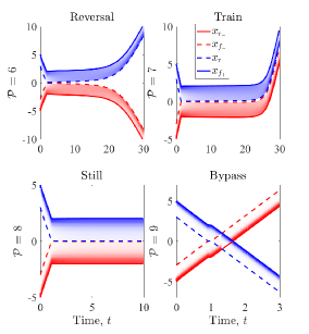
Figure 4: The configurations of two colliding cells obtained within the AS model (1,2) with the contact force (4). The intensity of the coloring between the front lines is proportional to the concentration of molecular motors. Parameters: $\mathcal{L}=2$, $\mathcal{D}_{c}=0.1$ and $F_{c}=4.5$.

In our simulations we explore the whole range $\mathcal{P}>\mathcal{P}_{c}$. Similar to what is observed in experiment Desai et al. (2013); Scarpa et al. (2013) and predicted based on a much more detailed model Kulawiak et al. (2016), we record four possible outcomes of collision tests: reversal, paring, which can be motile (train) or static (still), and bypass. Our results are presented in the $(\mathcal{P},F_{c})$ phase diagram shown for both AS and AP models in Fig. 3.

In the reversal regimes, the active objects re-polarize during collision as a result of being exposed to sufficiently large contact force. The outcome of such ‘quasi-elastic’ collision is that the colliding agents change the signs but not the magnitudes of their velocities. In the bypass regimes, the agents go past each other because the model allows for mutual overlap and the contact force is not sufficient to impede the propulsive machinery. In the pairing regimes the two initially mobile agents first get immobilized and push against each other as both of them reach transiently stall conditions. Such regimes can be stable (forming a robust still phase) only for $\mathcal{P}>\mathcal{P}_{s}$ where a steady stall state exists. For $\mathcal{P}<\mathcal{P}_{s}$, in the train regimes, one of the two active agents eventually sweeps along the other by repolarizing its internal configuration and afterwards they continue traveling together as a cell doublet (train). In these regimes, stall configurations do exist but are unstable and are destroyed by infinitesimal perturbations, see SI for details. Note however that the exact partitioning of the pairing phase into still and train regimes is somewhat arbitrary since we did not specify the attractive/cohesive structure of the interaction model.

The typical trajectories of the colliding active agents for each of the four regimes and the corresponding configurations of molecular motors in the AS and AP models are illustrated in Fig. 4 and Fig. 5. Remarkably, both models show a qualitatively similar behavior. In the AP case, we also represent the transient collision trajectories $(F_{\pm}(t),\dot{S}_{\pm}(t))$ on the V-F plane where they can be compared with the stationary V-F relations. The two types of curves deviate because, in collision tests, polarity does not relax instantaneously to its steady value; moreover the interaction force itself varies during such relaxation. The finite time of relaxation is particularly important for the existence of train regimes which crucially rely on the ability of active agents to transiently reach an unstable stall state.

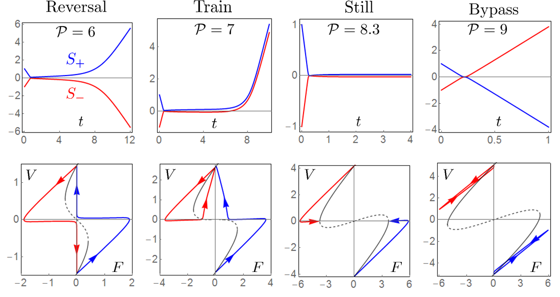
Figure 5: Four typical collision scenarios observed in the AP model. The first row shows the trajectories of the colliding particles. The second row illustrates the transient velocity-force dynamics superimposed on the steady V-F relation. Parameters: $\mathcal{L}=2$, $F_{c}=6$ and $\mathcal{D}_{c}=0.1$

To conclude, we have used a one-dimensional model of contraction-driven cell motility to develop an equivalent active particle model spontaneously adjusting its polarity to the applied force. Both models are able to predict the outcomes of collision tests covering the whole spectrum of observed behaviors. An important prediction is that cell contractility serves as the key internal regulator of CIL which could be further investigated experimentally by using drug treatments Mitrossilis et al. (2009) or optogenetics Valon et al. (2017). The proposed model of active particle with self-adjusting polarity is capable of describing complex mechanical cell-cell interactions and can prove useful for the development of a kinetic theory of tissues driven by internal cellular motion.