Structural transition of vortices to nonlinear regimes in a dusty plasma

Abstract

A 2D hydrodynamical model is developed and analyzed for the steady state of a driven-dissipative dust clouds confined in an azimuthally symmetric toroidal system which is in dynamic equilibrium with background unbounded streaming plasma. Its numerical solution not only confirms the analytical structure of the driven dust vortex flow in linear limit as reported in previous analysis, but also shows how the dust vortices are strongly affected by the nonlinear convection of the flow itself. Effects of various system parameters including external driving field and Reynolds number (Re) are investigated within the linear to nonlinear transition regime $0.001\leq{\rm Re}<50$. In agreement with various relevant experimental observations, the flow structure which is symmetric around center in the linear regime begins to turn asymmetric in the nonlinear regime. The equilibrium structure of dust flow is found to be influenced mainly by the dissipation scales due to kinematic viscosity, ion drag, and neutral collision in the nonlinear regime, whereas in the linear regime, it is mainly controlled by the external driving field and the confining boundaries.

I Introduction

Vortex or swirling flows about an axis are ubiquitous in most complex fluids involving multiple spacial and temporal scales. The key feature of such complex fluids is the interactions of various constituents that lead to collective behaviors such as self-organization and pattern formation Holzer et al. (2010); Grossmann (2000); Laishram et al. (2015, 2014). For examples, flows in polymer solutions, colloidal suspensions and many biological systems are complex flows in low Reynolds number regimes that exhibit vortex or circulating flow pattern Lauga and Powers (2008); Wolgemuth (2008); Pan et al. (2013); Yager and H. (2006); Squires and Quake (2005); Stroock et al. (2002). On the other hand, similar self-organized vortex flows are also observed in many higher Reynolds number macroscopic flow systems such as White Ovals, Great Red Spot of Jupiter, polar vortex of Earth, and macroscopic circulations including hurricanes and tornadoes in planetary atmospheres Sommeria and L. (1988); Choi et al. (2007); Marcus (1990). The vortex structure in such driven dissipative systems evolves in various dynamical regimes. It has been observed in different sizes, shapes, orientations, aspect ratios, and convection velocities. It has been recognized that vortex structure plays an important role in fluid mixing and transport process in laminar and turbulent flows Nivedita (2017); Marcus (1990). Thus it has been a topic of active research that how the vortical structure evolution in various complex fluid flows depends on system parameters, in particular the Reynolds number from the viscous dominant linear regime to inertial dominant nonlinear flow regime. When the flow is viscous dominant which happen mostly at lower flow velocity and smaller length scale (Re$\leq 1$), the gradients in the hydrostatic pressure are balanced by viscous diffusive producing smooth deformation and laminar flows. However, at higher flow velocity and larger length scale (Re$\gg 1$), the viscous stress is comparable or less than the inertial convective transport and the pressure gradients act to accelerate the fluid elements and generate nonlinear convective flows.

Interestingly, dust clouds electrostatically suspended in a plasma can be a realizable prototype for experimental or theoretical formulation for various characteristics of driven-dissipative complex fluid flows. Dusty plasmas with coupling parameters in the ranges of $10\leq\Gamma\leq 100$ for a fixed screening parameter $\kappa$ behave like complex fluids. They can form many self-organized vortices or circulating flow as collective behaviors due to its long-range Coulomb interactions Fortov et al. (2003); Morfill et al. (1999). Here $\Gamma=E_{p}/E_{k}$, i.e., the strength of Coulomb potential energy $E_{p}$ over kinetic energy $E_{k}$ and the screening parameter $\kappa=d/\lambda_{D}$, i.e., the ratio of the particle distance over the Debye length due to background plasma  Thomas et al. (1994); Morfill et al. (1999). Study of dust vortex structures in such a complex plasma presents an attractive option for analyzing and interpreting the dynamics of many relevant complex fluid flows in laboratories, industrial applications as well as many natural processes. In the previous linear (Re$\ll 1$) analysis Laishram et al. (2015, 2014), the analytic structure of the steady dust flow driven by an unbounded and sheared ion flow is obtained. The scales of the vortex developed in linear regime mainly depend on those of the ion flow driver, the boundaries, and as various system parameters including the kinematic viscosity. In recent dusty plasma experiments Kaur et al. (2015a, b), a very localized and isolated regions of acceleration and frictional retardation in velocity field, along with an uniform vorticity region surrounded by highly sheared layers of dust vortex motion are produced. This suggests that the laboratory dusty plasma may have entered the nonlinear regime of the vortex flow and lends itself to the study of macroscopic nonlinear dynamics in such systems of similar Reynolds number Laishram et al. (2015). It motivates us to extend the previous linear analysis to higher Reynolds number flow regime (Re$\gg 1$), where the nonlinear inertial flow is effective which may explain many new flow characteristics as observed in dusty plasma experiments Kaur et al. (2015a).

In present work, we employ a 2D numerical model for the dynamics of a steady isothermal dust fluid confined in an axisymmetric toroidal configuration in dynamical equilibrium with an unbounded sheared flow of a streaming ions through a combination of electrostatic and gravitational fields. This model is very general and is applicable to any driven dissipative systems in arbitrary Reynolds number flow regimes. The dust fluid is assumed to be incompressible, viscous, and Newtonian, in which the dust is dragged by the shear streaming of ions through the confined domain. In such a system where an external momentum source is present, specific steady flow solutions are attainable only in presence of a frictional sink of momentum which is afforded by the stationary background plasma and neutral fluids. The main objective of present work is to understand the characteristics of dust flow in presence of inertial flow at higher Reynolds number regimes and the corresponding changes in vortex structure from linear to nonlinear flow regimes.

The manuscript is organized as follows. The 2D hydrodynamic model and numerical methods for studying the dynamics of driven-dissipative dust fluid for arbitrary Re in a toroidal configuration are introduced in Sec. II. Then a detailed characterizations of the steady dust flow structures in linear and nonlinear regime are discussed in Sec. III. The nonlinear effects on the vortex structure with varying system parameters, namely, the external driving field, the kinetic viscosity of the dust fluid $\mu$, the ion dragging co-efficient $\xi$, and the neutral collision frequency $\nu$ are described in Sec. III.2 and Sec. III.3 respectively. Summary and conclusions are presented in Sec. IV.

II Hydrodynamic model and numerical method

The geometry of confined dust fluid is taken from the recent experiment where a toroidal dust cloud flowing in poloidal direction in a glow discharge plasma, as shown in Fig. 1(a) Kaur et al. (2015b, a). The confinement and localization of the dust clouds in these and similar laboratory experiments are achieved effectively by a combination of electrostatic and gravitational fields, where a 2D or 3D conservative field ${\bf F_{c}}=-\nabla V_{b}$ is prepared with various experimental means Klindworth et al. (2000); Mitic et al. (2008a); Fink et al. (2013); Arp et al. (2005).

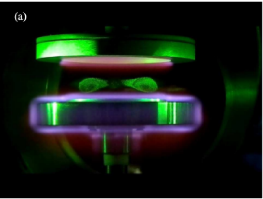
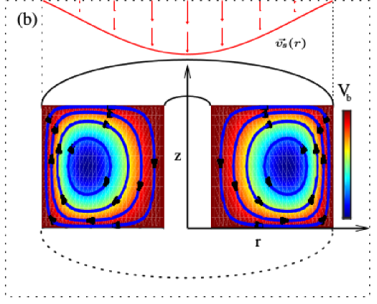
Figure 1: (a) Toroidal dust clouds with poloidal circulation in the laboratory dusty plasma experimental setup by M. Kaur et  al. Kaur et al. (2015a). (b) Schematic representation of dust cloud confined toroidally by the electrostatic potential ${V_{b}(r,z)}$ and driven poloidally by the sheared ion flow $\upsilon_{s}(r,z)$ through out the dust clouds [Reprinted courtesy of AIP Conference Proceedings 1925, 020028 (2018) by permission]

The dust fills the volume of the torus where the shape of its poloidal cross-section is determined by the effective confining potential. However, for the computational simplicity, the system in present model is approximated as being axisymmetric and the poloidal cross-section of the torus is simplified as a rectangle as illustrated schematically in Fig 1(b). The toroidal dust fluid is considered confined by an effective potential $V_{b}(r,z)$ within the boundaries of a finite section of an infinitely long cylinder of flowing plasma, where $0<r/L_{r}<1$, $-1<z/L_{z}<1$, and $0<\phi<2\pi$. The effective confining potential ${V_{b}(r,z)}$ jumps from a small value within the domain to a very high value at the rectangular boundary, which serves as a rectangular equipotential line for the boundary condition of a perfect confinement.

For the dust flow that satisfies incompressible and isothermal conditions and has a finite viscosity, the dynamics is governed by the simplified Navier-Stokes equations in which the drive produced by the sheared ion drag and the friction produced by the stationary background neutral fluid can be accounted for non-conservative vorticity sources Landau and Lifshitz (2013),

$$\frac{\partial{\bf u}}{\partial t}+({\bf u}\cdot\nabla){\bf u}=-\frac{\nabla{P}}{\rho}-\nabla{V}+\mu\nabla^{2}{\bf u}\hskip 39.83368pt$$

$$-\xi({\bf u}-{\bf v})-\nu({\bf u}-{\bf w}).$$ (1)

Here ${\bf u}$, ${\bf v}$ and ${\bf w}$ are the flow velocities of the dust, ion, and neutral fluids, respectively. $P$ and $\rho$ are the pressure and mass density of the dust fluid, respectively, $V(r,z)$ is the confining potential, $\mu$ is the kinematic viscosity, $\xi$ is the coefficient of ion drag acting on the dust, and $\nu$ is the coefficient of friction generated by the stationary neutral fluid Barnes et al. (1992); Khrapak et al. (2002); Ivlev et al. (2004). The overall combination of charged dust and background plasma is quasi-neutral and the electrons are in thermal equilibrium with the streaming ions and the confined dust. The incompressibility condition of the confined dust fluid

$$\nabla\cdot{\bf u}=0,$$ (2)

defines a potential called stream function ${\Psi}$ such that ${\bf u}=\nabla\times{\Psi}$. In case of an azimuthally symmetric dust flow the dust motion can suitably be treated in the 2-dimensional $r$-$z$ plane where the dust vorticity vector $\vec{\omega}=\nabla\times{\bf u}$ is in the toroidal direction only. Then the stream function becomes like a scalar field for two dimensional flows giving ${\bf u}=\nabla\times(\psi\hat{\phi})$. For a stationary background neutral fluid (${\bf w}=0$), the equations for the two-dimensional steady dust flow can be derived from Eqs. (1)-(2) as follows,

$$\nabla^{2}\psi = -\omega,$$ (3)

$$({\bf u}\cdot\nabla){\omega} = \mu\nabla^{2}\omega-(\xi+\nu)\omega+\xi\omega_{s},$$ (4)

where $\omega_{s}$ is the external vorticity source from the unbounded sheared ion flow. The 2D solutions of (3)-(4) were recently obtained in the linear regime (Re$<1$), where the inertial effects are dominated by the diffusive transport and thus the nonlinear term in the left-hand side of the momentum equation can be ignored in the linear viscous limit Laishram et al. (2014, 2015). The Eqs. (4) in the linear limit admits standard solution procedures where integration is possible for an individual mode of the dust vorticity interacting with that of the driver. As presented in Ref. Laishram et al. (2014, 2015), such 2D linear solutions are obtained by constructing an eigenvalue problem and representing the dust and source stream function in terms of a set of orthogonal eigenfunctions that satisfy the appropriate boundary conditions. In nonlinear regime, the equations can be solved using proper numerical approach. Here the method of Successive Over Relaxation (SOR) Press (1992) is adopted in the present study.

In the first step, the Eqs. (3) and Eqs. (4) are normalized using proper scaling units $L_{r}$ and $U_{0}$ etc, such that the $\psi\rightarrow\psi/[U_{0}L_{r}]$, $\omega\rightarrow\omega/[U_{0}/L_{r}]$, ${\bf u}\rightarrow{\bf u}/[U_{0}]$, $\omega_{s}\rightarrow\omega_{s}/[U_{0}/L_{r}]$, $\mu\rightarrow\mu/[U_{0}L_{r}]$, $\xi\rightarrow\xi/[U_{0}/L_{r}]$, and $\nu\rightarrow\nu/[U_{0}/L_{r}]$, etc. Then the relative importance of various terms in the equation can be compared in terms of the magnitude of the dimensionless coefficients. Now, in normalized dimensionless form, the 2-D steady incompressible N-S equations for the dust fluid can be written as

$$0 = \nabla^{2}\psi+\omega,$$ (5)

$$0 = \nabla^{2}\omega-\frac{1}{\mu}({\bf u}\cdot\nabla){\omega}-\frac{(\xi+\nu)}{\mu}\omega+\frac{\xi}{\mu}\omega_{s}.$$ (6)

Then the equations are cast in the form suitable for numerical solutions. Using cylindrical coordinates $(r,\phi,z)$ and assuming axisymmetry, Eqs. (5) and (6) can be solved in iterative steps,

$$\psi^{n+1}=\psi^{n}+\Delta L^{2}\left(\frac{\partial^{2}}{\partial r^{2}}+\frac{1}{r}\frac{\partial}{\partial r}-\frac{1}{r^{2}}+\frac{\partial^{2}}{\partial z^{2}}\right)\psi^{n}$$

$$+{\Delta L^{2}}\omega^{n},$$ (7)

$$\omega^{n+1}=\omega^{n}+\Delta L^{2}\left(\frac{\partial^{2}}{\partial r^{2}}+\frac{1}{r}\frac{\partial}{\partial r}-\frac{1}{r^{2}}+\frac{\partial^{2}}{\partial z^{2}}\right)\omega^{n}$$

$$-\frac{\Delta L^{2}}{\mu}\left(u_{r}\frac{\partial\omega}{\partial r}\right)^{n}-\frac{\Delta L^{2}}{\mu}\left(u_{z}\frac{\partial\omega}{\partial z}\right)^{n}$$

$$-{\Delta L^{2}}K_{1}\omega^{n}+{\Delta L^{2}}K_{2}\omega_{s},$$ (8)

where $\Delta\psi\equiv\psi^{n+1}-\psi^{n}$ is iterative variation, ${\Delta L}$ is the iteration step size (or virtual time step size), $K_{1}=(\xi+\nu)/\mu$, $K_{2}=\xi/\mu$, and $n$ represents the iteration step. Since $\psi^{n+1}\rightarrow\psi^{n}$ for the steady state, the above equations can be rearranged as follows,

$$\left[1-\Delta L^{2}\left(\frac{\partial^{2}}{\partial r^{2}}+\frac{1}{r}\frac{\partial}{\partial r}+\frac{\partial^{2}}{\partial z^{2}}\right)\right]\psi^{n+1}=\psi^{n}$$

$$+{\Delta L^{2}}\omega^{n}-\frac{\Delta L^{2}}{r^{2}}\psi^{n},$$ (9)

$$\left[1-\Delta L^{2}\left(\frac{\partial^{2}}{\partial r^{2}}+\frac{1}{r}\frac{\partial}{\partial r}+\frac{\partial^{2}}{\partial z^{2}}\right)\right]\omega^{n+1}=\omega^{n}$$

$$-\frac{\Delta L^{2}}{\mu}\left(u_{r}\frac{\partial\omega}{\partial r}\right)^{n}-\frac{\Delta L^{2}}{\mu}\left(u_{z}\frac{\partial\omega}{\partial z}\right)^{n}$$

$$-\frac{\Delta L^{2}}{r^{2}}\omega^{n}-{\Delta L^{2}}K_{1}\omega^{n}+{\Delta L^{2}}K_{2}\omega_{s}.$$ (10)

For numerical efficiency, the above equations are rewritten in a two-operator form where each operator has only one directional derivative as follows,

$$\left[1-\Delta L^{2}\left(\frac{\partial^{2}}{\partial r^{2}}+\frac{1}{r}\frac{\partial}{\partial r}\right)\right]\left[1-\Delta L^{2}\frac{\partial^{2}}{\partial z^{2}}\right]\psi^{n+1}$$

$$=\psi^{n}+{\Delta L^{2}}\omega^{n}-\frac{\Delta L^{2}}{r^{2}}\psi^{n}$$

$$+\Delta L^{4}\left(\frac{\partial^{2}}{\partial r^{2}}+\frac{1}{r}\frac{\partial}{\partial r}\right)\left(\frac{\partial^{2}}{\partial z^{2}}\right)\psi^{n},$$ (11)

$$\left[1-\Delta L^{2}\left(\frac{\partial^{2}}{\partial r^{2}}+\frac{1}{r}\frac{\partial}{\partial r}+\frac{1}{\mu}{\frac{\partial\psi^{n}}{\partial z}}\frac{\partial}{\partial r}\right)\right]\left[1-\Delta L^{2}\left(\frac{\partial^{2}}{\partial z^{2}}\right.\right.$$

$$\left.\left.-\frac{1}{\mu}\left(\frac{\partial\psi^{n}}{\partial r}+\frac{\psi^{n}}{r}\right)\frac{\partial}{\partial z}\right)\right]\omega^{n+1}=\omega^{n}-\left(\frac{\Delta L^{2}}{r^{2}}\right)\omega^{n}$$

$$-{\Delta L^{2}}K_{1}\omega^{n}+{\Delta L^{2}}K_{2}\omega_{s}^{n}$$

$$+\Delta L^{4}\left(\frac{\partial^{2}}{\partial r^{2}}+\frac{1}{r}\frac{\partial}{\partial r}+\frac{1}{\mu}{\frac{\partial\psi^{n}}{\partial z}}\frac{\partial}{\partial r}\right)$$

$$\left(\frac{\partial^{2}}{\partial z^{2}}-\frac{1}{\mu}\left(\frac{\partial\psi^{n}}{\partial r}+\frac{\psi^{n}}{r}\right)\frac{\partial}{\partial z}\right)\omega^{n}.$$ (12)

In order to compute the solutions on a two dimensional grid, an initial guess on $\psi_{ij}^{1}$ and $\omega_{ij}^{1}$ is made for stream function and vorticity respectively, by additionally imposing the desired boundary conditions. In each iteration with index $n$, beginning from $n=1$, Eq. (11) is first solved for the radial operator part (i.e., r-part) on $A_{ij}^{n+1}$, which formally represents the result of the second factor in the LHS of Eq. (11) operating on the updated stream function $\psi^{n+1}$,

$$\left[1-\Delta L^{2}\frac{\partial^{2}}{\partial z^{2}}\right]\psi_{ij}^{n+1}=A_{ij}^{n+1}.$$ (13)

The values of the computed radial operator part $A_{ij}^{n+1}$ allow the determination of $\psi_{ij}^{n+1}$ by inverting the axial operator part (i.e., z-part) in Eq. (13). The advantage of this process is that the above equations (11) and (13) are reduced to tridiagonal systems which is numerically more efficient Press (1992).

An identical procedure is applied for determining $\omega_{ij}^{n+1}$ by defining

$$\left[1-\Delta L^{2}\left(\frac{\partial^{2}}{\partial z^{2}}-\frac{1}{\mu}\left(\frac{\partial\psi^{n}}{\partial r}+\frac{\psi^{n}}{r}\right)\frac{\partial}{\partial z}\right)\right]\omega_{ij}^{n+1}=B_{ij}^{n+1}.$$ (14)

Then Eq. (12) is first solved for $B_{ij}^{n+1}$, which allows Eq. (14) to be solved for $\omega_{ij}^{n+1}$. The updated $\psi_{ij}^{n+1}$ values are used in second half of the iteration to compute $B_{ij}^{n+1}$ and $\omega_{ij}^{n+1}$, rather than the old values $\psi_{ij}^{n}$, which concludes the $n^{\rm th}$ iteration. The iterations are made updating the $\omega$ and $\psi$ fields until the minimum values of the residues $R_{1}(=\frac{\Delta\psi}{\Delta L^{2}})$ and $R_{2}(=\frac{\Delta\omega}{\Delta L^{2}})$ below a reasonably small tolerance are achieved. The relative change in errors define by $Error=max(|\frac{\omega^{n+1}-\omega^{n}}{\omega^{n}}|)$ decreases in each iterative step down to the tolerance limit ($10^{-6}$), which ensures the convergence to a steady state solution as shown in Fig 2. The iteration step ${\Delta L}$, grid size $\Delta r$, and kinematic viscosity $\mu$ are the main parameters that affect the speed of convergence and numerical stability.

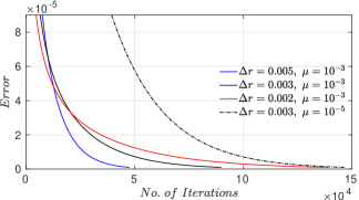
Figure 2: Relative error as a function of iterative steps near the tolerance limit of $10^{-6}$ for various grid size $\Delta r[L_{r}]$ and kinematic viscosity $\mu[U_{0}L_{r}]$.

III Characterization of steady equilibrium dust flow structure.

The above equations are solved subject to proper boundary conditions. The boundary for the dust flow in the present treatment is defined by the effective potential that allows no dust flow across the confined domain where the potential $V_{b}$ for dust jumps from a small accessible value to a large value at boundaries. This confinement property($u_{\perp}=0$) at the boundary gives the boundary conditions for stream function say $\psi_{wall}=0$. The boundary condition for $\omega_{wall}$ depends on the nature of $u_{\parallel}$ of the confined dust flows. A perfect slip, partial slip, and no slip are some of the common boundary conditions for $u_{\parallel}$. The difficulty with a vorticity stream function formulation is the lack of natural boundary conditions in term of vorticity $~{}\omega_{wall}$, which however can be derived approximately using Thom’s formula Weinan and Liu (1996).

For easy comparison with the analytic solutions presented in Laishram et al. (2014, 2015), we have used the identical conditions as the typical laboratory glow discharge argon plasma with micron-sized dust. The plasma parameters are $n\simeq 10^{9}$ cm^-3, $T_{e}\simeq 3eV$, and $T_{i}\simeq 1eV$ largely at the sheath entrance where ions are streaming with a flow velocity $U_{0}$ at the order of the ion acoustic velocity $c_{s}=\sqrt{T_{e}/m_{i}}$. Further, using the radial width of the confined domain $L_{r}$ and steaming ions velocity $U_{0}$ as the ideal normalization units for the lengths and velocity of the dust flow system, the value of ion drag coefficient can be estimated as $\xi\sim 10^{-5}~{}[U_{0}/L_{r}]$ and the neutral collision frequency as $\nu\sim 10^{-1}~{}[U_{0}/L_{r}]$ Barnes et al. (1992); Khrapak et al. (2002); Ivlev et al. (2004). For a typical system size, $L_{r}\sim 10~{}cm$, the range of kinematic viscosity $\mu$ can similarly be chosen as $\mu\sim 10^{-6}~{}[U_{0}L_{r}]$ which corresponds to the small Reynolds numbers (Re$~{}\approx 1$) of the dust flow in the linear viscous regime Laishram et al. (2015).

III.1 Benchmark of the numerical solutions

The present model for dust clouds is generic and and applicable to many driven-dissipative dynamic equilibrium system. It has the freedom of choice for external driver, i.e., the background ions flow, and the boundary of confining domain. However, for direct comparison with the previous analytic solutions Laishram et al. (2015), now we consider the same physical conditions, especially the same external driving field. The flow profile of streaming ions is specified as,

$$v_{z}(r,z)=A_{m}J_{0}\left(\alpha_{I}\frac{r}{L_{r}}\right)\cos{\left(\frac{\pi z}{2L_{z}}\right)}.$$ (15)

Here $A_{m}$ is the magnitude of external driving field. The radial modes are determined by the $I_{th}$ root of Bessel function $J_{0}(\alpha_{I})=0$ at the external boundary. The axial mode $k_{z}=(\pi/{2L_{z}})$ specifies a single vortex along axial direction as in experimental observations Kaur et al. (2015a). The numerical solution for the stream function $\psi(r,z)$ and its corresponding streamlines ( i.e., the contours of the product $r\psi$) in the linear viscous regime are shown in Fig. 3(b)-(c) respectively for $\mu=10^{-3}[U_{0}L_{r}]$, $\xi=10^{-5}[U_{0}/L_{r}]$ and $\nu=10^{-1}[U_{0}/L_{r}]$.

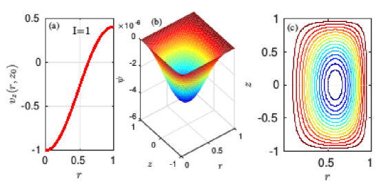
Figure 3: (a) Driver ion velocity flow profile $v_{z}(r,z)$ with axial and radial shear at $z=z_{0}$ cross-section, (b) 2D stream function $\psi(r,z)$ of the dust flow, and (c) Corresponding streamlines for the dust fluid flow in $r-z$ crossection for system parameters $\mu=~{}1\times 10^{-3}[U_{0}L_{r}]$, $\xi=~{}1\times 10^{-5}[U_{0}/L_{r}]$ and $\nu=~{}1\times 10^{-1}[U_{0}/L_{r}]$.

This streamline pattern shows similar characteristic features of low-Re dust flow as in Laishram et al. (2015), where the flow is anti-clockwise circulation, axial symmetric and aligned to the confining boundary, ensuring vorticity transport purely due to diffusion orthogonal to the streamlines.

A more quantitative comparison is possible between the flow velocity component profiles obtained numerically and those from analytic solutions in the linear limit Laishram et al. (2015). The profiles of the dust flow velocity components, i.e., $u_{z}(r,z_{0})$ and $u_{r}(r_{0},z)$ passing through the center of the circulation $(r_{0},z_{0})$ are compared for the kinematic viscosity varying from $\mu=10^{-1}~{}to~{}\mu=10^{-5}[U_{0}L_{r}]$ in the linear regime (Re$\ll 1$) (Fig. 4).

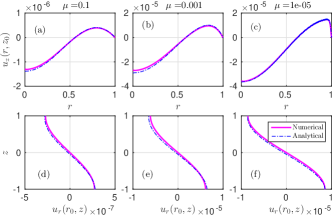
Figure 4: Comparison between analytical and numerical solutions of $u_{r}(r_{0},z)~{}and~{}u_{z}(r,z_{0})$ for fixed system parameters, $\xi=~{}1\times 10^{-5}[U_{0}/L_{r}]$, $\nu=~{}1\times 10^{-1}[U_{0}/L_{r}]$, and varying $\mu=~{}10^{-1}~{}to~{}10^{-5}[U_{0}L_{r}]$ in the linear regimes Re$\ll 1$.

In the highly viscous regimes, the dust fluid flows with a velocity in the range of $0.1-1~{}mm/sec$ in the confined domain. The analytical and numerical results are in good agreement. The above comparisons show the validity of the numerical method and motivates for further analysis of the driven dust flow characteristics at higher Reynolds number nonlinear regimes. Further, the variations in velocity profiles for $u_{r}(r_{0},z)$ and $u_{z}(r,z_{0})$ near the boundary indicates the impact of boundary conditions and the formation of boundary layer in particular. Boundary layers are formed due to the effective viscous stress on flow due to boundaries. The thickness of the boundary layer decreases with kinematic viscosity as shown in Fig. 4(a)-(c). Thus at higher Reynolds number, the thickness of boundary layer is negligibly small as $\Delta r_{b}\simeq\mu^{1/3}$ Laishram et al. (2015), and reduces to a very thin layer giving sharp deviation in velocity profile as shown in Fig. 4(f). There is no boundary layer formation for the perfect slip boundary conditions as shown in Fig. 4(d)-(f).

III.2 Emerging nonlinear characteristics in the steady equilibrium dust flow structures

When the contribution of nonlinear advection transport ${\bf(u\cdot\nabla)u}$ is included in the higher Reynolds number regimes, the momentum of dust flow increases enormously and it becomes important to maintain a low driver ion velocity so that Mach number of the dust $M_{d}=u_{d}/c_{sd}\ll 1$ for incompressible flow in practice. Thus, for the study of nonlinear effects at higher Re regimes, the driver ions stream with a shear flow velocity $U_{0}$ equivalent to a fraction of the ion acoustic speed $c_{s}$. The order of kinematic viscosity corresponding to small Reynolds numbers (Re$\simeq 1)$ of dust flow becomes $\mu\sim 10^{-4}~{}[U_{0}L_{r}]$ which is consistent with the linear viscous regime. The corresponding ion drag coefficient can be estimated as $\xi\sim 10^{-4}~{}[U_{0}/L_{r}]$, and neutral collision frequency as $\nu\sim 10^{-3}~{}[U_{0}/L_{r}]$ for further analysis Barnes et al. (1992); Khrapak et al. (2002); Ivlev et al. (2004).

Now the above flow analysis of the bounded driven dust flow dynamics is extended to high Re regimes. The streamlines of 2D steady dust flow in the linear and nonlinear regimes are presented in Fig. 5 for the radial mode numbers $I=1$ and $3$ of the same driver flow.

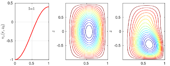
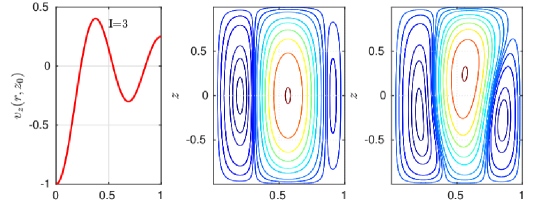
Figure 5: ($1^{st}~{}coulum$) Driver ion’s velocity profile at $z=z_{0}$ for radial sheared mode numbers $I=1~{}and~{}3$. Corresponding streamlines pattern for the dust fluid flows in $r-z$ crossection for ($2^{nd}~{}coulum$) $\mu=10^{-3}[U_{0}L_{r}]$, and ($3^{rd}~{}coulum$) $\mu=3\times 10^{-5}[U_{0}L_{r}]$ respectively.

The flow structures are analyzed for two important cases of kinematic viscosity, i.e., $\mu=10^{-3}[U_{0}L_{r}]$ for the linear regime and $\mu=10^{-5}[U_{0}L_{r}]$ for the nonlinear regime which corresponds to flow regimes Re$~{}\approx 0.001$ and Re$~{}\approx 50.0$ respectively. In these regimes, the dust fluid flows within the velocity range of $1-50~{}mm/sec$, while the dust acoustic speed $c_{ds}$ is found to be $12~{}cm/sec$ in the domain. As observed in the earlier analysis Laishram et al. (2015, 2014), the flow structure in the linear regime is characterized by a system of symmetric and elongated circulations (or streamlines that are aligned with the confining boundaries) as shown in Fig. 5 ($2^{nd}~{}coulum$). The alternating positive and negative shear in the external driving field in case of $I=~{}3$ leads to the formation of counter-rotation in addition to scales introduced by the confining boundary and stationary background fluid Laishram et al. (2015). However in the nonlinear regime, as shown in Fig. 5($3^{rd}~{}coulum$), the flow structure changes into an asymmetric and elongated circulation with a finite displacement of the center of circulation ${\bf(u(r_{0},z_{0})=0)}$. In the case of multiple vortices (in the $I=~{}3$ case), the circulation center shifts along with the driver. In many dusty plasma experiments Tsytovich et al. (2003); Kaur et al. (2015a), similar multiple dust vortices are observed to correlate with scales of the ion dragging interaction in background. Further, a remarkable property of the present analysis is that the geometry and the dimension of steady driven dust vortex structure in the linear regime are mainly asserted by the confining boundary whereas in the nonlinear regime, the structure is mostly controlled by the dynamical regime rather than the boundary. Such vortex dynamics and structural changes are observed in recent dusty plasma experiments. For example, S. Mitik et. al. Mitic et al. (2008b) observed dust vortex driven by neutral gas convection, and structural variation with change in pressure in the applied field. In another experiment, T. Hall et. al. Hall and Thomas (2016) observed the asymmetric response of dust clouds to a change in the relative strengths of the electrostatic and ion drag forces at varying pressure.

III.3 Flow structure dependence on the dynamical regime and domain aspect ratio.

The influence of various system parameters or dynamical regimes on vortex structure is further analyzed explicitly for the $I=1$ case (Fig. 5, $1^{st}~{}row$). For the driven-dissipative system, the steady state momentum equation can be written as

$$({\bf u}\cdot\nabla){\bf u}=-\frac{\nabla{P}}{\rho}-{\nabla{V}}+\mu\nabla^{2}{\bf u}-\xi({\bf u}-{\bf v_{s}})-\nu({\bf u}-{\bf w_{n}}).$$

Applying the condition for the center of circulation, i.e., ${\bf u(r_{0},z_{0})=0}$, the equation at ${(r_{0},z_{0})}$ reduces to

$$\frac{\nabla{P}}{\rho}+{\nabla{V}}-\mu\nabla^{2}{\bf u}=\xi{\bf v_{s}}+\nu{\bf w_{n}}.$$ (16)

Here, $P$ is the dynamic pressure of the incompressible flow which becomes a function of velocity ${\bf u}$, which again depends on $\mu$. V is the effective confining potential and the diffusion transport $\mu\nabla^{2}{\bf u}$ at the center point $(r_{0},z_{0})$ is negligibly small.

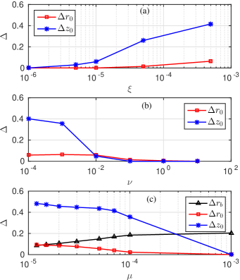
Figure 6: Shift of circulation center ($r_{0},z_{0}$) as function of (a) ion dragging co-efficient $\xi$, (b) neutral collision frequency $\nu$, and (c) kinematic viscosity $\mu$. The boundary layer thickness $\Delta r_{b}$ as function of $\mu$ is also plotted in (c).

Now, Fig. (6)(a) and (b) shows the radial and axial shifts of the center point $(r_{0},z_{0})$ with respect to $\xi$ and $\nu$ respectively. The radial shift $\Delta r_{0}$ is small in each case, while the axial shift $\Delta z_{0}$ with $\xi,~{}\nu$ is high in the higher Reynolds regime. However in the case of $\mu$ variation shown in Fig. (6)(c), the shift $\Delta z_{0}$ increases slowly in the higher Re regime. Further, the radial shift $\Delta r_{0}$ and the change in boundary layer thickness $\Delta r_{b}$ due to varying kinematic viscosity $\mu$ correlate with each other. The different variations in radial and axial shifts of the center of circulation $(r_{0},z_{0})$ with respect to system parameters suggest that the steady flow structure also depends on the aspect ratio ($L_{z}/L_{r}$) of the confined domain. This may be because in the nonlinear regime, $({\bf u}\cdot\nabla){\bf u}$ introduces new scale $L_{\|}\sim(u/u^{\prime})$ in addition to the diffusion scale ($L_{\perp}$). The analysis of nonlinear flow characteristics in a domain of unity aspect ratio ($L_{z}/L_{r}=1$)Laishram et al. (2017, 2018) shows that the shifting in both the $\Delta z_{0}$ and $\Delta r_{0}$ are relatively small and similar.

IV Summary and conclusions

A 2D hydrodynamical model is developed for the dynamics of a dust fluid embedded in a combination system of an unbounded sheared ion flow and a background stationary neutral fluid. The validity of the present numerical solution is verified by comparing the flow profiles produced by the previous analytical solution in the linear limitLaishram et al. (2015). Improving from the earlier analysisLaishram et al. (2014, 2015), this model has the freedom of choosing any form of the driving flows, confining boundaries, and arbitrary Reynolds number regimes. The vortex structure of the steady dust fluid in the poloidal cross-section is analyzed within the transition range of Reynolds number $0.001<Re\leq 50$ where the dust flow with speed ranges from $0.1~{}mm~{}to~{}3~{}cm$ while the dust acoustic speed is about $12~{}cm/sec$. It has been observed that the geometry and dimension of the steady dust vortex in the linear regime (Re$\leq 1$) is mainly determined by confining boundaries, whereas it is governed by the dynamics (or dynamical regime) rather than the boundaries in the nonlinear regime (Re$\gg 1$). Thus the steady dust flow structure in the linear regime is characterized by symmetric and elongated vortices with various scales mainly introduced by the driving fields and boundaries. However at Re$\gg 1$, the steady dust flow structure is no longer symmetric. Instead, a new asymmetric and elongated structure appears with scales mainly dependent on the driven-dissipation parameters such as $\xi$, $\nu$, and $\mu$ in addition to the aspect ratio of the confined domain.

It is concluded that steady driven and bounded dust flow in an unbounded streaming plasma can possess various flow structures in linear and nonlinear dynamic regimes depending on scales introduced by non-uniformity of the unbounded external driving field and the system parameters including aspect ratio and those of confining boundaries. The numerical model is generic and applicable for other driven-dissipative systems such as the microscopic biological system and the gigantic Jovian vortices. Further analysis on the nonlinear flow characteristics and its stability in various aspect ratios and arbitrary Re regimes will be reported in future publications.

References

- (1)
- Holzer et al. (2010) L. Holzer, J. Bammert, R. Rzehak, and W. Zimmermann, Phys. Rev. E 81, 041124 (2010), URL http://link.aps.org/doi/10.1103/PhysRevE.81.041124.
- Grossmann (2000) S. Grossmann, Rev. Mod. Phys. 72, 603 (2000), URL https://link.aps.org/doi/10.1103/RevModPhys.72.603.
- Laishram et al. (2015) M. Laishram, D. Sharma, and P. K. Kaw, Phys. Rev. E 91, 063110 (2015), URL http://link.aps.org/doi/10.1103/PhysRevE.91.063110.
- Laishram et al. (2014) M. Laishram, D. Sharma, and P. K. Kaw, Phys. Plasmas 21, 073703 (2014), URL http://dx.doi.org/10.1063/1.4887003.
- Lauga and Powers (2008) E. Lauga and T. R. Powers, Rep. Prog. Phys. 79 (2008).
- Wolgemuth (2008) C. W. Wolgemuth, Biophys. J. 95, 1564 (2008), ISSN 0006-3495, URL http://www.sciencedirect.com/science/article/pii/S0006349508701231.
- Pan et al. (2013) L. Pan, A. Morozov, C. Wagner, and P. E. Arratia, Phys. Rev. Lett. 110, 174502 (2013), URL http://link.aps.org/doi/10.1103/PhysRevLett.110.174502.
- Yager and H. (2006) E. T. H. K. Yager, Paul and B. H., Nature (London) 442, 412 (2006), URL http://dx.doi.org/10.1038/nature05064.
- Squires and Quake (2005) T. M. Squires and S. R. Quake, Rev. Mod. Phys. 77, 977 (2005), URL http://link.aps.org/doi/10.1103/RevModPhys.77.977.
- Stroock et al. (2002) A. D. Stroock, S. K. W. Dertinger, A. Ajdari, I. Mezić, H. A. Stone, and G. M. Whitesides, Science 295, 647 (2002), ISSN 0036-8075.
- Sommeria and L. (1988) M. S. D. S. Sommeria, Jöel and H. L., Nature (London) 331, 689 (1988), URL http://dx.doi.org/10.1038/331689a0.
- Choi et al. (2007) D. S. Choi, D. Banfield, P. Gierasch, and A. P. Showman, Icarus 188, 35 (2007), ISSN 0019-1035, URL http://www.sciencedirect.com/science/article/pii/S0019103506004179.
- Marcus (1990) P. S. Marcus, J. Fluid Mech. 215, 393–430 (1990).
- Nivedita (2017) L. P. P. I. Nivedita, Nivedita, Scientific Reports 7, 44072 (2017), URL http://dx.doi.org/10.1038/srep44072.
- Fortov et al. (2003) V. E. Fortov, O. S. Vaulina, O. F. Petrov, V. I. Molotkov, A. V. Chernyshev, A. M. Lipaev, G. Morfill, H. Thomas, H. Rotermell, S. A. Khrapak, et al., JETP 96, 704 (2003), ISSN 1090-6509, URL http://dx.doi.org/10.1134/1.1574544.
- Morfill et al. (1999) G. E. Morfill, H. M. Thomas, U. Konopka, H. Rothermel, M. Zuzic, A. Ivlev, and J. Goree, Phys. Rev. Lett. 83, 1598 (1999), URL http://link.aps.org/doi/10.1103/PhysRevLett.83.1598.
- Thomas et al. (1994) H. Thomas, G. E. Morfill, V. Demmel, J. Goree, B. Feuerbacher, and D. Möhlmann, Phys. Rev. Lett. 73, 652 (1994), URL http://link.aps.org/doi/10.1103/PhysRevLett.73.652.
- Kaur et al. (2015a) M. Kaur, S. Bose, P. K. Chattopadhyay, D. Sharma, J. Ghosh, Y. C. Saxena, and E. T. Jr., Phys. Plasmas 22, 093702 (2015a), URL http://dx.doi.org/10.1063/1.4929916.
- Kaur et al. (2015b) M. Kaur, S. Bose, P. K. Chattopadhyay, D. Sharma, J. Ghosh, and Y. C. Saxena, Phys. Plasmas 22, 033703 (2015b), URL http://dx.doi.org/10.1063/1.4916065.
- Klindworth et al. (2000) M. Klindworth, A. Melzer, A. Piel, and V. A. Schweigert, Phys. Rev. B 61, 8404 (2000), URL http://link.aps.org/doi/10.1103/PhysRevB.61.8404.
- Mitic et al. (2008a) S. Mitic, B. A. Klumov, U. Konopka, M. H. Thoma, and G. E. Morfill, Phys. Rev. Lett. 101, 125002 (2008a), URL http://link.aps.org/doi/10.1103/PhysRevLett.101.125002.
- Fink et al. (2013) M. A. Fink, S. K. Zhdanov, M. Schwabe, M. H. Thoma, H. Höfner, H. M. Thomas, and G. E. Morfill, Europhys.Lett. 102, 45001 (2013), URL http://stacks.iop.org/0295-5075/102/i=4/a=45001.
- Arp et al. (2005) O. Arp, D. Block, M. Klindworth, and A. Piel, Phys. Plasmas 12, 122102 (2005).
- Landau and Lifshitz (2013) L. Landau and E. Lifshitz, Fluid Mechanics, v. 6 (Elsevier Science, 2013), ISBN 9781483140506, URL https://books.google.co.in/books?id=CeBbAwAAQBAJ.
- Barnes et al. (1992) M. S. Barnes, J. H. Keller, J. C. Forster, J. A. O’Neill, and D. K. Coultas, Phys. Rev. Lett. 68, 313 (1992), URL http://link.aps.org/doi/10.1103/PhysRevLett.68.313.
- Khrapak et al. (2002) S. A. Khrapak, A. V. Ivlev, G. E. Morfill, and H. M. Thomas, Phys. Rev. E 66, 046414 (2002), URL http://link.aps.org/doi/10.1103/PhysRevE.66.046414.
- Ivlev et al. (2004) A. V. Ivlev, S. A. Khrapak, S. K. Zhdanov, G. E. Morfill, and G. Joyce, Phys. Rev. Lett. 92, 205007 (2004), URL http://link.aps.org/doi/10.1103/PhysRevLett.92.205007.
- Press (1992) W. H. Press, The Art of Scientific Computing (Cambridge University Press, 1992).
- Weinan and Liu (1996) E. Weinan and J.-G. Liu, J. Comput. Phys. 124, 368 (1996).
- Tsytovich et al. (2003) V. N. Tsytovich, G. Morfill, U. Konopka, and H. Thomas, New J. Phys. 5, 66 (2003), URL http://stacks.iop.org/1367-2630/5/i=1/a=366.
- Mitic et al. (2008b) S. Mitic, R. Sütterlin, A. V. I. H. Höfner, M. H. Thoma, S. Zhdanov, and G. E. Morfill, Phys. Rev. Lett. 101, 235001 (2008b), URL http://link.aps.org/doi/10.1103/PhysRevLett.101.235001.
- Hall and Thomas (2016) T. H. Hall and E. Thomas, IEEE Trans. Plasma Sci. 44, 463 (2016).
- Laishram et al. (2017) M. Laishram, D. Sharma, P. K. Chattopdhyay, and P. K. Kaw, Phys. Rev. E 95, 033204 (2017), URL https://link.aps.org/doi/10.1103/PhysRevE.95.033204.
- Laishram et al. (2018) M. Laishram, D. Sharma, P. K. Chattopdhyay, and P. K. Kaw, AIP Conference Proceedings 1925, 020028 (2018), URL https://aip.scitation.org/doi/abs/10.1063/1.5020416.