Input-output analysis of Mach 0.9 jet noise

Abstract

We examine amplifying behavior of small perturbations about Reynolds-averaged Navier-Stokes solutions (RANS) of a $M_{j}=0.9$ subsonic turbulent jet using input-output (I/O) analysis. Singular value decomposition (SVD) of the resolvent of the linearized Navier-Stokes (LNS) equations forms an orthonormal set of I/O mode pairs, sorted in descending order by the magnitude of the corresponding singular values. In this study we design a filter to restrict input forcings to be active only in regions where turbulent kinetic energy (TKE) of jet turbulence is high. For an output domain, we directly implement the Ffowcs Williams-Hawkings (FWH) method within I/O analysis framework to measure far-field sound of observers distributed along an arc. In this way we find that the resulting TKE-weighted input modes captures coherent structures in the near-field of turbulent jets. Optimal input modes correspond to wavepackets represented by asymmetric pseudo-Gaussian envelope functions at a given forcing frequency. These wavepackets remain similar in shape over a range of frequencies for $St>0.5$, and scale as $St^{-0.5}$. While the optimal mode is a wavepacket, sub-optimal modes represent decoherence of the optimal input mode. By projecting high-fidelity large eddy simulation (LES) data onto the basis of input modes, we find that input modes do indeed capture the acoustically relevant dynamics in the jet. The far-field acoustics predicted by the LES are recovered using only a few number of I/O modes.

I Introduction

Since Lighthill’s pioneering work lighthill1952 , researchers have devoted more than 60 years to identifying the aerodynamic sources of sound in turbulence. Lighthill’s acoustic analogy rearranges the exact Navier-Stokes equations into the form of an inhomogeneous wave equation. The nonlinearities of the Navier-Stokes equations are lumped into the forcing terms on the right hand side of this equation. Corresponding to the acoustic sources in turbulent flows, these terms arise from deterministic nonlinear dynamics, but they are often studied only in terms of their statistics curle1955 ; phillips1960 ; ffowcs1963 ; lilley1974 ; goldstein2003 . In this framework, the acoustic analogy relates the statistics of the acoustic sources to the statistics of the far-field sound. This suggests that the sources of sound in turbulence may be viewed as stochastic and fine-scale: a quasi-random collection of point sources. In the early 1960s, however, Mollo-Christensen observed highly-organized vortical flow features within seemingly chaotic turbulent flow in jets mollo1963 ; mollo1967 . His work inspired fellow researchers to model aerodynamic sound generation associated with turbulence in terms of spatio-temporally coherent flow structures, modulated by growing and decaying envelopes crow1971 ; michalke1970 ; michalke1972 ; mattingly1974 ; crighton1976 ; michalke1984 ; tam1984 ; suzuki2006 . In recent years it has been found that such organized structures, now more popularly known as wavepackets, are closely connected to instability waves in jets jordan2013 .

Experiments crow1971 ; fuchs1972 ; fuchs1972b ; seiner1974 ; armstrong1977 ; moore1977 ; suzuki2006 ; reba2010 ; cavalieri2012 and simulations freund2001 ; suzuki2006 ; reba2010 ; cavalieri2012 have confirmed the presence of wavepackets in the near-field of high-speed turbulent jets. For a given a base flow, wavepackets can be efficiently computed using reduced-order methods based on the parabolized stability equations (PSE) cheung2007 ; gudmundsson2011 ; rodriguez2013 ; sinha2014 ; jordan2013 , global mode analysis nichols2011 , and optimal forcing approaches schmid2001 ; garnaud2013 ; nichols2014 ; jeun2016 . In addition, several studies have developed theoretical models of wavepackets based on experimental and numerical data michalke1977 ; crighton1990 ; reba2010 ; cavalieri2012 ; baqui2015 ; serre2015 . The theoretical models use analytic envelope functions to modulate an underlying instability wave. Both the compactness and the asymmetry of the wavepacket envelope affect its acoustic efficiency and directivity serre2015 .

In contrast to the fine-scale view of acoustic sources, wavepackets represent large-scale, coherent sources of sound. Given these two different views of aerodynamic production of sound in jets, it is natural to suppose that both mechanisms (large-scale and fine-scale) may be active simultaneously in high-speed jets. In support of this, experimental measurements of far-field acoustic spectra of jets over a wide range of operating conditions seem to be well-represented by the superposition of two similarity spectra tam1996 . Acoustic radiation at small angles to the jet follows the Large-Scale Similarity (LSS) spectrum, whereas sideline noise radiation aligns with the Fine-Scale Similarity (FSS) spectrum. Compared to the LSS spectrum, the FSS spectrum tends to have lower peak levels, but is active over a broader range of frequencies. It is important to note, however, that the LSS/FSS spectra are constructed only from the statistics of the far-field acoustics, and thus are not directly connected to the near-field dynamics. Even within the statistical framework, however, refined statistical models of jet acoustic sources that account for decoherence and acoustic interference at high radiation angles reveal that both the LSS and FSS spectral shapes can be recovered from a single source mechanism karabasov2010 . Compared to the two-source model, this represents a significant reduction in complexity.

It has recently been shown, however, that a dynamical model based on stochastic similarity wavepackets can match experimental measurements of a Mach 0.9 over a large range of frequencies and observer angles papamoschou2011 . Compared to statistical models of jet noise, stochasticity enters into this model in just six places, yet further reducing the dimensionality and complexity of the acoustic source system. Moreover, the stochastic wavepacket model offers physical insight into the dynamical mechanisms responsible for sound production. On the other hand, while the stochastic similarity wavepacket model matches experimental measurements, the analysis starts on a surface in the near-field surrounding the jet, and so is not directly connected to the jet turbulence. The analysis assumes the near field of a jet can be modeled as a superposition of wavepackets appearing and disappearing intermittently in time and space. Furthermore, the model is based on a choice of the functional shape of these wavepackets, although wavepackets at different frequencies are related to one another by a similarity variable.

In the current paper, we address these issues by applying I/O analysis to connect far-field acoustics directly to the turbulence-containing regions of a Mach 0.9 jet. Our previous study showed that for supersonic jets, I/O analysis recovers the downstream peak jet noise radiation associated with the LSS spectrum, which PSE calculations also predict jeun2016 . Our analysis also showed that sideline noise can be recovered from a small number of sub-optimal I/O modes, not predicted by PSE-based methods. The fact that sideline noise can be generated by a small number of modes suggests that it is generated by large-scale flow features, rather than fine-scale flow features that the FSS spectrum assumes. This suggests that jet noise at all observer angles may be connected to large-scale flow features, and explains why the stochastic wavepacket model works as well as it does.

In the analysis presented below, we examine I/O analysis in the context of wavepacket models of jet noise. Our analysis depends crucially on a careful description of how forcing from turbulence drives a linear systems model of the jet dynamics, and of how acoustic outputs are measured. While our analysis is based on resolvents, our I/O formulation allows us to investigate only those dynamics in the jet that are connected to significant noise radiation. This distinguishes our analysis from other resolvent-based approaches schmid2001 ; garnaud2013 which focus upon modes that are energetically important in terms of the jet aerodynamics, but which may or may not radiate significant noise. This distinction is important, as it is well known that only a small fraction of the total fluctuation energy in a jet is radiated as sound dowling1983 ; jordan2013 .

Focusing in this way upon the acoustically dominant dynamics, the question of physical interpretation then remains: are the acoustically important dynamics organized into large-scale modes, or can they only be described by fine-scale fluctuations? We are specifically interested in quantifying the dimensionality (or rank) of the acoustically important dynamics. Can these dynamics be represented by a reduced-order model as the stochastic similarity wavepacket model suggests? In this paper, we address these questions by comparing the results of our I/O analysis to high-fidelity simulations to show that acoustic source dynamics are indeed low-rank. As a rigorous test, we focus upon a Mach 0.9 jets, including its sideline noise, which traditionally is a case that has posed the largest challenge for PSE-based methods. Moreover, we show that the low-rank acoustics source dynamics are organized into similarity wavepackets, even for sound emitted at large angles to the jet axis. This provides physical justification for the theoretical stochastic similarity wavepacket model of jet noise.

The rest of this paper is organized as follows. In Sec. II we define a base flow and governing equations. We also describe a hybrid input-output/Ffowcs Williams-Hawkings (I/O-FWH) method and its numerical parameters in the same section. In Sec. III we compare our I/O results to previous wavepacket models. We show that the optimal input modes obtained from I/O analysis are in fact self-similar over a range of frequencies. In addition to the optimal modes, the physical origin of sub-optimal modes is also discussed. In Sec. IV, we project high-fidelity large eddy simulation data onto a set of input modes. This provides further insight into the physical meaning of our input modes, and suggests that a particular type of jitter may be responsible for a significant portion of the sound production in subsonic jets. Our conclusions are discussed in Sec. V.

II Methodology

II.1 Base flow

We consider a Mach 0.9 isothermal, round, turbulent jet matching the conditions of the experiment used as a basis for the stochastic similarity wavepacket model papamoschou2011 . Isothermal Mach 0.9 jets have also been the subject of several other experimental and numerical investigations shur2005 ; cavalieri2011 ; cavalieri2011b ; bres2015 . Like supersonic jets, Mach 0.9 jets support instability waves and wavepackets that can be predicted by stability analysis based on either the PSE jordan2014 or the linearized Euler equations jeun2016 . In supersonic jets, these wavepackets are directly connected to the acoustic far-field through the mechanism of Mach wave radiation tam1995 . In subsonic jets, however, wavepackets are not as directly connected to the far-field. In particular, a subsonic wavepacket does not radiate sound at its associated peak wavenumber. In wavenumber space, acoustic radiation comes instead from the supersonic “tail” of the wavepacket jordan2013 . This depends on the modulation and asymmetry of the wavepacket envelope in physical space serre2015 . The result is that, in isolation, wavepackets seem to underpredict the sound generated by subsonic jets. This underprediction is partially rectified by introducing either “jitter” or a decoherence scale into the model. The stochastic similarity wavepacket model incorporates these effects through a randomized superposition of coherent wavepackets, which, by fitting, can closely reproduce experimentally measured far-field acoustic spectra. Applying I/O analysis, we found acoustic source terms may be linked to several sub-optimal modes in addition to the wavepacket jeun2016 . The sub-optimal modes were especially important for subsonic jets. For this reason, we focus upon a Mach 0.9 jet for the remainder of the paper. We will provide an interpretation of the physics behind optimal and sub-optimal acoustic sources predicted by I/O analysis and use this to explain the success of the stochastic similarity wavepacket model.

Figure 1 shows a Reynolds-averaged Navier-Stokes (RANS) solution of the jet computed using a modified $k-\varepsilon$ turbulence model for high-speed jets thies1996 as a base flow. The flow exhausts from a straight cylindrical nozzle with inner diameter $D=1$ and finite thickness $t=0.1D$. Along the wall, no-slip boundary conditions are employed, allowing boundary layers to grow as the flow travels downstream. The upstream boundary conditions are chosen to produce the desired jet exit velocity, pressure, and temperature at $x/D=0$. In terms of the jet diameter $D$, the jet Reynolds number $Re=\rho_{j}u_{j}D/\mu=2\times 10^{5}$, where $\mu$ is the constant dynamic viscosity across the full numerical domain. Here, $\rho_{j}$ and $u_{j}$ are respectively the density and the velocity at the nozzle exit. Throughout this paper, the geometry and properties of the jet flow are scaled by the jet diameter $D$ and properties measured at the nozzle exit denoted by subscripts $j$. While Fig. 1 visualizes only part of it, the actual numerical domain extends from $x/D=-10$ to $x/D=40$ and from $r/D=0$ to $r/D=25$ in the axial and radial directions, respectively.

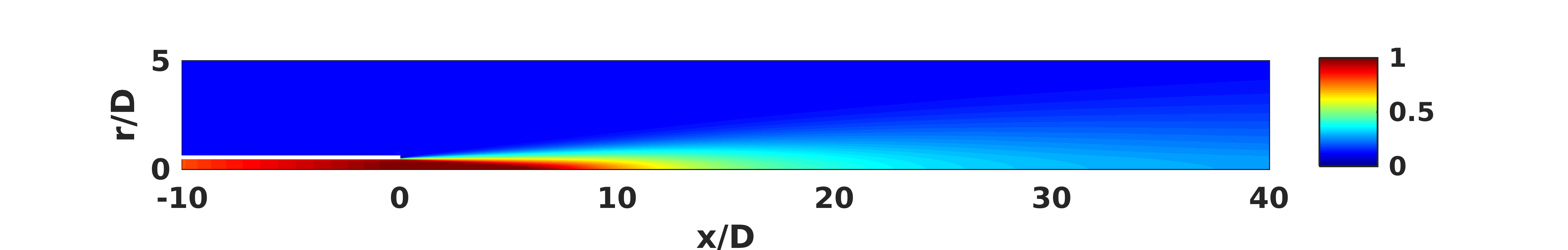
Figure 1: Contours of the real part of axial velocity of RANS solutions for the Mach 0.9 subsonic jet. The velocity contours are normalized by the velocity at the nozzle exit ($x/D=0$).

II.2 Linearized Navier-Stokes Equations

In this study the dynamics of high-speed turbulent jet is described by the fully compressible Navier-Stokes equations (NSE) for the system state $\bm{q}=\left[p;\,\bm{u}^{T};\,s\right]^{T}$, where $p$, $\bm{u}$ and $s$ are the fluid pressure, velocity, and entropy, respectively. Scaled with respect to the jet diameter and jet exit properties, the NSE are written in dimensionless form as:

$$\frac{\partial p}{\partial t}+\bm{u}\bm{\cdot}\bm{\nabla}p+\rho c^{2}\bm{\nabla}\bm{\cdot}\bm{u} =\frac{1}{Re}\left(\frac{1}{M_{j}^{2}Pr}\bm{\nabla}^{2}T+(\gamma-1)\Phi\right),$$ (1a)

$$\frac{\partial\bm{u}}{\partial t}+\frac{1}{\rho}\bm{\nabla}p+\bm{u}\bm{\cdot}\bm{\nabla}\bm{u} =\frac{1}{Re}\frac{1}{\rho}\bm{\nabla}\bm{\cdot}\bm{\tau},$$ (1b)

$$\frac{\partial s}{\partial t}+\bm{u}\bm{\cdot}\bm{\nabla}s =\frac{1}{Re}\frac{1}{\rho T}\left(\frac{1}{(\gamma-1)M_{j}^{2}Pr}\bm{\nabla}^{2}T+\Phi\right),$$ (1c)

and the equation of state for an ideal gas reads $\gamma M_{j}^{2}p=\rho T$, where $\gamma=1.4$ represents the constant ratio of specific heats. Here, the Prandtl number is defined as $Pr=c_{p}\mu/\lambda$, where $c_{p}$ is the specific heat at constant pressure and $\lambda$ is the thermal conductivity, which are assumed to be constant throughout the computational domain. Furthermore, $\Phi$ and $\tau$ denote the dissipation function and viscous stress function, respectively. In the last equation the entropy $s$ is set to be zero when $p=1$ and $T=1$, by defining $s=\ln(T)/\left((\gamma-1)M_{j}^{2}\right)-\ln(p)/\left(\gamma M_{j}^{2}\right)$ (see also nichols2009 ; nichols2011 ).

Using the standard Reynolds decomposition of the system state such as $\bm{q}=\overline{\bm{q}}+\bm{q}^{\prime}$, where $\overline{\bm{q}}$ represents the mean flow part and $\bm{q}^{\prime}$ is the fluctuating part, and keeping the first-order terms only, we write the linearized Navier-Stokes (LNS) equations as the governing equations for small fluctuations about which given base flows as:

$$\frac{\partial p^{\prime}}{\partial t}+\bm{\bar{u}}\bm{\cdot}\bm{\nabla}p^{\prime}+\bm{u^{\prime}}\bm{\cdot}\bm{\nabla}\bar{p}+\bar{\rho}\bar{c}^{2}\bm{\nabla}\bm{\cdot}\bm{u^{\prime}}+\gamma(\bm{\nabla}\bm{\cdot}\bm{\bar{u}})p^{\prime}=$$

$$\hskip 8.53581pt\frac{1}{Re}\left[\frac{1}{M_{j}^{2}Pr}\lambda\bm{\nabla}^{2}T^{\prime}+(\gamma-1)\big{(}\bm{\bar{\tau}}\bm{:}\bm{\nabla}\bm{u^{\prime}}+\bm{\tau^{\prime}}\bm{:}\bm{\nabla}\bm{\bar{u}}\big{)}\right],$$ (2a)

$$\frac{\partial\bm{u^{\prime}}}{\partial t}+\frac{1}{\bar{\rho}}\bm{\nabla}p^{\prime}+\frac{\rho^{\prime}}{\bar{\rho}}\bm{\nabla}\bar{p}+\bm{\bar{u}}\bm{\cdot}\bm{\nabla}\bm{u^{\prime}}+\bm{u^{\prime}}\bm{\cdot}\bm{\nabla}\bm{\bar{u}}=\frac{1}{Re}\frac{1}{\bar{\rho}}\left(\bm{\nabla}\bm{\cdot}\bm{\tau^{\prime}}-\frac{\rho^{\prime}}{\bar{\rho}}\bm{\nabla}\bm{\cdot}\bm{\bar{\tau}}\right),$$ (2b)

$$\frac{\partial s^{\prime}}{\partial t}+\bm{\bar{u}}\bm{\cdot}\bm{\nabla}s^{\prime}+\bm{u^{\prime}}\bm{\cdot}\bm{\nabla}\bar{s}=$$

$$\hskip 8.53581pt\frac{1}{Re}\frac{1}{\bar{\rho}\bar{T}}\bigg{[}\frac{1}{(\gamma-1)M_{j}^{2}Pr}\bigg{(}\lambda\bm{\nabla}^{2}T^{\prime}-\frac{p^{\prime}}{\bar{p}}\lambda\bm{\nabla}^{2}\bar{T}\bigg{)}+\bm{\bar{\tau}}\bm{:}\bm{\nabla}\bm{u^{\prime}}+\bm{\tau^{\prime}}\bm{:}\bm{\nabla}\bm{\bar{u}}-\frac{p^{\prime}}{\bar{p}}\bm{\bar{\tau}}\bm{:}\bm{\nabla}\bm{\bar{u}}\bigg{]}.$$ (2c)

In summary, the resulting linear system is written in matrix form as:

$$\frac{\partial\bm{q}}{\partial t}=A\bm{q},$$ (3)

where the linear operator $A$ corresponding to the governing equations is determined uniquely by a base flow.

II.3 Input-output analysis

The high-speed turbulent jets we consider in the present paper are stable in a global sense but are unstable to convective perturbations. Such systems behave as selective noise amplifiers of external perturbations and thus, are best studied by analyzing their sensitivity to external forcing. I/O analysis achieves this by adding an external forcing term $\bm{f}$ to the original linear system (3) as follows:

$$\dot{\bm{q}} =A\bm{q}+B\bm{f},$$ (4a)

$$\bm{y} =C\bm{q},$$ (4b)

where $\bm{y}$ represents output quantities, $B$ and $C$ are matrices determined depending on inputs and outputs of interests, respectively. For example, we specify $B$ to select forcings applied to the velocity equations near the jet turbulence while $C$ is chosen to specify noise in the region far way from sources. In this way our analysis investigates how input forcings map onto output quantities of interests. Specifying matrices $B$ and $C$ makes our analysis unique compared to other approaches which consider the entire system state to evaluate the gain.

To system (4), we apply the wavepacket ansatz as:

$$\bm{q}(x,r,\theta,t)=\hat{\bm{q}}(x,r)e^{\mathrm{i}(m\theta-\omega t)},$$ (5)

where $m$ is an azimuthal wavenumber and $\omega$ is a temporal frequency. By assuming similar harmonic forcing functions in this way, we find a transfer function $H$ from inputs to outputs that consists of a resolvent operator $R=(zI-A)^{-1}$ as:

$$y=C(zI-A)^{-1}Bf=Hf,$$ (6)

where $z=-\mathrm{i}\omega$. This is schematically described in Fig. 2. Singular value decomposition of the transfer function $H$ forms a set of pairs of input and output vectors, which respectively correspond to columns of matrices $V$ and $U$ in:

$$H=U\Sigma V^{*},$$ (7)

where the superscript ^∗ indicates the complex-conjugate transpose. Furthermore, the matrix $\Sigma$ is a diagonal matrix containing a set of singular values. Each singular value represents the amplitude gain from the corresponding input to output vectors that is defined as:

$$\sigma=\frac{\left\|\bm{y}\right\|}{\left\|\bm{f}\right\|},$$ (8)

where $\left\|\cdot\right\|$ denotes the $L^{2}$ norm.

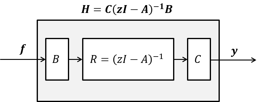
Figure 2: A schematic representation of the linear system in Eq. (4) using the transfer function $H$.

Finally, singular value decomposition of the transfer function may be computed through the eigen-decomposition of $H^{\dagger}H$:

$$H^{\dagger}H=B^{+}(z^{*}I-A^{\dagger})^{-1}C^{\dagger}C(zI-A)^{-1}B,\\$$ (9)

where $H^{\dagger}$ represents the adjoint of the transfer function, which maps outputs back onto inputs. Hence, the eigenvalues of $H^{\dagger}H$ are squares of the corresponding singular values of $H$. For more details, please refer to jeun2016 .

II.4 TKE-weighted input modes

In high-speed jets, the sources of sound are embedded in the jet turbulence. Specifically, the nonlinear terms driving our system (i.e., the Lighthill sources) are proportional to the fluctuating Reynolds stress tensor. To model this, we weight input forcings by the turbulent kinetic energy (TKE) as shown in Fig. 3, which is evaluated using the same RANS model used in computing the base flow.

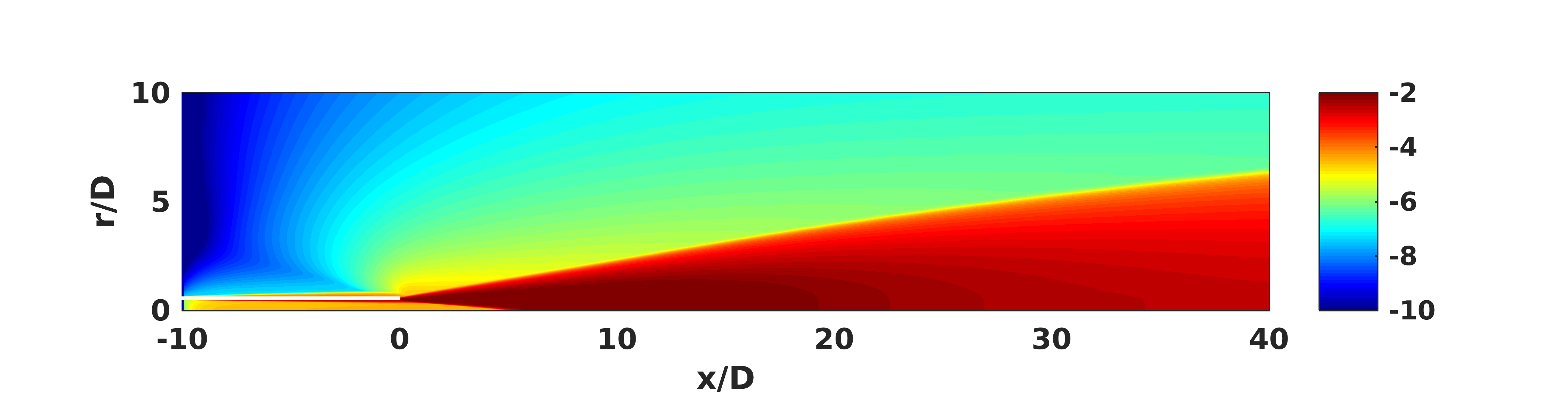
Figure 3: Contours of the TKE for the $M_{j}=0.9$ subsonic jet in logarithmic scale normalized by the square of the jet exit velocity.

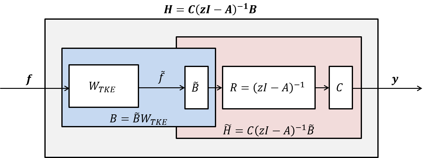
Figure 4: A schematic representation of the modified system with the TKE weighting matrix indicated by $W_{TKE}$.

A schematic description of the modified system with TKE-weighted input forcings is given in Fig. 4. Here, the TKE-weighting filter denoted by $W_{TKE}$ is applied to input forcings $\bm{f}$, yielding the TKE-weighted input forcings $\bm{\tilde{f}}$ written as:

$$\bm{\tilde{f}}=W_{TKE}\bm{f}.$$ (10)

The resolvent $R$ remains unchanged since it uniquely depends on the base flow. The matrix $C$ also remains the same as before. In this way the original, unweighted system in Eq. (4) becomes:

$$\dot{\bm{q}} =A\bm{q}+B\bm{f}=A\bm{q}+\tilde{B}\bm{\tilde{f}},$$ (11a)

$$\bm{y} =C\bm{q},$$ (11b)

where

$$\tilde{B}=BW_{TKE}^{-1}.$$ (12)

Because we are interested in output produced by the weighted inputs $\bm{\tilde{f}}$, we consider a new transfer function $\tilde{H}$ corresponding to the red box in Fig. 4. This new transfer function $\tilde{H}$ is related to the transfer function $H$ in the original, unweighted system such that:

$$\tilde{H}=C(zI-A)^{-1}\tilde{B}=HW_{TKE}^{-1}.$$ (13)

Consequently, by substituting Eqs. (10) and (13) into the Arnoldi iteration of $H^{\dagger}H$:

$$\bm{f}_{new}=H^{\dagger}H\bm{f}=W_{TKE}\tilde{H}^{\dagger}\tilde{H}W_{tke}\bm{f}=W_{TKE}\tilde{H}^{\dagger}\tilde{H}\bm{\tilde{f}},$$ (14)

we obtain that:

$$\bm{\tilde{f}}_{new}=W_{TKE}^{2}\tilde{H}^{\dagger}\tilde{H}\bm{\tilde{f}}.$$ (15)

Note that without weighting by the TKE, i.e., when $W_{TKE}=I$, the system returns to the original, unweighted system described in Sec. II.3.

II.5 Hybrid I/O-FWH solver

In this study, we focus upon the jet dynamics that generate the largest amount of far-field sound. These dynamics may be different from those having the greatest energy. The outputs $\bm{y}$ of interest are the far-field pressure of observers located along an arc. Extending the numerical domain to the far-field, however, requires a huge amount of computational resources. Instead, a projection method such as the FWH method may be employed to compute the far-field pressure from the near-field flow data. Since we consider a linearized system, the source terms to the FWH equations are also linear. We therefore treat them explicitly so that we can write the FWH formulation as a linear operator inside the matrix $C$. In this way the adjoint of the matrix $C$ takes far-field pressure fluctuations and maps these back onto state vectors on the FWH surface, which are then injected into the system. Further details about the derivation of the FWH solver and two test cases are provided in the appendix.

Since the FWH solver is linearized, a projection surface should be placed in purely acoustic region that is sufficiently far from the jet turbulence. To ensure that we are in the linear regime in LES, we select a straight cylinder with radius $r/D=6$ whose axis lies along the jet centerline as a projection surface. Using this, we measure the far-field pressure of probes uniformly distributed along an arc at a distance of $100$ jet diameters from the nozzle exit. The observer angles range from $\phi=10^{\circ}$ to $\phi=150^{\circ}$ with an increment of $\Delta\phi=1^{\circ}$, where the polar angle $\phi$ is measured from the downstream jet axis. These angles are chosen by considering the extent of the FWH surface and sponge layers to prevent outgoing waves from reflecting back. The choice of arc then naturally excludes regions outside of the sponge layers, avoiding spurious modes. A schematic of this hybrid I/O-FWH analysis is given in Fig. 5.

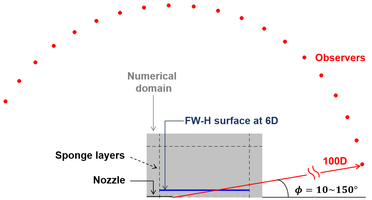
Figure 5: A schematic representation of the hybrid I/O-FWH analysis method. A straight cylindrical FWH projection surface is located at $x/D=6$, denoted by a blue straight line. Red dots indicate observers distributed uniformly along an arc in far-field from $\phi=10^{\circ}$ to $\phi=150^{\circ}$.

II.6 Numerical methods

We use fourth-order centered finite difference scheme to discretize the LNS on a stretched mesh. Since the non-dissipative nature of the centered finite difference scheme may introduce unphysical waves for high wavenumbers, a scale-selective fourth-order numerical filter is applied to suppress only the highest wavenumbers supported by the mesh. Furthermore, non-reflecting boundary conditions are satisfied by employing numerical sponge layers khalighi2010 ; mani2012 at the upstream ($x/D=-5$), downstream ($x/D=35$), and lateral boundaries ($r/D=20$).

The convergence of I/O analysis was tested in an earlier study jeun2016 for various grid resolutions. As a trade-off between the computational cost and the accuracy of the solutions, we choose to use a mesh with $801$ and $288$ grid points in the axial and radial directions, respectively. Whereas the grids are distributed uniformly in the axial direction, they are clustered in the radial direction along the nozzle lipline to resolve the boundary layer and thin shear layer formed near the nozzle lip.

The eigen-decomposition of $\tilde{H}^{\dagger}\tilde{H}$ is performed efficiently using the implicitly restarted Arnoldi method (IRAM) implemented by the software package ARPACK lehoucq1998 . An inverse matrix of the resolvent operator is computed by the parallel SuperLU package li2003 . The adjoints are evaluated using the continuous adjoint approach, which derives the equations adjoint to the LNS first and discretizes them later to estimate the matrix $A^{\dagger}$. In this way we obtain one-sided differences consistent with continuous derivatives near to nozzle walls. Since $\tilde{H}^{\dagger}\tilde{H}$ is Hermitian, the resulting input modes are orthonormal to each other, and the Arnoldi method converges quickly.

III Results

III.1 Input-output modes

Applying the hybrid I/O-FWH methodology, we obtain a spectrum of singular values representing gains between inputs and outputs, as discussed in Sec. II.4. Figure 6 shows the first 50 singular values, ordered by amplification factor, for the Mach 0.9 jet at a forcing frequency of $St=0.59$. For the purposes of this paper, which focuses upon the physical meaning of the results of I/O analysis, it is sufficient to consider axisymmetric disturbances only ($m=0$). Our I/O formulation can handle higher azimuthal wavenumbers, however, which become important especially to describe noise radiation in the sideline direction jeun2018 . The first 29 singular values show a relatively slow decrease in amplification factor, which means that the first 29 I/O modes produce approximately the same amount of far-field noise per unit energy of forcing. This is consistent with previous results for subsonic jets, where sub-optimal I/O modes were found to produce nearly the same amplification as the optimal modes. This is in contrast, however, to supersonic jets where the optimal mode becomes dominant jeun2016 .

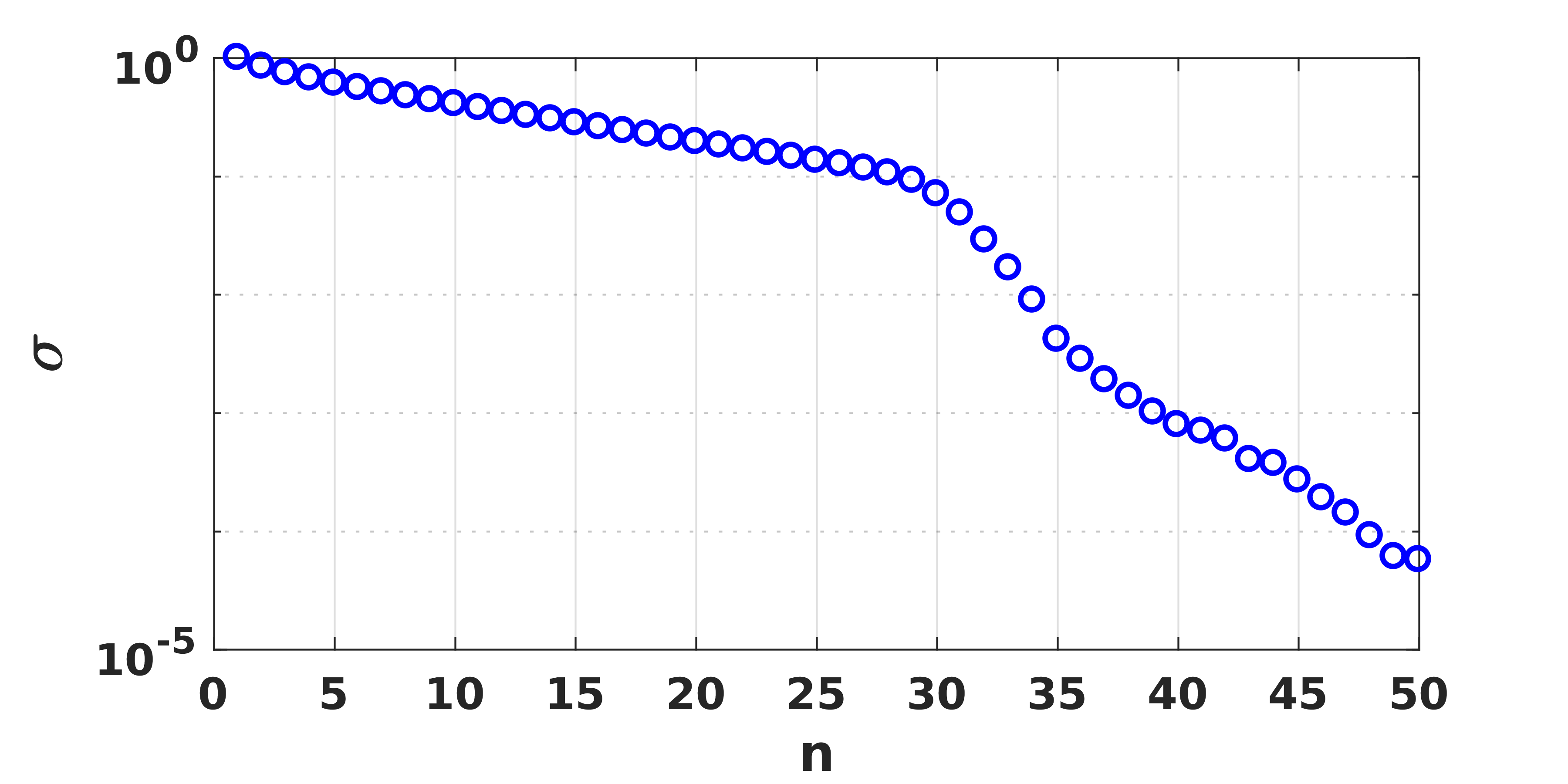
Figure 6: Singular values as a function of the mode number for the Mach 0.9 subsonic jet at forcing frequency $St=0.59$.

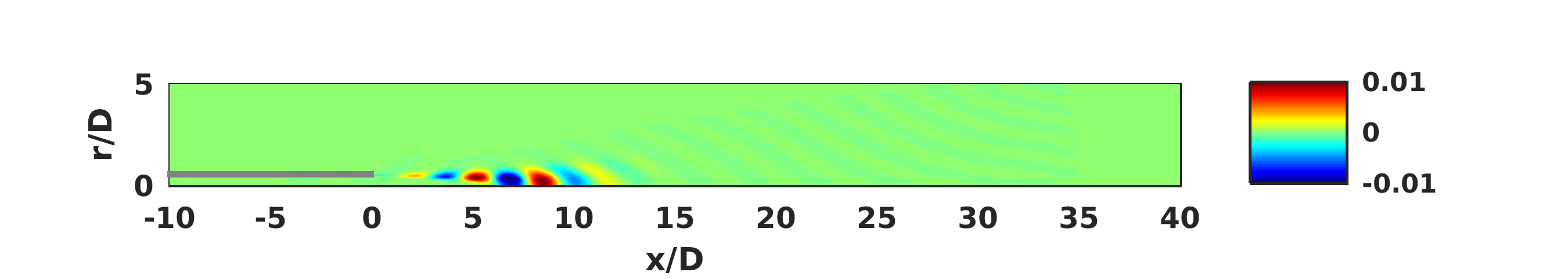
(a) $n=1$

(b) $n=2$

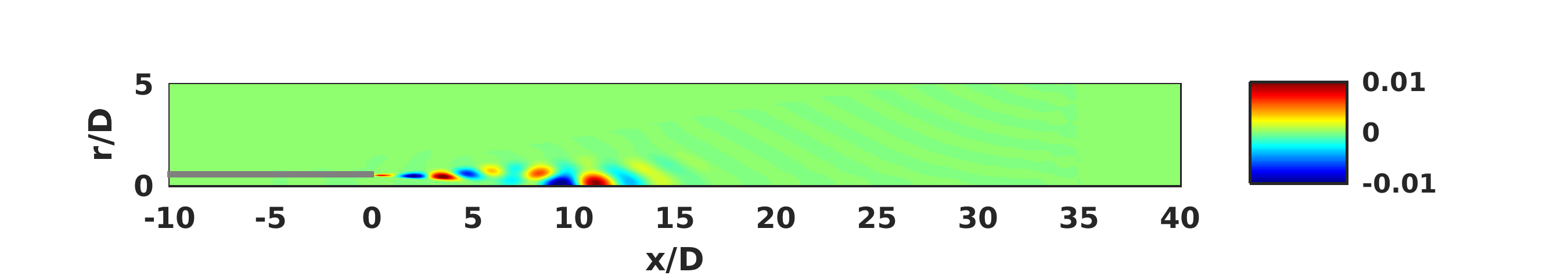
(c) $n=3$

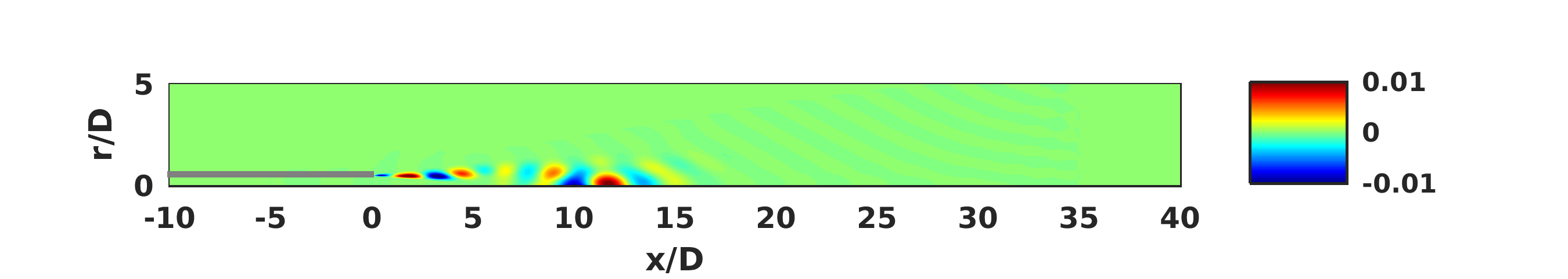
(d) $n=4$

Figure 7: The first four input modes of the Mach 0.9 jet for forcing frequency $St=0.59$. Contours visualizes the real part of the normalized axial velocity forcing.

Along with the gains, the singular value decomposition also produces orthogonal sets of corresponding input and output modes. Figure 7 shows the first four input modes corresponding to the four largest singular values shown in Fig. 6. In Fig. 7, the gray rectangle represents the nozzle wall, which ends at $x/D=0$. Contours showing the real part of the axial velocity forcing reveal the input modes to have significant structure. The optimal input mode ($n=1$), in particular, is clearly a wavepacket. At this frequency, the wavepacket is centered close to the end of the potential core of the jet, and extends several diameters upstream along the jet shear layers as well as downstream along the jet centerline. To characterize the physics of this wavepacket source, we consider the (complex) amplitude of the optimal input mode along the nozzle lipine ($r/D=0.5$). The blue solid line in Fig. 8 represents the absolute magnitude of the x-component of the input forcing for the optimal mode. Along this slice, we find a wavepacket that peaks around the end of the potential core (at $x/D=6$). Although the effect is subtle, this wavepacket grows slightly faster along its upstream edge than it decays downstream. Such asymmetric wavepackets have been observed in experiments and simulations and have been modeled theoretically by a variety of different functions michalke1977 ; crighton1990 ; reba2010 ; cavalieri2012 ; serre2015 ; baqui2015 . One of the most popular functional forms is the following asymmetric pseudo-Gaussian:

$$u_{x}(x)=\begin{cases}exp\left[-\left(\frac{x-b_{1}}{c_{1}}\right)^{p_{1}}\right],&\text{if x $\leq b_{1}$},\\ exp\left[-\left(\frac{x-b_{1}}{c_{2}}\right)^{p_{2}}\right],&\text{if x $\geq b_{1}$},\\ \end{cases}$$ (16)

where $b_{1}$ locates the peak of the wavepacket envelop, $c_{1}$ and $c_{2}$ respectively determine widths of the amplifying and decaying parts, and $p_{1}$ and $p_{2}$ represent the exponents, respectively. Applying a nonlinear least squares fitting algorithm, we find that $b_{1}=5.9375D,c_{1}=4.0599D,p_{1}=2.2545,c_{2}=4.5584D$, and $p_{2}=2.2517$ produce a pseudo-Gaussian curve that almost exactly matches our wavepacket. The fact that $p_{1}>p_{2}$ means that the wavepacket amplifies faster than it decays. This asymmetry is also indicated by $c_{1}<c_{2}$. Also, because both $p_{1}$ and $p_{2}$ are approximately equal to two, the shape of our wavepacket is nearly (but not quite) Gaussian. The shape of the wavepacket, and in particular its asymmetry, are important factors determining its efficiency at generating acoustic radiation serre2015 .

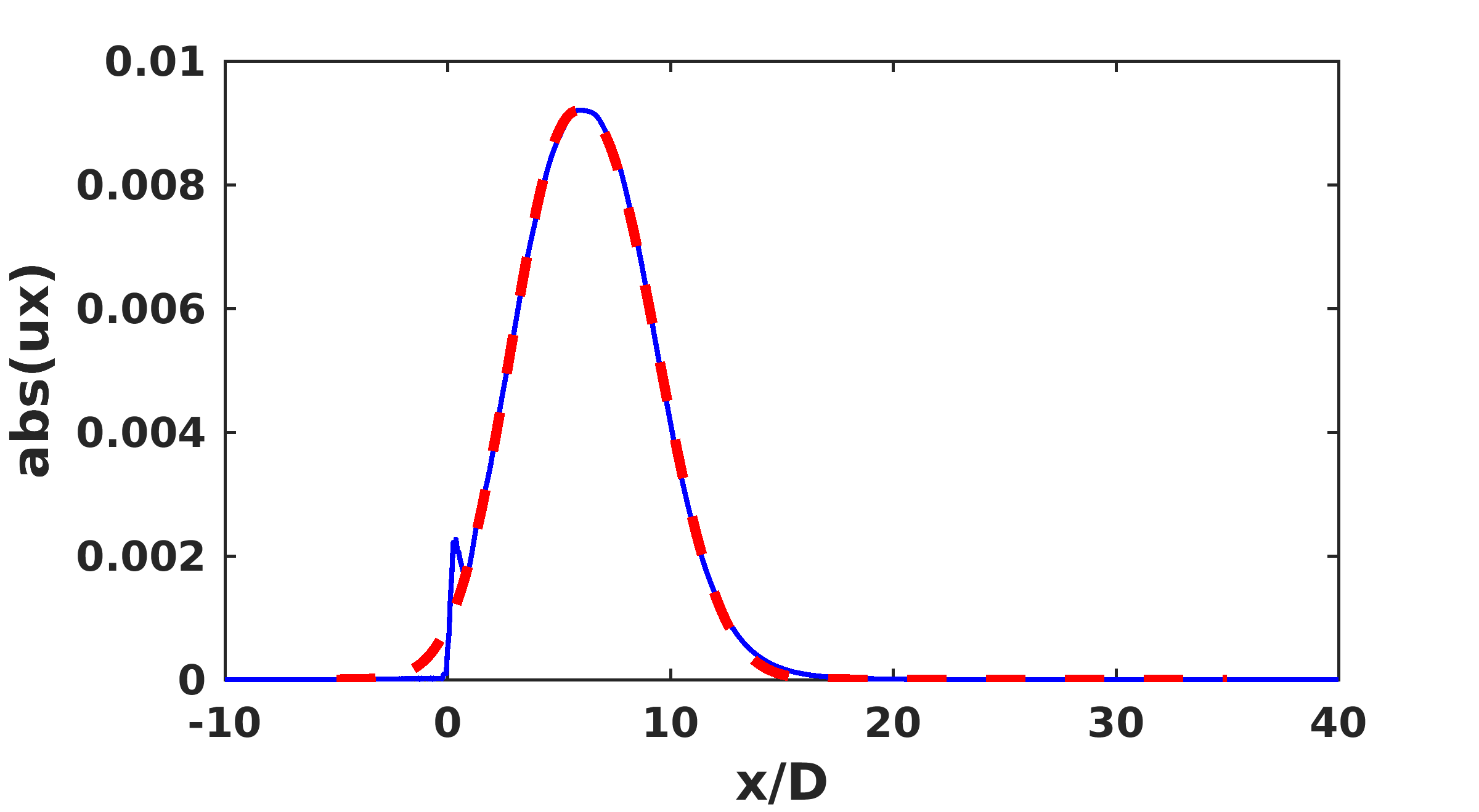
Figure 8: The lipline wavepacket measured at $r/D=0.5$ (blue solid line) modeled by an asymmetric pseudo Gaussian wavepacket (red dashed line) for the optimal mode of the $M_{j}=0.9$ subsonic jet at forcing frequency $St=0.59$.

While the leading input mode represents the optimal way to force a jet to make noise, Figs. 7(b)-(d) show sub-optimal input modes ($n=2,3,4$), which produce nearly the same amount noise as the optimal mode. They are active along upstream and downstream edges of the wavepacket associated with the optimal mode. As the mode number increases, the sub-optimal input modes progressively reach further upstream and downstream. To understand the pattern that they follow, it is helpful to to examine the sound fields they produce.

While the output domain is restricted to an arc at a distance of 100 jet diameters away from the nozzle exit, we can still obtain near-field sound associated with input modes by examining the system state after application of the resolvent operator, but before application of the output matrix $C$. We call these states “unrestricted” output modes. These modes extend over $-5<x/D<35$ in the axial direction and over $0<r/D<20$ in the radial direction, respectively. The output matrix $C$ later projects them to an arc in the far-field. As shown in Fig. 9, unrestricted outputs resulting from these inputs follows a similar pattern. Black dashed lines in this figure represent the upstream, downstream, and lateral sponge layers. The pattern is now clear: the optimal mode radiates a beam of acoustic radiation directed toward the peak jet noise angle for this frequency. Each sub-optimal output mode is active along the edges of the preceding mode. This creates two beams of acoustic radiation in the first sub-optimal mode, three in the second, and so on.

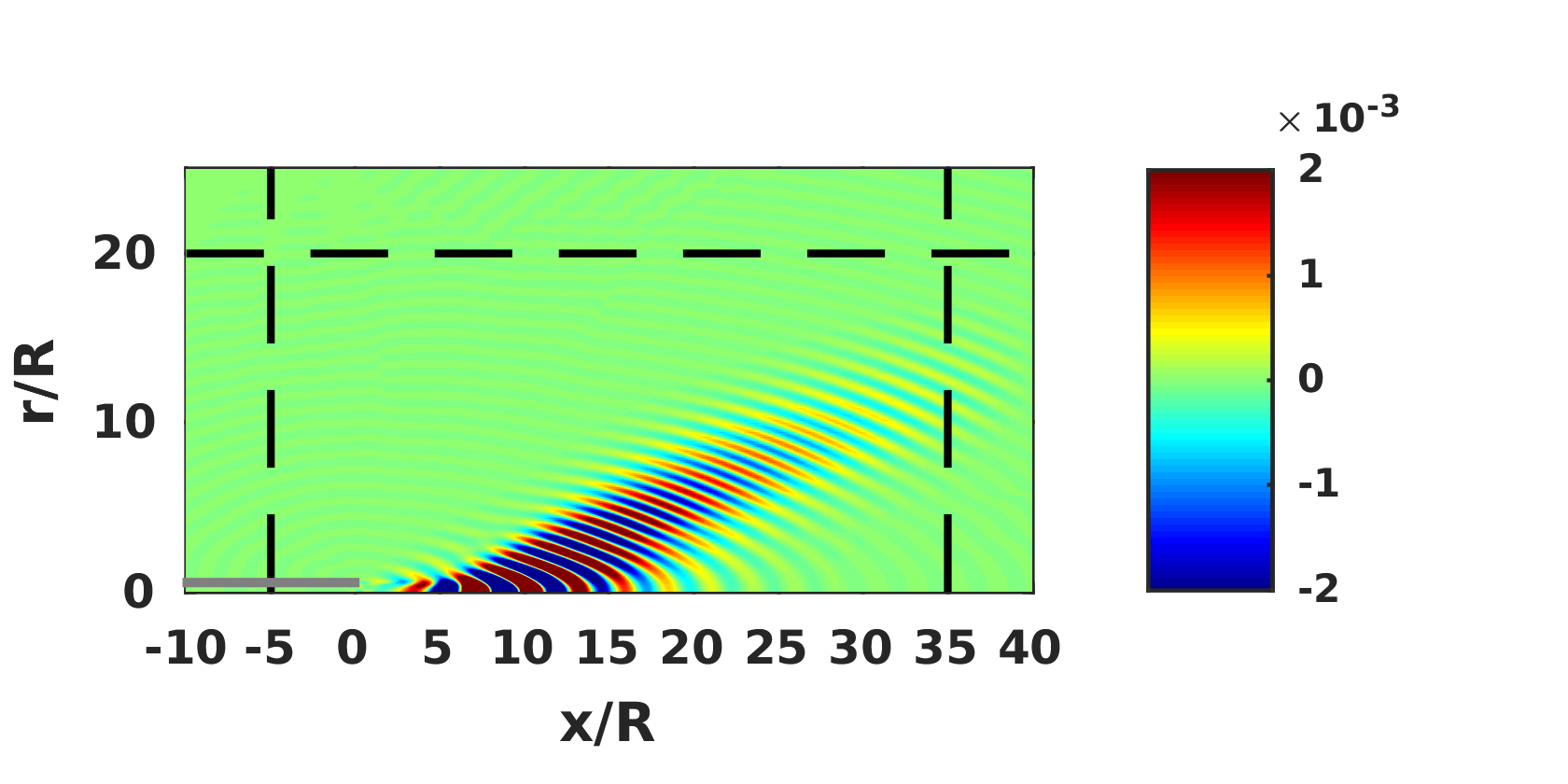
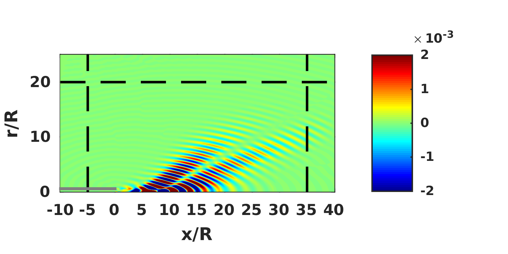
(a) $n=1$	(b) $n=2$
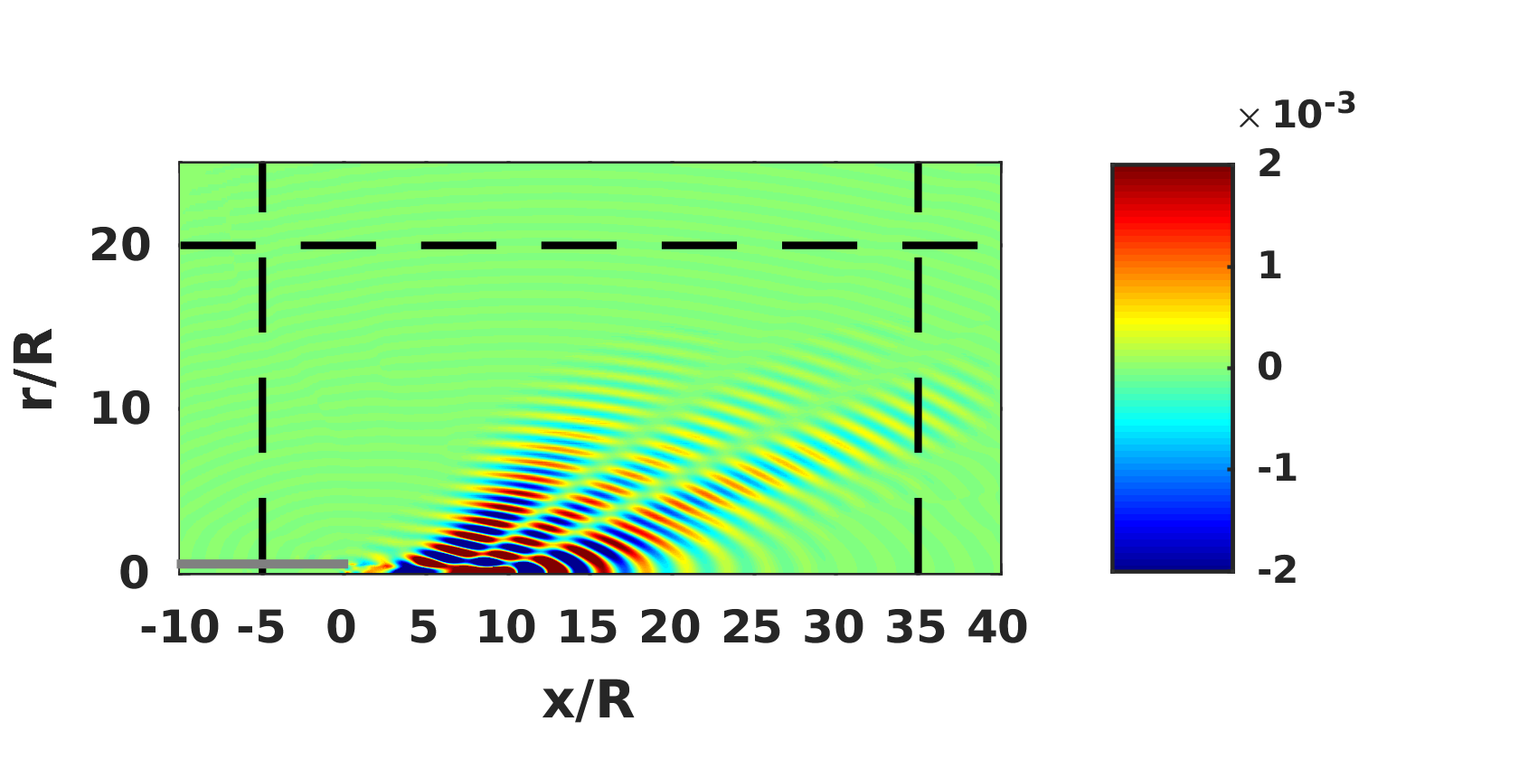
(c) $n=3$	(d) $n=4$

Figure 9: The first four unrestricted output modes of the Mach 0.9 subsonic jet at forcing frequency $St=0.59$. Contours of the real part of normalized output pressure fluctuations are shown.

III.2 Similarity wavepackets

III.2.1 Optimal mode

Although the lipline wavepacket associated with optimal input mode is well-described by a simple asymmetric function at one frequency, we repeat the modeling procedure over a range of frequencies. Motivated by the self-similarity of turbulent jets, we investigate whether similar asymmetric pseudo-Gaussian wavepacket functions can describe our input modes over different frequencies. Other wavepacket modeling approaches also have yielded self-similar asymmetric bell-shaped wavepackets over a range of frequencies papamoschou2010 ; papamoschou2011 . Naturally, the next task would be to construct a universal wavepacket model, which can be widely used for a range of frequencies, using minimum degrees of parameters; such as the first moment (mean or centroid of a wavepacket in the axial direction) $\mu_{1}$ and the standard deviation $SD$, which are respectively defined as:

$$\mu_{1}=\frac{\int{xu_{x}(x)dx}}{\int{u_{x}(x)dx}}$$ (17)

and

$$SD=\sqrt{\frac{\int{\left(x-\mu_{1}\right)^{2}u_{x}(x)dx}}{\int{u_{x}(x)dx}}}.$$ (18)

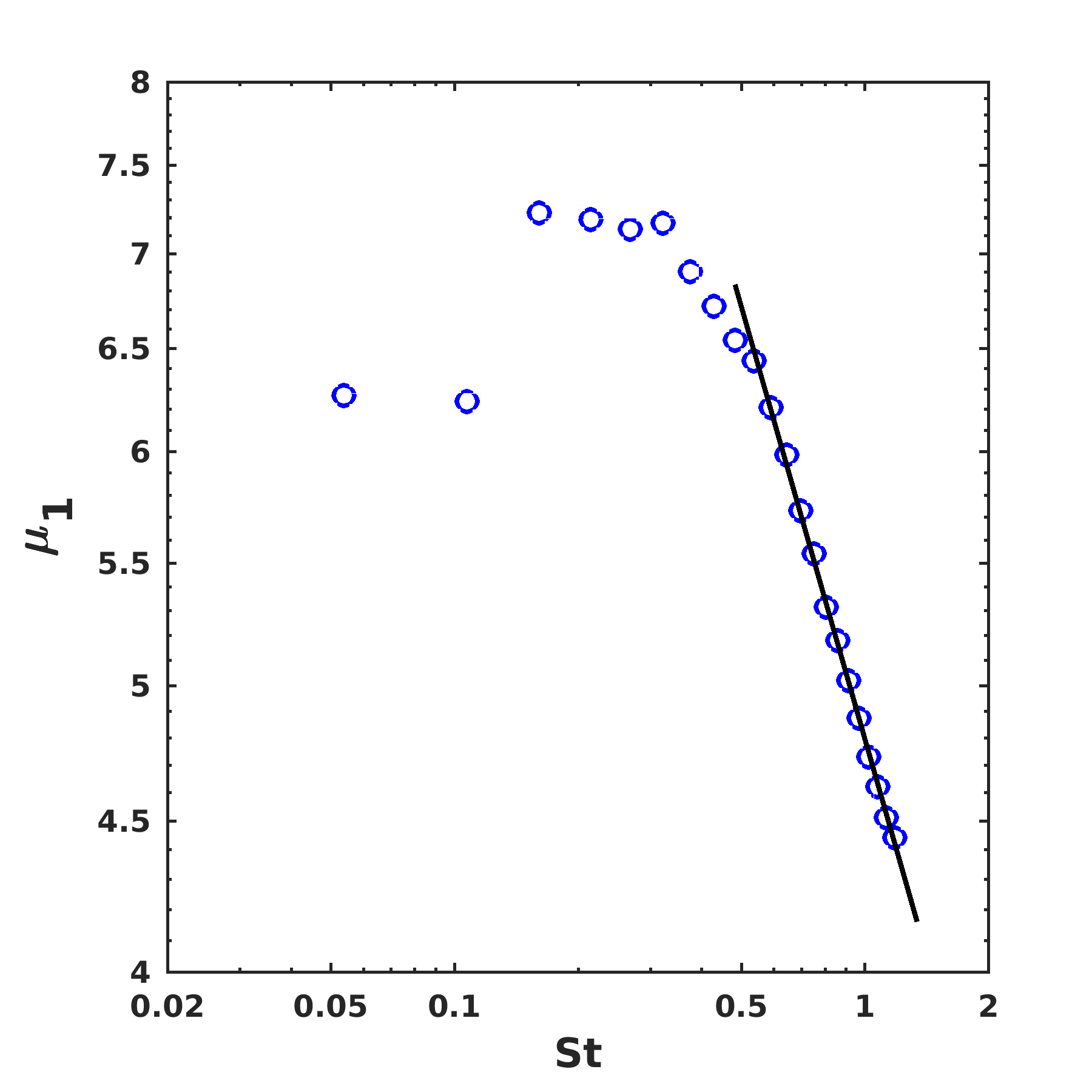
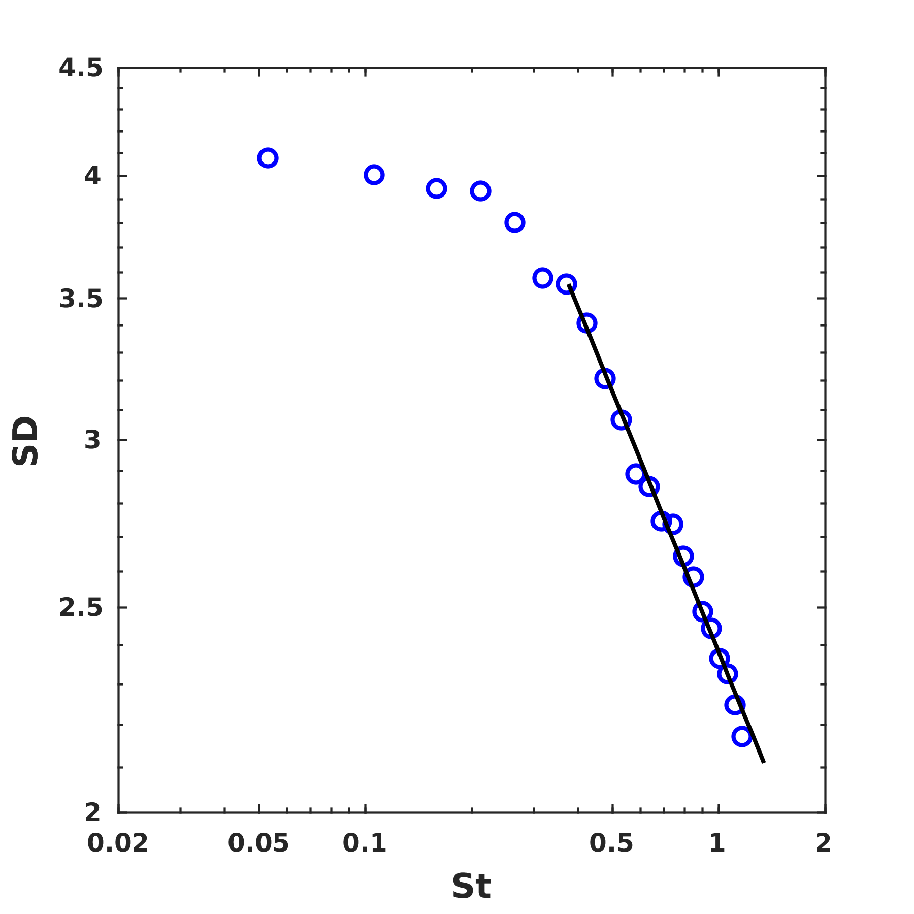
(a)	(b)

Figure 10: Model parameters as a function of frequencies for the lipline wavepacket: (a) the mean decays and (b) the standard deviation.

Figure 10 shows these quantities as a function of frequency. For sufficiently high frequencies, both the mean and standard deviation show a power-law dependence. As presented in Fig. 10(a) the mean location of the lipline wavepacket $\mu_{1}$ shifts upstream as forcing frequency increases. Excluding few low frequency cases, $\mu_{1}$ varies as $St^{-0.4858}$. Similarly, the standard deviation given in Fig. 10(b) follows the power-law form, though it decays slightly less rapidly than the mean as $St^{-0.4094}$. We observe such similarities for cases over $St>0.5$, and this agrees the result of theoretical approach by Papamoschou papamoschou2011 who reported the self-similarity of turbulent jets for $St>0.55$.

Furthermore, we compute the skewness of wavepackets for each frequency defined by:

$$SK=E\left[\frac{\left(x-\mu_{1}\right)^{3}}{SD^{3}}\right]$$ (19)

where $E$ means the expected value, $SD$ denotes the standard deviation, and $\mu_{1}$ represents the centroid of a wavepacket in the axial direction, respectively. Using this, Fig. 11 indicates positively skewed wavepackets for almost all frequencies as expected from long decaying tails. For frequencies $St>0.5$ wavepackets becomes more skewed as frequency increases, but overall, the variations of skewness remain small, suggesting similarity wavepackets in frequency.

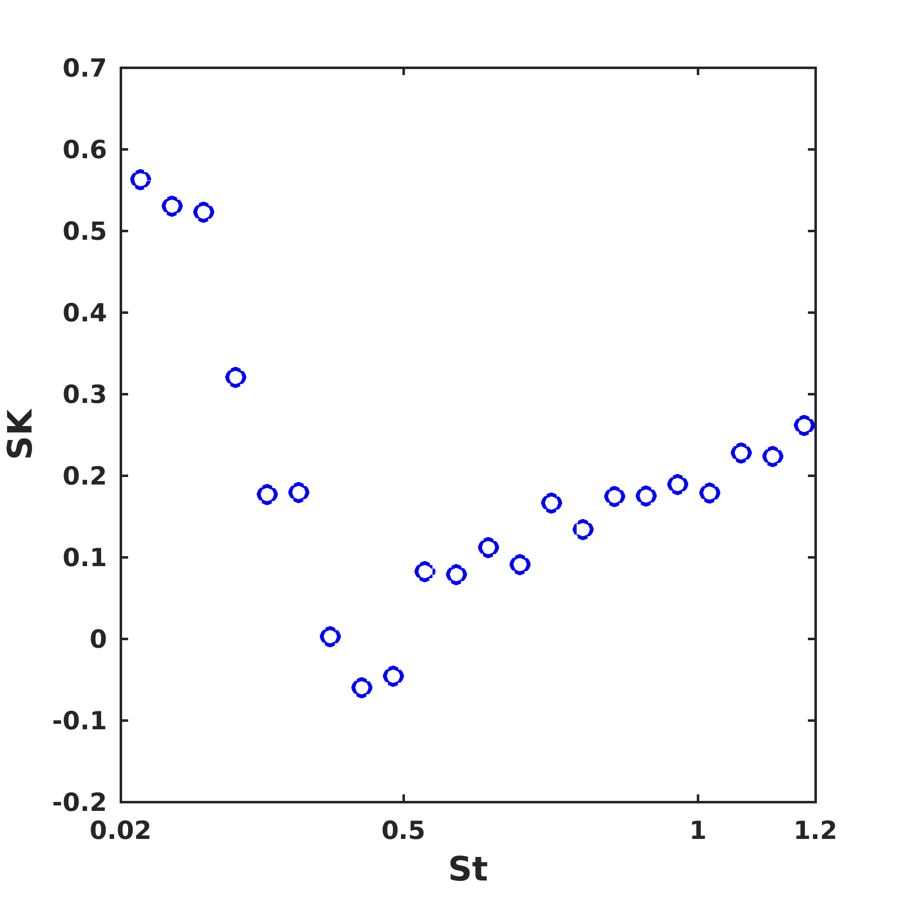
Figure 11: Skewness of the lipline wavepacket as a function of forcing frequency.

Finally, we construct wavepacket models, which are functions of a new variable $\eta$ transformed by the mean source location $\mu_{1}$ and scaled by the standard deviation $SD$ such as:

$$\eta=\frac{x-\mu_{1}}{SD}.$$ (20)

Here, instead of using two parameters $c_{1}$ and $c_{2}$ that control the widths of two parts of wavepackets separately, the standard deviation is chosen as a single unified parameter to describe the shape of wavepackets. Figure 12 shows the collapse of wavepacket envelopes taken over a range of frequencies between $St=0.5$ and $St=1.2$.

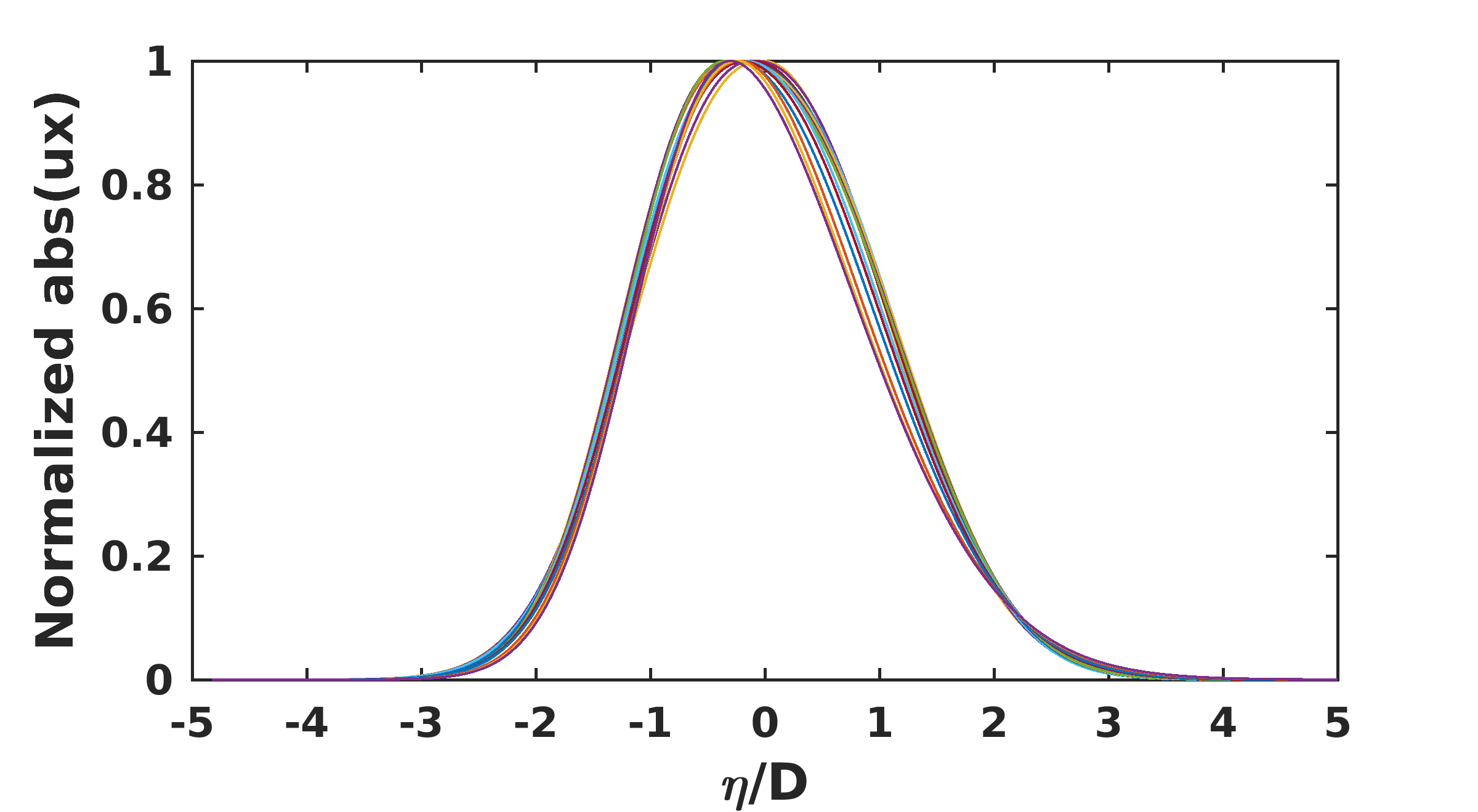
Figure 12: Collapse of scaled lipline wavepackets obtained for frequencies $0.5<St<1.2$, suggesting simple similarity wavepacket models based on the similarity variable $\eta$.

III.2.2 Sub-optimal modes

Sub-optimal modes appear to be composed of multiple wavepackets (see Fig. 7). The envelopes of these component wavepackets are similar in shape to that associated with the optimal mode. Because each sub-optimal mode conatins multiple wavepackets, modeling them is more complicated. Moreover, as the frequency changes, a group of wavepackets moves upstream and sometimes merges into the wavepacket in a boundary layer developed along the nozzle wall. It thus requires a great care to track the same type of wavepackets and model them as similarity wavepackets in frequency.

In Fig. 13 we model wavepackets taken along the jet lipline ($r/D=0.5$) for the first sub-optimal mode ($n=2$) by asymmetric pseudo-Gaussian functions. In contrast to the optimal mode, the first sub-optimal mode captures two wavepackets downstream of the nozzle exit ($x/D=0$). They, however, bear a similar shape to that captured by the optimal mode, and are approximated using the same type of asymmetric pseudo-Gaussian function given in Eq. (16). Here, the blue solid line represents the input-mode-captured wavepacket, while the red and green dashed lines denote modeled wavepackets.

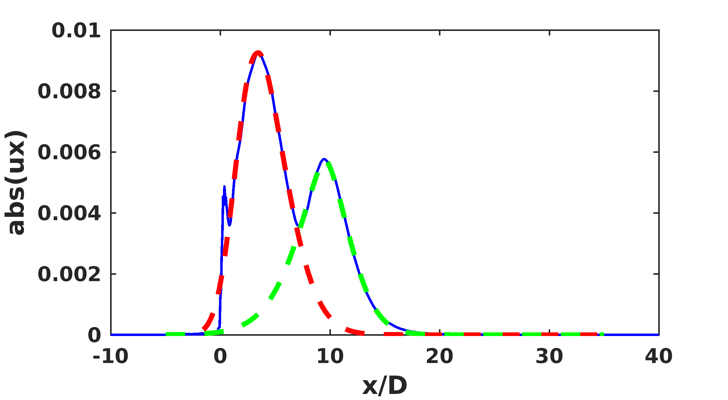
Figure 13: Wavepackets taken along the lipline for the first sub-optimal mode ($n=2$) at $St=0.59$ modeled using asymmetric pseudo-Gaussian functions. W1: red dashed line and W2: green dashed line, counted from the upstream.

Fig. 14 shows wavepackets taken along the inner lipline for mode number $n=3$ (the next sub-optimal mode). We observe three wavepackets, denoted by $W1$, $W2$, and $W3$, measured from the upstream. Each wavepacket is positively skewed and bell-shaped as in other cases. We therefore expect that a similarity wavepacket model could be constructed, even for this case.

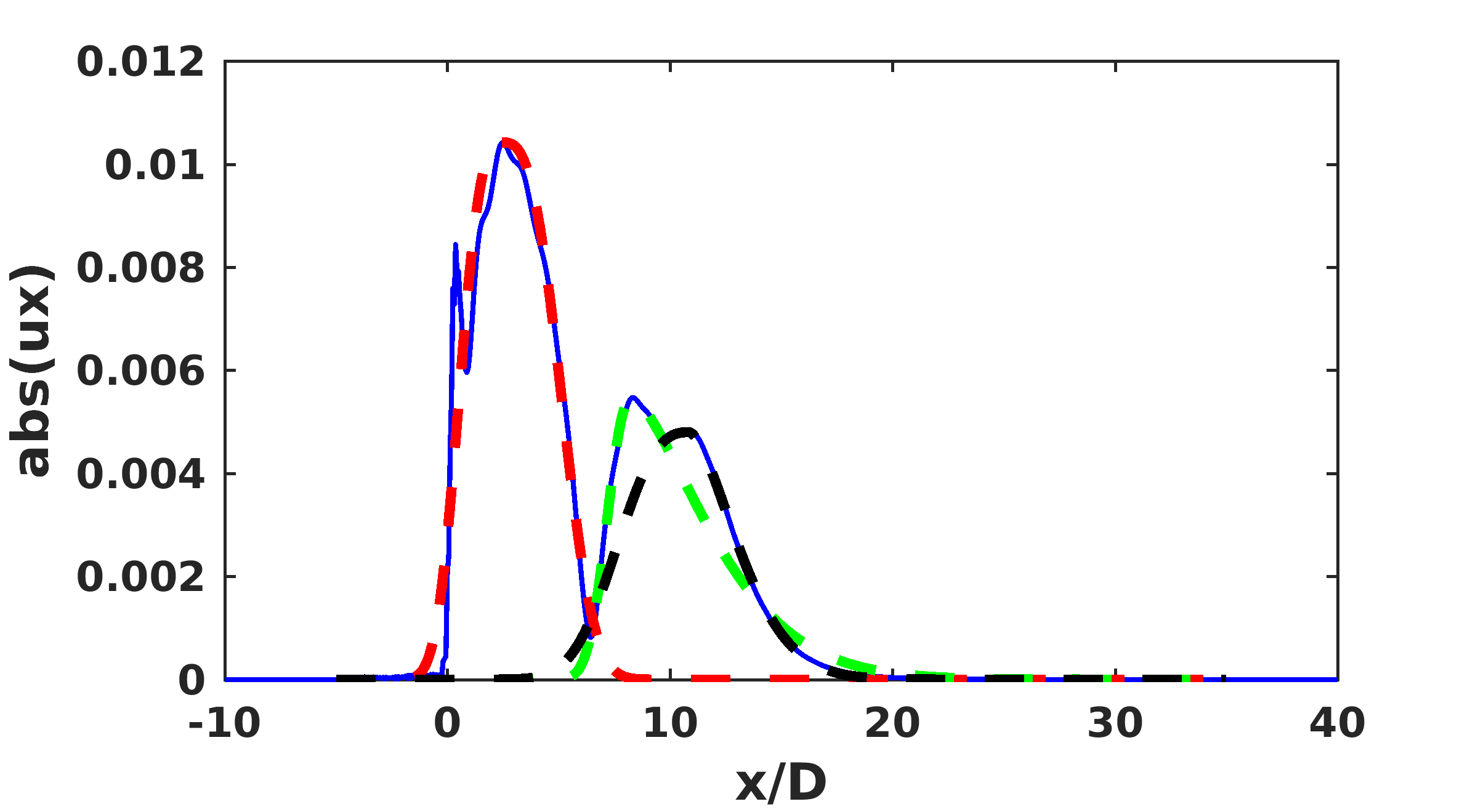
Figure 14: Wavepackets taken along the lipline for the second sub-optimal mode (blue solid line) at $St=0.59$ modeled using asymmetric pseudo-Gaussian functions. W1: red dashed line, W2: green dashed line, and W3: black dashed line, counted from the upstream.

The pattern shown in Figs. 12 through 14 is approximately the same that obtained by taking a sequence (of magnitudes) of axial derivatives of the optimal wavepacket envelope. Of course, the input modes are two-dimensional, so their inter-relationship may be more complicated than this. Still, the sub-optimal modes appear to be associated with dynamics in the regions where the amplitude of the preceding mode in the sequence is undergoing the most change (i.e., where its gradient is greatest). In the next section, we discuss physical mechanisms that could lead to sources that can align with such a pattern, thereby creating noise.

III.3 Physical origin of the sub-optimal modes

In previous sections, we found that the optimal input mode clearly reveals a wavepacket whose envelope corresponds to an asymmetric pseudo-Gaussian function. Moreover, we observed that the sub-optimal input mode captures structures that follow upstream and downstream edges of the optimal wavepacket. As shown in Figs. 13 and 14, the sub-optimal mode shows increasingly many humps as the mode number increases. The humps in each sub-optimal mode appear at locations where the largest differences would occur, if the wavepackets in the preceding mode were perturbed slightly in their axial position. This type of uncertainty in a wavepacket’s axial position is known as “jitter” cavalieri2011 ; jordan2013 ; jordan2014 . Jitter arises from the fact that high-speed jets are susceptible to variations at very low frequency, much lower than the frequencies associated with wavepackets. On the timescales of the wavepacket, this very low frequency variation appears to correspond to changes in the baseflow. The wavepacket responds to slow variations in the base flow by changing its position (and perhaps, shape). While axial jitter of the optimal wavepacket leads to a double-humped shape corresponding to the first sub-optimal mode, axial jitter of the first sub-optimal mode produces a shape with four humps. As shown in Fig. 14, the second sub-optimal mode has three humps.

Alternatively, we consider axial decoherence cavalieri2014 ; baqui2015 as another possible mechanism by which acoustic sources embedded in the jet turbulence may align with the pattern of sub-optimal modes that we find. Entire wavepackets are almost never visible in instantaneous snapshots of the near-field turbulent jets. Instead, one observes “pieces” of wavepackets that persist over a maybe only a few diameters before losing coherence. Inside these windows of coherence, fluctuations grow or decay in accordance to the overall wavepacket envelope. While the growth and decay of disturbances are governed by dynamics, wavepackets have a statistical nature as turbulence drives instability waves into and out of coherence. An entire wavepacket, therefore, should be thought of as the tendancy of the baseflow to make disturbances grow or decay in accordance with instability physics. Because these physics do not change in time for a given baseflow, a wavepacket is also constant and is determined by dynamics.

To model decoherence, we perturb the optimal wavepacket by small random forcing, and extract short, stochastic windows of it, positioned between $-5\leq x/D\leq 15$. The constant window width $w$ is chosen to be as large as the coherence length-scales of the axial velocities such that $w=2D$. Outside of a given window, we zero all other fluctuations. We repeat this process to build a stack of different realizations, visiting a different part of the wavepacket each time and reproducing the effect of its axial decoherence. Singular value decomposition applied to this collection yields its dominant dynamical features. As expected, the first singular vector recovers the original wavepacket (not shown). The right-hand column of Fig. 15 shows the first and second singular vectors obtained from the decomposition. While there are differences, they reproduce the corresponding sub-optimal modes fairly well. In particular, the 3rd singular vector contains three humps just like the second sub-optimal mode. This therefore conclude that axial decoherence is a physical mechanism by which acoustic sources in the jet align well with input modes predicted by I/O analysis.

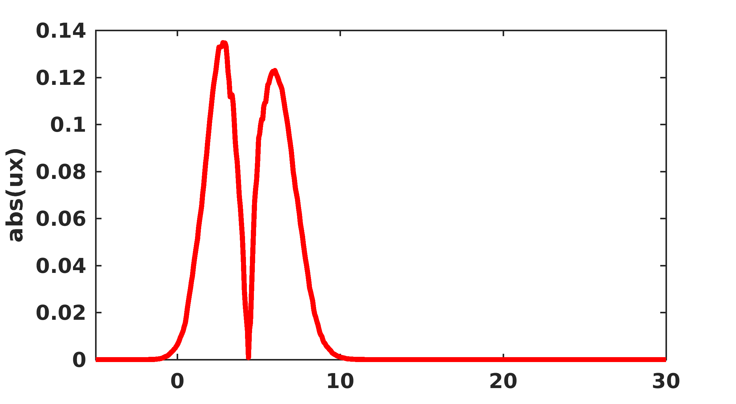
(a) $n=2$	(b) $n=2$
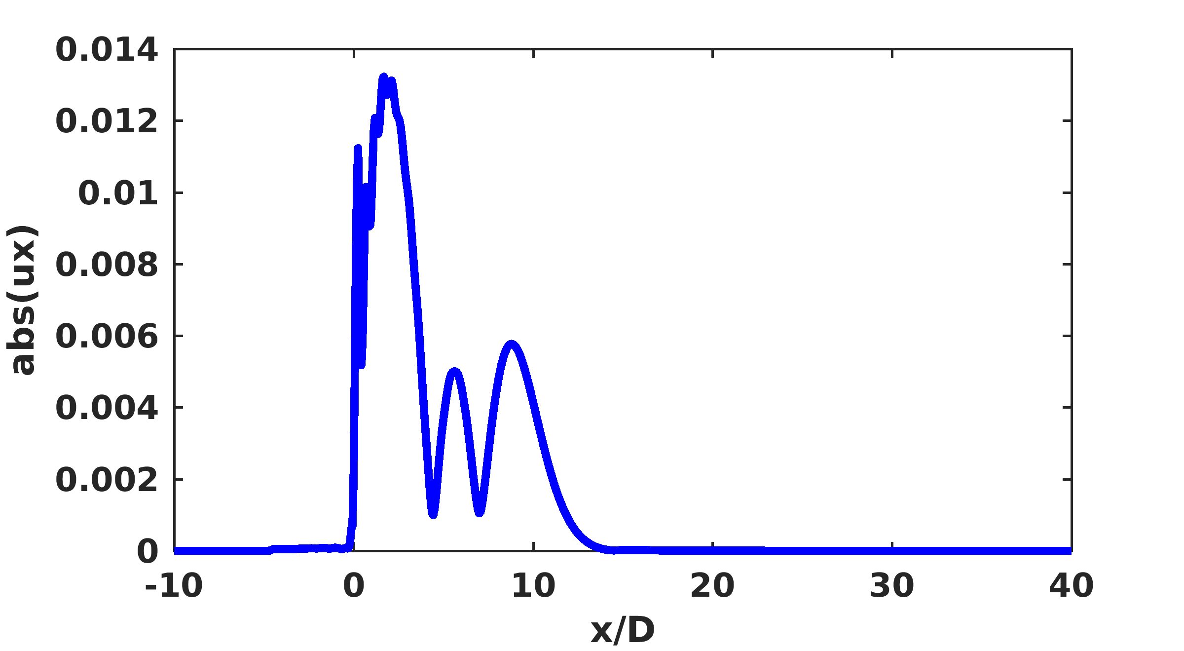
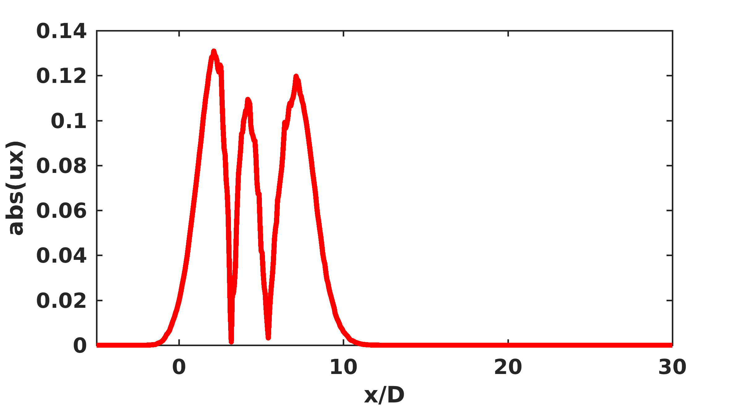
(c) $n=3$	(d) $n=3$

Figure 15: By taking singular value decomposition of the matrix whose columns consists of a series of axial snapshots of the optimal wavepacket, the left singular vectors (b,d) qualitatively reproduce the actual input modes (a,c) for $St=1.18$.

We should note that unlike the connection between input and output modes, there is not necessarily a causal relationship between axial decoherence modes and input modes. If it occurs, jitter may also project a significant portion of the sources onto the input modes. From our analysis, it seems that axial decoherence aligns even better with the input modes, and thus is an efficient mechanism of noise production.

IV Discussion

In the previous section, we saw that input forcing in the form of a wavepacket is the optimal way to generate far-field sound in a Mach 0.9 jet, according to I/O analysis. The wavepacket envelopes identified using our methodology agree well with theoretical models developed from experimental observations. Furthermore, we found that these wavepackets exhibit self-similarity over a broad range of frequencies. As the frequency increases, the peak of the corresponding wavepacket moves further upstream along the jet shear layers, closer to the nozzle. As the wavepacket moves closer to the nozzle, its axial extent diminishes, preserving similarity. This explains the success of a stochastic similarity wavepacket model papamoschou2011 at predicting experimental far-field acoustic spectra over a broad range of frequencies and observer angles.

While these results already paint a compelling picture of the physics of jet noise generation based on wavepackets, we further test them in this section by applying them to data obtained from a high-fidelity large eddy simulation (LES) of a Mach 0.9 jet. This provides additional insight about the meaning of the I/O modes, and ultimately about the mechanisms at play in the generation of sound in high-speed turbulent jets.

IV.1 Large eddy simulation

We perform large eddy simulation of a Mach 0.9 isothermal round jet using a finite volume method on an unstructured mesh. Our computational domain extends 10 nozzle diameters upstream of the nozzle exit and 50 diameters downstream. A numerical sponge layer, however, begins at 30 diameters downstream of the nozzle exit. This minimizes unphysical acoustic reflections at the outflow boundary. The radial extent of the domain is 25 nozzle diameters. To match the results based on RANS in the first part of the paper, we consider a straight cylindrical nozzle. We simulate the entire flow inside of the nozzle, starting at 10 diameters upstream of the nozzle exit. In Fig. 16, contours of temperature on a cross section through a snapshot taken from the LES show how the jet emerges from the straight nozzle and develops downstream. This figure also shows that while the temperature of the potential core matches the ambient temperature, the boundary layer in the nozzle and emerging shear layers heat slightly due to viscous dissipation. The Reynolds number of the jet based on nozzle diameter is $Re_{D}=u_{j}D/\nu=2\times 10^{5}$, which matches that of the RANS calculations. The unstructured mesh used for the results reported here incorporated 62 million cells, clustered in the turbulence-containing regions. The nozzle lip was resolved by approximately 800 cells in azimuthal direction. We repeated the LES on several different meshes to ensure that the reported results are grid independent. To account for turbulent motions on scales smaller than the grid resolution, we apply the Vreman sub-grid scale model.

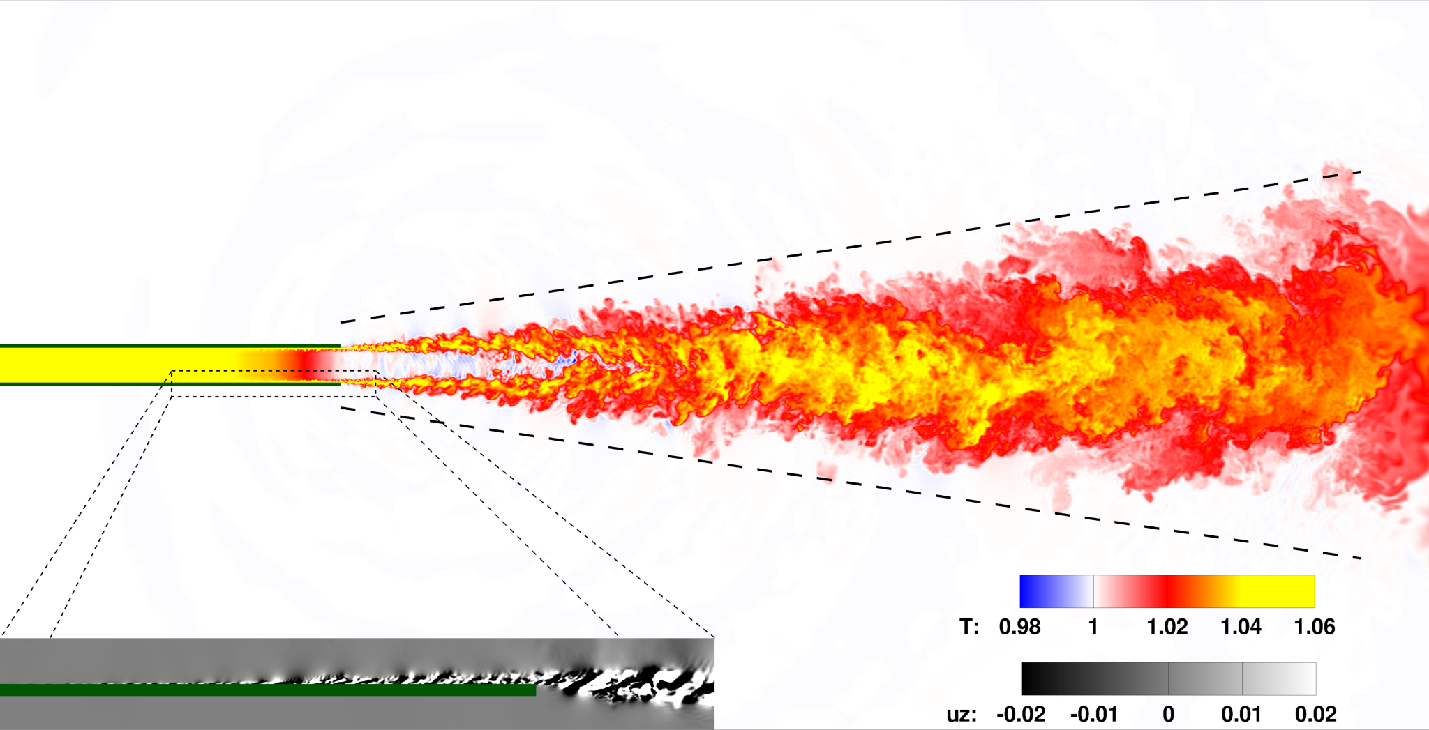
Figure 16: Contours of temperature and azimuthal velocity on a cross section through a snapshot taken from the LES of the Mach 0.9 turbulent jet.

The state of the boundary layer (laminar vs. turbulent) as it emerges from the nozzle can have a significant effect on the far-field sound produced by the jet zaman2012 ; bres2012 . To simulate realistic nozzle interior surface roughness levels, we trip the boundary layer by introducing low-level white noise in a zone around 7.5 diameters upstream of the nozzle exit. Several diameters downstream from this position, the boundary layers along the nozzle interior become turbulent before exiting the nozzle (see Fig. 16, inset).

To compute far-field sound, we collect acoustic information on a conical surface surrounding the jet, and project it to the far-field by solving the FWH equation lockard2000 ; lockard2005 ; bres2012 . The sloped dashed lines in Fig. 16 indicate the position of the conical surface relative to the jet. It is far enough from the jet for the flow to be essentially irrotational, but is close enough to remain in a zone of relatively fine resolution so that it captures acoustic waves with frequencies up to $St\approx 5$. Consistent with the FWH projection scheme used in the I/O analysis, the FWH surface is open on both ends. Comparing to results obtained using closed FWH surfaces (not shown), we find that the absence of end caps has little effect in this case, except at very low angles to the jet axis (less than $10^{\circ}$ or greater than $170^{\circ}$). This lack of effect is most likely due to the length of our FWH surface – it extends $30D$ downstream of the jet axis, well past the important acoustic source containing regions ($0<x/D<15$).

Once our simulation reaches a statistically stationary state, we run it for an additional time of $T=414D/c_{\infty}$, recording samples along the FWH surface at time intervals of $\Delta t=0.05D/c_{\infty}$ resulting in 8280 time samples total. In terms of the jet Strouhal number $St=fD/u_{j}$, this captures frequencies in the range $0.0027<St<11.11$, although the LES mesh resolution begins to affect frequecies at the high end of this range. Because the turbulent jet is a chaotic system, the convergence of the very lowest frequencies should not be trusted. Instead we apply a series of 25 Hann windows of length $82.8D/c_{\infty}$ to the data, overlapping with each other by 83.3%, and average the results (Welch’s method welch1967 ). Figure 17 shows far-field pressure spectra obtained using this method for observers located $50D$ away from the nozzle exit, at both $\phi=30^{\circ}$ and $90^{\circ}$ to the downstream jet axis for frequencies in the range $0.05<St<2$. The shape and levels of the spectra show excellent agreement with both experimental measurements bogey2007 and previous computations bres2015 . This demonstrates that our simulation produces realistic far-field noise.

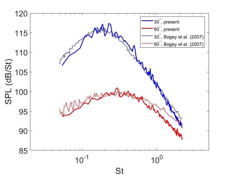
Figure 17: Far-field pressure spectra for observers located $50D$ away from the nozzle exit.

Figure 18 shows far-field sound spectra at $100D$ from the jet exit, and overall sound pressure levels as a function of polar angle at this same distance. Comparing Fig. 18(a) to Fig. 17, we see that the levels decrease at distances farther from the jet as expected. The shape of the spectra also change slightly. This is a consequence of the acoustic sources being extended over an axial distance in the jet. $50D$ is perhaps not so much larger than the $15D$ extent of the acoustic sources. To study the directivity of non-compact sources, it is important to project their sound farther away. We have chosen $100D$ to be relatively far away from the jet, but to remain within the realm of possible experimental measurement.

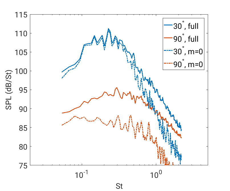
(a)

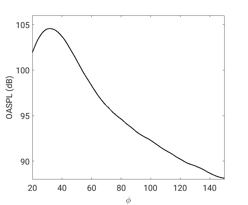
(b)

Figure 18: (a) Far-field pressure spectra for observers located $50D$ away from the nozzle exit, and (b) overall sound pressure levels as a function of polar angle.

At $100D$, the peak jet noise direction is $30^{\circ}$ to the downstream jet axis, in good agreement with experimental observations. By taking a Fourier transform of the acoustic sources in the azimuthal direction, we find that axisymmetric fluctuations comprise a large part of this peak jet noise, as shown in Fig. 18(a). At higher frequencies and higher wavenumbers, however, the contribution from axisymmetric sources diminishes in comparison to contributions from higher azimuthal wavenumbers.

IV.2 I/O analysis of LES data

In addition to sampling the LES on the FWH surface, we record data on an entire regular cylindrical mesh extending over $0<x/D<30$ and $0<r/D<9.13$. The positions of the grid points correspond exactly to the grid points used for the RANS calculations, and are uniformly spaced in the axial direction, but cluster around $r/D=0.5$ in the radial direction. We resolve this cylindrical domain by $481x180x64$ points in the axial, radial and azimuthal directions, respectively. This gives 5.5 million grid points in total, which is much smaller than the total number of cells used in the LES. We interpolate from the unstructured LES mesh to the cylindrical mesh using inverse distance weighting. Multiplying by 40 bytes (5 double precision numbers) per grid point, and 8280 time samples, the total size of the database is approximately 2 Tb.

From this database, we directly compute the Lighthill source terms lighthill1952 which are the nonlinear forcing terms driving the velocity equations (2b). Using the same Hann windows as in the FWH calculations, we analyze the frequency content using Spectral Proper Orthogonal Decomposition (SPOD) towne2018 ; schmidt2017 . Figure 19(a) shows the leading SPOD mode for axisymmetric fluctuations at $St=0.59$. The Lighthill sources involve spatial derivatives since they include the divergence of the fluctuating Reynolds stress tensor. Because of this, stochastic elements at high wavenumbers tend to be amplified. Still, Fig. 19(a) reveals significant order at this frequency, indicating the presence of non-compact sources. We would expect this order to be enhanced if SPOD analysis were applied to a quantity like pressure which tends to be more smooth in space. We should note that, in exactly the same way that acoustic analogies may be written in terms of different variables curle1955 ; goldstein2008 , different formulations of I/O analysis are possible. Some reformulations may yield source terms with desirable properties such as smoothness in space. A particularly interesting formulation may be the one based on the decomposition of Doak doak1972 recently adapted for jet noise unnikrishnan2018 , since it optimally separates the aerodynamic and acoustic components of pressure within the jet itself. Nevertheless, the Lighthill source corresponds exactly to the forcing in our I/O analysis so we focus upon it to evaluate our modes.

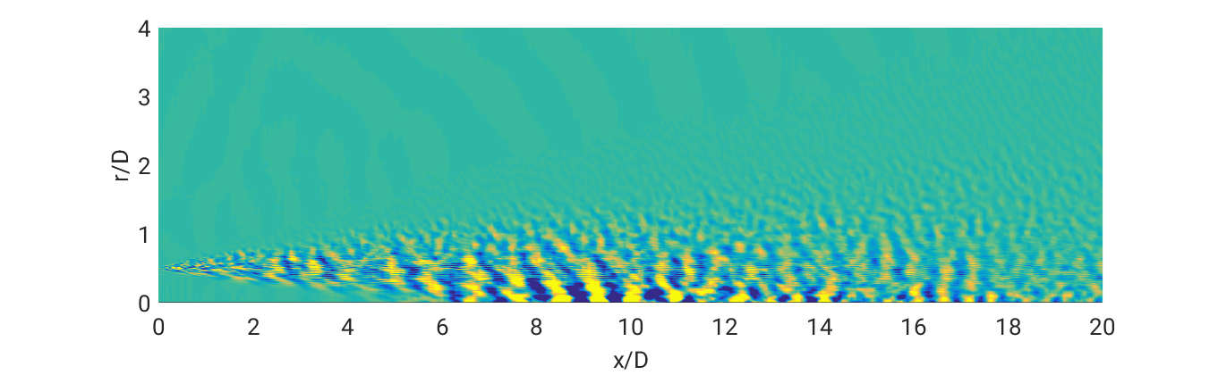
(a)

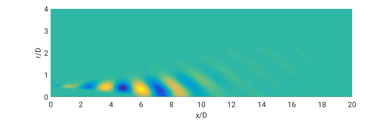
(b)

Figure 19: (a) The leading SPOD mode for axisymmetric fluctuations from the LES and (b) the optimal input forcing from I/O analysis for $m=0$ at $St=0.59$.

Figure 19(b) shows the optimal input forcing from I/O analysis at the same frequency and azimuthal wavenumber. At first glance, it seems dissimilar to the SPOD mode. To quantify this, we project the leading SPOD mode onto the orthonormal basis formed by the first 20 input modes at this frequency such that

$$\hat{q}_{LES}=\sum_{n}a_{n}\hat{q}_{in,n},$$ (21)

where $\hat{q}_{LES}$ is the Fourier transformed Lighthill source and $\hat{q}_{in,n}$ are the orthonormal input modes. The coefficients $a_{n}$ may be found simply using the following inner product with quadrature weights accounting for the non-uniform mesh.

$$a_{n}=\left<\hat{q}_{LES},\hat{q}_{in,n}\right>.$$ (22)

Figure 20(a) show the coefficients $a_{n}$ vs. mode number. Apparently, very little energy of the leading SPOD mode is captured by the input modes. This, however, is a natural consequence of the fact that very little of the aerodynamic energy contained in the turbulent fluctuations in a jet is ever radiated as sound dowling1983 . While SPOD captures the aerodynamic energy contained in the Lighthill source terms, it filters out the aeroacoustically relevant dynamics, in this case. The spatial separation of near-field inputs from far-field outputs in our I/O framework, however, means that our input modes are connected with dynamics in the jet that produce noise. If we instead first project each Fourier-transformed Hann window onto the same basis of 20 input modes, and then average the coefficients $a_{n}$, we find that they increase by three orders of magnitude (see Fig. 20(b)) compared to those obtained from projecting the SPOD mode alone. Indeed, the input modes are quite active in this jet. Moreover, the input coefficients follow a regular pattern, decreasing with input mode number, suggesting that a model for this decay may be possible. While we leave this modeling for a future study, we may interpret our input modes physically, however, as filters for the acoustically important dynamics embedded in the jet turbulence.

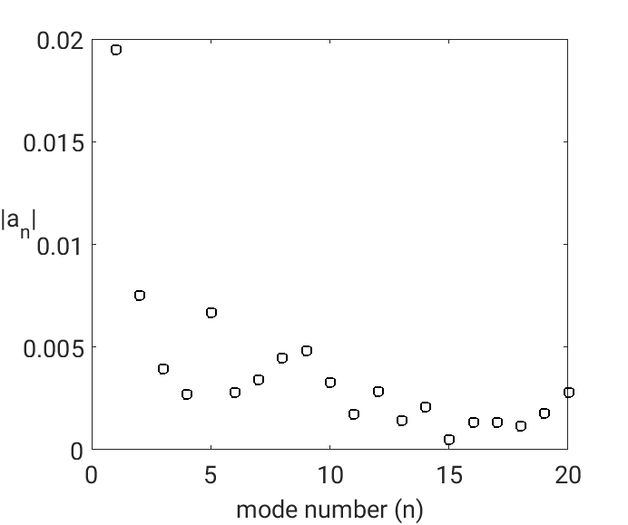
(a)

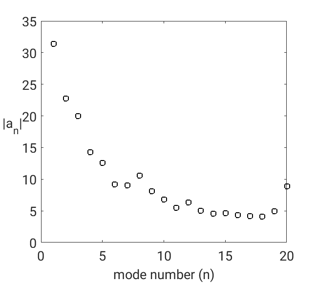
(b)

Figure 20: (The coefficients $a_{n}$ vs. mode number (a) from projecting the SPOD mode alone onto the basis of 20 input modes and (b) from projecting each Fourier-transformed Hann window and averaging the coefficients.

Using the coefficients $a_{n}$, Fig. 21 shows the reconstructed far-field sound levels obtained by superposing corresponding output modes as a function of polar angle (red curve). We compare this to the far-field sound levels from LES (blue curve). Only 20 input modes do a fairly good job at predicting both the levels and directivity of the resulting far-field sound. Evidently, the input modes do in fact capture the dynamics in the jet that produce sound.

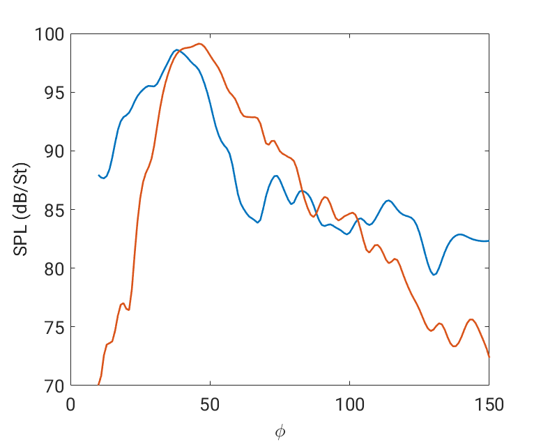
Figure 21: The reconstructed far-field sound levels by superposing corresponding output modes.

In a similar fashion, Fig. 22(a) shows the x-component of the reconstructed input forcing using the coefficients $a_{n}$. We compare this to a single Hann window of the LES data at the same frequency, shown in Fig. 22(b) (this is different from the leading SPOD mode). First, we note that the amplitude of the reconstructed input forcing is less than the amplitude of the Fourier coefficients computed from the LES data, even though the coefficients $a_{n}$ are much larger than those obtained previously. Secondly, while both the LES data and the reconstructed input show coherence, there appears to be a mismatch in the wavenumbers between the two. We quantify this difference by applying Fourier transforms in the axial direction to the two fields and average the resulting wavenumber spectra in the radial direction. Figure 23 shows the spectra obtained from both the LES data (blue line) and the reconstructed input (red line). Although the LES spectra is more broadbanded than the reconstructed input, it contains a sharp peak at $k=5.3$, from which we can estimate a convection velocity of $u_{c}=\omega/k\approx 0.7u_{j}$. The reconstructed input is focused, however, on a wavenumber that is precisely half that obtained from the LES. Its convection velocity, therefore, is $u_{c}=1.4u_{j}$, and because of this can emit acoustic radiation directly. Physically, our input modes are connected to the radiating tail of a wavepacket represented in wavenumber space freund2001 ; jordan2013 .

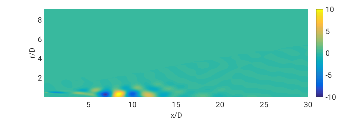
(a)

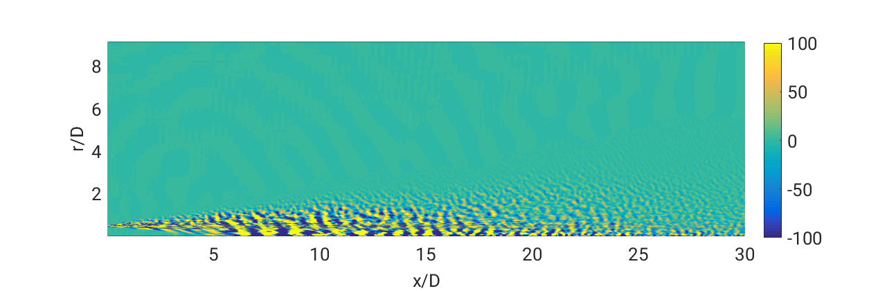
(b)

Figure 22: (a) The reconstructed input forcing for I/O analysis using the coefficients $a_{n}$; (b) The real part of the Fourier coefficients obtained at frequency $St=0.59$ for one Hann window of the LES data.

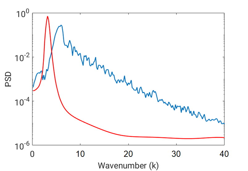
Figure 23: The spectra obtained from both the LES data (blue line) and the reconstructed input (red line).

We observe a similar spatial subharmonic relationship between LES wavepackets and the I/O modes over all frequencies. The dominant wavenumber contained in the I/O modes forcing to be precisely half that extracted from the LES data. While I/O analysis is linear, it incorporates all axial wavenumbers simultaneously as a global method, and so resolves physical waveforms that may contain subharmonic components. In the LES, these wavenumbers could couple together in time as well, through the nonlinearity of the forcing terms. Alternatively, the stochastic nature of the turbulent fluctuations in the jet could intermittently align to perturb the coherent structures contained in the jet turbulence in just the right way so that they emit sound. The optimal way to perturb wavepackets observed in the LES is given by the reconstructed input forcing shown in Fig. 22(a).

Whether or not the forcing comes from nonlinearity or stochasticity, the fact that our input modes correspond to small-amplitude, spatially subharmonic perturbations to dominant instability wavepackets suggests the physical mechanism for noise generation shown in Fig. 24. In this figure, subharmonic forcing is applied to a Gaussian wavepacket so that the peak amplitude of every other wave is slightly amplified or diminished. In terms of coherent structures in the jet, this would correspond to slight offsets in their exact positions. In other words, in subsonic jets, it is the jitter of the components of a wavepacket that is responsible for noise. This type of jitter is exactly the mechanism observed in compressible mixing by Wei and Freund, 2006 wei2006 . In their study, they applied adjoint-based optimal control to reduce the sound generated from the mixing layer by 11 dB. Remarkably, the coherent flow features (large scale vortices) of the controlled and uncontrolled simulations remained nearly identical. A slight jitter in the exact positions of the large scale flow features accounted for the only difference between the two simulations.

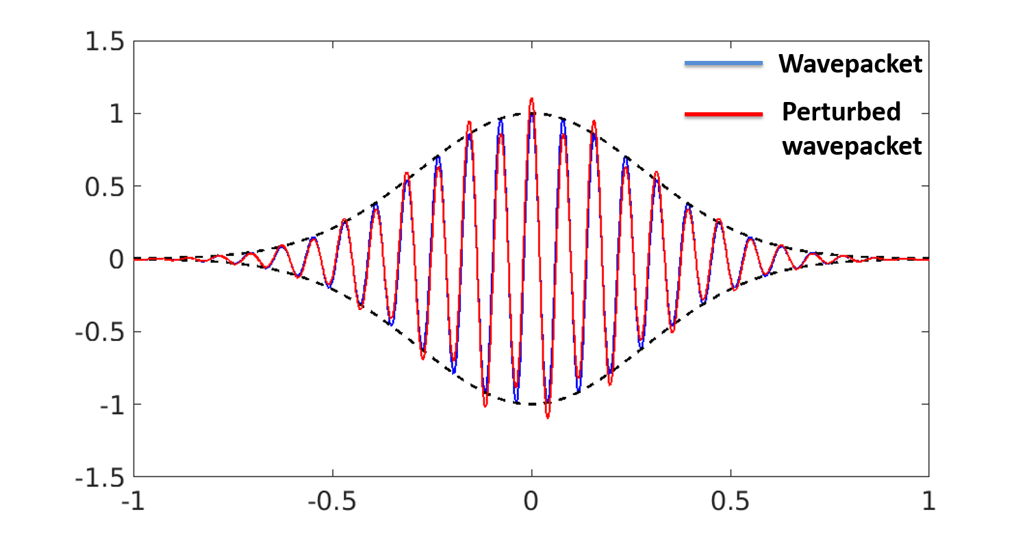
Figure 24: A Gaussian wavepacket perturbed by spatially subharmonic forcing.

To show that the subharmonic relationship between the instability wavepackets and their acoustic radiation exists in the LES data, we consider the pressure on the FWH surface used to compute far-field sound. Figure 25 shows the real part of the Fourier coefficients at a frequency of $St=0.2$ on the conical surface, which has been unwrapped in the azimuthal direction. Compared to the the Lighthill source shown in Fig. 19(a), the pressure field is much more smooth. Because the FWH surface is so close to the jet, it captures near-field pressure fluctuations created aerodynamically by an instability wavepacket. This wavepacket is evident on the upstream part of the FWH surface, close to the nozzle exit. Since they are associated with aerodynamic effects, these upstream waves do not radiate to the far-field, however, and die out exponentially in the radial direction. The downstream portion of the FWH surface captures waves with twice the wavelength. At the same frequency, these waves do radiate to the far-field and are responsible for the majority of the sound emitted by the jet at this frequency. In this particular realization, the upstream aerodynamic wavepacket upstream appears to be of helical type, whereas the noise radiated is primarily axisymmetric, further suggesting a separation between aerodynamic and aeroacoustic components of the jet dynamics.

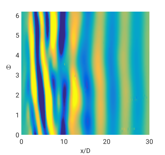
Figure 25: The real part of the Fourier coefficients at a frequency of $St=0.2$ on the conical FWH surface.

V Conclusions

In the present study we explore in detail the physics of sound generation mechanisms in a Mach 0.9 turbulent jet using coherent modes generated by I/O analysis. In the spirit of Lighthill’s acoustic analogy, a crucial aspect of our I/O formulation is the spatial separation of acoustic sources from the far-field noise they produce. Different from acoustic analogies, however, I/O analysis allows us to decompose the sources in terms of acoustically important dynamics, rather than describing them only in terms of statistical cross-correlations. Using our method, we find that the optimal sound-producing dynamics correspond to non-compact coherent sources in the form of wavepackets. In terms of their envelope, our wavepackets agree remarkably well with wavepackets measured in the near-field of turbulent jets in both laboratory experiments and simulations, and to those used in semi-empirical models. Rather than stopping at the near-field, however, I/O analysis provides a method whereby sound is traced back to its origins embedded in the jet turbulence. The wavepackets shown in this paper were obtained along the lipline of the jet.

Furthermore, we find that our wavepackets remain similar in shape over a range of frequencies. This behavior agrees well with the stochastic similarity wavepacket model papamoschou2011 , and may help explain some of its success. Rather than being inversely proportional to the frequency, however, we find that our wavepackets scale approximately as $St^{-0.5}$. Clearly, though, the optimal input modes predicted by I/O analysis are associated with self-similar instability wavepackets, and can be represented with a model of very low complexity.

For a Mach 0.9 jet, we additionally obtain a spectrum of sub-optimal modes that have nearly the same gain as the optimal mode. These sub-optimal modes follow a pattern that aligns well with modes obtained from a simple model axial decoherence of a wavepacket. Furthermore, the acoustic output of the sub-optimal involve increasingly wide angles of far-field directivity with mode number. The sub-optimal modes therefore play a key role in noise radiation at high angles to the downstream jet axis. Physically, the input modes from I/O analysis seem to correspond to decoherence modes and at the same time provide insight into the effect of decoherence on far-field noise radiation. It may be interesting to introduce a model of decoherence in place of axial uncertainty (jitter) in similarity wavepacket models of jet noise.

Projecting high-fidelity LES data onto the basis of input modes, we find that the input modes are indeed quite active. Because they are filters for aeroacoustically important dynamics, they should, however, be applied directly to the LES data before any type of averaging or decomposition is applied. When this is done, the reconstructed output acoustics match the levels and peak direction obtained from LES. This indicates that the input modes do indeed capture the acoustically relevant dynamics in the jet. Moreover, only a limited number of input modes are necessary to do this, which suggests that these noise-producing dynamics are low-dimensional in nature.

It is important to note that, relative to the energetically dominant motions in the jet, the acoustically important dynamics associated with our input modes have small energy. While the envelopes of our input modes correspond exactly to wavepacket envelopes associated with instability waves, the wavenumber of our input modes has a subharmonic relationship with the wavenumbers associated with Kelvin-Helmholtz instability. Our input modes are associated with the radiating supersonic tail of a wavepacket in wavenumber space. While this tail is created by the shape of the envelope in physical space, the fact that the wavenumber of our input modes is exactly half that of the Kelvin-Helmholtz instability educed by SPOD, suggests a physical mechanism whereby waves inside the packet are perturbed in an alternating pattern. This also explains why we recover the same envelope as instability wavepackets such as those computed by PSE: our input modes correspond to small, spatially subharmonic perturbations to instability waves. This type of noise-producing pattern has been observed previously in low Reynolds number simulations of compressible mixing layers wei2006 .

Appendix A Verification of the linearized FWH solver

We start from the permeable surface FWH equation for a stationary source in a quiescent medium lockard2000 ; lockard2005 ; bres2012 , which is given by:

$$\left(\frac{\partial^{2}}{\partial t^{2}}-c_{\infty}^{2}\frac{\partial^{2}}{\partial x_{i}\partial x_{j}}\right)\left[\left(\rho-\rho_{\infty}\right)H\left(S\right)\right]=\frac{\partial}{\partial t}\left[Q_{n}\delta\left(S\right)\right]-\frac{\partial}{\partial x_{i}}\left[F_{i}\delta\left(S\right)\right]-\frac{\partial^{2}}{\partial x_{i}\partial x_{j}}\left[T_{ij}H\left(S\right)\right],$$ (23)

where the monopole source terms $Q_{n}$, dipole source terms $F_{i}$, and the Lighthill stress tensor $T_{ij}$ are respectively defined as:

$$Q_{n} = \rho u_{i}\hat{n}_{i},$$ (24a)

$$F_{i} = \left(P_{ij}+\rho u_{i}u_{j}\right)\hat{n}_{j},$$ (24b)

$$T_{ij} = \rho u_{i}u_{j}+P_{ij}-c_{\infty}^{2}\left(\rho-\rho_{\infty}\right)\delta_{ij}.$$ (24c)

In the above equations the function $S$ defines the surface so that the solution to Eq. (23) is sought outside of the surface $S=0$, and in this regard the Heaviside function $H$ becomes unity for $S>0$ and zero for $S<0$. Furthermore, $\hat{n}_{i}$ represents a unit outward normal vector to the surface $S=0$, and $u_{i}$ is the local fluid velocities on the surface $S=0$. The total density is given by $\rho$ while the ambient properties are denoted by the subscript $\infty$. Then, perturbation properties may be distinguished by the superscript ^′ such as the density perturbation is written as $\rho^{\prime}=\rho-\rho_{\infty}$. Note in the Lighthill stress tensor the compressive stress tensor $P_{ij}$ is defined as $P_{ij}=\left(p-p_{\infty}\right)\delta_{ij}$ after neglecting the viscous term.

To perform the Fourier analysis, Eq. (23) may be re-written in more convenient form as:

$$\left(\frac{\partial^{2}}{\partial x_{j}\partial x_{j}}+k^{2}\right)\left[\left(c_{\infty}^{2}\tilde{\rho}^{\prime}\right)H\left(S\right)\right]=-\mathrm{i}\omega\tilde{Q}_{n}\delta\left(S\right)+\frac{\partial}{\partial x_{i}}\left[\tilde{F}_{i}\delta\left(S\right)\right]-\frac{\partial^{2}}{\partial x_{i}\partial x_{j}}\left[\tilde{T}_{ij}H\left(S\right)\right],\\$$ (25)

where $k$ is the wavenumber given by $k=\omega/c_{\infty}$. In fact, we may replace the term $c_{\infty}^{2}\tilde{\rho}^{\prime}$ by the pressure perturbation $p^{\prime}$ and rewrite Eq. (25) in a pressure-based form since the density perturbations are small outside of the source region spalart2009 . The integral solution is then given by:

$$\tilde{p}^{\prime}\left(\bm{x},\omega\right)=-\int_{S}\tilde{F}_{i}\left(\bm{y},\omega\right)\frac{\partial G\left(\bm{x},\bm{y}\right)}{\partial y_{i}}dS-\int_{S}\mathrm{i}\omega\tilde{Q}_{n}\left(\bm{y},\omega\right)G\left(\bm{x},\bm{y}\right)dS,$$ (26)

assuming that the volume-distributed source terms are negligibly small. Here, the three-dimensional free-space Green’s function $G$ is given by:

$$G\left(\bm{x},\bm{y}\right)=\frac{-e^{-\mathrm{i}kr}}{4\pi r}$$ (27)

where $r$ represents the distance between the source $\bm{y}$ and the observer $\bm{x}$ such that $r=|\bm{x}-\bm{y}|$. Using the chain rule, the derivative of the Green’s function with respect to the source $\bm{y}$ may be then evaluated as

$$\frac{\partial G}{\partial y_{i}}=\frac{\partial G}{\partial r}\frac{\partial r}{\partial y_{i}},$$ (28)

and in cylindrical coordinates we use here, $\frac{\partial r}{\partial y_{i}}$ is simply:

$$\frac{\partial r}{\partial y_{i}}=-\hat{r}_{i}=\frac{x_{i}-y_{i}}{|x_{i}-y_{i}|}.$$ (29)

Now we linearize the integral solution in Eq. (26) to implement a FWH solver within I/O analysis framework. Since outside of the hydrodynamic region $r/D>3$, local properties are mostly perturbation properties, we may neglect the second-order terms in the dipole source term $F_{i}$ and rewrite it as:

$$F_{i}=P_{ij}\hat{n}_{j}.$$ (30)

The linear monopole source term $Q_{n}$ remains unchanged as it is in Eq. (24).

For a FWH projection surface, we select a straight cylinder with radius $r/D=6$ whose axis lies along the jet centerline. The projection surface is thus located much closer to the jet than the Kirchhoff surface in earlier study jeun2016 was, and yet it is far enough to enclose all noise sources. The cylindrical projection surface extends from $x/D=-5$ to $x/D=35$ axially, and an outflow disk is neither closed nor equipped with end-caps. We still expect that spurious modes will not contaminate the acoustic response since the projection surface is sufficiently long and lean, and this assumption is tested for the following two cases.

A.1 Case 1: Monopole

In this appendix we validate the FWH formulation that are directly implemented within I/O analysis framework as a linear operator inside the matrix $C$, by testing a simple case for which an analytic solution exists. We consider a point monopole source located at the origin. The far-field pressure at $r$ radiated from the source is exactly written as:

$$\frac{p_{exact}(r,\omega)}{p_{ref}}=\frac{e^{-\mathrm{i}kr}}{4\pi r},$$ (31)

using the free-space Green’s function given in Eq. (27). Being consistent with notations used in the main sections, the distance between the source $\bm{y}$ and the observer $\bm{x}$ is given by $r=\left|\bm{x}-\bm{y}\right|$. The reference pressure is set to be $p_{ref}=10^{-6}$. Furthermore, $\omega$ represents the frequency and $k$ denotes the wavenumber such that $k=2\pi/\lambda$. The wavelength $\lambda$ is given as $1D$ and the speed of sound $c=1/1.5=0.6667$. Note that sound radiated from a monopole is omnidirectional so the exact solution above is independent of an azimuthal angle $\theta$. The velocity field of a monopole source is obtained by substituting this into the conservation of momentum, and then used in the linearized FWH formulation given in Eq. (26).

We place a straight cylindrical FWH projection surface so that its axis lies along the $x$-axis as shown in Fig. 26. We choose the projection surface with radius $R_{s}=3D$, which extends from $x=-15D$ to $15D$ so that its length $L_{s}=30D$. The number of grid points in the axial, radial, and azimuthal directions are given by $N_{x}=481$, $N_{r}=125$, and $N_{\theta}=64$, respectively. The grid are uniform in the streamwise and azimuthal directions but stretched in the radial direction. Meanwhile, to assess the effects of open outflow disk, we test FWH surfaces equipped with and without end-caps shur2005 , when computing the far-field pressure fields. The results are summarized in Fig. 27.

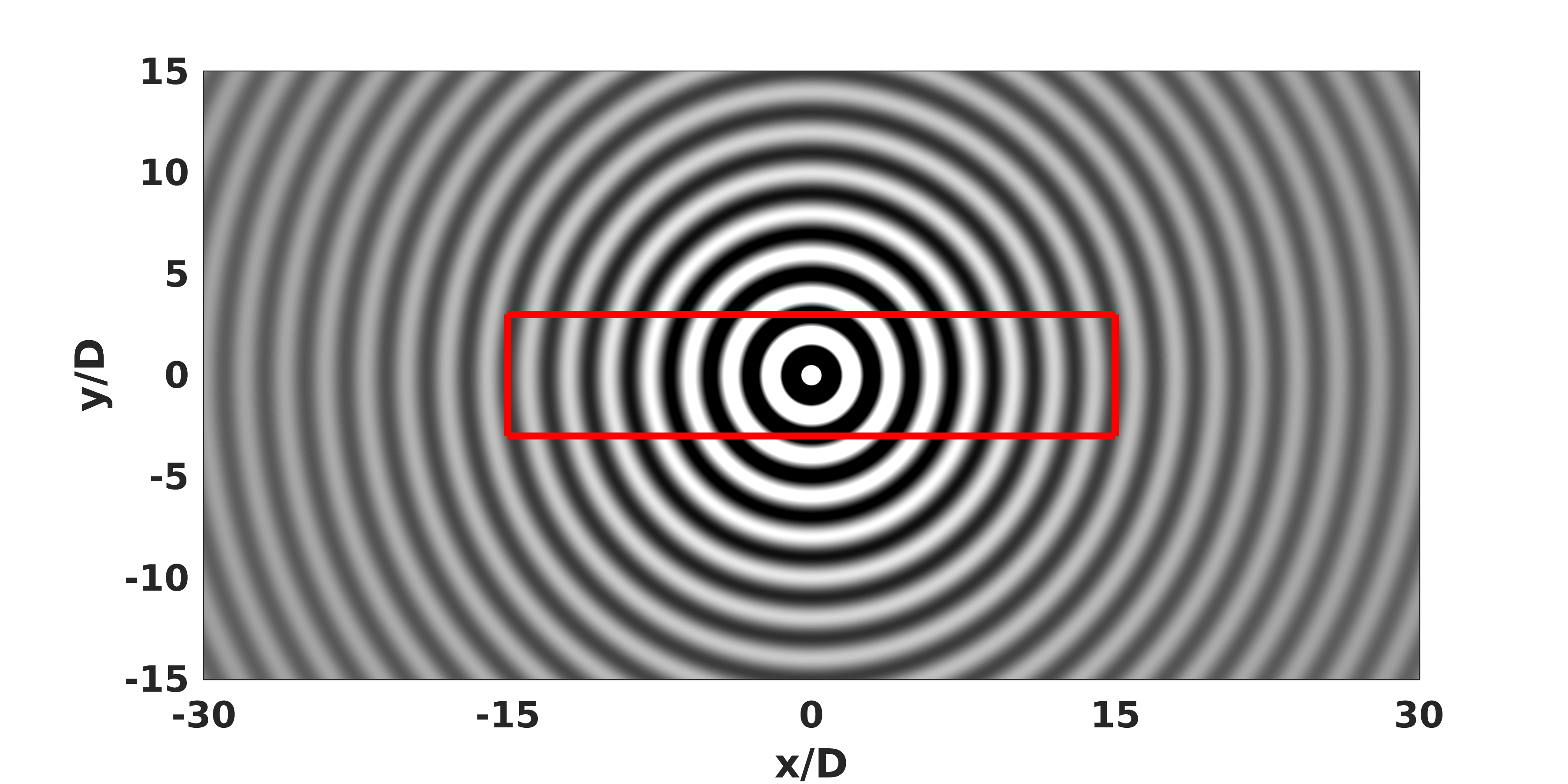
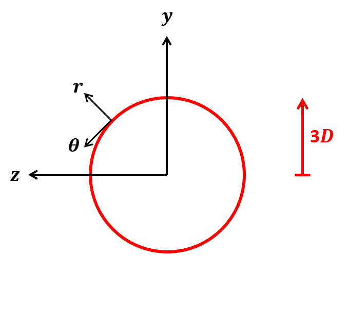
(a)	(b)

Figure 26: (a) A straight cylindrical FWH surface (a red-outlined rectangle) placed in a monopole field on $xy$-plane cross-section at $z=0$. The length of the projection surface is $30D$, and the diameter of its cross-section is $3D$. (b) A cross-sectional view of the projection surface on $yz$-plane is zoomed-in. The azimuthal angle $\theta$ is measured in a counter-clockwise direction.

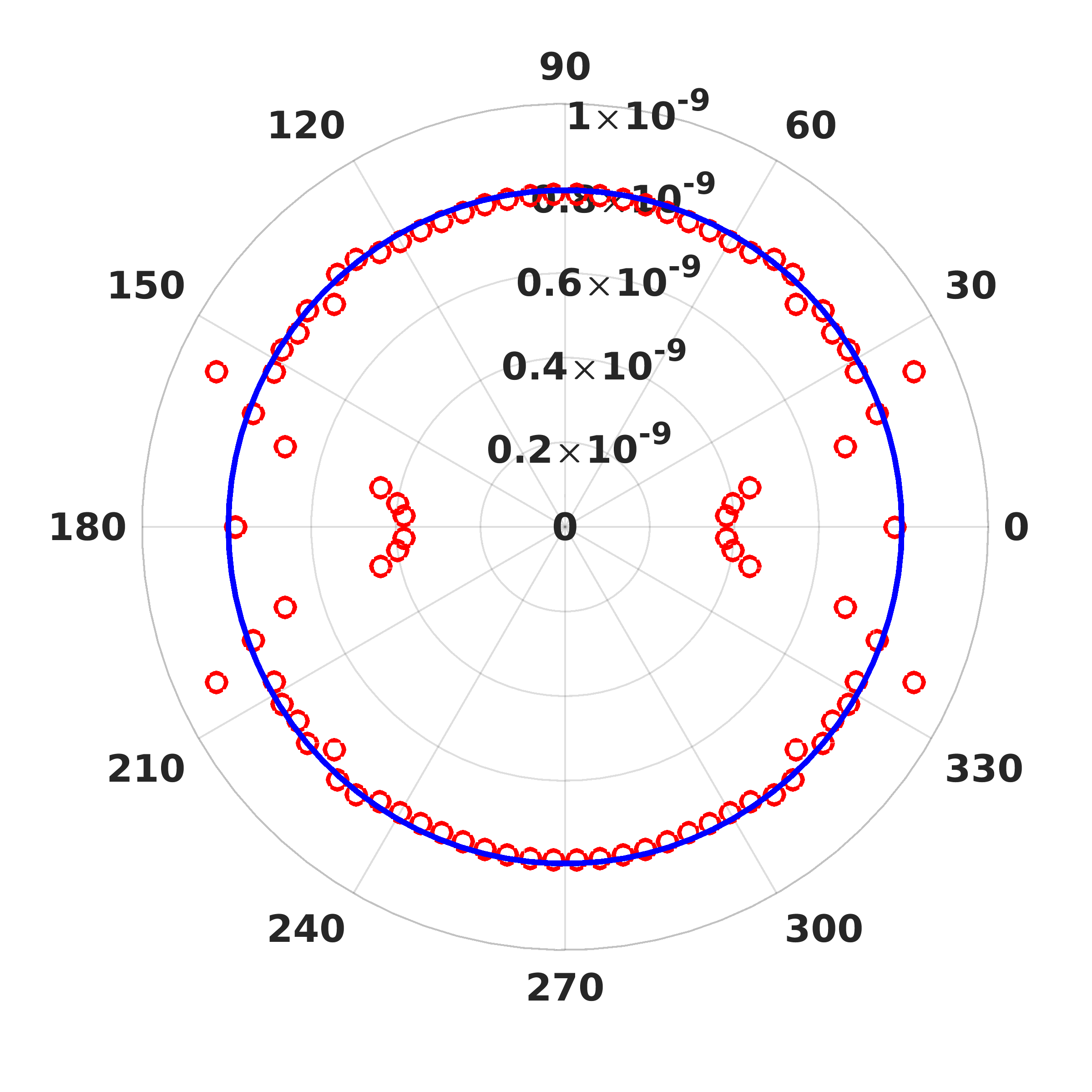
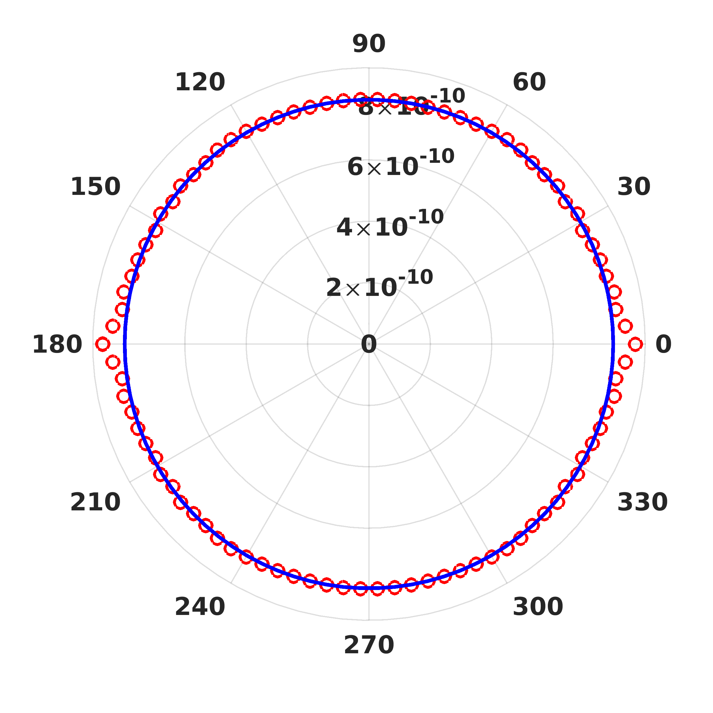
(a) Open outflow disks	(b) Closed outflow disks

Figure 27: Acoustic far-field measured at 100 diameters away from a monopole centered at the origin using the projection surfaces whose outflow disks are (a) left open and (b) closed with end-caps, respectively. In each figure blue solid line represents the exact solution, and red markers are computed using a FWH formulation implemented inside I/O analysis framework.

In Fig. 27 the blue solid lines correspond to the exact far-field sound pressure, whereas red symbols represent solutions computed using the FWH solver implemented as a linear operator. If they are left open, the numerical solutions at small radiation angles ($-20^{\circ}<\phi<20^{\circ}$ and $160^{\circ}<\phi<220^{\circ}$) deviate from the exact solution but agree fairly well elsewhere as shown in Fig. 27(a). In contrast, by closing the outflow disks the projection surface, Fig. 27(b) reproduces the exact solution at almost all observer angles.

Now, a monopole source is still placed at the origin, but the FWH projection is centered at $x/D=10D$ to mimic the flow configuration of turbulent jets we consider in this dissertation. Considering that in I/O analysis while turbulent jets enter to a quiescent fluid at $x/D=0$, the numerical domain extends from $x/D=-10$ to 40, new projection surface is not symmetric any longer about an acoustic source in streamwise direction. The schematic view of a point monopole source located at the origin and an asymmetric projection surface is given in Fig. 28. Under this condition, the linearized FWH solver recovers the far-field pressure very closely to the analytic solution at radiation angles of our interests as shown in Fig. 29 regardless of the types of outflow disks. We lose the symmetry of the pressure field and compromise some accuracy at small observer angles, but the results are still within acceptable accuracy.

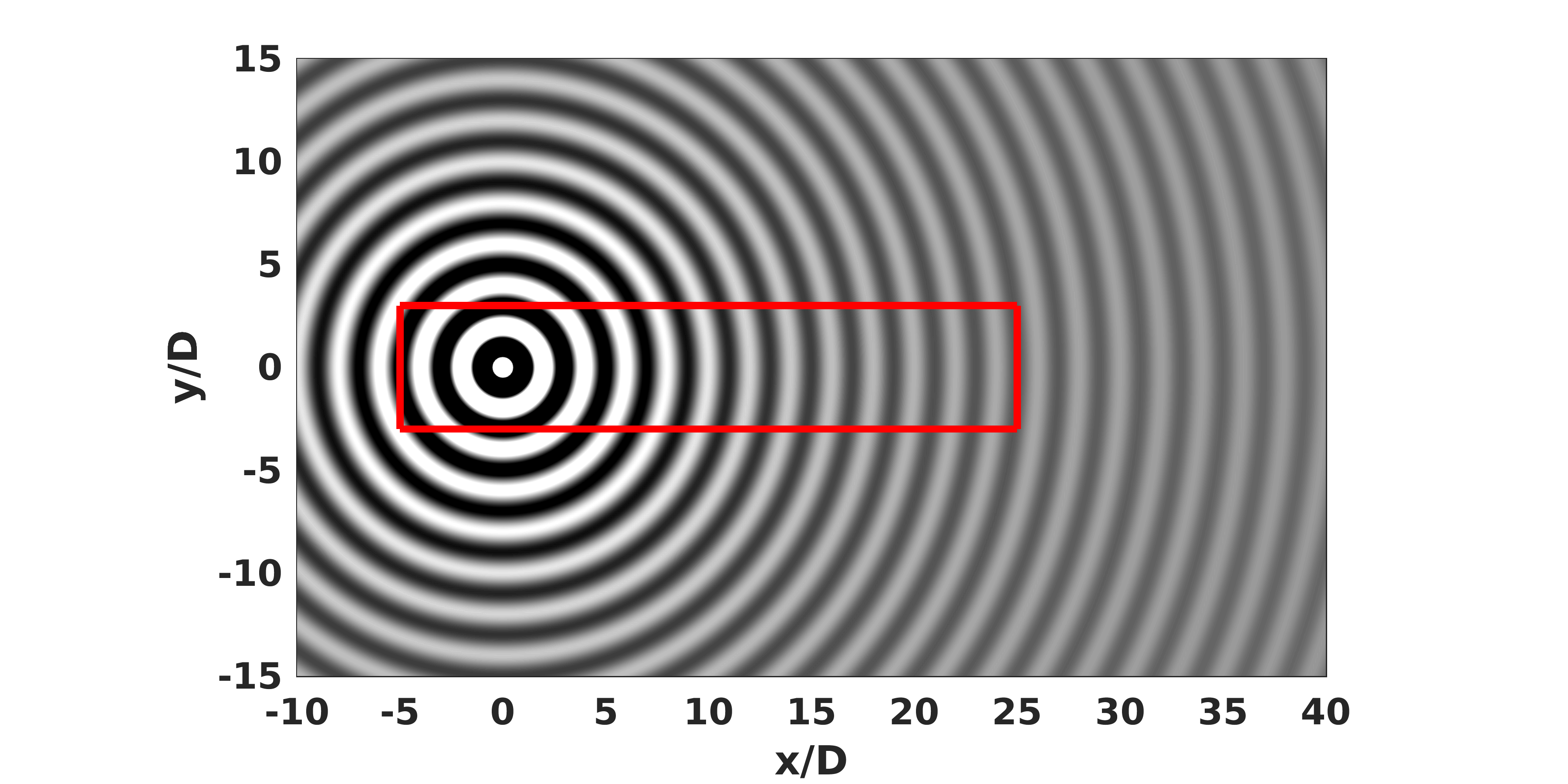
Figure 28: A straight cylindrical FWH surface (a red-outlined rectangle) is now asymmetric about a point monopole centered at the origin. The length and diameter of the projection surface remain unchanged as in the previous case.

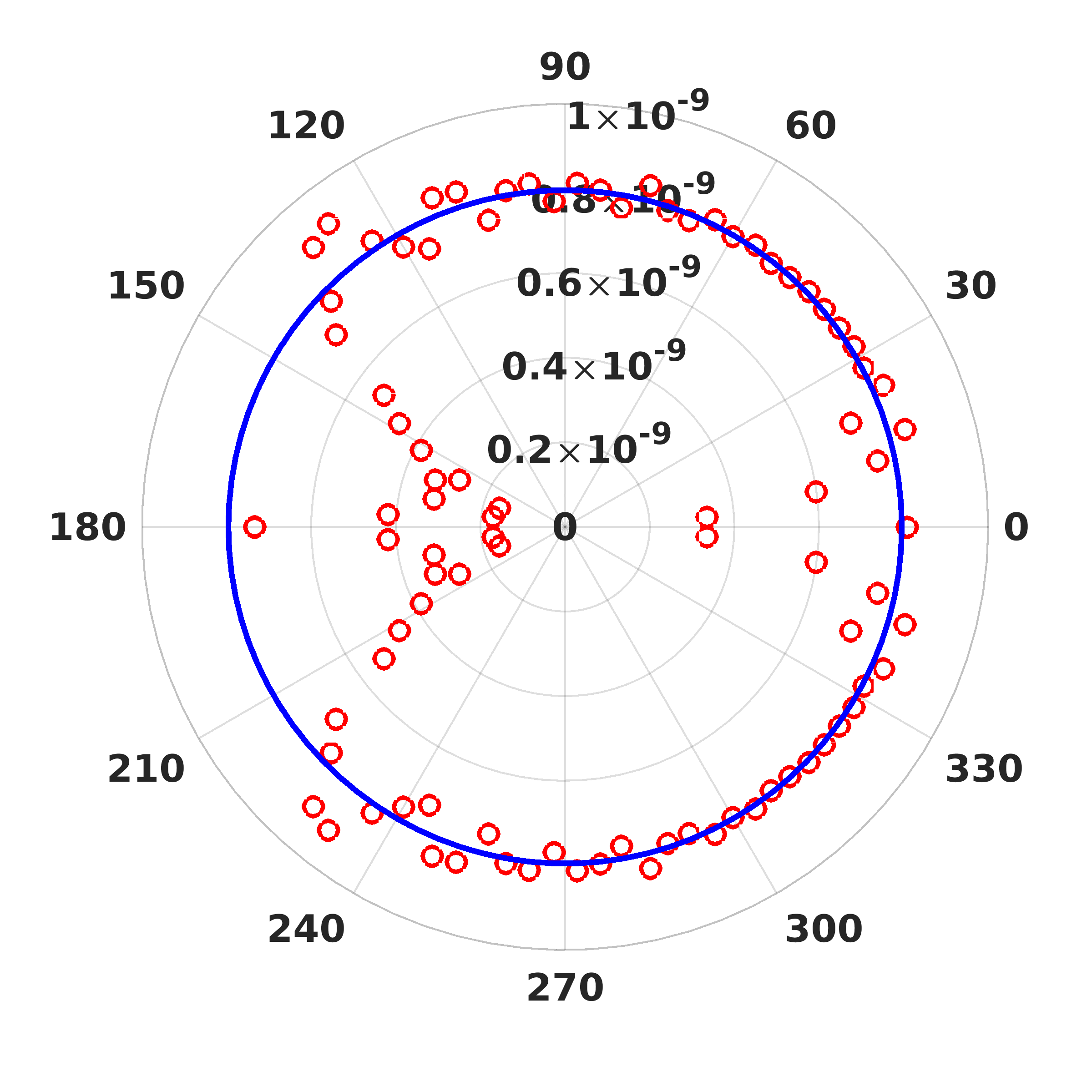
(a) Open outflow disks	(b) Closed outflow disks

Figure 29: Acoustic far-field measured at 100 diameters away from a monopole placed at 5 diameters away from the left-end of the FWH projection surface. Pressures (red markers) are predicted using (a) open and (b) closed outflow disks, respectively, and compared to the analytic solution represented by blue solid lines.

A.2 Case 2: Dipole

As seen in Eq. 26, the far-field sound is represented by surface integrals of monopole and dipole sources. In this sense we also test the linearized FWH solver with sound radiation from a dipole source. We consider a dipole source located along the $y$-axis as shown in Fig. 30. The analytic solution for a pressure field is then derived by differentiating the free-space Green’s function (27) in $y$ such as:

$$\frac{p_{exact}(r,\omega)}{p_{ref}}=\frac{\partial G}{\partial y}=\frac{\partial G}{\partial r}\frac{\partial r}{\partial y}=\frac{e^{-\mathrm{i}kr}}{4\pi r}\left(-\mathrm{i}k-\frac{1}{r}\right)\frac{\partial r}{\partial y}.$$ (32)

In cylindrical coordinates we use here, $\frac{\partial r}{\partial y}$ is conveniently computed as $\frac{y}{r}$. The reference pressure remain unchanged as $p_{ref}=10^{-6}$. The wavelength $\lambda$ is still given as $1D$, but at this time we change the speed of sound to $c=1/0.9=1.111$.

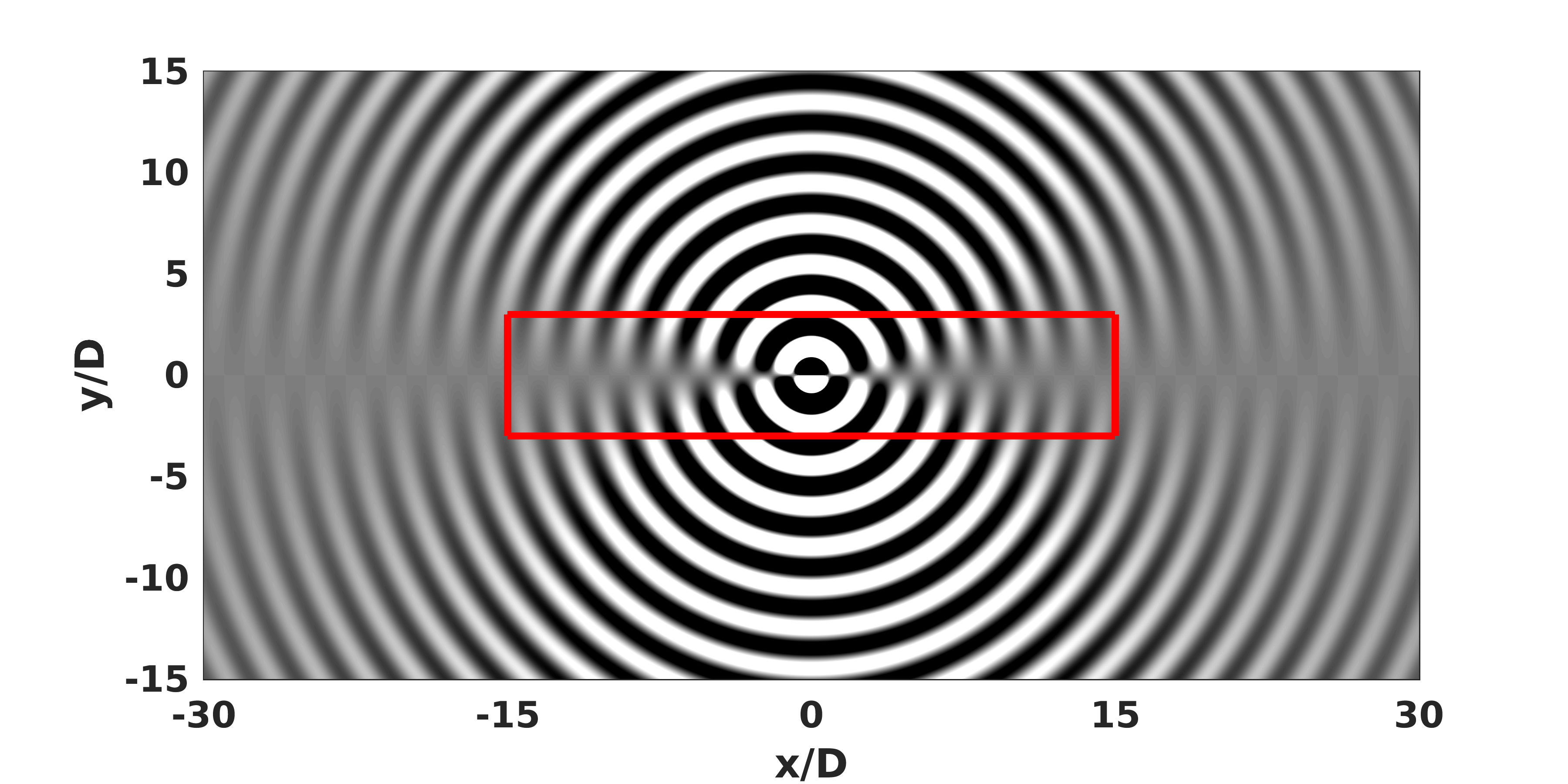
Figure 30: A straight cylindrical FWH surface for sound radiation of a dipole centered at the origin.

We use the same FWH projection surface, which was used in the previous section to test sound radiation from a monopole acoustic source. Again, a cylindrical projection surface may be either open or closed at $x/D=30$. The dipole fields obtained using different outflow disk options on the projection surfaces are compared to the exact solution (denoted by blue solid lines) in Fig. 31. The far-field acoustic predictions in both cases show reasonably good agreements with the exact solution except for the observers very close to the $x$-axis.

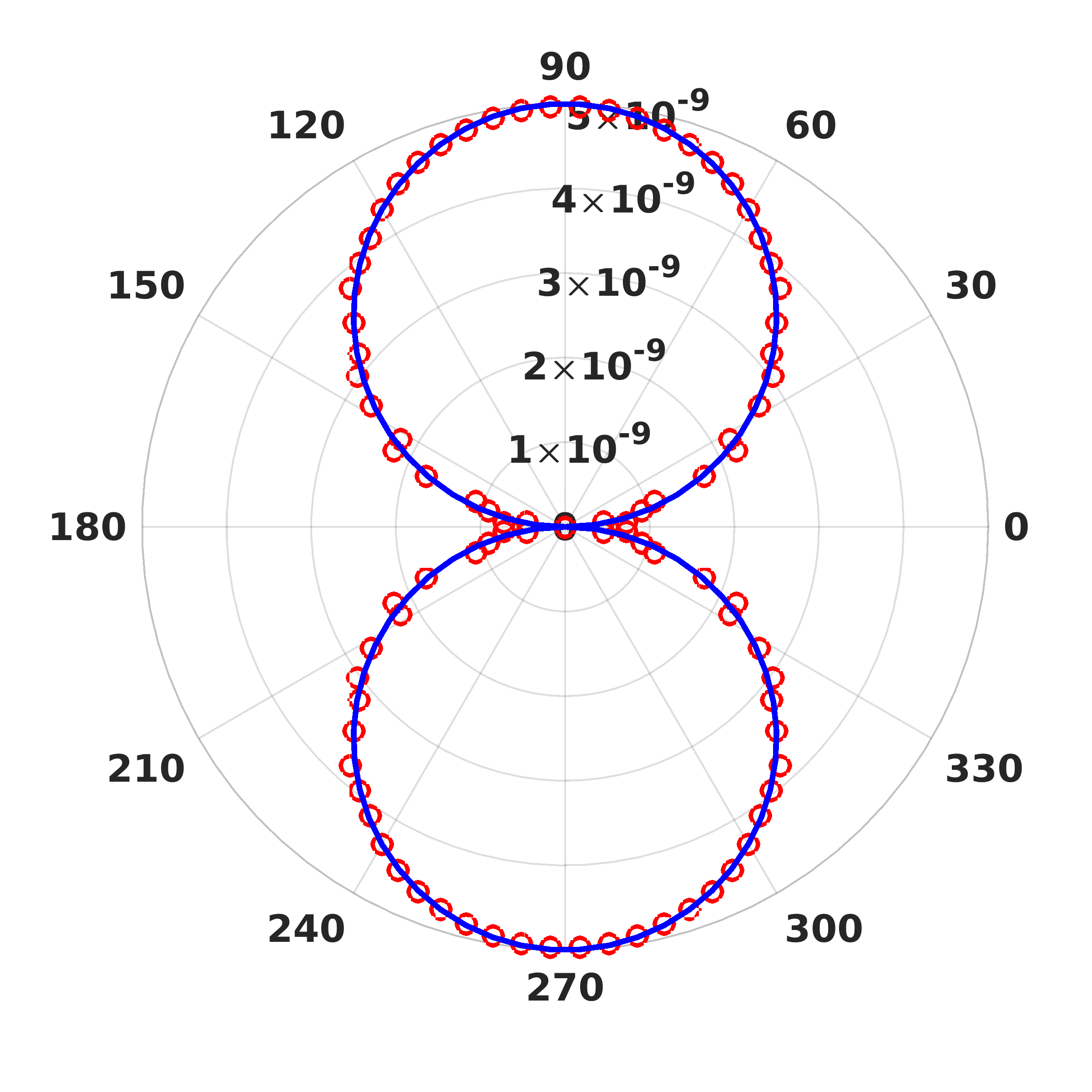
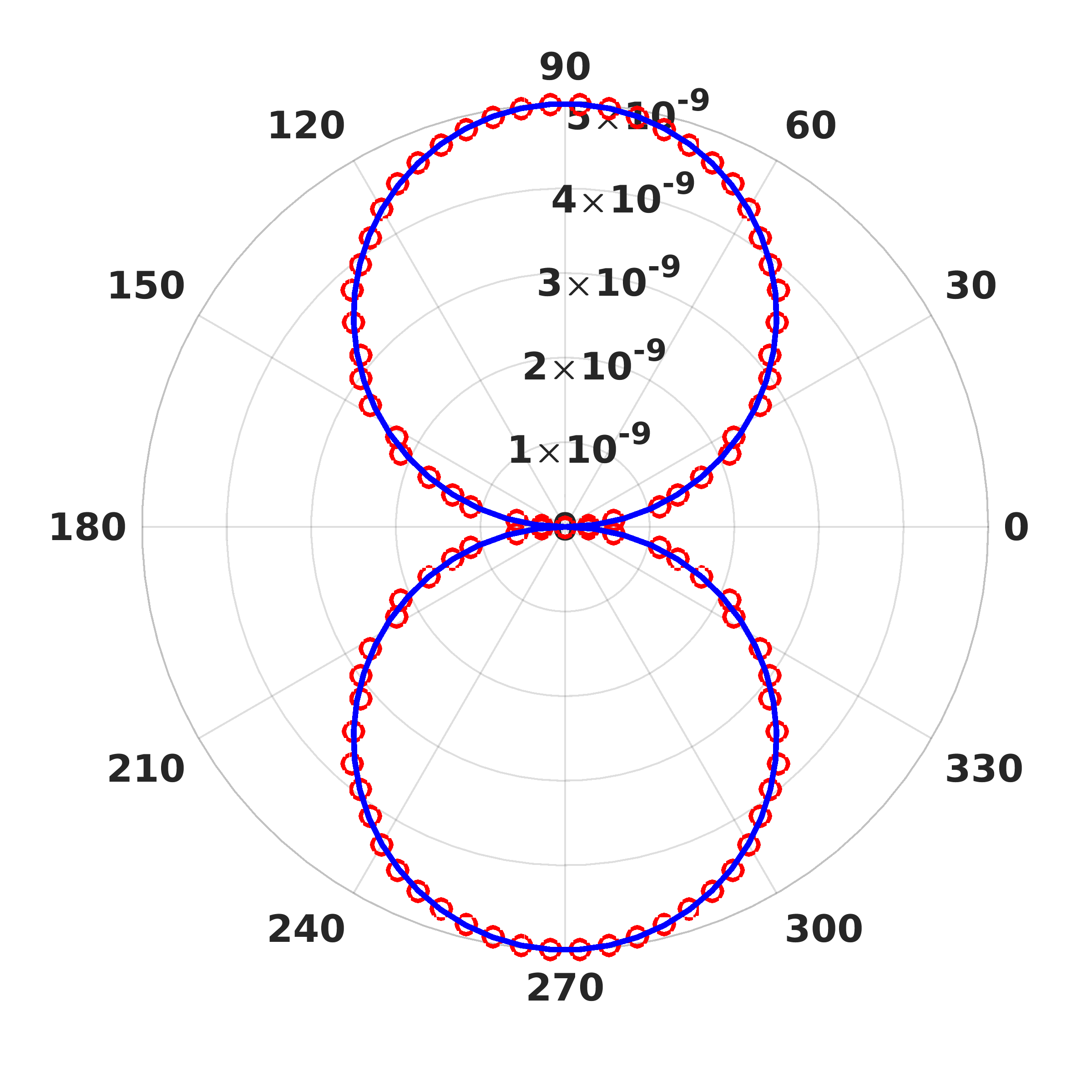
(a) Open outflow disks	(b) Closed outflow disks

Figure 31: Dipole field is measured in terms of pressure at 100 diameters away from the origin. The outflow disks of the projection surfaces are (a) left open and (b) closed with an end-cap. In each figure blue solid line represents the exact solution, and red markers are computed using a FWH formulation implemented inside I/O analysis framework.

Similarly in the case of a point monopole, we investigate the effect of asymmetric projection surface about a point dipole centered at the origin. In Fig. 32, the predictions by the linearized FWH solver are in good agreement with the analytic solution. Errors at small angles are decreased significantly with end-caps at $x/D=-5$ and $x/D=25$ even with the asymmetric projection surface.

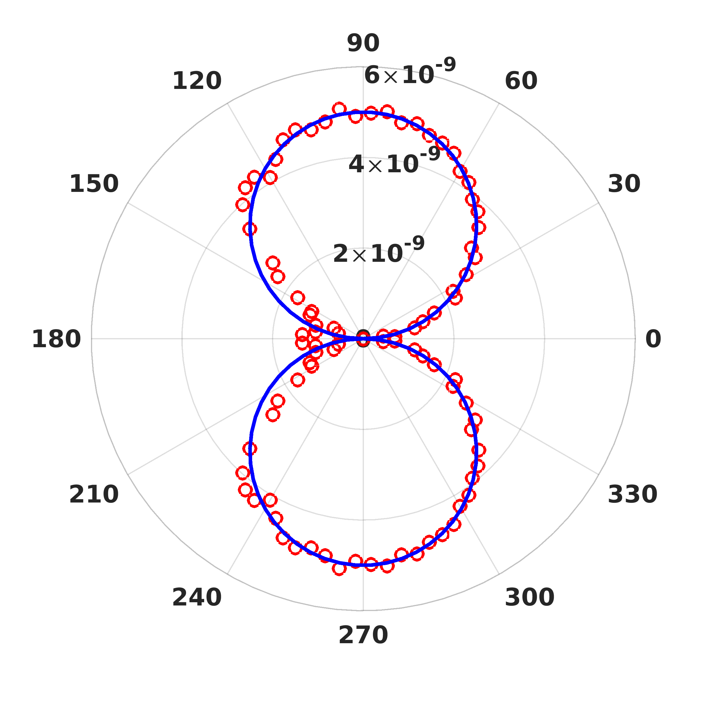
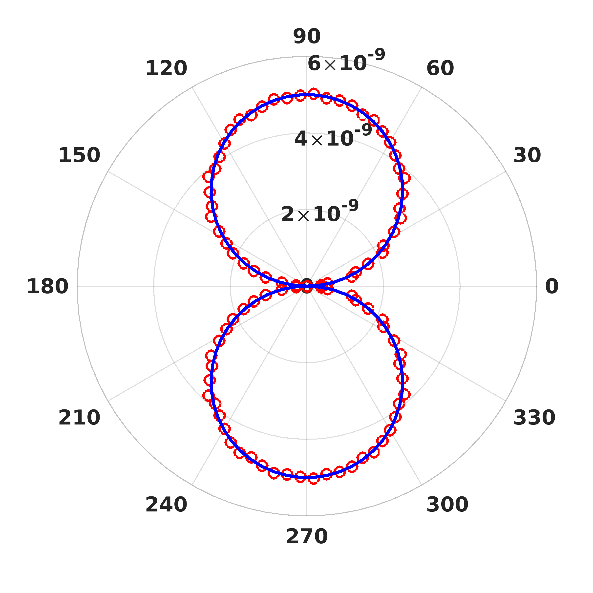
(a) Open outflow disks	(b) Closed outflow disks

Figure 32: Acoustic far-field measured at 100 diameters away from a dipole placed at 5 diameters away from the left-end of the FWH projection surface along $y$-axis. Pressures (red markers) are predicted using (a) open and (b) closed outflow disks, respectively, and compared to the analytic solution represented by blue solid lines. Equipped with end-caps at both ends of the projection surface, the predictions are significantly enhanced.

In sum, for turbulent jets, regions of low radiation angles correspond to regions that are close to the jet centerline, and we do not expect much output sound there. Based on the tests given in the previous and the present sections, we thus conclude that for a long and lean enough cylindrical projection surface, the FWH formulation implemented inside the input matrix $C$ would work even without end-cap treatments. From this, a linearized FWH solver employs an open FWH projection surface, for convenience.

References

- (1) M. J. Lighthill, “On sound generated aerodynamically. I. general theory,” Proc. Royal Soc. Lond. A 211, 564 (1952).
- (2) N. Curle, “The influence of solid boundaries upon aerodynamic sound,” Proc. Royal Soc. Lond. A 231, 505 (1955).
- (3) O. M. Phillips, “On the generation of sound by supersonic turbulent shear layers,” J. Fluid Mech. 9, 1 (1960).
- (4) J. E. Ffowcs Williams, “The noise from turbulence convected at high speed,” Proc. Royal Soc. Lond. A 255, 469 (1963).
- (5) G. M. Lilley, On the noise from jets, AGARD-CP-131 (Advisory Group for Aeronautical Research and Development, 1974).
- (6) M. E. Goldstein, “A generalized acoustic analogy,” J. Fluid Mech. 488, 315 (2003).
- (7) E. Mollo-Christensen, Measurements of near field pressure of subsonic jets, Tech. Rep. (Advisory Group for Aeronautical Research and Development, 1963).
- (8) E. Mollo-Christensen, “Jet noise and shear flow instability seen from an experimenter′s viewpoint,” J. Applied Mech. 34, 1 (1967).
- (9) S. C. Crow and F. H. Champagne, “Orderly structure in jet turbulence,” J. Fluid Mech. 48, 547 (1971).
- (10) A. Michalke, A wave model for sound generation in circular jets, (Deutsche Luft- und Raumfahrt, 1970).
- (11) A. Michalke, “An expansion scheme for the noise from circular jets,” Z. Flugwiss. 20, 229 (1972).
- (12) G. E. Mattingly and C. C. Chang, “Unstable waves on an axisymmetric jet column,” J. Fluid Mech. 65, 541 (1974).
- (13) D. G. Crighton and M. Gaster, “Stability of slowly diverging jet flow,” J. Fluid Mech. 77, 397 (1976).
- (14) A. Michalke, “Survey on jet instability theory,” Prog. Aerosp. Sci. 21, 159 (1984).
- (15) C. K. W. Tam and D. E. Burton, “Sound generated by instability waves of supersonic flows. Part 2. Axisymmetric jets,” J. Fluid Mech. 138, 273 (1984).
- (16) T. Suzuki and T. Colonius, “Instability waves in a subsonic round jet detected using a near-field phased microphone array,” J. Fluid Mech. 565, 197 (2006).
- (17) P. Jordan and T. Colonius, “Wave packets and turbulent jet noise,” Annu. Rev. Fluid Mech. 45, 173 (2013).
- (18) H. V. Fuchs, “Measurement of pressure fluctuations within subsonic turbulent jets,” J. Sound Vib. 22, 361 (1972).
- (19) H. V. Fuchs, “Space correlations of the fluctuating pressure in subsonic turbulent jets,” J. Sound Vib. 23, 77 (1972).
- (20) J. Seiner and G. Reethof, “On the distribution of source coherency in subsonic jets,” AIAA Paper 74-4 (1974).
- (21) R. R. Armstrong, A. Michalke, and H. V. Fuchs, “Coherent structures in jet turbulence and noise,” AIAA J. 15, 1011 (1977).
- (22) C. J. Moore, “The role of shear-layer instability waves in jet exhaust noise,” J. Fluid Mech. 80, 321 (1977).
- (23) R. Reba, S. Narayanan, and T. Colonius, “Wave-packet models for large-scale mixing noise,” Int. J. Aeroacoust. 9, 533 (2010).
- (24) A. V. G. Cavalieri, P. Jordan, T. Colonius, and Y. Gervais, “Axisymmetric superdirectivity in subsonic jets,” J. Fluid Mech. 704, 388 (2012).
- (25) J. B. Freund, “Noise sources in a low-Reynolds-number turbulent jet at Mach 0.9,” J. Fluid Mech. 438, 277 (2001).
- (26) L. C. Cheung, D. J. Bodony, and S. K. Lele, “Noise radiation predictions from jet instability waves using a hybrid nonlinear PSE-acoustic analogy approach,” AIAA Paper 2007-3638 (2007).
- (27) K. Gudmundsson and T. Colonius, “Instability wave models for the near-field fluctuations of turbulent jets,” J. Fluid Mech. 689, 97 (2011).
- (28) D. Rodríguez, A. Sinha, G. A. Brès, and T. Colonius, “Inlet conditions for wave packet models in turbulent jets based on eigenmode decomposition of large eddy simulation data,” Phys. Fluids 25, 105107 (2013).
- (29) A. Sinha, D. Rodríguez, G. A. Brès, and T. Colonius, “Wavepacket models for supersonic jet noise,” J. Fluid Mech. 742, 71 (2014).
- (30) J. W. Nichols and S. K, “Global modes and transient response of a cold supersonic jet,” J. Fluid Mech. 669, 225 (2011).
- (31) P. J. Schmid and D. S. Henningson, Stability and Transition in Shear Flows (Springer, New York, 2001).
- (32) X. Garnaud, L. Lesshafft, P. J. Schmid, and P. Huerre, “The preferred mode of incompressible jets: linear frequency response analysis,” J. Fluid Mech. 716, 189 (2013).
- (33) J. W. Nichols and M. R. Jovanović, “Input-output analysis of high-speed jet noise,” in Proceedings of the Summer Program (Center for Turbulence Research, Stanford University) pp. 251–260.
- (34) J. Jeun, J. W. Nichols, and M. R. Jovanović, “Input-output analysis of high-speed axisymmetric isothermal jet noise,” Phys. Fluids 28, 047101 (2016).
- (35) A. Michalke, “On the effect of spatial source coherence on the radiation of jet noise,” J. Sound Vib. 55, 377 (1977).
- (36) D. G. Crighton and P. Huerre, “Shear-layer pressure fluctuations and superdirective acoustic sources,” J. Fluid Mech. 220, 355 (1990).
- (37) Y. B. Baqui, A. Agarwal, A. V. G. Cavalieri, and S. Sinayoko, “A coherence-matched linear source mechanism for subsonic jet noise,” J. Fluid Mech. 776, 235 (2015).
- (38) R. Serré, J.-C. Robinet, and F. Margnat, “The influence of a pressure wavepacket′s characteristics on its acoustic radiation,” J. Acoust. Soc. Am. 137, 3178 (2015).
- (39) C. K. W. Tam, M. Golebiowski, and J. M. Seiner, “On the two components of turbulent mixing noise from supersonic jets,” AIAA Paper 96-1716 (1996).
- (40) S. A. Karabasov, “Understanding jet noise,” Proc. Royal Soc. Lond. A 368, 3593 (2010).
- (41) D. Papamoschou, “Wavepacket modeling of the jet noise source,” AIAA Paper 2011-2835 (2011).
- (42) A. P. Dowling and J. E. Ffowcs Williams, Sound and sources of sound (Horwood, 1983).
- (43) M. L. Shur, P. R. Spalart, and M. Kh. Strelets, “Noise prediction for increasingly complex jets. Part I: Methods and tests,” Int. J. Aeroacoust. 4, 213 (2005).
- (44) A. V. G. Cavalieri, P. Jordan, A. Agarwal, and Y. Gervais, “Jittering wave-packet models for subsonic jet noise,” J. Sound Vib. 330, 4474 (2011).
- (45) A. V. G. Cavalieri, G. Daviller, P. Comte, P. Jordan, G. Tadmor, and Y. Gervais, “Using large eddy simulation to explore sound-source mechanisms in jets,” J. Sound Vib. 330, 4098 (2011).
- (46) G. A. Brès, V. Jaunet, M. Le Rallic, P. Jordan, T. Colonius, and S. K. Lele, “Large eddy simulation for jet noise: the importance of getting the boundary layer right,” AIAA Paper 2015-2535 (2015).
- (47) P. Jordan, T. Colonius, G. A. Brès, M. Zhang, A. Towne, and S. K. Lele, “Modeling intermittent wavepackets and their radiated sound in a turbulent jet,” in Proceedings of the Summer Program (Center for Turbulence Research, Stanford University, 2014) pp. 241–249.
- (48) C. K. W. Tam, “Supersonic jet noise,” Annu. Rev. Fluid Mech. 27, 17 (1995).
- (49) A. T. Thies and C. K. W. Tam, “Computation of turbulent axisymmetric and nonaxisymmetric jet flows using the k- model,” AIAA J. 34, 309 (1996).
- (50) J. W. Nichols, S. K. Lele, and P. Moin, Global mode decomposition of supersonic jet noise, Annual Research Briefs (Center for Turbulence Reearch, Stanford University, 2009).
- (51) Y. Khalighi, A. Mani, F. Ham, and P. Moin, “Prediction of sound generated by complex flows at low Mach numbers,” AIAA J. 48, 306 (2010).
- (52) A. Mani, “Analysis and optimization of numerical sponge layers as a nonreflective boundary treatment,” J. Comput. Phys. 231, 704 (2012).
- (53) R. B. Lehoucq, D. C. Sorensen, and C. Yang, Users′ Guide: Solution of Large-Scale Eigenvalue Problems with Implicitly Restarted Arnoldi Methods (SIAM, 1998).
- (54) X. S. Li and J. W. Demmel, “SuperLUDIST: A scalable distributed-memory sparse direct solver for unsymmetric linear systems,” ACM Trans. Math. Softw. 29, 110 (2003).
- (55) J. Jeun and J. W. Nichols, “Non-compact sources of sound in high-speed turbulent jets using input-output analysis,” AIAA Paper 2018-#### (2018).
- (56) D. Papamoschou, “Prediction of jet noise shielding,” AIAA Paper 2010-0653 (2010).
- (57) A. V. G. Cavalieri and A. Agarwal, “Coherence decay and its impact on sound radiation by wavepackets, J. Fluid Mech. 748, 399 (2014).
- (58) K. B. M. Q. Zaman, “Effect of initial boundary-layer state on subsonic jet noise,” AIAA J. 50, 1784 (2012).
- (59) G. A. Brès, J. W. Nichols, S. K. Lele, and F. E. Ham, “Towards best practices for jet noise predictions with unstructured large eddy simulations,” AIAA Paper 2012-2965 (2012).
- (60) D. P. Lockard, “An efficient, two-dimensional implementation of the Ffowcs Williams and Hawkings equation,” J. Sound Vib. 229, 897 (2000).
- (61) D. P. Lockard and J. Casper, “Permeable surface corrections for Ffowcs Williams and Hawkings integrals,” AIAA Paper 2005-2995 (2005).
- (62) P. Welch, “The use of fast fourier transform for the estimation of power spectra: A method based on time averaging over short, modified periodograms,” IEEE Trans. Audio Electroacoust. 15, 70 (1967).
- (63) C. Bogey, S. Barré, V. Fleury, C. Bailly, and D. Juvé, “Experimental study of the spectral properties of near-field and far-field jet noise,” Int. J. Aeroacoust. 6, 73 (2007).
- (64) A. Towne, O. T. Schmidt, and T. Colonius, “Spectral proper orthogonal decomposition and its relationship to dynamic mode decomposition and resolvent analysis,” J. Fluid Mech. 847, 821 (2018).
- (65) O. T. Schmidt, A. Towne, G. Rigas, T. Colonius, and G. A. Brès, “Spectral analysis of jet turbulence,” arXiv preprint arXiv:1711.06296 (2017).
- (66) M. E. Goldstein and S. J. Leib, “The aeroacoustics of slowly diverging supersonic jets,” J. Fluid Mech. 600, 291 (2008).
- (67) P. E. Doak, “Analysis of internally generated sound in continuous materials: 2. a critical review of the conceptual adequacy and physical scope of existing theories of aerodynamic noise, with special reference to supersonic jet noise,” J. Sound Vib. 25, 263 (1972).
- (68) S. Unnikrishnan and D. V. Gaitonde, “Transfer mechanisms from stochastic turbulence to organized acoustic radiation in a supersonic jet,” European J. Mech. B/Fluids 72, 38 (2018).
- (69) M. Wei and J. B. Fruend, “A noise-controlled free shear flow,” J. Fluid Mech. 546, 123 (2006).
- (70) P. R. Spalart and M. L. Shur, “Variants of the Ffowcs Williams-Hwkings equation and their coupling with simulations of hot jets,” Int. J. Aeroacoust. 8, 477 (2009).