Energy Conditions in Higher Derivative $f(R,\Box R,T)$ Gravity

Abstract

In this paper, we examined the viability bounds of a higher derivative $f(R,\Box R,T)$ theory through analyzing energy conditions (where $R,~{}\Box R$ and $T$ are the Ricci scalar, d’Alembert s operator and trace of energy momentum tensor, respectively). We take flat Friedmann-Lemaître-Robertson-Walker spacetime coupled with ideal configurations of matter content. We consider three different realistic models of this gravity, that could be utilized to understand the stability of cosmological solutions. After constructing certain bounds mediated by energy conditions, more specifically weak energy condition, we discuss viable zones of the under considered modified models in an environment of recent estimated numerical choices of the cosmic parameters.

Keywords: Relativistic fluids; Gravitation; Stability
PACS: 04.50.Kd; 04.20.-q; 98.80.Jk; 98.80.-k

1 Introduction

The Einstein’s theory of General Relativity (GR) is considered as a fundamental theory to understand several hidden aspects of gravitational dynamics that has produced many viable results in outlining our universe picture. The cosmological data stem from, e.g., the Wilkinson Microwave anisotropy probe (WMAP) [7, 8], the BICEP2 experiment [4, 5, 6] and the Planck satellite [1, 2, 3],, point that our cosmos is expanding with an accelerating rate. The outcomes from Planck satellite illustrate dark energy (DE), the enigmatic force, as a dominant constituent among all other ingredients of our cosmos. Various techniques have been proposed in order to comprehend this dominant mysterious element. Qadir et al. [9] examined various important feature of modified relativistic dynamics and recommended that GR may need to modify to resolve issues related to quantum gravity and dark matter (DM) problem. Some well-motivated modified gravity theories (MGTs) have been suggested by various notable physicists and gained much interest. The MGTs are based on the approach of plugging some generic curvature invariant functions, instead of Ricci scalar in the formula of the Einstein-Hilbert (EH) action with (for further reviews on DE and MGTs, see, for instance, [10, 11, 12, 13, 14, 15, 16, 17, 18, 19, 20, 21, 22, 23, 24]).

Nojiri and Odintsov [25] introduced first observationally well-consistent accelerating cosmic model through $f(R)$ gravity. The same authors [26] proposed that some MGTs could provide a platform that can evidently describe various cosmological scenario. The effects of dark source terms coming from Einstein-$\Lambda$ [27], $f(R)$ [28], $f(R,T)$ [29] ($T$ is the trace of energy momentum tensor) and $f(R,T,R_{\mu\nu}T^{\mu\nu})$ gravity [30], on some dynamical features of self-gravitating stellar systems have been discussed recently. The simplest modification of GR is $f(R)$ theory, in which one has used arbitrary Ricci scalar function instead of the Ricci scalar in the EH action. The model of $f(R)$ gravitational theory was proposed, after couple of years from the arrival of GR to consider modified relativistic dynamics [31]. Afterwards, this toy model was examined intermittently by various people [32] with the aim to re-normalize GR [33].

In this direction, several MGTs have been introduced, like, $f(G)$ (where $G$ is the Gauss-Bonnet term), $f(R,G)$ and $f(R,R_{\mu\nu}^{~{}~{}\mu\nu},R_{\mu\nu\lambda\gamma}^{~{}~{}~{}~{}\mu\nu\lambda\gamma})$. Harko et al. [34] generalized $f(R)$ gravity to $f(R,T)$ theory. The inclusion of $T$ corrections is based on the physical grounds of introducing quantum effects or exotic relativistic fluid configurations. Based on the concept of matter geometry coupling, they presented field as well as dynamical equations of motion with some particular $f(R,T)$ models. Recently, Houndjo et al. [35] put forward the basic concept of $f(R,T)$ by introducing $\Box R$ term in $f(R,T)$ action. This term often appears in studying some dynamical features of string theory, which was firstly considered by [36]. Such kind of gravitational models could give gravitational results compatible with scalar field theories under some limits. If someone uses generic higher-derivative mathematical term in modified action, then after making conformal transformations, that toy model could provide dynamical background for canonical Einstein theory along with finite scalar degrees of freedom [37]. Sharif and his collaborators probed the impact of various realistic formulations of modified gravity models on the evolutionary phases of compact structures [38] as well as cosmology [39].

It could be possible that any arbitrary configuration of matter field satisfy field equations. But that formulations may not correspond to any physical environment. In order to represent realistic form of this tensorial quantity, it should obey certain constraints. These conditions are coordinate-invariant that stem from the well-known Raychaudhuri equations [40, 41, 42], known as energy condition (ECs). These ECs are of four types namely, weak energy conditions (WEC), null energy conditions (NEC), strong energy conditions (SEC) and dominant energy conditions (DEC). Visser [43] studied the phenomenon of galaxy formation with the help of ECs and proposed that during the evolutionary transformation of the current and galaxy forming eras, the matter must be subjected to disobey SEC. Santos et al. [44] described the peculiar relations between ECs and cosmological observations by obtaining a model-independent constraints on the luminosity distance of the energy distributions of our flat expanding universe.

Santos et al. [45] applied the concept of ECs to put viability constraints on $f(R)$ models and noticed that $f(R)=R+\alpha R^{2}$ (with $\alpha>0$) violates WEC. Santos et al. [46] studied the cosmic accelerating phases through ECs and pointed out that three of the ECs, related with phantom fields, must be disobeyed under certain constraints. Bertolami and Sequeira [47] used the notion of ECs to present a somehow general form of viable $f(R)$ model and claimed that such model could be used to unveil various interesting features of this gravity. Atazadeh et al. [48] used the concept of $f(R)$ ECs and applied these in Brans-Dick theory to get some physically acceptable results about the expanding cosmos.

Sen and Scherrer [49] examined the role of ECs on the DM and DE contents of the flat universe models and evaluated some bounds on the Hubble parameter in order to study the expanding behavior of our cosmos. Nojiri et al. [50] evaluated viability bounds through ECs in order to present observationally viable $f(G)$ model. Bamba et al. [51] determined some viability bounds for the physical applicability of $f(G)$ models by using current values of the Hubble parameter. In the recent times, the conception of ECs in the examinations of the realistic cosmic models has been performed for Einstein-$\Lambda$ [52], $f(G)$ [53, 54], $f(R,G)$ [55] gravity. The theoretical formations of wormholes structures has fascinated many researchers in the literature [56, 57, 58], while their connection with ECs has also been studied [59, 60, 61].

In this work, we have probed the problem of viability of some modified gravity models. We have chosen recent choices of the jerk, cackle, deceleration, snap as well as Hubble parameters. After employing certain bounds induced from $f(R,\Box R,T)$ gravity, we discuss ECs that could help to indicate certain viability areas in the model building. The present work is organized as follows. In the coming section, we introduce briefly $f(R,\Box R,T)$ equations of motion, while modified mathematical expressions of of ECs are presented in the section 3. Section 4 is devoted to examine viability regimes of modified ECs with three different realistic $f(R,\Box R,T)$ models. In the last section, we summarize our main findings.

2 $f(R,\Box R,T)$ Gravity

The modified version of EH action for $f(R,\Box R,T)$ gravity can be given as

$$S=\frac{1}{2\kappa^{2}}\int{{d^{4}}x\sqrt{-g}f(R,\Box R,T)+{S_{M}}\left({{g^{\mu\nu}},\psi}\right)},$$ (1)

where $\kappa$ is the coupling constant with ${\kappa^{2}}=8\pi G$, $R$ and $T$ are the traces of the Ricci and usual energy-momentum tensors, respectively. Furthermore, $\Box$ is the de’Alembert operator that can be expressed through covariant derivative, $\nabla_{\mu}$, as $\Box\equiv\nabla_{\mu}\nabla^{\mu}$. By giving variations in the above equation with respect to metric tensor, we have

$$\delta S=\frac{1}{2\kappa^{2}}\int{d^{4}}x[f\delta\sqrt{-g}+\sqrt{-g}(f_{R}\delta R+f_{\Box R}\delta\Box R+f_{T}\delta T)+2\kappa^{2}\delta(\sqrt{-g}L_{M})],$$ (2)

where $L_{M}$ is the matter Lagrangian. Using the values of $\delta R,~{}\delta\Box R$ and $\delta T$ and $\delta\sqrt{-g}$ in the above equation, we obtain an equation, which after some manipulations, provides

$$\delta S =\frac{1}{2\kappa^{2}}\int{d^{4}}x\left[-\frac{1}{2}\sqrt{-g}g_{\alpha\beta}\delta g^{\alpha\beta}f+\sqrt{-g}(T_{\alpha\beta}+\Theta_{\alpha\beta})f_{T}\delta g^{\alpha\beta}+f_{R}\sqrt{-g}(R_{\alpha\beta}\right.$$

$$\left.+g_{\alpha\beta}\Box-\nabla_{\alpha}\nabla_{\beta})\delta g^{\alpha\beta}+\sqrt{-g}f_{\Box R}(\nabla_{\alpha}\nabla_{\beta}R+\Box R_{\alpha\beta}+g_{\alpha\beta}\Box^{2}+R_{\alpha\beta}\Box-\Box\right.$$

$$\left.\times\nabla_{\alpha}\nabla_{\beta}-\nabla_{\alpha}R\nabla_{\beta}+2g^{\mu\nu}\nabla_{\mu}R_{\alpha\beta}\nabla_{\nu})\delta g^{\alpha\beta}+2\kappa^{2}\frac{\delta(\sqrt{-g}L_{M})}{\delta g^{\alpha\beta}}\delta g^{\alpha\beta}\right],$$ (3)

where subscripts $R,~{}T$ and $\Box R$ indicate the derivative of the corresponding quantities with respect to $T,~{}R$ and $\Box R$, respectively, while $\Theta_{\alpha\beta}=g^{\mu\nu}\delta T_{\mu\nu}/\delta g^{\alpha\beta}$. Equation (3) after simplifications gives rise to

$$\begin{gathered}{{f_{R}}{R_{\alpha\beta}}}+\left({{g_{\alpha\beta}}\Box-{\nabla_{\alpha}}{\nabla_{\beta}}}\right){{f_{R}}}-\frac{1}{2}{g_{\alpha\beta}}f+\left({2{f_{\Box R}}({\nabla_{(\alpha}}{\nabla_{\beta)}})}\right.R\left.{-\Box{R_{\alpha\beta}}}\right)\\ -\left\{{{R_{\alpha\beta}}}\Box-\Box{\nabla_{\alpha}}{\nabla_{\beta}}+{g_{\alpha\beta}}{\Box^{2}}-{\nabla_{\alpha}}R{\nabla_{\beta}}+2{g^{\mu\nu}}{\nabla_{\mu}}{{R_{\alpha\beta}}{\nabla_{\nu}}}\right\}{f_{\Box R}}\\ =\kappa^{2}T_{\alpha\beta}-f_{T}(T_{\alpha\beta}+\Theta_{\alpha\beta}).\end{gathered}$$ (4)

We consider our relativistic system by considering a Friedmann-Lemaître-Robertson-Walker (FLRW) metric

$$d{s^{2}}=-d{t^{2}}+{a^{2}}(t)(d{x^{2}}+d{y^{2}}+d{z^{2}}),$$ (5)

where $a$ indicates the scale factor. We further assume that our geometry is coupled with the following perfect fluid

$$T_{\alpha\beta}=(\rho+p)u_{\alpha}u_{\beta}-pg_{\alpha\beta},$$ (6)

where $u_{\alpha}$ is the fluid four vector, $\rho$ and $p$ are the fluid’s energy density and pressure, respectively. After using matter Lagrangian to be $L_{m}=-p$, the value of the tensor $\Theta_{\alpha\beta}$ has been found as ${\Theta_{\alpha\beta}=2T_{\alpha\beta}-pg_{\alpha\beta}}$. With this background, the $f(R,\Box R,T)$ field equations (4) for the FLRW model (5) filled with isotropic matter distributions (6) provide

$$2H{f_{\Box R}}^{\prime\prime\prime}-\left({2{H^{2}}+3H^{\prime}}\right){f_{\Box R}}^{\prime\prime}-(5{H^{3}}+2HH^{\prime}+{H^{\prime\prime}}){f_{\Box R}}^{\prime}+2\{-2{H^{2}}H^{\prime}+6{{H^{\prime}}^{2}}$$

$$+3H{H^{\prime\prime}}+H^{\prime\prime\prime}\}{f_{\Box R}}+H{f_{R}}^{\prime}-\left({{H^{2}}+H^{\prime}}\right){f_{R}}-\frac{f}{6}=\frac{1}{3}[\rho{\kappa^{2}}+(\rho+p){f_{T}}],$$ (7)

$${f_{\Box R}}^{\prime\prime\prime\prime}+5H{f_{\Box R}}^{\prime\prime\prime}+\left({-8{H^{2}}+5H^{\prime}}\right){f_{\Box R}}^{\prime\prime}+(-23{H^{3}}+2HH^{\prime}+4{H^{\prime\prime}}){f_{\Box R}}^{\prime}$$

$$+2\left({-2{H^{2}}H^{\prime}+6{{H^{\prime}}^{2}}+3H{H^{\prime\prime}}+{H^{\prime\prime\prime}}}\right){f_{\Box R}}-2H{f_{R}}^{\prime}-\left({3{H^{2}}+H^{\prime}}\right){f_{R}}$$

$$-{f_{R}}^{\prime\prime}-\frac{f}{2}={\kappa^{2}}p.$$ (8)

The parametric quantity corresponding to Hubble $(H)$ and deceleration $(q)$ for the case of FLRW model are

$$H=\frac{\dot{a}}{a},\quad q=-\frac{1}{{{H^{2}}}}\frac{{a^{\prime\prime}}}{a},$$ (9)

whereas those parameters that correspond to jerk $(j)$, snap $(s)$ and crackle $(l)$ are found to be

$$j=\frac{{a^{\prime\prime\prime}}}{aH^{3}},\quad s=\frac{{a^{\prime\prime\prime\prime}}}{aH^{4}}\quad l=-\frac{{a^{\prime\prime\prime\prime\prime}}}{aH^{5}}.$$ (10)

3 Energy Conditions

In the theoretical analysis of various interesting stellar structures, like black holes, wormholes etc, the notion of energy conditions occupies fundamental importance. The exploration about the validity of these constraints has been a source of search engine for many relativistic astrophysicists. It has been seen that stability regimes of these ECs could assist enough to examine the stable arena of celestial structures. It is well known that relativistic structures are coupled with matter configurations which are described by their stress-energy tensors. In order to make the arbitrariness of these tensors concise, it should mediate a realistic form of matter field. Those stress-energy tensors that obey ECs, could be regarded as realistic ones. These conditions are coordinate-invariant (independent of symmetry) restrictions on the energy-momentum tensor. In the scenario of modified gravitational theories, ECs can be obtained from the expansion nature of the Raychaudhuri s equation given as follows

$$\frac{d\Theta_{1}}{d\tau}=-\frac{\Theta_{1}}{2}+\omega^{\alpha\beta}\omega_{\alpha\beta}-\sigma^{\alpha\beta}\sigma_{\alpha\beta}-R_{\alpha\beta}k^{\alpha}k^{\beta},$$ (11)

where $\omega_{\alpha\beta},~{}\sigma_{\alpha\beta},~{}\Theta_{1}$ are mathematical quantities describing rotation, shear and expansion corresponding to congruences determined by null vector $k$. Further, $R_{\alpha\beta}$ is the Ricci tensor. Sharif and his collaborators [62] have discussed viability regions for various gravity models.

The condition $\frac{d\Theta_{1}}{d\tau}<0$ in the above equation describes non-repulsive behavior of the gravitational interaction, which can be written alternatively as $R_{\alpha\beta}k^{\alpha}k^{\beta}\geq 0$. In order to obtain this constraint, we have assumed hypersurface orthogonal congruences to obtain $\omega_{\alpha\beta}\equiv 0$ along with spatial shear tensor to be $\sigma^{2}\equiv\sigma_{\alpha\beta}\sigma^{\alpha\beta}\geq 0$. The condition $R_{\alpha\beta}k^{\alpha}k^{\beta}\geq 0$ can be written instead as through energy-momentum tensor as stress-energy tensor given by $T_{\alpha\beta}k^{\alpha}k^{\beta}\geq 0$. For modified theories of gravity (in term of effective density and pressure), the ECs are

$$\textrm{NEC}: {\rho_{eff}}+{p_{eff}}\geq 0,$$ (12)

$$\textrm{WEC}: {\rho_{eff}}\geq 0\text{ and }{\rho_{eff}}+{p_{eff}}\geq 0,$$ (13)

$$\textrm{SEC}: {\rho_{eff}+3{p_{eff}}}\geq 0\text{ and }{\rho_{eff}}+{p_{eff}}\geq 0,$$ (14)

$$\textrm{DEC}: {\rho_{eff}}\geq 0\text{ and }{\rho_{eff}}\pm{p_{eff}}\geq 0.$$ (15)

Now, we write the cosmological parameters, i.e., deceleration, jerk, snap and crackle, with the help of Hubble parameter H as

$$q=-\frac{1}{{{H^{2}}}}\frac{{a^{\prime\prime}}}{a},\quad j=\frac{1}{{{H^{3}}}}\frac{{a^{\prime\prime\prime}}}{a},\quad s=\frac{1}{{{H^{4}}}}\frac{{a^{\prime\prime\prime\prime}}}{a},\quad l=-\frac{1}{{{H^{5}}}}\frac{{a^{\prime\prime\prime\prime\prime}}}{a}.$$ (16)

In terms of these, the first, second, third and fourth differential forms of the Hubble parameter are found as follows

$$H^{\prime} =-{H^{2}}\left({1+q}\right)$$ (17)

$${H^{\prime\prime}} ={H^{3}}\left({j+3q+2}\right)$$ (18)

$${H^{\prime\prime\prime}} ={H^{4}}\left({s-2j-5q-3}\right)$$ (19)

$${H^{{\prime\prime\prime\prime}}} ={H^{5}}\left({24+l-2j\left({-10+q}\right)+60q+30{q^{2}}-5s}\right).$$ (20)

Equations (7) and (8), after using Eqs.(16)-(20) can be written for WEC as

$$\rho =-\frac{f}{2}+f_{\Box R}^{\prime\prime\prime}+3(2f_{\Box R}({H^{\prime\prime\prime}}+{H^{4}}\left({14+3j+23q+6{q^{2}}}\right))+H$$

$$\times\{{-{f_{R}}Hq-{H^{2}}\left({5+j+q}\right)f_{\Box R}^{\prime}+{f_{R}}^{\prime}+H\left({1+3q}\right)f_{\Box R}^{\prime\prime}}\}),$$ (21)

$$\rho+p ={f_{\Box R}}^{\prime\prime\prime\prime}-2{f_{R}}{H^{2}}+112{f_{\Box R}}{H^{4}}+{f_{\Box}R}^{\prime\prime\prime}\left({1+5H}\right)+8{f_{\Box R}}{H^{\prime\prime\prime}}+24$$

$$\times{f_{\Box R}}{H^{4}}j-2{f_{R}}{H^{2}}q+184{f_{\Box R}}{H^{4}}q+48{f_{\Box R}}{H^{4}}{q^{2}}-44{H^{3}}{f_{\Box R}}^{\prime}-7$$

$$\times{H^{3}}j{f_{\Box R}}^{\prime}-13{H^{3}}q{f_{\Box R}}^{\prime}+H{f_{R}}^{\prime}+16{H^{2}}{f_{\Box R}}^{\prime\prime}+14{H^{2}}q{f_{\Box R}}^{\prime\prime}-{f_{R}}^{\prime\prime}.$$ (22)

In the above equations, we have assumed $f_{T}=0$ in order to achieve simplicity.

4 Different Models

This section is devoted to examine some particular formulations of $f(R,\Box R,T)$ gravity for the FRW cosmic model on the behavior of the ECs. Ir order to proceed forward our computation, we shall take the following specific cosmic parameters

$$H=0.718,\quad q=-0.64,\quad j=1.02,\quad s=-0.39,\quad l=3.22.$$ (23)

In the following subsections, we model three different particular FRW models with extra degrees of freedom coming from $f(R,\Box R,T)$ models.

4.1 Model 1

It would be very fascinating to add the higher derivative term in the quadratic Ricci scalar model of the form

$$f(R,\Box R)=R+\alpha{R^{2}}+\beta R\Box R,$$ (24)

where $\alpha$ and $\beta$ are constant numbers. After using Eq.(23), Eqs.(21) and (22) provide

$$\rho =3{H^{2}}(1-2q-6\alpha{H^{2}}\left({-3+2j-6q+3{q^{2}}}\right)+2\beta{H^{3}}(12-l+2\left({10+7j}\right)q$$

$$+6{q^{2}}+s)+6\beta{H^{4}}(-11+{j^{2}}-l+23q+27{q^{2}}+8{q^{3}}+j\left({3+5q}\right)+qs)),$$

and

$$\rho+p =2{H^{2}}[-1-q+6\alpha{H^{2}}\left({13+j+16q+2{q^{2}}+s}\right)+3\beta{H^{3}}(12-l+2(10$$

$$+7j)q+6{q^{2}}+s)+3\beta{H^{4}}(-83+4{j^{2}}-9l-24q+45{q^{2}}+24{q^{3}}+j(3$$

$$+113q)-4s+2qs)].$$

We are concerned about examining the inequalities for the satisfaction of WEC for the above-mentioned model. We have presented some graphs in order to locate viability zones for the FRW perfect fluid model. The validity regimes for WEC with the above model requires $\beta<0$. We have shown through graphical representations (Figure 1) that viable universe models could possibly exist in zones, where space of parameters allows negative values of $\beta$ without involving exotic matter. In Figure 1, the left plot describes $\rho>0$ and the right plot reports $\rho+p>0$.

Starobinsky [63] proposed that the quadratic Ricci scalar corrections, i.e., $f(R)=R+\alpha R^{2}$ in the field equations could be helpful to cause exponential early universe expansion. Various relativists [64] adopted this formulation not only for an inflationary constitute but also as a substitute for DM with $\epsilon=\frac{1}{6M^{2}}$ [65]. For DM model, $M$ is figured out as $2.7\times 10^{-12}GeV$ with $\epsilon\leq 2.3\times 10^{22}Ge/V^{2}$ [66]. It is interesting to mention that extension to this model could provide a platform different from that of $R+\alpha R^{2}$ to understand various cosmic puzzles even bounce cosmologies. The particular selection could be constructive to examine inflation along with a stable background of the scalar potential of an auxiliary field. This also helps to obtain a potential having a non-zero residual vacuum energy, thereby providing it as a DE in the late-time cosmic evolution. The Starobinsky model is compatible with the recent joint investigation of the B-mode polarization data from Keck/BICEP2 and Planck temperature data and the array with the Planck maps at larger frequencies. The tensor-to-scalar ratio is constrained to be $r<0.08$ at $95\%$ confidence level. Ozkan et al. [67] discussed the Planck constraints on inflation in auxiliary modified $f(R)$ gravity. Odintsov and Oikonomou [68] provided a qualitative comparison of non-singular version of the Starobinsky $R^{2}$ inflationary model with the singular $R^{2}$ model. They claimed that inflation ends more abruptly for singular $R^{2}$ mode as compared to the ordinary inflationary model. Given these footing, single field inflation establishes a scenario which is in full agreement with the data. However, the nature of the inflaton is still ambiguous.

For our first model, we have two parameters, $\alpha$ and $\beta$ for which we examine the constraints on the parameters by plotting $\rho$ and $\rho+p$ verses these parameters (as a result of 3D plots). We modify Starobinsky model by adding an additional factor ($\Box R$) then by validity of energy condition, the values of these parameters were fixed as indicated in Figure 1. We concluded that the WEC violates for positive values of both $\alpha$ and $\beta$. However, the WEC holds for $-1<\beta<0$ with small positive values of $\alpha$. Using the constraints on the values of $\alpha$, we have made the contour plots for both $\rho$ and $\rho+p$. The range of $\alpha$ (chosen here) is compatible with the recent Planck data for which the WEC holds. These results are shown in Figure 2. The unit of $\alpha$ is the same as that of $\frac{1}{M^{2}}$ while the unit of $\beta$ can easily be evaluated through dimensional analysis.

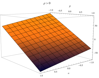
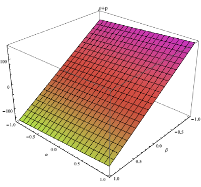
Figure 1: Plot of WEC for model 1 as in Eq.(24), the left plot shows $\rho$ while the right plot shows $\rho+p$ with respect to $\alpha$ and $\beta$

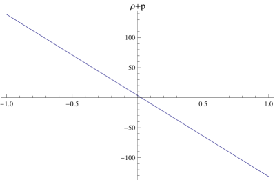
Figure 2: Contour plots of WEC for model 1, the left plot shows $\rho$ while the right plot shows $\rho+p$ versus $\beta$.

4.2 Model 2

Next, we consider an interesting higher derivative model of the type

$$f(R,\Box R)=R+\alpha{R^{2}}\left({1+\gamma R}\right)+\beta R\Box R,$$ (25)

where $\alpha,~{}\beta$ and $\gamma$ belong to set of real numbers. Equations (21) and (22), after using Eqs.(23) and (25) with some manipulation, give rise to

$$\rho =3{H^{2}}(1-2q-6\alpha{H^{2}}(-3+2j-6q+3{q^{2}})+2\beta{H^{3}}(12-l+2\left({10+7j}\right)q$$

$$+6{q^{2}}+s)+6{H^{4}}(-11\beta-66\alpha\gamma+\beta{j^{2}}-\beta l+23\beta q+27\beta{q^{2}}+90\alpha\gamma{q^{2}}+8\beta$$

$$\times{q^{3}}-24\alpha\gamma{q^{3}}+j\left({3\beta+36\alpha\gamma+5\beta q-36\alpha\gamma q}\right)+\beta qs)),$$

while, it follows from the sum of energy density and pressure that

$$\rho+p =2{H^{2}}(-1-q+6\alpha{H^{2}}\left({13+j+16q+2{q^{2}}+s}\right)+3\beta{H^{3}}(12-l+2$$

$$\times\left({10+7j}\right)q+6{q^{2}}+s)+3{H^{4}}(-83\beta-576\alpha\gamma+4\left({\beta-9\alpha\gamma}\right){j^{2}}-9\beta l$$

$$-24\beta q-288\alpha\gamma q+45\beta{q^{2}}+432\alpha\gamma{q^{2}}+24\beta{q^{3}}+108\alpha\gamma{q^{3}}+j\{3(\beta+36$$

$$\times\alpha\gamma)+(113\beta+108\alpha\gamma)q\}-4\beta s-36\alpha\gamma s+2\beta qs+36\alpha\gamma qs)).$$

The ECs corresponding to the cosmic FRW model mediated by the above mentioned model can be obtained through various numerical graphs. We have explored these conditions and found that the inequalities of WEC can be fulfilled by the perfect FRW metric under the following parametric zonal values of spacetime. The validity region ($\rho>0$) imposes that for $\beta$ to be in $[-1,1]$ makes the values of $\gamma$ and $\alpha$ to be the open intervals $(-0.4,-1)$ and $(-0.4,0.5)$, respectively. One can also find the regions where $\rho>0$ by considering $\alpha$ belonging to $[-1,1]$ with negative and positive values of $\beta$ and $\gamma$, respectively. Similarly, the validity regions for $\rho+p>0$ have been investigated in Figure 3. It is observed that for all choices of $\beta$ from $[-1,1]$ with $\gamma\in(-1,-0.7)$ and $\alpha\in(-0.6,1)$ give $\rho+p>0$. Another region has been seen for the positivity of $\rho+p$ under which the tetrad of $\beta,~{}\gamma$ and $\alpha$ should be from $[-1,1],~{}\gamma\in(0.6,1)$ and $\alpha\in(-1,0.7)$, respectively. We have shown graphically the energy condition, as shown in Figure 3, in which the left plot is for $\rho>0$ while the right plot is for $\rho+p>0$.

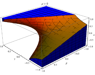
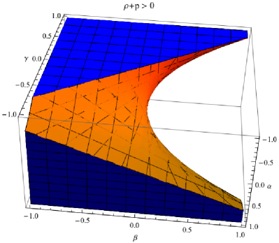
Figure 3: Plot of WEC for model 2 as in Eq.(25), the left plot shows $\rho>0$ while the right plot represents $\rho+p>0$ with respect to $\alpha$, $\beta$ and $\gamma$.

Model 2 could be treated as another modification of Starobinsky inflationary model with an addition of higher derivative term ($\Box$ R). In view of its compatibility with latest Planck data, the parameter $\alpha$ restricts the parameter $\beta$ and $\gamma$. We have explored that for which values of $\alpha,~{}\beta$ and $\gamma$ the WEC holds. These are shown in the Figure 3. We have plotted the 3D graph to find the range of $\gamma$ for which the WEC holds corresponding to $\beta=-1$. Consequently, we have verified the range of $\beta$ for particular values of $\alpha$ and $\gamma$. These results are indicated in Figures 4 and 5.

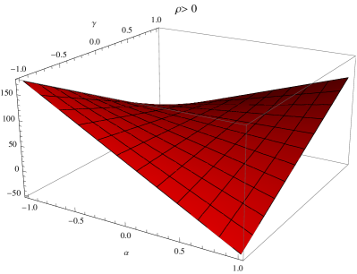
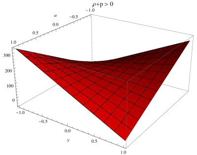
Figure 4: Plot of WEC for model 2 with respect to $\alpha$ and $\gamma$.

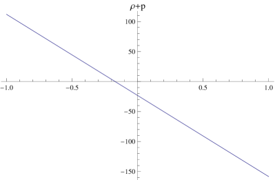
Figure 5: Plots of WEC for model 2 versus $\beta$ for particular values of $\alpha$ and $\gamma$.

4.3 Model 3

Now, we consider modified curvature terms of the form

$$f=R+\alpha R\left[{exp(-R/\gamma)-1}\right]+\beta R\Box R.$$ (26)

This model could consistent DE results, which was introduced (with $\beta=0$) in [72]. Furthermore, one can study details about similar models on some $f(G)$ gravity which was first introduced in [73]. By making use of expressions of snap, jerk and cackle along with Eqs.(21) and (22) , we get the following form of the equations of motion

$$\rho =\frac{3H^{2}}{{{\gamma^{2}}}}{{\rm{e}}^{-\frac{{6{H^{2}}\left({1+q}\right)}}{\gamma}}}\left[\left({{{\rm{e}}^{\frac{{6{H^{2}}\left({1+q}\right)}}{\gamma}}}\left({-1+\alpha}\right)-{{\rm{e}}^{\frac{{12{H^{2}}}}{\gamma}}}\alpha}\right){\gamma^{2}}\left({-1+2q}\right)+6{{\rm{e}}^{\frac{{12{H^{2}}}}{\gamma}}}\alpha\right.$$

$$\times\left.\gamma{H^{2}}(-4+2j-3q+{q^{2}})+2{{\rm{e}}^{\frac{{6{H^{2}}\left({1+q}\right)}}{\gamma}}}\beta{\gamma^{2}}{H^{3}}(12-l+2\left({10+7j}\right)q+6{q^{2}}\right.$$

$$\left.+s)+6{{\rm{e}}^{\frac{{6{H^{2}}}}{\gamma}}}{H^{4}}(-12{{\rm{e}}^{\frac{{6{H^{2}}}}{\gamma}}}\alpha-11{{\rm{e}}^{\frac{{6{H^{2}}q}}{\gamma}}}\beta{\gamma^{2}}+{{\rm{e}}^{\frac{{6{H^{2}}q}}{\gamma}}}\beta{\gamma^{2}}{j^{2}}-{{\rm{e}}^{\frac{{6{H^{2}}q}}{\gamma}}}\beta{\gamma^{2}}l+6{{\rm{e}}^{\frac{{6{H^{2}}}}{\gamma}}}\right.$$

$$\times\left.\alpha q+23{{\rm{e}}^{\frac{{6{H^{2}}q}}{\gamma}}}\beta{\gamma^{2}}q+6{{\rm{e}}^{\frac{{6{H^{2}}}}{\gamma}}}\alpha{q^{2}}+27{{\rm{e}}^{\frac{{6{H^{2}}q}}{\gamma}}}\beta{\gamma^{2}}{q^{2}}+8{{\rm{e}}^{\frac{{6{H^{2}}q}}{\gamma}}}\beta{\gamma^{2}}{q^{3}}+j(6{{\rm{e}}^{\frac{{6{H^{2}}}}{\gamma}}}\alpha\right.$$

$$\left.+3{{\rm{e}}^{\frac{{6{H^{2}}q}}{\gamma}}}\beta{\gamma^{2}}+\left({-6{{\rm{e}}^{\frac{{6{H^{2}}}}{\gamma}}}\alpha+5{{\rm{e}}^{\frac{{6{H^{2}}q}}{\gamma}}}\beta{\gamma^{2}}}\right)q)+{{\rm{e}}^{\frac{{6{H^{2}}q}}{\gamma}}}\beta{\gamma^{2}}qs)\right],$$

and

$$\rho+p =\frac{1}{{{\gamma^{3}}}}2{{\rm{e}}^{-\frac{{6{H^{2}}\left({1+q}\right)}}{\gamma}}}{H^{2}}\left[\left({{{\rm{e}}^{\frac{{6{H^{2}}\left({1+q}\right)}}{\gamma}}}\left({-1+\alpha}\right)-{{\rm{e}}^{\frac{{12{H^{2}}}}{\gamma}}}\alpha}\right){\gamma^{3}}\left({1+q}\right)+108{{\rm{e}}^{\frac{{12{H^{2}}}}{\gamma}}}\right.$$

$$\times\left.\alpha{H^{6}}\left({-1+q}\right){\left({2-j+q}\right)^{2}}-6{{\rm{e}}^{\frac{{12{H^{2}}}}{\gamma}}}\alpha{\gamma^{2}}{H^{2}}(12+j+16q+3{q^{2}}+s)+3\right.$$

$$\times\left.{{\rm{e}}^{\frac{{6{H^{2}}\left({1+q}\right)}}{\gamma}}}\beta{\gamma^{3}}{H^{3}}(12-l+2\left({10+7j}\right)q+6{q^{2}}+s)+3\gamma{H^{4}}\left\{\left(-18{{\rm{e}}^{\frac{{12{H^{2}}}}{\gamma}}}\alpha\right.\right.\right.$$

$$\left.\left.\left.+4{{\rm{e}}^{\frac{{6{H^{2}}\left({1+q}\right)}}{\gamma}}}\beta{\gamma^{2}}\right){j^{2}}+j\left(66{{\rm{e}}^{\frac{{12{H^{2}}}}{\gamma}}}\alpha+3{{\rm{e}}^{\frac{{6{H^{2}}\left({1+q}\right)}}{\gamma}}}\beta{\gamma^{2}}+\left(42{{\rm{e}}^{\frac{{12{H^{2}}}}{\gamma}}}\alpha+113\right.\right.\right.\right.$$

$$\left.\left.\left.\left.\times{{\rm{e}}^{\frac{{6{H^{2}}\left({1+q}\right)}}{\gamma}}}\beta{\gamma^{2}}\right)q\right)+{{\rm{e}}^{\frac{{6{H^{2}}}}{\gamma}}}\left[-138{{\rm{e}}^{\frac{{6{H^{2}}}}{\gamma}}}\alpha-83{{\rm{e}}^{\frac{{6{H^{2}}q}}{\gamma}}}\beta{\gamma^{2}}-9{{\rm{e}}^{\frac{{6{H^{2}}q}}{\gamma}}}\beta{\gamma^{2}}l+9\right.\right.\right.$$

$$\times\left.\left.\left.(6{{\rm{e}}^{\frac{{6{H^{2}}}}{\gamma}}}\alpha+5{{\rm{e}}^{\frac{{6{H^{2}}q}}{\gamma}}}\beta{\gamma^{2}}){q^{2}}+24\left({{{\rm{e}}^{\frac{{6{H^{2}}}}{\gamma}}}\alpha+{{\rm{e}}^{\frac{{6{H^{2}}q}}{\gamma}}}\beta{\gamma^{2}}}\right){q^{3}}-6{{\rm{e}}^{\frac{{6{H^{2}}}}{\gamma}}}\alpha s-4\right.\right.\right.$$

$$\times\left.\left.\left.{{\rm{e}}^{\frac{{6{H^{2}}q}}{\gamma}}}\beta{\gamma^{2}}s+2q\left({3{{\rm{e}}^{\frac{{6{H^{2}}}}{\gamma}}}\alpha s-51{{\rm{e}}^{\frac{{6{H^{2}}}}{\gamma}}}\alpha-12{{\rm{e}}^{\frac{{6{H^{2}}q}}{\gamma}}}\beta{\gamma^{2}}+{{\rm{e}}^{\frac{{6{H^{2}}q}}{\gamma}}}\beta{\gamma^{2}}s}\right)\right\}\right]\right].$$ (27)

We want to check the validity regimes for WEC in this context. Through graphs, the validity regions for $\rho>0$ impose the following constrains on the parameters of $f(R,\Box R,T)$ model
(i) For all $\alpha\in[-1,1]$, $\beta$ and $\gamma$ depend on each other, like $\beta<0$ while $\gamma>2$.
(ii) For all $\beta\in[-1,1]$, $\alpha$ and $\gamma$ depend on each other, e.g $\alpha<0$ then $\gamma<2$.
Similarly, the condition $\rho+p>0$ provides the following limitations on $\alpha,~{}\beta$ and $\gamma$
(i) For all $\alpha\in[-1,1]$, $\beta$ and $\gamma$ depend on each other, like $\beta<0$ while $\gamma>2.1$.
(ii) For all $\beta\in[-1,1]$, $\alpha$ and $\gamma$ depend on each other, e.g $\alpha<0$ then $\gamma<2.1$.
We have shown graphically the viable zones of WEC in Figure 6. It can be noticed that the left plot of the Figure (6) describes $\rho>0$, its right plot provides zones for $\rho+p>0$.

Modified gravity theories has a significant role in various forms in the discussion of the universe’s evolution. It is worth mentioning that a number of viable $f(R)$ gravity models leading to a unified description of inflation with late time cosmic acceleration have been identified in literature. Elizalde et al. [69] proposed a reasonably simple and a viable version of $f(R)$ gravity via an exponential modified gravity model which explains in a unified way both the late time acceleration and early time inflation and successfully fulfils the cosmological bounds as well as compatible with the known local tests. This exponential gravity is indeed free from any kind of finite time future singularity and exhibit various interesting properties. They also claimed that slight generalization to this theory may yield other well-behaved non-singular stable class of exponential gravity models with similar physical predictions. Bamba et al. [70] presented a detailed analysis on the evolution history of the growth index of matter density perturbation as well as the future evolution of the universe via the exponential gravity model. They exhibited the numerical analysis of inflation via couple of viable exponential gravity models. They also investigated the behavior of extra correction ingredients in the exponential gravity model to examine the cosmic acceleration and inflation.

Odintsov et al. [71] provided various interesting properties of the reheating regime via the logarithmic correction in the $R^{2}$ gravity model as this provide a unification of late and early acceleration era. They also discussed the possibility to explore observational indices compatible with the latest Planck data. We have considered an exponential gravity model to explore the viability regions for WEC. In this case, we have plotted 3D the results of WEC with negative values of $\beta$ to explore the range of $\gamma$ where WEC holds (shown in Figure 6). Further, we have plotted the WEC for the extracted value of $\gamma$ and $\beta$ to examine the viability regions for WEC. All this analysis have been shown via plots in Figures 7 and 8.

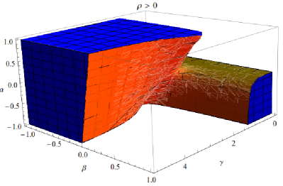
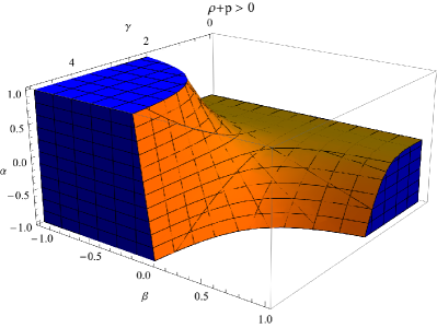
Figure 6: Plot of WEC for model 3 as in Eq.(26), the left plot indicates $\rho>0$ while the right plot shows $\rho+p>0$ with respect to $\alpha$, $\beta$ and $\gamma$.

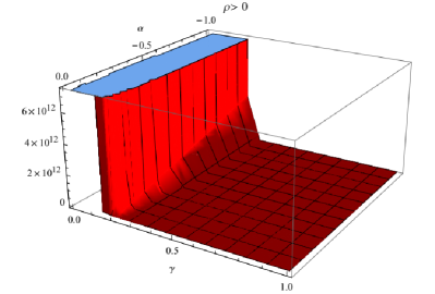
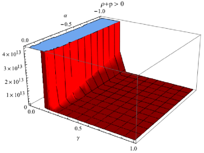
Figure 7: Plot of WEC for model 3, the left plot indicates $\rho>0$ while the right plot shows $\rho+p>0$ with respect to $\alpha$ and $\gamma$.

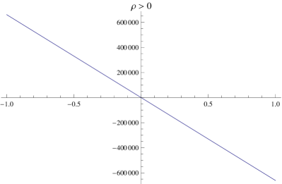
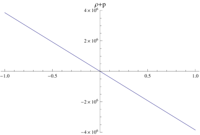
Figure 8: Plot of WEC for model 3, the left plot indicates $\rho>0$ while the right plot shows $\rho+p>0$ for particular values of $\beta$ and $\gamma$ with respect to $\alpha$.

5 Summary

The existence of a generic higher-derivative curvature quantities term in the extended version of EH action could help to provide some dynamical features of canonical Einstein gravity (after using conformal transformations) along with finite scalar degrees of freedom. From these, one can notice that few fields mediated by scalar variables are propagating with proper mathematical and physical grounds. The present paper is devoted to investigate the impact of $f(R,\Box R,T)$ extra curvature terms in the modeling of realistic cosmic ideal fluid models. The Lagrangian of $f(R,\Box R,T)$ gravity could be regarded as more comprehensive in its meaning that suggests that various functional formulations of $f$ could be introduced. Due to the arrival of a wide variety of these functions, the need of the hour is to constrain such gravitational theory on mathematical as well as physical backgrounds. The validity of this gravitational model could be dealt by analyzing the stability constraints against local perturbations which is widely known as Dolgov-Kawasaki instability.

This work is devoted to develop some conditions on comprehensive as well as particular configurations of $f(R,\Box R,T)$ models by investigating the applicability of respective ECs. We have used expressions for NEC and SEC that could be calculated after using the notable Raychaudhuri equation with an environment of the attractive nature of gravity. This gives rise to even more generic computations of results as compared to $f(R)$ and $f(R,T)$ gravitational models. Furthermore, these expressions are found to be equivalent to that determined by $\rho+3p\geq 0$ and $\rho+p\geq 0$ after using particular mathematical transformations on mater variables, i.e., $p\rightarrow p_{eff}$ and $\rho\rightarrow\rho_{eff}$ , respectively. In a similar fashion, one can utilize the corresponding constraints for WEC and DEC by transforming the counterpart matter quantities in GR for $f(R,\Box R,T)$ energy-momentum tensor.

In order to evaluate the viability constraints for $f(R,\Box R,T)$ gravity, we have considered three particular cosmic models specifically, $f(R,\Box R)=R+\alpha{R^{2}}+\beta R\Box R,~{}f(R,\Box R)=R+\alpha{R^{2}}\left({1+\gamma R}\right)+\beta R\Box R$ and $f(R,\Box R)=R+\alpha R\left[{exp(-R/\gamma)-1}\right]+\beta R\Box R$. We have used the expressions of snap, jerk and crackle that are being evaluated through Hubble parameter. It is shown that WEC for these models depends on the particular choices of $\alpha,~{}\beta$ and $\gamma$. The ECs are valid in the first model, once we set $\beta<0$. The plot has been shown in order to mention the viability bounds of WEC within the background of $f(R,\Box R)=R+\alpha{R^{2}}+\beta R\Box R$ in Figure 1. For the case of second model, i.e., $f(R,\Box R)=R+\alpha{R^{2}}\left({1+\gamma R}\right)+\beta R\Box R$, we proceed our examination to obtain validity regions of WEC. We found that zone satisfying $\rho+p>0$ constraint for the FRW perfect model can be obtained by keeping $\beta$ to be in $[-1,1]$ along with $-1<\gamma<-0.7$ and $-0.6<\alpha<1$. Furthermore, the validity regions for $\rho+p>0$ can be found by taking any choice of $\beta$ from $[-1,1]$ together with $\gamma\in(0.6,1)$ and $\alpha\in(-1,0.7)$. The viability bounds on the formulations of second models for $\rho>0$ are found as $\beta\in[-1,1]$ along with $\gamma\in(-1,-0.4)$ and $\alpha\in(-0.4,0.5)$. Figure 3 also indicates that conditions on the parameters of $f$ model for the applicability of $\rho>0$, are $\alpha\in[-1,1],~{}\beta<0$ and $\gamma>0$. The EC $\rho>0$ for $f(R,\Box R)=R+\alpha R\left[{\exp(-R/\gamma)-1}\right]+\beta R\Box R$ is met, if we take $\alpha\in[-1,1]$ with negative choice of $\beta$ and $\gamma$ to be greater than 2. Furthermore, to keep $\beta\in[-1,1],~{}\alpha<0$ and $\gamma<2$, the viability zones for $\rho>0$ can be found as shown in Figure 6. We further found that one of the conditions of WEC, $\rho+p>0$, is valid under the parametric limits $\alpha\in[-1,1]$ along with $\beta<0$ and $\gamma>2.1$. Also, the region governed by $\beta\in[-1,1],~{}\alpha<0$ and $\gamma<2.1$ provides the viability bounds for $\rho+p>0$.

The terminology of “modified gravity” has received great attention that depicts gravitational interactions, differ from the most established theory of general relativity. It is pertinent to mention here that the investigation for the well-consistent $f(R,\Box R,T)$ gravity models can be extended for the notion that there could exist some convenient usual complex fluid configurations corresponding to FLRW geometry. Then, the perspective research may give rise to some substantial qualitative consequences in comparison with the discussion of pure gravity. It will be executed elsewhere.

References

- [1] P. A. R. Ade et al. [Planck Collaboration], Astron. Astrophys. 571, A1 (2014).
- [2] P. A. R. Ade et al. [Planck Collaboration], Astron. Astrophys. 594, A13 (2016) [arXiv:1502.01589 [astro-ph.CO]].
- [3] P. A. R. Ade et al. [Planck Collaboration], Astron. Astrophys. 594, A20 (2016) [arXiv:1502.02114 [astro-ph.CO]].
- [4] P. A. R. Ade et al. [BICEP2 Collaboration], Phys. Rev. Lett. 112, 241101 (2014) [arXiv:1403.3985 [astro-ph.CO]].
- [5] P. A. R. Ade et al. [BICEP2 and Planck Collaborations], Phys. Rev. Lett. 114, 101301 (2015) [arXiv:1502.00612 [astro-ph.CO]].
- [6] P. A. R. Ade et al. [BICEP2 and Keck Array Collaborations], arXiv:1510.09217 [astro-ph.CO].
- [7] E. Komatsu et al. [WMAP Collaboration], Astrophys. J. Suppl. 192, 18 (2011) [arXiv:1001.4538 [astro-ph.CO]].
- [8] G. Hinshaw et al. [WMAP Collaboration], Astrophys. J. Suppl. 208, 19 (2013) [arXiv:1212.5226 [astro-ph.CO]].
- [9] A. Qadir, H. W. Lee, and K. Y. Kim, Int. J. Mod. Phys. D 26, 1741001 (2017).
- [10] A. Joyce, B. Jain, J. Khoury and M. Trodden, Phys. Rept. 568, 1 (2015) [arXiv:1407.0059 [astro-ph.CO]].
- [11] S. Capozziello and V. Faraoni, Beyond Einstein Gravity (Springer, Dordrecht, 2010).
- [12] S. Capozziello and M. De Laurentis, Phys. Rept. 509, 167 (2011) [arXiv:1108.6266 [gr-qc]].
- [13] K. Bamba, Capozziello, S., Nojiri, S. and Odintsov, S. D.: Astrophys. Space Sci. 342, 155 (2012) [arXiv:1205.3421 [gr-qc]].
- [14] K. Koyama, Rep. Prog. Phys. 79, 046902 (2016) [arXiv:1504.04623 [astro-ph.CO]].
- [15] Á. de la Cruz-Dombriz and D. Sáez-Gómez, Entropy 14, 1717 (2012) [arXiv:1207.2663 [gr-qc]].
- [16] K. Bamba, S. Nojiri and S. D. Odintsov arXiv:1302.4831 [gr-qc].
- [17] K. Bamba and S. D. Odintsov, arXiv:1402.7114 [hep-th]. Symmetry 7, 220 (2015) [arXiv:1503.00442 [hep-th]].
- [18] Z. Yousaf, K. Bamba and M. Z. Bhatti, Phys. Rev. D 93, 064059 (2016) [arXiv1603.03175 [gr-qc]].
- [19] Z. Yousaf, K. Bamba and M. Z. Bhatti, Phys. Rev. D 93, 124048 (2016) [arXiv:1606.00147 [gr-qc]].
- [20] S. Nojiri and S. D. Odintsov eConf C 0602061, 06 (2006); Int. J. Geom. Meth. Mod. Phys. 4, 115 (2007) [hep-th/0601213].
- [21] S. Nojiri and S. D. Odintsov arXiv:0801.4843 [astro-ph] (2008).
- [22] S. Nojiri and S. D. Odintsov arXiv:0807.0685 [hep-th] (2008).
- [23] T. P. Sotiriou and V. Faraoni, Rev. Mod. Phys. 82, 451 (2010) [arXiv:0805.1726 [gr-qc]].
- [24] S. Capozziello and M. Francaviglia, Gen. Relativ. Gravit. 40, 357 (2008).
- [25] S. Nojiri and S. D. Odintsov, Phys. Rev D 68, 123512 (2003).
- [26] S. Nojiri, S. D. Odintsov and V. K. Oikonomou, Phys. Rept. 692, 1 (2017) [arXiv:1705.11098 [gr-qc]].
- [27] M. Z. Bhatti, Eur. Phys. J. Plus 131, 428 (2016); Z. Yousaf, Eur. Phys. J. Plus 132, 71 (2017).
- [28] M. Sharif and Z. Yousaf, Z.: Astrophys. Space Sci. 355, 317 (2015); M. Z. Bhatti and Z. Yousaf, Int. J. Mod. Phys. D 26, 1750029 (2017); ibid. Int. J. Mod. Phys. D 26, 1750045 (2017); M. Z. Bhatti and Z. Yousaf, Eur. Phys. J. C 76, 219 (2016) [arXiv1604.01395 [gr-qc]].
- [29] T. Harko, F. S. N. Lobo, S. Nojiri and S. D. Odintsov, Phys. Rev. D 84, 024020 (2011); Z. Yousaf and M. Z. Bhatti, Eur. Phys. J. C 76, 267 (2016) [arXiv:1604.06271 [physics.gen-ph]]; M. Sharif and Z. Yousaf, Astrophys. Space Sci. 354, 471 (2014); Yousaf, Z., Bamba, K. and Bhatti, M. Z.: Phys. Rev. D 95, 024024 (2017) [arXiv:1701.03067 [gr-qc]].
- [30] S. D. Odintsov and D. Sáez-Gómez, Phys. Lett. B, 725, 437 (2013); Z. Haghani, T. Harko, F. S. N. Lobo, H. R. Sepangi and S. Shahidi, Phys. Rev. D, 88, 044023 (2013); I. Ayuso, J. B. Jiménez and Á de la Cruz-Dombriz, Phys. Rev. D, 91, 104003 (2015); Z. Yousaf, M. Z. Bhatti and U. Farwa, Class. Quantum Grav. 34, 145002 (2017).
- [31] A. S. Eddington, : The Mathematical Theory of Relativity. (Cambridge University Press, 1923); H. J. Schmidt, Int. J. Geom. Meth. Phys. 4, 209 (2007).
- [32] C. Lanczos, Zeit. Phys. 73, 147 (1932); E. Schrödinger, Space-Time Structure, (Cambridge University Press, 1950); H. Buchdhal, Quart. J. Math. 19, 150 (1948); Proc. Nat. Acad. Sci. 34, 66 (1948); Acta Mathematica 85, 63 (1951); J. London Math. Soc. 26, 139 (1951); Mon. Not. R. Astron. Soc. 150, 1 (1970); J. Phys. A 11, 871 (1978); Int. J. Theor. Phys. 17, 149 (1978).
- [33] R. Utiyama and B. DeWitt, J. Math. Phys. 3, 608 (1962); A. Strominger, Phys. Rev. D 30, 2257 (1984).
- [34] T. Harko, F. S. N. Lobo, S. Nojiri and S. D. Odintsov, Phys. Rev. D 84, 024020 (2011).
- [35] M. J. S. Houndjo, M. E. Rodrigues, N. S. Mazhari, D. Momeni and R. Myrzakulov, Int. J. Mod. Phys. D 26, 1750024 (2017).
- [36] A. Hindawi, B. A. Ovrut and D. Waldram, Phys. Rev. D 53, 5597 (1996) [hepth/ 9509147]
- [37] H. -J. Schmidt, Class. Quantum Grav. 7, 10231031 (1990); D. Wands, Class. Quantum Grav. 11, 269279 (1994).
- [38] M. Sharif and Z. Yousaf, J. Cosmol. Astropart. Phys. 06, 019 (2014); Astrophys. Space Sci. 357, 49 (2015); ibid. 355, 317 (2015); Gen. Relativ. Gravit. 47, 48 (2015); Can. J. Phys. 93, 905 (2015); Eur. Phys. J. C 75, 58 (2015); ibid. 75, 194 (2015) [arXiv:1504.04367v1 [gr-qc]].
- [39] M. Sharif and H. R. Kausar, Phys. Lett. B 697, 1 (2011); ibid. Astrophys. Space Sci. 332, 463 (2011).
- [40] S. W. Hawking and G. F. R. Ellis, The Large Scale Structure of Spacetime, Cambridge University Press, Cambridge (1973).
- [41] R. M. Wald, General Relativity, University of Chicago Press, Chicago (1984).
- [42] S. Carroll, Spacetime and Geometry: an Introduction to General Relativity, Addison-Wesley, New York (2004).
- [43] M. Visser, Phys. Rev D 56, 12 (1997).
- [44] J. Santos, J. S. Alcaniz and M. J. Rebouças, Phys. Rev. D 74, 067301 (2006) [arXiv:astro-ph/0608031].
- [45] J. Santos, J. S. Alcaniz, M. J. Rebouças and F. C. Carvalho, Phys. Rev. D 76, 083513 (2007) [arXiv:0708.0411 [astro-ph]].
- [46] J. Santos, J. S. Alcaniz, N. Pires and M. J. Rebouças, Phys. Rev. D 75, 083523 (2007) [arXiv:astro-ph/0702728].
- [47] O. Bertolami and M. C. Sequeira, Phys. Rev. D 79, 104010 (2009).
- [48] K. Atazadeh, A. Khaleghi, H. R. Sepangi and Y. Tavakoli, Int. J. Mod. Phys. D 18, 1101 (2009).
- [49] A. A. Sen and R. J. Scherrer, Phys. Lett. B 659, 457 (2008) [arXiv:astro-ph/0703416].
- [50] S. Nojiri, S. D. Odintsov and P. V. Tretyakov, Prog. Theor. Phys. Suppl. 172, 81 (2008).
- [51] K. Bamba, M. Ilyas, M. Z. Bhatti and Z. Yousaf, Gen. Relativ. Gravit. 49, 112 (2017) [arXiv:1707.07386 [gr-qc]].
- [52] Z. Yousaf, Eur. Phys. J. Plus 132, 276 (2017).
- [53] A. Banijamali, B. Fazlpour and M. R. Setare, Astrophys. Space Sci. 338 327 (2012) [arXiv:1111.3878 [physics.gen-ph]].
- [54] J. Sadeghi, A. Banijamali and H. Vaez, Int. J. Theor. Phys. 51, 2888 (2012); S. -Y. Zhou, E. J. Copeland and P. M. Saffin, J. Cosmool. Astropart. Phys. 7, 009 (2009) [arXiv:0903.4610 [gr-qc]].
- [55] K. Atazadeh and F. Darabi, Gen. Relativ. Gravit. 46, 1664 (2014) [arXiv:1302.0466 [gr-qc]].
- [56] A. Övgün and0 I. Sakalli, Theor. Math. Phys. 190, 120 (2017) [arXiv:1507.03949 [gr-qc]].
- [57] I. Sakalli and A. Övgün, Astrophys. Space Sci. 359, 32 (2015) [arXiv:1506.00599 [gr-qc]].
- [58] M. Halilsoy, A. Övgün and S. H. Mazharimousavi, Eur. Phys. J. C 74, 2796 (2014) [arXiv:1312.6665 [gr-qc]].
- [59] C. Bambi, A. Cardenas-Avendano, G. J. Olmo and D. Rubiera-Garcia, Phys. Rev. D 93, 064016 (2016).
- [60] P. K. Sahoo, P. H. R. S. Moraes and P. Sahoo, arXiv:1709.07774 [gr-qc].
- [61] Z. Yousaf, M. Ilyas and M. Z. Bhatti, Eur. Phys. J. Plus 132, 268 (2017).
- [62] M. Sharif and A. Ikram, Phys. Dark Universe 17, 1 (2017); Int. J. Mod. Phys. D 26, 1750084 (2017); arXiv:1707.05162; M. Sharif and M. Z. Bhatti, Astrophys. Space Sci. 347, 337 (2013).
- [63] A. A. Starobinsky, Phys. Lett. B 91, 99 (1980).
- [64] S. Capozziello, S. Nojiri and S. D. Odintsov, Phys. Lett. B 632, 597 (2006); A. Borowiec, W. Godłowski and M. Szydłowski, Int. J. Geom. Meth. Mod. Phys. 4, 183 (2007); S. Capozziello, V. F. Cardone and A. Troisi, Mon. Not. R. Astron. Soc. 375, 1423 (2007); A. Kelleher, arXiv:1309.3523.
- [65] J. A. R. Cembranos, Phys. Rev. Lett. 102, 141301 (2009); J. Phys. Conf. Ser. 315, 012004 (2011).
- [66] J. A. R. Cembranos, A. D. L. Cruz-Dombriz and B. M. Núñez, J. Cosmol. Astropart. Phys. 04, 021 (2012).
- [67] M. Ozkan, Y. Pang and S. Tsujikawa, Phys. Rev. D 92, 023530 (2015).
- [68] S.D. Odintsov and V.K. Oikonomou Phys. Rev. D 92, 124024 (2015).
- [69] E. Elizalde, S. Nojiri, S. D. Odintsov, L. Sebastiani and S. Zerbini, Phys. Rev. D 83, 086006 (2011).
- [70] K. Bamba, A. Lopez-Revelles, R. Myrzakulov, S. D. Odintsov and L. Sebastiani, Class. Quantum Grav. 30, 015008 (2013).
- [71] S. D. Odintsov, V. K. Oikonomou and L. Sebastiani, Nucl. Phys. B 923, 608 (2017).
- [72] G. Cognola, E. Elizalde, S. Nojiri, S.D. Odintsov, L. Sebastiani and S. Zerbini, Phys. Rev. D 77, 046009 (2008) [arXiv:0712.4017 [hep-th]].
- [73] S. Nojiri and S. D. Odintsov, Phys. Lett. B 631, 1 (2005) [arXiv:hep-th/0508049].