N-Gram Graph: Simple Unsupervised Representation for Graphs, with Applications to Molecules

Abstract

Machine learning techniques have recently been adopted in various applications in medicine, biology, chemistry, and material engineering. An important task is to predict the properties of molecules, which serves as the main subroutine in many downstream applications such as virtual screening and drug design. Despite the increasing interest, the key challenge is to construct proper representations of molecules for learning algorithms. This paper introduces the N-gram graph, a simple unsupervised representation for molecules. The method first embeds the vertices in the molecule graph. It then constructs a compact representation for the graph by assembling the vertex embeddings in short walks in the graph, which we show is equivalent to a simple graph neural network that needs no training. The representations can thus be efficiently computed and then used with supervised learning methods for prediction. Experiments on 60 tasks from 10 benchmark datasets demonstrate its advantages over both popular graph neural networks and traditional representation methods. This is complemented by theoretical analysis showing its strong representation and prediction power.

1 Introduction

Increasingly, sophisticated machine learning methods have been used in non-traditional application domains like medicine, biology, chemistry, and material engineering [14, 11, 16, 9]. This paper focuses on a prototypical task of predicting properties of molecules. A motivating example is virtual screening for drug discovery. Traditional physical screening for drug discovery (i.e., selecting molecules based on properties tested via physical experiments) is typically accurate and valid, but also very costly and slow. In contrast, virtual screening (i.e., selecting molecules based on predicted properties via machine learning methods) can be done in minutes for predicting millions of molecules. Therefore, it can be a good filtering step before the physical experiments, to help accelerate the drug discovery process and significantly reduce resource requirements. The benefits gained then depend on the prediction performance of the learning algorithms.

A key challenge is that raw data in these applications typically are not directly well-handled by existing learning algorithms and thus suitable representations need to be constructed carefully. Unlike image or text data where machine learning (in particular deep learning) has led to significant achievements, the most common raw inputs in molecule property prediction problems provide only highly abstract representations of the chemicals (i.e., graphs on atoms with atom attributes).

To address the challenge, various representation methods have been proposed, mainly in two categories. The first category is chemical fingerprints, the most widely used feature representations in aforementioned domains. The prototype is the Morgan fingerprints  [42] (see Figure S1 for an example). The second category is graph neural networks (GNN) [25, 2, 33, 47, 26, 58]. They view the molecules as graphs with attributes, and build a computational network tailored to the graph structure that constructs a embedding vector for the input molecule and feed into a predictor (classifier or regression model). The network is trained end-to-end on labeled data, learning the embedding and the predictor at the same time.

These different representation methods have their own advantages and disadvantages. The fingerprints are simple and efficient to calculate. They are also unsupervised and thus each molecule can be computed once and used by different machine learning methods for different tasks. Graph neural networks in principle are more powerful: they can capture comprehensive information for molecules, including the skeleton structure, conformational information, and atom properties; they are trained end-to-end, potentially resulting in better representations for prediction. On the other hand, they need to be trained via supervised learning with sufficient labeled data, and for a new task the representation needs to retrained. Their training is also highly non-trivial and can be computationally expensive. So a natural question comes up: can we combine the benefits by designing a simple and efficient unsupervised representation method with great prediction performance?

To achieve this, this paper introduces an unsupervised representation method called N-gram graph. It views the molecules as graphs and the atoms as vertices with attributes. It first embeds the vertices by exploiting their special attribute structure. Then, it enumerates n-grams in the graph where an n-gram refers to a walk of length $n$, and constructs the embedding for each n-gram by assembling the embeddings of its vertices. The final representation is constructed based on the embeddings of all its n-grams. We show that the graph embedding step can also be formulated as a simple graph neural network that has no parameters and thus requires no training. The approach is efficient, produces compact representations, and enjoys strong representation and prediction power shown by our theoretical analysis. Experiments on 60 tasks from 10 benchmark datasets show that it gets overall better performance than both classic representation methods and several recent popular graph neural networks.

Related Work.

We briefly describe the most related ones here due to space limitation and include a more complete review in Appendix A. Firstly, chemical fingerprints have long been used to represent molecules, including the classic Morgan fingerprints [42]. They have recently been used with deep learning models [38, 52, 37, 31, 27, 34]. Secondly, graph neural networks are recent deep learning models designed specifically for data with graph structure, such as social networks and knowledge graphs. See Appendix B for some brief introduction and refer to the surveys [30, 61, 57] for more details. Since molecules can be viewed as structured graphs, various graph neural networks have been proposed for them. Popular ones include [2, 33, 47, 26, 58]. Finally, graph kernel methods can also be applied (e.g., [48, 49]). The implicit feature mapping induced by the kernel can be viewed as the representation for the input. The Weisfeiler-Lehman kernel [49] is particularly related due to its efficiency and theoretical backup. It is also similar in spirit to the Morgan fingerprints and closely related to the recent GIN graph neural network [58].

2 Preliminaries

Raw Molecule Data.

This work views a molecule as a graph, where each atom is a vertex and each bond is an edge. Suppose there are $m$ vertices in the graph, denoted as $i\in\{0,1,...,m-1\}$. Each vertex has useful attribute information, like the atom symbol and number of charges in the molecular graphs. These vertex attributes are encoded into a vertex attribute matrix $\mathcal{V}$ of size $m\times S$, where $S$ is the number of attributes. An example of the attributes for vertex $i$ is:

$$\mathcal{V}_{i,\cdot}=[\mathcal{V}_{i,0},\mathcal{V}_{i,1},\ldots,\mathcal{V}_{i,6},\mathcal{V}_{i,7}]$$

where $\mathcal{V}_{i,0}$ is the atom symbol, $\mathcal{V}_{i,1}$ counts the atom degree, $\mathcal{V}_{i,6}$ and $\mathcal{V}_{i,7}$ indicate if it is an acceptor or a donor. Details are listed in Appendix E. Note that the attributes typically have discrete values. The bonding information is encoded into the adjacency matrix $\mathcal{A}\in\{0,1\}^{m\times m}$, where $\mathcal{A}_{i,j}=1$ if and only if two vertices $i$ and $j$ are linked. We let $G=(\mathcal{V},\mathcal{A})$ denote a molecular graph. Sometimes there are additional types of information, like bonding types and pairwise atom distance in the 3D Euclidean space used by [33, 47, 26], which are beyond the scope of this work.

N-gram Approach.

In natural language processing (NLP), an n-gram refers to a consecutive sequence of words. For example, the 2-grams of the sentence “the dataset is large” are $\{$“the dataset”, “dataset is”, “is large”$\}$. The N-gram approach constructs a representation vector $c_{(n)}$ for the sentence, whose coordinates correspond to all n-grams and the value of a coordinate is the number of times the corresponding n-gram shows up in the sentence. Therefore, the dimension of an n-gram vector is $|V|^{n}$ for a vocabulary $V$, and the vector $c_{(1)}$ is just the count vector of the words in the sentence. The n-gram representation has been shown to be a strong baseline (e.g., [53]). One drawback is its high dimensionality, which can be alleviated by using word embeddings. Let $W$ be a matrix whose $i$-th column is the embedding of the $i$-th word. Then $f_{(1)}=Wc_{(1)}$ is just the sum of the word vectors in the sentence, which is in lower dimension and has also been shown to be a strong baseline (e.g., [55, 6]). In general, an n-gram can be embedded as the element-wise product of the word vectors in it. Summing up all n-gram embeddings gives the embedding vector $f_{(n)}$. This has been shown both theoretically and empirically to preserve good information for downstream learning tasks even using random word vectors (e.g., [3]).

3 N-gram Graph Representation

Our N-gram graph method consists of two steps: first embed the vertices, and then embed the graph based on the vertex embedding.

3.1 Vertex Embedding

Figure 1: The CBoW-like neural network $g$. Each small box represents one attribute, and the gray color represents the bit one since it is one-hot encoded. Each long box consists of $S$ attributes with length $K$. is the summation of all the embeddings of the neighbors of vertex $i$, where $W\in\mathbb{R}^{r\times K}$ is the vertex embedding matrix. is a fully-connected neural network, and the final predictions are the attributes of vertex $i$. s

The typical method to embed vertices in graphs is to view each vertex as one token and apply an analog of CBoW [41] or other word embedding methods (e.g., [28]). Here we propose our variant that utilizes the structure that each vertex has several attributes of discrete values. Recall that there are $S$ attributes; see Section 2. Suppose the $j$-th attribute takes values in a set of size $k_{j}$, and let $K=\sum_{j=0}^{S-1}k_{j}$. Let $h^{j}_{i}$ denote a one-hot vector encoding the $j$-th attribute of vertex $i$, and let $h_{i}\in\mathbb{R}^{K}$ be the concatenation $h_{i}=[h^{0}_{i};\ldots;h^{S-1}_{i}]$. Given an embedding dimension $r$, we would like to learn matrices $W^{j}\in\mathbb{R}^{r\times k_{j}}$ whose $\ell$-th column is an embedding vector for the $\ell$-th value of the $j$-th attribute. Once they are learned, we let $W\in\mathbb{R}^{r\times K}$ be the concatenation $W=[W^{0},W^{1},\ldots,W^{S-1}]$, and define the representation for vertex $i$ as

$$f_{i}=Wh_{i}.$$ (1)

Now it is sufficient to learn the vertex embedding matrix $W$. We use a CBoW-like pipeline; see Algorithm 1. The intuition is to make sure the attributes $h_{i}$ of a vertex $i$ can be predicted from the $h_{j}$’s in its neighborhood. Let $C_{i}$ denote the set of vertices linked to $i$. We will train a neural network $\hat{h}_{i}=g(\{h_{j}:j\in C_{i}\})$ so that its output matches $h_{i}$. As specified in Figure 1, the network $g$ first computes $\sum_{j\in C_{i}}Wh_{j}$ and then goes through a fully connected network with parameter $\theta$ to get $\hat{h}_{i}$. Given a dataset $\mathcal{S}=\{G_{j}=(\mathcal{V}_{j},\mathcal{A}_{j})\}$, the training is by minimizing the cross-entropy loss:

$$\min_{W,\theta}\sum_{G\in\mathcal{S}}\sum_{i\in G}\sum_{0\leq\ell<S}\text{cross-entropy}(h_{i}^{\ell},\hat{h}_{i}^{\ell}),\text{ subject to }[\hat{h}_{i}^{0};\ldots;\hat{h}_{i}^{S-1}]=g(\{h_{j}:j\in C_{i}\}).$$ (2)

Note that this requires no labels, i.e., it is unsupervised. In fact, $W$ learned from one dataset can be used for another dataset. Moreover, even using random vertex embeddings can give reasonable performance. See Section 5 for more discussions.

Algorithm 1 Vertex Embedding

Input: Graphs $\mathcal{S}=\{G_{j}=(\mathcal{V}_{j},\mathcal{A}_{j})\}$

1:for each graph $G$ in the dataset $\mathcal{S}$ do

2:    for each vertex $i$ in graph $G$ do

3:        Extract neighborhood context $C_{i}$

4:    end for

5:end for

6:Train the network $g$ via Equation 2, using the extracted contexts

Output: vertex embedding matrix $W$

Algorithm 2 Graph Embedding

Input: Graph $G=(\mathcal{V},\mathcal{A})$; vertex embedding matrix $W$; step $T$

1:Use Equation 1 on $W$ and $\mathcal{V}$ to compute $f_{i}$’s

2:$F_{(1)}=F=[f_{1},\ldots,f_{m}],f_{(1)}=F_{(1)}\mathbf{1}$

3:for each $n\in[2,T]$ do

4:    $F_{(n)}=(F_{(n-1)}\mathcal{A})\odot F$

5:    $f_{(n)}=F_{(n)}\mathbf{1}$

6:end for

Output: $f_{G}=[f_{(1)};\ldots;f_{(T)}]$

3.2 Graph Embedding

The N-gram graph method is inspired by the N-gram approach in NLP, extending it from linear graphs (sentences) to general graphs (molecules). It views the graph as a Bag-of-Walks and builds representations on them. Let an n-gram refer to a walk of length $n$ in the graph, and the n-gram walk set refer to the set of all walks of length $n$. The embedding $f_{p}\in\mathbb{R}^{r}$ of an n-gram $p$ is simply the element-wise product of the vertex embeddings in that walk. The embedding $f_{(n)}\in\mathbb{R}^{r}$ for the n-gram walk set is defined as the sum of the embeddings for all n-grams. The final N-gram graph representation up to length $T$ is denoted as $f_{G}\in\mathbb{R}^{Tr}$, and defined as the concatenation of the embeddings of the n-gram walk sets for $n\in\{1,2,\ldots,T\}$. Formally, given the vertex embedding $f_{i}$ for vertex $i$,

$$f_{p} =\prod_{i\in p}f_{i},\quad f_{(n)}=\sum_{p:\text{n-gram}}f_{p},\quad f_{G}=[f_{(1)};\ldots;f_{(T)}],$$ (3)

where $\prod$ is the Hadamard product (element-wise multiplication), i.e., if $p=(1,2,4)$, then $f_{p}=f_{1}\odot f_{2}\odot f_{4}$.

Now we show that the above Bag-of-Walks view is equivalent to a simple graph neural network in Algorithm 2. Each vertex will hold a latent vector. The latent vector for vertex $i$ is simply initialized to be its embedding $f_{i}$. At iteration $n$, each vertex updates its latent vector by element-wise multiplying it with the sum of the latent vectors of its neighbors. Therefore, at the end of iteration $n$, the latent vector on vertex $i$ is the sum of the embeddings of the walks that ends at $i$ and has length $n$, and the sum of the all latent vectors is the embedding of the n-gram walk set (with proper scaling). Let $F_{(n)}$ be the matrix whose $i$-th column is the latent vector on vertex $i$ at the end of iteration $n$, then we have Algorithm 2 for computing the N-gram graph embeddings. Note that this simple GNN has no parameters and needs no training. The run time is $O(rT(m+m_{e}))$ where $r$ is the vertex embedding dimension, $T$ is the walk length, $m$ is the number of vertices, and $m_{e}$ is the number of edges.

By construction, N-gram graph is permutation invariant, i.e., invariant to permutations of the orders of atoms in the molecule. Also, it is unsupervised, so can be used for different tasks on the same dataset, and with different machine learning models. More properties are discussed in the next section.

4 Theoretical Analysis

Our analysis follows the framework in [3]. It shows that under proper conditions, the N-gram graph embeddings can recover the count statistics of walks in the graph, so there is a classifier on the embeddings competitive to any classifier on the count statistics. Note that typically the count statistics can recover the graph. So this shows the strong representation and prediction power. Our analysis makes one mild simplifying assumption:

• For computing the embeddings, we exclude walks that contain two vertices with exactly the same attributes.

This significantly simplifies the analysis. Without it, it is still possible to do the analysis but needs a complicated bound on the difference introduced by such walks. Furthermore, we conducted experiments on embeddings excluding such walks which showed similar performance (see Appendix I). So analysis under the assumption is sufficient to provide insights for our method.

The analysis takes the Bayesian view by assuming some prior on the vertex embedding matrix $W$. This approach has been used for analyzing word embeddings and verified by empirical observations [4, 5, 59, 32]. To get some intuition, consider the simple case when we only have $S=1$ attribute and consider the 1-gram embedding $f_{(1)}$. Recall that $f_{(1)}=\sum_{p:1\text{-gram}}\prod_{i\in p}f_{i}=\sum_{i}f_{i}=W\sum_{i}h_{i}$. Define $c_{(1)}:=\sum_{i}h_{i}$ which is the count vector of the occurrences of different types of 1-grams (i.e., vertices) in the graph, and we have $f_{(1)}=Wc_{(1)}$. It is well known that there are various prior distributions over $W$ such that it has the Restricted Isometry Property (RIP), and if additionally $c_{(1)}$ is sparse, then $c_{(1)}$ can be efficiently recovered by various methods in the field of compressed sensing [22]. This means that $f_{(1)}$ preserves the information in $c_{(1)}$. The preservation then naturally leads to the prediction power [10, 3]. Such an argument can be applied to the general case when $S>1$ and $f_{(n)}$ with $n>1$. We summarize the results below and present the details in Appendix C.

Representation Power.

Given a graph, let us define the bag-of-n-cooccurrences vector $c_{(n)}$ as follows (slightly generalizing [3]). Recall that $S$ is the number of attributes, and $K=\sum_{j=0}^{S-1}k_{j}$ where $k_{j}$ is the number of possible values for the $j$-th attribute, and the value on the $i$-th vertex is denoted as $\mathcal{V}_{i,j}$.

Definition 1

Given a walk $p=(i_{1},\dots,i_{n})$ of length $n$, the vector $\mathbf{e}_{p}^{(j)}\in\mathbb{R}^{{k_{j}\choose n}}$ is defined as the one-hot vector for the $j$-th attribute values $\{\mathcal{V}_{i_{1},j},\dots,\mathcal{V}_{i_{n},j}\}$ along the walk. The bag-of-n-cooccurrences vector $c_{(n)}$ is the concatenation of $c_{(n)}^{(0)},\dots,c_{(n)}^{(S-1)}$, where $c_{(n)}^{(j)}=\sum_{p}\mathbf{e}_{p}^{(j)}$ with the sum over all paths $p$ of length $n$. Furthermore, let the count statistics $c_{[T]}$ be the concatenation of $c_{(1)},\dots,c_{(T)}$.

So $c_{(n)}^{(j)}$ is the histogram of different values of the $j$-th attribute along the path, and $c_{(n)}$ is a concatenation over all the attributes. It is in high dimension $\sum_{j=0}^{S-1}{k_{j}\choose n}$. The following theorem then shows that $f_{(n)}$ is a compressed version and preserves the information of bag-of-n-cooccurrences.

Theorem 1

If $r=\Omega(ns_{n}^{3}\log K)$ where $s_{n}$ is the sparsity of $c_{(n)}$, then there is a prior distribution over $W$ so that $f_{(n)}={T}_{(n)}c_{(n)}$ for a linear mapping $T_{(n)}$. If additionally $c_{(n)}$ is the sparsest vector satisfying $f_{(n)}={T}_{(n)}c_{(n)}$, then with probability $1-O(S\exp(-(r/S)^{1/3}))$, $c_{(n)}$ can be efficiently recovered from $f_{(n)}$.

The sparsity assumption of $c_{(n)}$ can be relaxed to be close to the sparsest vector (e.g., dense but only a few coordinates have large values), and then $c_{(n)}$ can be approximately recovered. This assumption is justified by the fact that there are a large number of possible types of n-gram while only a fraction of them are presented frequently in a graph. The prior distribution on $W$ can be from a wide family of distributions; see the proof in Appendix C. This can also help explain that using random vertex embeddings in our method can also lead to good prediction performance; see Section 5. In practice, the $W$ is learned and potentially captures better similarities among the vertices.

The theorem means that $f_{G}$ preserves the information of the count statistics $c_{(n)}(1\leq n\leq T)$. Note that typically, there are no two graphs having exactly the same count statistics, so the graph $G$ can be recovered from $f_{G}$. For example, consider a linear graph $b-c-d-a$, whose 2-grams are $(b,c),(c,d),(d,a)$. From the 2-grams it is easy to reconstruct the graph. In such cases, $f_{G}$ can be used to recover $G$, i.e., $f_{G}$ has full representation power of $G$.

Prediction Power.

Consider a prediction task and let $\ell_{\mathcal{D}}(g)$ denote the risk of a prediction function $g$ over the data distribution $\mathcal{D}$.

Theorem 2

Let $g_{c}$ be a prediction function on the count statistics $c_{[T]}$. In the same setting as in Theorem 1, with probability $1-O(TS\exp(-(r/S)^{1/3}))$, there is a function $g_{f}$ on the N-gram graph embeddings $f_{G}$ with risk $\ell_{\mathcal{D}}(g_{f})=\ell_{\mathcal{D}}(g_{c})$.

So there always exists a predictor on our embeddings that has performance as good as any predictor on the count statistics. As mentioned, in typical cases, the graph $G$ can be recovered from the counts. Then there is always a predictor as good as the best predictor on the raw input $G$. Of course, one would like that not only $f_{G}$ has full information but also the information is easy to exploit. Below we provide the desired guarantee for the standard model of linear classifiers with $\ell_{2}$-regularization.

Consider the binary classification task with the logistic loss function $\ell(g,y)$ where $g$ is the prediction and $y$ is the true label. Let $\ell_{\mathcal{D}}(\theta)=\mathbb{E}_{\mathcal{D}}[\ell(g_{\theta},y)]$ denote the risk of a linear classifier $g_{\theta}$ with weight vector $\theta$ over the data distribution $\mathcal{D}$. Let $\theta^{*}$ denote the weight of the classifier over $c_{[n]}$ minimizing $\ell_{\mathcal{D}}$. Suppose we have a dataset $\{(G_{i},y_{i})\}_{i=1}^{M}$ i.i.d. sampled from $\mathcal{D}$, and $\hat{\theta}$ is the weight over $f_{G}$ which is learned via $\ell_{2}$-regularization with regularization coefficient $\lambda$:

$$\hat{\theta}=\arg\min_{\theta}\frac{1}{M}\sum_{i=1}^{M}\ell(\langle\theta,f_{G_{i}}\rangle,y_{i})+\lambda\|\theta\|_{2}.$$ (4)

Theorem 3

Assume that $f_{G}$ is scaled so that $\|f_{G}\|_{2}\leq 1$ for any graph from $\mathcal{D}$. There exists a prior distribution over $W$, such that with $r=\Omega(\frac{ns_{\max}^{3}}{\epsilon^{2}}\log K)$ for $s_{\max}=\max\{s_{n}:1\leq n\leq T\}$ and appropriate choice of regularization coefficient, with probability $1-\delta-O(TS\exp(-(r/S)^{1/3}))$, the $\hat{\theta}$ minimizing the $\ell_{2}$-regularized logistic loss over the N-gram graph embeddings $f_{G_{i}}$’s satisfies

$$\ell_{\mathcal{D}}(\hat{\theta})\leq\ell_{\mathcal{D}}(\theta^{*})+O\left(\|\theta^{*}\|_{2}\sqrt{\epsilon+\frac{1}{M}\log\frac{1}{\delta}}\right).$$ (5)

Therefore, the linear classifier over the N-gram embeddings learned via the standard $\ell_{2}$-regularization have performance close to the best one on the count statistics. In practice, the label may depend nonlinearly on the count statistics or the embeddings, so one prefers more sophisticated models. Empirically, we can show that indeed the information in our embeddings can be efficiently exploited by classical methods like random forests and XGBoost.

5 Experiments

Here we evaluate the N-gram graph method on 60 molecule property prediction tasks, comparing with three types of representations: Weisfeiler-Lehman Kernel, Morgan fingerprints, and several recent graph neural networks. The results show that N-gram graph achieves better or comparable performance to the competitors.

Methods. Table 1 lists the feature representation and model combinations. Weisfeiler-Lehman (WL) Kernel [49], Support Vector Machine (SVM), Morgan Fingerprints, Random Forest (RF), and XGBoost (XGB) [15] are chosen since they are the prototypical representation and learning methods in these domains. Graph CNN (GCNN) [2], Weave Neural Network (Weave) [33], and Graph Isomorphism Network (GIN) [58] are end-to-end graph neural networks, which are recently proposed deep learning models for handling molecular graphs.

Table 1: Feature representation for each different machine learning model. Both Morgan fingerprints and N-gram graph are used with Random Forest (RF) and XGBoost (XGB).

Feature Representation	Model
Weisfeiler-Lehman Graph Kernel	SVM
Morgan Fingerprints	RF, XGB
Graph Neural Network	GCNN, Weave, GIN
N-Gram Graph	RF, XGB

Datasets. We test 6 regression and 4 classification datasets, each with multiple tasks. Since our focus is to compare the representations of the graphs, no transfer learning or multi-task learning is considered. In other words, we are comparing each task independently, which gives us 28 regression tasks and 32 classification tasks in total. See Table S5 for a detailed description of the attributes for the vertices in the molecular graphs from these datasets. All datasets are split into five folds and with cross-validation results reported as follows.

• Regression datasets: Delaney [18], Malaria [23], CEP [29], QM7 [8], QM8 [43], QM9 [46].

• Classification datasets: Tox21 [51], ClinTox [24, 7], MUV [45], HIV [1].

Evaluation Metrics. Same evaluation metrics are utilized as in [56]. Note that as illustrated in Appendix D, labels are highly skewed for each classification task, and thus ROC-AUC or PR-AUC is used to measure the prediction performance instead of accuracy.

Hyperparameters. We tune the hyperparameter carefully for all representation and modeling methods. More details about hyperparameters are provided in Section Appendix F. The following subsections display results with the N-gram parameter $T=6$ and the embedding dimension $r=100$.

Table 2: Performance overview: (# of tasks with top-1 performance, # of tasks with top-3 performance) is listed for each model and each dataset. For cases with no top-3 performance on that dataset are left blank. Some models are not well tuned or too slow and are left in “-”.

Dataset	# Task	Eval Metric	WL SVM	Morgan RF	Morgan XGB	GCNN	Weave	GIN	N-Gram RF	N-Gram XGB
Delaney	1	RMSE					1, 1	–	0, 1	0, 1
Malaria	1	RMSE		1, 1				–	0, 1	0, 1
CEP	1	RMSE		1, 1				–	0, 1	0, 1
QM7	1	MAE					0, 1	–	0, 1	1, 1
QM8	12	MAE		1, 4	0, 1	7, 12	2, 6	–	0, 2	2, 11
QM9	12	MAE	–		0, 1	4, 7	1, 8	–	0, 8	7, 12
Tox21	12	ROC-AUC	0, 2	0, 7		0, 2	0, 1		3, 12	9, 12
clintox	2	ROC-AUC	0, 1			1, 2	0, 1			1, 2
MUV	17	PR-AUC	4, 12	5, 11	5, 11			0, 7	2, 4	1, 6
HIV	1	ROC-AUC		1, 1					0, 1	0, 1
Overall	60		4, 15	9, 25	5, 13	12, 23	4, 18	0, 7	5, 31	21, 48

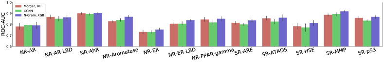
(a) ROC-AUC of the best models on Tox21 (Morgan+RF, GCNN, N-gram+XGB). Larger is better.

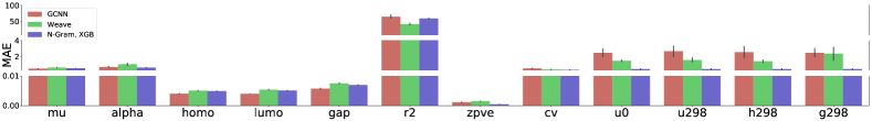
(b) MAE of the best models on QM9 (GCNN, Weave, N-gram+XGB). Smaller is better.

Figure 2: Performance of the best models on the datasets Tox21 and QM9, averaged over 5-fold cross-validation.

Performance.

Table 2 summarizes the prediction performance of the methods on all 60 tasks. Since (1) no method can consistently beat all other methods on all tasks, and (2) for datasets like QM8, the error (MAE) of the best models are all close to 0, we report both the top-1 and top-3 number of tasks each method obtained. Such high-level overview can help better understand the model performance. Complete results are included in Appendix H.

Overall, we observe that N-gram graph, especially using XGBoost, shows better performance than the other methods. N-gram with XGBoost is in top-1 for 21 out of 60 tasks, and is in top-3 for 48. On some tasks, the margin is not large but the advantage is consistent; see for example the tasks on the dataset Tox21 in Figure 2(a). On some tasks, the advantage is significant; see for example the tasks u0, u298, h298, g298 on the dataset QM9 in Figure 2(b).

We also observe that random forest on Morgan fingerprints has performance beyond general expectation, in particular, better than the recent graph neural network models on the classification tasks. One possible explanation is that we have used up to 4000 trees and obtained improved performance compared to 75 trees as in [56], since the number of trees is the most important parameter as pointed out in [37]. It also suggests that Morgan fingerprints indeed contains sufficient amount of information for the classification tasks, and methods like random forest are good at exploiting them.

Transferable Vertex Embedding.

An intriguing property of the vertex embeddings is that they can be transferred across datasets. We evaluate N-Gram graph with XGB on Tox21, using different vertex embeddings: trained on Tox21, random, and trained on other datasets. See details in Section G.1. Table 3 shows that embeddings from other datasets can be used to get comparable results. Even random embeddings can get good results, which is explained in Section 4.

Table 3: AUC-ROC of N-Gram graph with XGB on 12 tasks from Tox21. Six vertex embeddings are considered: non-transfer (trained on Tox21), vertex embeddings generated randomly and learned from 4 other datasets.

	Non-Transfer	Random	Delaney	CEP	MUV	Clintox
NR-AR	0.791	0.790	0.785	0.787	0.796	0.780
NR-AR-LBD	0.864	0.846	0.863	0.849	0.864	0.867
NR-AhR	0.902	0.895	0.903	0.892	0.901	0.903
NR-Aromatase	0.869	0.858	0.867	0.848	0.858	0.866
NR-ER	0.753	0.751	0.752	0.740	0.735	0.747
NR-ER-LBD	0.838	0.820	0.843	0.820	0.827	0.847
NR-PPAR-gamma	0.851	0.809	0.862	0.813	0.832	0.857
SR-ARE	0.835	0.823	0.841	0.814	0.835	0.842
SR-ATAD5	0.860	0.830	0.844	0.817	0.845	0.857
SR-HSE	0.812	0.777	0.806	0.768	0.805	0.810
SR-MMP	0.918	0.909	0.918	0.902	0.916	0.919
SR-p53	0.868	0.856	0.869	0.841	0.856	0.870

Computational Cost.

Table 4 depicts the representation construction time of different methods. Since vertex embeddings can be amortized across different tasks on the same dataset or even transferred, the main runtime of our method is from the graph embedding step. It is relatively efficient, much faster than the GNNs and the kernel method, though Morgan fingerprints can be even faster.

Table 4: Representation construction time in seconds. One task from each dataset as an example. Average over 5 folds, and including both the training set and test set.

Task	Dataset	WL CPU	Morgan FPs CPU	GCNN GPU	Weave GPU	GIN GPU	Vertex, Emb GPU	Graph, Emb GPU
Delaney	Delaney	2.46	0.25	39.70	65.82	–	49.63	2.90
Malaria	Malaria	128.81	5.28	377.24	536.99	–	1152.80	19.58
CEP	CEP	1113.35	17.69	607.23	849.37	–	2695.57	37.40
QM7	QM7	60.24	0.98	103.12	76.48	–	173.50	10.60
E1-CC2	QM8	584.98	3.60	382.72	262.16	–	966.49	33.43
mu	QM9	–	19.58	9051.37	1504.77	–	8279.03	169.72
NR-AR	Tox21	70.35	2.03	130.15	142.59	608.57	525.24	10.81
CT-TOX	Clintox	4.92	0.63	62.61	95.50	135.68	191.93	3.83
MUV-466	MUV	276.42	6.31	401.02	690.15	1327.26	1221.25	25.50
HIV	HIV	2284.74	17.16	1142.77	2138.10	3641.52	3975.76	139.85

Comparison to models using 3D information.

What makes molecular graphs more complicated is that they contain 3D information, which is helpful for making predictions [26]. Deep Tensor Neural Networks (DTNN) [47] and Message-Passing Neural Networks (MPNN) [26] are two graph neural networks that are able to utilize 3D information encoded in the datasets. Therefore, we further compare our method to these two most advanced GNN models, on the two datasets QM8 and QM9 that have 3D information. The results are summarized in Table 5. The detailed results are in Table S17 and the computational times are in Table S18. They show that our method, though not using 3D information, still gets comparable performance.

Table 5: Comparison of model using 3D information. On two regression datasets QM8 and QM9, and evaluated by MAE. N-Gram does not include any spatial information, like the distance between each atom pair, yet its performance is very comparative to the state-of-the-art methods.

Dataset	# Task	WL SVM	Morgan RF	Morgan XGB	GCNN	Weave	DTNN	MPNN	N-Gram RF	N-Gram XGB
QM8	12		1, 4	0, 1	4, 10	0, 3	0, 5	5, 6	0, 2	2, 5
QM9	12	–			0, 4	0, 1	7, 10	1, 9	0, 5	4, 7
Overall	24		1, 4	0, 1	4, 14	0, 4	7, 15	6, 15	0, 7	6, 12

Effect of $r$ and $T$.

We also explore the effect of the two key hyperparameters in N-Gram graph: the vertex embedding dimension $r$ and the N-gram length $T$. Figure 3 shows the results of 12 classification tasks on the Tox21 dataset are shown in, and Figure S2 shows the results on 3 regression tasks on the datasets Delaney, Malaria, and CEP. They reveal that generally, $r$ does not affect the model performance while increasing $T$ can bring in significant improvement. More detailed discussions are in appendix K.

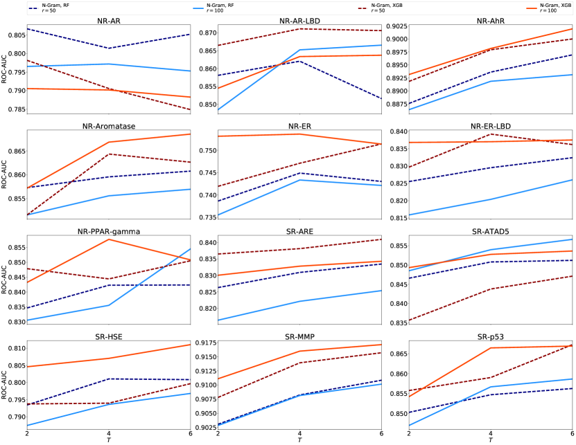
Figure 3: Effects of vertex embedding dimension $r$ and N-gram dimension $T$ on 12 tasks from Tox21: the effect of $r$ and $T$ on ROC-AUC. $x$-axis: the hyperparameter $T$; $y$-axis: ROC-AUC. Different lines correspond to different methods and different values of $r$.

6 Conclusion

This paper introduced a novel representation method called N-gram graph for molecule representation. It is simple, efficient, yet gives compact representations that can be applied with different learning methods. Experiments show that it can achieve overall better performance than prototypical traditional methods and several recent graph neural networks.

The method was inspired by the recent word embedding methods and the traditional N-gram approach in natural language processing, and can be formulated as a simple graph neural network. It can also be used to handle general graph-structured data, such as social networks. Concrete future works include applications on other types of graph-structured data, pre-training and fine-tuning vertex embeddings, and designing even more powerful variants of the N-gram graph neural network.

Appendix A Related Work

There are a large number of works along the line of machine learning for molecules and we review the more related ones here.

The adoption of sophisticated machine learning methods, in particular deep learning methods, has been recent trend in the domains of medicine, biology, chemistry, etc [14, 11, 16, 9]. Deep learning methods started to capture the attention among scientists in the drug discovery domain from Merck Molecular Activity Challange [40, 17]. Efforts expanded to investigate the benefits of multi-task deep neural networks, frequently showing outstanding performance when comparing with shallow models [38, 52, 37]. All of these works used Morgan fingerprints as input representations.

Another option for molecule representation is the SMILES string [54]. SMILES can be treated as a sequence of atoms and bonds, and each molecule has a unique canonical SMILES string among a frequently vast set of noncanonical, but completely valid, SMILES strings. Therefore, attempts were made to make SMILES feed into more complicated neural networks. [31] applied recurrent neural network language model (RNN) and convolutional neural networks (CNN) on SMILES, and showed that CNN is best when evaluated on the log-loss. SMILES as the representation is now common in molecule generation tasks. [27] first applied SMILES for automatic molecule design, and [34] proposed using a parser tree on SMILES so as to produce more grammatically-valid molecules, where the input is the one-hot encoded rules. On the other hand, [37] showed the limitation of SMILES and itself as a structured data is hard to interpret, and thus SMILES are not used in our experiments.

Molecular descriptors [50] is another representation, but it requires heuristically coming up with descriptors and dynamically adjusting it to tasks, which is not easy and requires a lot of domain knowledge. Therefore molecular descriptors are not considered in this paper since one of the goal here is to get a generalized feature representation.

Recent works started to explore the graph representation, and the benefit is its capability to encode the structured data. [19] first utilized message passing on graphs. At each step, this method passes the hidden message layer to the intermediate feature layer. The summed-up neural fingerprints are then fed into neural networks as features. Following this line of research, [2] made small adaptations by using the last message layer as feature inputs for neural network, and [60] proposed a differential pooling layer to learn the hierarchical information.

Other variants introduced different modules. [33] proposed a new module called weave for delivering information among atoms and bonds, and [39] used a weave operation with forward and backward operations across a molecule graph. [36] utilized edge information, and [20] generalized it into a message passing network framework, highlighting the importance of spatial information.

Viewing the molecules as graphs, the kernel method can be applied by using existing graph kernels (e.g., [48, 49]). The implicit feature mapping induced by the kernel can be viewed as the representation for the input. The Weisfeiler-Lehman kernel [49] is particularly related due to its efficiency and theoretical backup. It is also similar in spirit to the Morgan fingerprints and closely related to the recent GIN graph neural network [58].

Appendix B Background and Preliminaries

Generally, molecules can be viewed as graphs on atoms together with attribute information of the atoms, and we assume our molecule datasets are given in the format. To apply learning methods, they are converted to feature vectors (fingerprints), or are directly handled by specifically designed learning models (graph neural networks). The fingerprints or the hidden layers of graph neural networks are regarded as the representations or embeddings of the graphs.

B.1 Raw Data: Representation as Graphs With Vertex Attributes

Nearly all molecules can be potentially represented as a graph, where each atom is a vertex and each bond is an edge. Suppose there are $m$ vertices in the graph, denoted as $i\in\{0,1,...,m-1\}$. Each vertex entails useful attribute information, like the atom symbol and number of charges for atom vertices. These vertex attributes are encoded into a vertex attribute matrix $\mathcal{V}\in\{0,1\}^{m\times S}$, where $S$ is the number of attributes. A concrete example is given by the following:

$$\mathcal{V}_{i,\cdot}=[\mathcal{V}_{i,0},\mathcal{V}_{i,1},\ldots,\mathcal{V}_{i,6},\mathcal{V}_{i,7}],$$

$$\text{atom symbol }\mathcal{V}_{i,0}\in\{\text{C},\text{Cl},\text{I},\text{F},\ldots\},$$

$$\text{atom degree }\mathcal{V}_{i,1}\in\{0,1,2,3,4,5,6\},$$

$$\ldots$$

$$\text{is acceptor }\mathcal{V}_{i,6}\in\{0,1\},$$

$$\text{is donor }\mathcal{V}_{i,7}\in\{0,1\}.$$ (6)

Note that the attributes typically have discrete values.

The bonding information is encoded into the adjacency matrix $\mathcal{A}\in\{0,1\}^{m\times m}$, where $\mathcal{A}_{i,j}=1$ if and only if two vertices $i$ and $j$ are linked.

We let $G=(\mathcal{V},\mathcal{A})$ denote a molecular graph.

B.2 Fingerprints

We review two prototype methods here. Morgan fingerprints and its variants [42] have been one of the most widely used featurization methods in virtual screening. It is an iterative algorithm that encodes the circular substructures of the molecule as identifiers at increasing levels with each iteration. In each iteration, hashing is applied to generate new identifiers, and thus, there is a chance that two substructures are represented by the same identifier. In the end, a list of identifiers encoding the substructures is folded to bit positions of a fixed-length bit string. A 1-bit at a particular position indicates the presence of a substructure (or multiple substructures if they are all hashed to this position) and a 0-bit indicates the absence of corresponding substructures. Due to the hashing collisions, it is difficult to interpret such fingerprints and examine how the machine learning systems utilize them.

Figure S1: Illustration of the Morgan fingerprint and SMILES molecule representations. The molecule is displayed on a 2D space. The corresponding canonical SMILES is c1cc(oc1C(=O)Nc2nc(cs2)C(=O)OCC)Br, and Morgan Fingerprints is, for example, [000000…00100100100…000000].

Another prototypical method, Simplified Molecular Input Line Entry System (SMILES) [54], is a character sequence describing molecular structures. There are some inherent issues in SMILES, the biggest being that molecules cannot be simply represented as a linear sequence: the properties of drug-like organic molecules usually have dependence on ring structures and tree-like branching, whose information is lost in a linear sequence. Our experiments show that it generally achieves worse performance than the other methods, so it is not considered as a competitor in the experimental section.

One example of molecule as a graph is shown in Figure S1, together with its Morgan fingerprint and SMILES molecule representations.

B.3 Graph Neural Networks

In recent works, message passing has been dominant in graph neural networks [25, 30, 61, 57]. A GNN keeps a vector $h_{i}$ for each vertex $i$ and uses some neighborhood aggregation strategy that iteratively updates the vector by aggregating those of its neighbors. After $t$ iterations, each vertex is able to capture the information of the vertices at most $t$-hops away. Formally, the $k$-th iteration is to compute

$$f_{i}^{(k)} =\text{AGGREGATE}^{(k)}(\{h_{j}^{(k-1)}:j\in\text{Neighbor}(i)\}),$$

$$h^{(k)}_{i} =\text{COMBINE}^{(k)}(h_{i}^{(k-1)},f_{i}^{(k)}),$$ (7)

where $h^{(k)}_{i}$ is the value of $h_{i}$ at the $k$-th iteration, $h_{i}^{(0)}$ is typically initialized to the attribute vector of the vertex, and $\text{AGGREGATE}^{(k)}$ and $\text{COMBINE}^{(k)}$ are carefully chosen functions. The representation for the whole graph is then some aggregation of the vertex vectors. Such a framework has been used in the domains of molecules, but in general needs to be carefully specialized to this setting, see, e.g., [19, 2, 33].

Appendix C Complete Proofs for Theoretical Analysis

C.1 Preliminary

Here we provide a brief review of related concepts in the field of compressed sensing that are important for our analysis, following [3, 32]. For a review with details, please refer to [22].

The primary goal of compressed sensing is to recover a high-dimensional $k$-sparse signal $x\in\mathbb{R}^{N}$ from a few linear measurements. Here, being $k$-sparse means that $x$ has at most $k$ non-zero entries, i.e., $|x|_{0}\leq k$. In the noiseless case, we have a design matrix $A\in\mathbb{R}^{d\times N}$ and the measurement vector is $z=Ax$. The optimization formulation is then

$$\text{minimize}_{x^{\prime}}\|x^{\prime}\|_{0}\quad\text{subject to}\quad Ax^{\prime}=z$$ (8)

where $\|x^{\prime}\|_{0}$ is $\ell_{0}$ norm of $x^{\prime}$, i.e., the number of non-zero entries in $x^{\prime}$. The assumption that $x$ is the sparsest vector satisfying $Ax=z$ is equivalent to that $x$ is the optimal solution for (8).

Unfortunately, the $\ell_{0}$-minimization in (8) is NP-hard. The typical approach in compressed sensing is to consider its convex surrogate using $\ell_{1}$-minimization:

$$\text{minimize}_{x^{\prime}}\|x^{\prime}\|_{1}\quad\text{subject to}\quad Ax^{\prime}=z$$ (9)

where $\|x^{\prime}\|_{1}=\sum_{i}|x^{\prime}_{i}|$ is the $\ell_{1}$ norm of $x^{\prime}$. The fundamental question is when the optimal solution of (8) is equivalent to that of (9), i.e., when exact recovery is guaranteed.

C.1.1 The Restricted Isometry Property

One common condition for recovery is the Restricted Isometry Property (RIP):

Definition 2

$A\in\mathbb{R}^{d\times N}$ is $(\mathcal{X},\epsilon)$-RIP for some subset $\mathcal{X}\subseteq\mathbb{R}^{N}$ if for any $x\in\mathcal{X}$,

$$(1-\epsilon)\|x\|_{2}\leq\|Ax\|_{2}\leq(1+\epsilon)\|x\|_{2}.$$

We will abuse notation and say $(k,\epsilon)$-RIP if $\mathcal{X}$ is the set of all $k$-sparse $x\in\mathbb{R}^{N}$.

Introduced by [13], RIP has been used to show to guarantee exact recovery.

Theorem 4 (Restatement of Theorem 1.1 in [12])

Suppose $A$ is $(2k,\epsilon)$-RIP for an $\epsilon<\sqrt{2}-1$. Let $\hat{x}$ denote the solution to (9), and let $x_{k}$ denote the vector $x$ with all but the k-largest entries set to zero. Then

$$\|\hat{x}-x\|_{1}\leq C_{0}\|x_{k}-x\|_{1}$$

and

$$\|\hat{x}-x\|_{2}\leq C_{0}k^{-1/2}\|x_{k}-x\|_{1}.$$

In particular, if $x$ is $k$-sparse, the recovery is exact.

Furthermore, it has been shown that $A$ is $(k,\epsilon)$-RIP with overwhelming probability when $d=\Omega(k\log\frac{N}{k})$ and $\sqrt{d}A_{ij}\sim\mathcal{N}(0,1)(\forall i,j)$ or $\sqrt{d}A_{ij}\sim\mathcal{U}\{-1,1\}(\forall i,j)$.

For our purpose, we also concern about whether the $\ell$-way column Hadamard-product of $A$ has RIP.

Definition 3 ($\ell$-way Column Hadamard Product)

Let $A$ be a $d\times N$ matrix, and let $\ell$ be a natural integer. The $\ell$-way column Hadamard-product of $A$ is a $d\times{N\choose\ell}$ matrix denoted as $A^{(\ell)}$, whose columns indexed by a sequence $1\leq i_{1}<i_{2}\cdots<i_{\ell}\leq d$ is the element-wise product of the $i_{1},i_{2},\dots,i_{\ell}$-th columns of $A$, i.e., $(i_{1},i_{2},\dots,i_{\ell})$-th column in $A^{(\ell)}$ is $A_{i_{1}}\odot A_{i_{2}}\odot\cdots\odot A_{i_{\ell}}$ where $A_{j}$ for $j\in[N]$ is the $j$-th column in $A$.

We have the following theorems:

Theorem 5 (Restatement of Theorem 4.1 in [32])

Let $X$ be an $n\times d$ matrix, and let $A$ be a $d\times N$ random matrix with independent entries $R_{ij}$ such that $\mathbb{E}[R_{ij}]=0,\mathbb{E}[R_{ij}]=1$, and $|R_{ij}|\leq\tau$ almost surely. Let $\epsilon\in(0,1)$, and let $k$ be an integer satisfying $\text{sr}(X)\geq\frac{C\tau^{8}}{\epsilon^{2}}k^{2}\log\frac{N^{2}}{k\epsilon}$ for some universal constant $C>0$. Then with probability at least $1-\exp(-c\epsilon^{2}\text{sr}(X)/(k^{2}\tau^{8}))$ for some universal constant $c>0$, the matrix $XA^{(\ell)}/\|X\|_{F}$ is $(k,\epsilon)$-RIP.

Here, $\text{sr}(X)=\|X\|_{F}^{2}/\|X\|^{2}$ is the stable rank of $X$. In our case, we will apply the theorem with $X$ being $\mathbf{I}_{d\times d}/\sqrt{d}$ where $\mathbf{I}_{d\times d}\in\mathbb{R}^{d\times d}$ is the identity matrix.

Theorem 6 (Restatement of Theorem 4.3 in [32])

Let $X$ be an $n\times d$ matrix, and let $A$ be a $d\times N$ random matrix with independent entries $R_{ij}$ such that $\mathbb{E}[R_{ij}]=0,\mathbb{E}[R_{ij}]=1$, and $|R_{ij}|\leq\tau$ almost surely. Let $\ell\geq 3$ be a constant. Let $\epsilon\in(0,1)$, and let $k$ be an integer satisfying $\text{sr}(X)\geq\frac{C\tau^{4\ell}}{\epsilon^{2}}k^{3}\log\frac{N^{\ell}}{k\epsilon}$ for some universal constant $C>0$. Then with probability at least $1-\exp(-c\epsilon^{2}\text{sr}(X)/(k^{2}\tau^{4\ell}))$ for some universal constant $c>0$, the matrix $XA^{(\ell)}/\|X\|_{F}$ is $(k,\epsilon)$-RIP.

C.1.2 Compressed Learning

Given that $Ax$ preserves the information of sparse $x$ when $A$ is RIP, it is then natural to study the performance of a linear classifier learned on $Ax$ compared to that of the best linear classifier on $x$. Our analysis will use a theorem from [3] that generalizes that of [10].

Let $\mathcal{X}\subseteq\mathbb{R}^{N}$ denote

$$\mathcal{X}=\{x:x\in\mathbb{R}^{N},\|x\|_{0}\leq k,\|x\|_{2}\leq B\}.$$

Let $\{(x_{i},y_{i})\}_{i=1}^{M}$ be a set of $M$ samples i.i.d. from some distribution over $\mathcal{X}\times\{-1,1\}$. Let $\ell$ denote a $\lambda_{\ell}$-Lipschitz convex loss function. Let $\ell_{\mathcal{D}}(\theta)$ denote the risk of a linear classifier with weight $\theta\in\mathbb{R}^{N}$, i.e., $\ell_{\mathcal{D}}(\theta)=\mathbb{E}[\ell(\langle\theta,x\rangle,y)]$, and let $\theta^{*}$ denote a minimizer of $\ell_{\mathcal{D}}(\theta)$. Let $\ell^{A}_{\mathcal{D}}(\theta)$ denote the risk of a linear classifier with weight $\theta\in\mathbb{R}^{d}$ over $Ax$, i.e., $\ell^{A}_{\mathcal{D}}(\theta_{A})=\mathbb{E}[\ell(\langle\theta_{A},Ax\rangle,y)]$, and let $\hat{\theta}_{A}$ denote the weight learned with $\ell_{2}$-regularization over $\{(Ax_{i},y_{i})\}_{i}$:

$$\hat{\theta}_{A}=\arg\min_{\theta}\frac{1}{M}\sum_{i=1}^{M}\ell(\langle\theta,Ax_{i}\rangle,y_{i})+\lambda\|\theta\|_{2}$$ (10)

where $\lambda$ is the regularization coefficient.

Theorem 7 (Restatement of Theorem 4.2 in [3])

Suppose $A$ is $(\Delta\mathcal{X},\epsilon)$-RIP. Then with probability at least $1-\delta$,

$$\ell^{A}_{\mathcal{D}}(\hat{\theta}_{A})\leq\ell_{\mathcal{D}}(\theta^{*})+O\left(\lambda_{\ell}B\|\theta^{*}\|\sqrt{\epsilon+\frac{1}{M}\log\frac{1}{\delta}}\right)$$

for appropriate choice of $C$. Here, $\Delta\mathcal{X}=\{x-x^{\prime}:x,x^{\prime}\in\mathcal{X}\}$ for any $\mathcal{X}\subseteq\mathbb{R}^{N}$.

C.2 Representation Power

In this subsection, we provide the proof of Theorem 1.

We begin by defining the distribution over the vertex embedding matrix $W$. Recall that $k_{j}$ is the number of possible values for the $j$-th attribute. Suppose we have numbers $r_{j}\in(0,r)$ so that $\sum_{j=0}^{S-1}r_{j}=r$ whose values will be specified later. Let

$$W=\begin{bmatrix}U^{0}&0&\cdots&0\\ 0&U^{1}&\cdots&0\\ \cdots&\cdots&\cdots&\cdots\\ 0&0&\cdots&U^{S-1}\end{bmatrix}$$ (11)

where $U^{j}\in\mathbb{R}^{r_{j}\times k_{j}}$. Now let’s specify $U^{j}$. Let the entries in $U^{j}$’s are independent random variables, and let the entries be uniform from $\{-1,1\}$ with some scaling factor $c_{u}$, i.e., $(U^{j})_{ik}\sim c_{u}\times\mathcal{U}\{-1,1\}$, where the value of $c_{u}$ will be determined later.

Now, let $(U^{j})^{(n)}$ denote the $n$-way column Hadamard product of $U^{j}$, and let

$$T_{(n)}=\begin{bmatrix}(U^{0})^{(n)}&0&\cdots&0\\ 0&(U^{1})^{(n)}&\cdots&0\\ \cdots&\cdots&\cdots&\cdots\\ 0&0&\cdots&(U^{S-1})^{(n)}\end{bmatrix}$$ (12)

Then it can be verified that

$$f_{(n)}=T_{(n)}c_{(n)}.$$ (13)

Now we can apply Theorem 5 for $n=2$ and Theorem 6 for $n\geq 3$ on each $(U^{j})^{(n)}$. Let $s_{n,j}$ denote the sparsity of $c^{(j)}_{(n)}$. Then with $r_{j}\geq\Omega(ns_{n,j}^{3}\log k_{j})$ and appropriate set scaling factor $c_{u}$, we have that with probability at least $1-\exp(-cr_{j}/s_{n,j}^{2})$, $(U^{j})^{(n)}$ is $(2s_{n,j},\epsilon)$-RIP for $\epsilon=0.1$. This then means that $f_{n}$ can be exactly recovered from $c_{(n)}$ by Theorem 4. Now, by setting $r=\Omega(ns_{n}^{3}\log K)$ where $s_{n}=\sum_{j=0}^{S-1}s_{n,j}$, we can choose $r_{j}$’s satisfying $r_{j}=\Omega(ns_{n,j}^{3}\log k_{j}+r/S)$. Furthermore, we have $r_{j}/s_{n,j}^{2}=\Omega(r_{j}^{1/3})=\Omega((r/S)^{1/3})$, so the failure probability is bounded by $S\exp(-c(r/S)^{1/3})$.

C.3 Prediction Power

Proof of Theorem 2.

Theorem 2 is a direct consequence of Theorem 1.

By Theorem 1, under the conditions, we have that there exists a mapping $\mathcal{M}_{(n)}$ from $f_{G}$ to $c_{(n)}$. Therefore, there exists a mapping $\mathcal{M}_{[T]}$ from $f_{G}$ to $c_{[T]}$, by applying $\mathcal{M}_{(n)}$’s on each blocks of $f_{G}$, respectively. Now, define $g_{f}=g_{c}\circ\mathcal{M}_{[T]}$, such that $g_{f}(f_{G})=g_{c}\circ\mathcal{M}_{[T]}(f_{G})=g_{c}(c_{[T]})$, so $\ell_{\mathcal{D}}(g_{f})=\ell_{\mathcal{D}}(g_{c})$.

Proof of Theorem 3

Let

$$T_{[T]}=\begin{bmatrix}T_{(1)}&0&\cdots&0\\ 0&T_{(2)}&\cdots&0\\ \cdots&\cdots&\cdots&\cdots\\ 0&0&\cdots&T_{(T)}\end{bmatrix}$$ (14)

where $T_{(n)}(1\leq n\leq T)$ is defined as in (12). Then it can be verified that

$$f_{G}=T_{[T]}c_{[T]}.$$ (15)

Under the specified conditions we have that with high probability $T_{(n)}$’s are $(2s_{n},\epsilon)$-RIP, so $T_{[T]}$ is $(\Delta\mathcal{X},\epsilon)$-RIP. Since the logistic loss is 1-Lipschitz convex, the statement follows from Theorem 7, while the failure probability follows from a union bound.

Appendix D Task Specification

Table S1: Number of positives and all molecules on 12 Tox21 tasks.

Task	Num of Positives	Total Number	Positive Ratio (%)
NR-AR	304	7332	4.14621
NR-AR-LBD	237	6817	3.47660
NR-AhR	783	6592	11.87803
NR-Aromatase	298	5853	5.09141
NR-ER	784	6237	12.57015
NR-ER-LBD	347	7014	4.94725
NR-PPAR-gamma	186	6505	2.85934
SR-ARE	954	5907	16.15033
SR-ATAD5	262	7140	3.66947
SR-HSE	378	6562	5.76044
SR-MMP	912	5834	15.63250
SR-p53	414	6814	6.07573

Table S2: Number of positives and all molecules on 2 ClinTox tasks

Task	Num of Positives	Total Number	Positive Ratio (%)
CT_TOX	112	1469	7.62423
FDA_APPROVED	1375	1469	93.60109

Table S3: Number of positives and all molecules on 17 MUV tasks.

Task	Num of Positives	Total Number	Positive Ratio (%)
MUV-466	27	14844	0.18189
MUV-548	29	14737	0.19678
MUV-600	30	14734	0.20361
MUV-644	30	14633	0.20502
MUV-652	29	14903	0.19459
MUV-689	29	14606	0.19855
MUV-692	30	14647	0.20482
MUV-712	28	14415	0.19424
MUV-713	29	14841	0.19540
MUV-733	28	14691	0.19059
MUV-737	29	14696	0.19733
MUV-810	29	14646	0.19801
MUV-832	30	14676	0.20442
MUV-846	30	14714	0.20389
MUV-852	29	14658	0.19784
MUV-858	29	14775	0.19628
MUV-859	24	14751	0.16270

Table S4: Number of positives and all molecules on 1 HIV task.

Task	Num of Positives	Total Number	Positive Ratio (%)
HIV	1425	41023	3.47366

Appendix E Atom Feature Specification

Tables S5 and S6 show the types of feature attributes for the atoms in the molecules of the datasets used in our experiments. Also in Appendix L, we can observe that the selection of feature attribute values, especially adding more atom symbols, has very limited improvement.

Table S5: $d=42$ features are divided into $S=8$ attributes. Each feature attribute corresponds to one type of atom property, including atom symbol, atom degree, atom charge, etc. Note that it is hard to enumerate all the values for the atom properties, so we use the last bit ’Unknown’ as the placeholder to catch the missing symbols.

id	digit	property	values
0	0-9	atom symbol	[C, Cl, I, F, O, N, P, S, Br, Unknown]
1	10-16	atom degree	[0, 1, 2, 3, 4, 5, Unknown]
2	17-23	number of Hydrogen	[0, 1, 2, 3, 4, 5, Unknown]
3	24-29	implicit valence	[0, 1, 2, 3, 4, Unknown]
4	30-35	atom charge	[-2, -1, 0, 1, 2, Unknown]
5	36-37	is aromatic	[no, yes]
6	38-39	is acceptor	[no, yes]
7	40-41	is donor	[no, yes]

Table S6: On datasets QM8 and QM9, due to the input format of the molecule file, we cannot extract the atom attributes like the number of hydrogen, is-acceptor and is-donor property (while keeping its 3D information at the same time). So following [56], only $d=32$ features, i.e., $S=5$ attributes are considered.

id	digit	property	values
0	0-9	atom symbol	[C, Cl, I, F, O, N, P, S, Br, Unknown]
1	10-16	atom degree	[0, 1, 2, 3, 4, 5, Unknown]
2	17-23	implicit valence	[0, 1, 2, 3, 4, 5, Unknown]
3	24-29	atom charge	[-2, -1, 0, 1, 2, Unknown]
4	30-31	is aromatic	[no, yes]

Appendix F Hyperparameter Tuning

F.1 Hyperparameters for Representation

Morgan Fingerprints.

To generate Morgan fingerprints, we use the public package RdKit [35] and follow the hyperparameters from benchmark [44]: the number of bits is 1024 and radius is 2.

Graph Neural Networks.

For Graph CNN, Weave Neural Network, Deep Tensor Neural Network, and Message-Passing Neural Network, we follow the optimal hyperparameter schemes provided in [56]. Note that they are tuned for each of these datasets, respectively, to guarantee the optimality.

N-Gram Graph.

The hyperparameters for N-gram graph are included in Table S7, and the effects of two important hyperparameters (random dimension $r$ and n-gram number $T$) will be discussed in Appendix K.

Table S7: Hyperparameter sweeping for N-Gram Graph. We have $S=8$ feature attributes.

Hyperparameters	Candidate values
Random Dimension $r$	50, 100
N-Gram Num $T$	2, 4, 6
Embedding Structure	[Embedding -> Sum], [Embedding -> Mean]
Neural Network	[$r$, 20, $S$], [$r$, 100, $S$] , [$r$, 100, 20, $S$]

F.2 Hyperparameters for Modeling

For other baseline models, we run a grid search for hyperparameter sweeping, including Weisfeiler-Lehman Graph Kernel in Table S8, random forest in Table S9, XGBoost in Table S10, and Graph Isomorphism Network Table S11.

Table S8: Hyperparameter sweeping for Weisfeiler-Lehman Graph Kernel.

Hyperparameters	Candidate values
Number of Step	1, 2, 3

Table S9: Hyperparameter sweeping for Random Forest.

Hyperparameters	Candidate values
Number of Trees	100, 4000
Max Features	None, sqrt, log2
Min Samples Leaf	1, 10, 100, 1000
Class Weight	None, balanced_subsample, balanced

Table S10: Hyperparameter sweeping for XGBoost.

Hyperparameters	Candidate values
Max Depth	5, 10, 50, 100
Learning Rate	1, 3e-1, 1e-1, 3e-2
Number of Trees	30, 100, 300, 1000, 3000

Table S11: Hyperparameter sweeping for Graph Isomorphism Network.

Hyperparameters	Candidate values
Max Depth	2, 3, 5
Hidden Dimension	30, 50
Epoch	100, 300
Optimizer	SGD, Adam
Learning Rate Scheduler	None, ReduceLROnPlateau, StepLR

Appendix G Vertex Embedding

The CBoW-like neural network structure is displayed in Figure 1. Though the vertex embedding step is unsupervised, we still follow the 5-fold cross-validation, so as not to touch the test set before prediction. In other words, we will create 5 CBoW-like models for each task (or dataset ) and each vertex embedding dimension $R$. We report the test accuracy during vertex embedding in Table S12.

Table S12: The mean accuracy of 5-fold cross-validation in vertex embedding. The accuracy measures how the CBoW-like neural network can accurately predict the vertex attributes.

Task/Dataset	Accuracy(%), $r=50$	Accuracy(%), $r=100$
Delaney	$0.924\pm 0.001$	$0.924\pm 0.001$
Malaria	$0.937\pm 0.001$	$0.938\pm 0.000$
CEP	$0.923\pm 0.001$	$0.923\pm 0.000$
QM7	$0.898\pm 0.001$	$0.897\pm 0.001$
QM8	$0.988\pm 0.000$	$0.988\pm 0.000$
QM9	$0.987\pm 0.000$	$0.987\pm 0.001$
NR-AR	$0.916\pm 0.000$	$0.916\pm 0.000$
NR-AR-LBD	$0.915\pm 0.001$	$0.914\pm 0.003$
NR-AhR	$0.916\pm 0.000$	$0.915\pm 0.000$
NR-Aromatase	$0.915\pm 0.000$	$0.915\pm 0.000$
NR-ER	$0.915\pm 0.001$	$0.914\pm 0.001$
NR-ER-LBD	$0.916\pm 0.001$	$0.915\pm 0.001$
NR-PPAR-gamma	$0.914\pm 0.000$	$0.915\pm 0.000$
SR-ARE	$0.915\pm 0.000$	$0.915\pm 0.000$
SR-ATAD5	$0.916\pm 0.000$	$0.916\pm 0.000$
SR-HSE	$0.915\pm 0.000$	$0.915\pm 0.000$
SR-MMP	$0.913\pm 0.001$	$0.914\pm 0.001$
SR-p53	$0.915\pm 0.000$	$0.915\pm 0.001$
Clintox	$0.911\pm 0.001$	$0.911\pm 0.000$
MUV-466	$0.940\pm 0.001$	$0.940\pm 0.000$
MUV-548	$0.932\pm 0.001$	$0.931\pm 0.001$
MUV-600	$0.938\pm 0.000$	$0.937\pm 0.001$
MUV-644	$0.932\pm 0.001$	$0.932\pm 0.000$
MUV-652	$0.939\pm 0.000$	$0.939\pm 0.001$
MUV-689	$0.942\pm 0.001$	$0.942\pm 0.001$
MUV-692	$0.934\pm 0.001$	$0.934\pm 0.000$
MUV-712	$0.938\pm 0.001$	$0.938\pm 0.001$
MUV-713	$0.938\pm 0.000$	$0.937\pm 0.000$
MUV-733	$0.937\pm 0.001$	$0.937\pm 0.001$
MUV-737	$0.940\pm 0.001$	$0.939\pm 0.001$
MUV-810	$0.937\pm 0.000$	$0.937\pm 0.000$
MUV-832	$0.937\pm 0.001$	$0.936\pm 0.001$
MUV-846	$0.938\pm 0.000$	$0.938\pm 0.000$
MUV-852	$0.937\pm 0.001$	$0.937\pm 0.001$
MUV-858	$0.938\pm 0.001$	$0.938\pm 0.001$
MUV-859	$0.939\pm 0.001$	$0.939\pm 0.001$
HIV	$0.920\pm 0.001$	$0.919\pm 0.001$

G.1 Transferable Vertex Embedding

The complete process for getting Table 3 is as follows.

Vertex Embedding. Train the unsupervised CBoW model for vertex embedding $W$ on all the molecules from the source dataset. For random projection, we just initialize parameters of the CBoW model under the Gaussian distribution, and only molecules for that task is used if it comes from Tox21, i.e., the non-transfer case.

Graph Embedding. Apply $W$ on molecules from target task for the graph embedding, $f_{G}$. Then train the model based on $f_{G}$.

Appendix H Complete Results on 60 Regression and Classification Tasks

Table S13: Here we include the performance on 28 regression tasks with 7 models. All experiments are done on a 5-fold cross-validation, and the mean evaluation of 5 runs is reported here. The top-3 models are bolded, and the best model is underlined.

Task	Eval Metric	WL SVM	Morgan RF	Morgan XGB	GCNN	Weave	N-Gram RF	N-Gram XGB
Delaney	RMSE	1.265	1.168	3.063	0.825	0.687	0.769	0.731
Malaria	RMSE	1.094	0.983	1.943	1.144	1.487	1.022	1.019
CEP	RMSE	1.800	1.300	3.049	1.493	2.846	1.399	1.366
QM7	MAE	176.750	127.662	110.230	76.637	62.560	57.747	53.919
E1-CC2	MAE	0.032	0.008	0.008	0.006	0.007	0.008	0.007
E2-CC2	MAE	0.023	0.010	0.010	0.008	0.007	0.009	0.008
f1-CC2	MAE	0.072	0.014	0.015	0.014	0.018	0.015	0.015
f2-CC2	MAE	0.081	0.032	0.033	0.031	0.036	0.033	0.031
E1-PBE0	MAE	0.034	0.008	0.008	0.006	0.006	0.008	0.007
E2-PBE0	MAE	0.029	0.010	0.010	0.007	0.008	0.008	0.008
f1-PBE0	MAE	0.068	0.012	0.013	0.012	0.014	0.013	0.013
f2-PBE0	MAE	0.078	0.026	0.027	0.024	0.027	0.025	0.024
E1-CAM	MAE	0.033	0.007	0.007	0.006	0.006	0.007	0.007
E2-CAM	MAE	0.025	0.009	0.009	0.006	0.006	0.008	0.007
f1-CAM	MAE	0.073	0.013	0.014	0.013	0.016	0.014	0.014
f2-CAM	MAE	0.080	0.028	0.028	0.026	0.031	0.028	0.026
average		0.052	0.015	0.015	0.013	0.015	0.015	0.014
mu	MAE	–	0.548	0.533	0.482	0.624	0.562	0.535
alpha	MAE	–	3.787	2.672	0.685	1.034	0.722	0.612
homo	MAE	–	0.006	0.006	0.004	0.005	0.005	0.005
lumo	MAE	–	0.007	0.006	0.004	0.005	0.006	0.005
gap	MAE	–	0.008	0.008	0.006	0.008	0.007	0.007
r2	MAE	–	94.815	82.516	64.775	42.095	72.846	59.137
zpve	MAE	–	0.009	0.007	0.001	0.002	0.001	0.000
cv	MAE	–	1.505	1.166	0.524	0.374	0.434	0.334
u0	MAE	–	16.410	12.736	2.460	1.465	0.429	0.427
u298	MAE	–	16.410	12.757	2.671	1.560	0.429	0.428
h298	MAE	–	16.411	12.752	2.542	1.414	0.428	0.428
g298	MAE	–	16.414	12.750	2.466	2.359	0.428	0.428
average		–	13.823	11.476	6.474	4.187	6.357	5.152

Table S14: Here we include the performance on 32 classification tasks with 8 models. All experiments are done on a 5-fold cross-validation, and the mean evaluation of 5 runs is reported here. The top-3 models are bolded, and the best model is underlined.

Task	Eval Metric	WL SVM	Morgan RF	Morgan XGB	GCNN	Weave	GIN	N-Gram RF	N-Gram XGB
NR-AR	ROC-AUC	0.759	0.781	0.780	0.793	0.789	0.755	0.797	0.791
NR-AR-LBD	ROC-AUC	0.843	0.868	0.853	0.851	0.835	0.826	0.871	0.864
NR-AhR	ROC-AUC	0.879	0.900	0.894	0.894	0.870	0.880	0.894	0.902
NR-Aromatase	ROC-AUC	0.849	0.828	0.780	0.839	0.819	0.818	0.858	0.869
NR-ER	ROC-AUC	0.716	0.731	0.722	0.731	0.712	0.688	0.747	0.753
NR-ER-LBD	ROC-AUC	0.794	0.806	0.795	0.806	0.808	0.778	0.827	0.838
NR-PPAR-gamma	ROC-AUC	0.819	0.844	0.805	0.817	0.794	0.800	0.856	0.851
SR-ARE	ROC-AUC	0.803	0.814	0.800	0.799	0.771	0.788	0.826	0.835
SR-ATAD5	ROC-AUC	0.819	0.854	0.829	0.825	0.778	0.814	0.857	0.860
SR-HSE	ROC-AUC	0.798	0.782	0.770	0.772	0.751	0.723	0.798	0.812
SR-MMP	ROC-AUC	0.887	0.886	0.878	0.894	0.887	0.866	0.911	0.918
SR-p53	ROC-AUC	0.835	0.859	0.796	0.834	0.795	0.819	0.859	0.868
average		0.813	0.827	0.806	0.821	0.798	0.791	0.841	0.842
CT_TOX	ROC-AUC	0.837	0.788	0.840	0.872	0.859	0.823	0.857	0.873
FDA_APPROVED	ROC-AUC	0.851	0.784	0.830	0.875	0.836	0.848	0.825	0.874
average		0.833	0.787	0.847	0.868	0.834	0.837	0.837	0.870
MUV-466	PR-AUC	0.046	0.076	0.058	0.003	0.017	0.060	0.058	0.086
MUV-548	PR-AUC	0.178	0.230	0.259	0.065	0.065	0.070	0.073	0.094
MUV-600	PR-AUC	0.023	0.021	0.017	0.004	0.006	0.013	0.007	0.009
MUV-644	PR-AUC	0.149	0.185	0.225	0.034	0.025	0.124	0.046	0.064
MUV-652	PR-AUC	0.164	0.095	0.039	0.020	0.021	0.022	0.085	0.118
MUV-689	PR-AUC	0.030	0.025	0.094	0.011	0.013	0.021	0.026	0.046
MUV-692	PR-AUC	0.003	0.010	0.003	0.004	0.003	0.006	0.005	0.005
MUV-712	PR-AUC	0.208	0.119	0.158	0.062	0.075	0.192	0.134	0.151
MUV-713	PR-AUC	0.036	0.057	0.024	0.007	0.011	0.007	0.026	0.026
MUV-733	PR-AUC	0.076	0.080	0.046	0.011	0.005	0.016	0.021	0.047
MUV-737	PR-AUC	0.058	0.056	0.060	0.008	0.017	0.005	0.084	0.080
MUV-810	PR-AUC	0.139	0.186	0.215	0.010	0.006	0.033	0.013	0.022
MUV-832	PR-AUC	0.365	0.556	0.508	0.029	0.032	0.388	0.229	0.280
MUV-846	PR-AUC	0.369	0.299	0.407	0.219	0.250	0.397	0.250	0.220
MUV-852	PR-AUC	0.405	0.173	0.300	0.159	0.131	0.337	0.214	0.238
MUV-858	PR-AUC	0.079	0.090	0.018	0.006	0.003	0.051	0.014	0.015
MUV-859	PR-AUC	0.004	0.004	0.007	0.005	0.004	0.003	0.007	0.006
average		0.154	0.146	0.158	0.041	0.047	0.119	0.088	0.099
HIV	ROC-AUC	0.800	0.849	0.827	0.805	0.663	0.785	0.828	0.830

Appendix I N-Gram Walk vs. N-Gram Path

We compare N-Gram Path (the version of N-gram graph method that excludes walks containing two vertices with the same attribute values) and N-Gram Walk (the version of N-gram graph method that does not exclude such walks) on each of the 60 tasks. The same vertex embeddings are used, and both random forest (RF) and XGBoost (XGB) are experimented on top of the N-Gram graph embeddings. All regression tasks are shown in Table S15 and all classification tasks are shown in Table S16, and we can see that N-Gram Path is comparable to N-Gram Walk.

Table S15: Comparison of N-Gram Path-based graph and N-Gram Walk-based graph on 28 regression tasks. All experiments are done on a 5-fold cross-validation, and the mean evaluation of 5 runs is reported here. N-Gram Walk-based graph with XGB trained on top of it can excel on 27 out of the 28 regression tasks, while N-Gram Path achieves comparable performance.

Task	Eval Metric	N-Gram, RF Path	N-Gram, XGB Path	N-Gram, RF Walk	N-Gram, XGB Walk
Delaney	RMSE	0.866	0.746	0.769	0.731
Malaria	RMSE	1.036	1.027	1.022	1.019
CEP	RMSE	1.506	1.350	1.399	1.366
QM7	MAE	73.745	57.361	57.747	53.919
E1-CC2	MAE	0.011	0.009	0.008	0.007
E2-CC2	MAE	0.011	0.009	0.009	0.008
f1-CC2	MAE	0.017	0.016	0.015	0.015
f2-CC2	MAE	0.036	0.034	0.033	0.031
E1-PBE0	MAE	0.011	0.009	0.008	0.007
E2-PBE0	MAE	0.010	0.009	0.008	0.008
f1-PBE0	MAE	0.015	0.014	0.013	0.013
f2-PBE0	MAE	0.028	0.027	0.025	0.024
E1-CAM	MAE	0.010	0.008	0.007	0.007
E2-CAM	MAE	0.010	0.008	0.008	0.007
f1-CAM	MAE	0.017	0.015	0.014	0.014
f2-CAM	MAE	0.031	0.030	0.028	0.026
average		0.017	0.016	0.015	0.014
mu	MAE	0.629	0.588	0.562	0.535
alpha	MAE	0.868	0.759	0.722	0.612
homo	MAE	0.006	0.006	0.005	0.005
lumo	MAE	0.007	0.006	0.006	0.005
gap	MAE	0.009	0.008	0.007	0.007
r2	MAE	88.431	67.876	72.846	59.137
zpve	MAE	0.001	0.001	0.001	0.000
cv	MAE	0.613	0.498	0.434	0.334
u0	MAE	1.382	0.592	0.429	0.427
u298	MAE	1.384	0.594	0.429	0.428
h298	MAE	1.380	0.591	0.428	0.428
g298	MAE	1.382	0.593	0.428	0.428
average		8.035	6.001	6.357	5.152

Table S16: Comparison of N-Gram Path-based graph and N-Gram Walk-based graph on 32 classification tasks. All experiments are done on a 5-fold cross-validation, and the mean evaluation of 5 runs is reported here. N-Gram Walk-based graph with RF and XGB trained on top of it can excel on 5 and 15 tasks out of 32 respectively. Besides, the average performance trained with RF and XGB is better when using N-Gram walk-based graph, except for XGB on HIV. Overall, N-Gram Walk is better while N-Gram Path achieves comparable performance.

Task	Eval Metric	N-Gram, RF Path	N-Gram, XGB Path	N-Gram, RF Walk	N-Gram, XGB Walk
NR-AR	ROC-AUC	0.797	0.788	0.797	0.791
NR-AR-LBD	ROC-AUC	0.860	0.857	0.871	0.864
NR-AhR	ROC-AUC	0.890	0.896	0.894	0.902
NR-Aromatase	ROC-AUC	0.856	0.863	0.858	0.869
NR-ER	ROC-AUC	0.742	0.750	0.747	0.753
NR-ER-LBD	ROC-AUC	0.823	0.840	0.827	0.838
NR-PPAR-gamma	ROC-AUC	0.837	0.832	0.856	0.851
SR-ARE	ROC-AUC	0.824	0.834	0.826	0.835
SR-ATAD5	ROC-AUC	0.858	0.848	0.857	0.860
SR-HSE	ROC-AUC	0.790	0.795	0.798	0.812
SR-MMP	ROC-AUC	0.904	0.912	0.911	0.918
SR-p53	ROC-AUC	0.847	0.850	0.859	0.868
average		0.833	0.834	0.841	0.842
CT_TOX	ROC-AUC	0.838	0.858	0.857	0.873
FDA_APPROVED	ROC-AUC	0.816	0.854	0.825	0.874
average		0.810	0.855	0.837	0.870
MUV-466	PR-AUC	0.056	0.077	0.058	0.086
MUV-548	PR-AUC	0.088	0.100	0.073	0.094
MUV-600	PR-AUC	0.008	0.014	0.007	0.009
MUV-644	PR-AUC	0.061	0.093	0.046	0.064
MUV-652	PR-AUC	0.096	0.151	0.085	0.118
MUV-689	PR-AUC	0.027	0.025	0.026	0.046
MUV-692	PR-AUC	0.004	0.003	0.005	0.005
MUV-712	PR-AUC	0.088	0.085	0.134	0.151
MUV-713	PR-AUC	0.052	0.015	0.026	0.026
MUV-733	PR-AUC	0.017	0.015	0.021	0.047
MUV-737	PR-AUC	0.038	0.035	0.084	0.080
MUV-810	PR-AUC	0.017	0.054	0.013	0.022
MUV-832	PR-AUC	0.176	0.297	0.229	0.280
MUV-846	PR-AUC	0.245	0.223	0.250	0.220
MUV-852	PR-AUC	0.188	0.189	0.214	0.238
MUV-858	PR-AUC	0.007	0.016	0.014	0.015
MUV-859	PR-AUC	0.012	0.005	0.007	0.006
average		0.079	0.087	0.088	0.099
HIV	ROC-AUC	0.826	0.833	0.828	0.830

Appendix J Additional Experiments on Datasets with 3D Information

Since 3D information of the atoms in the molecules is important for making predictions [26], we also performed experiments comparing out method to two recent models designed to exploit 3D information: Deep Tensor Neural Networks (DTNN) [47] and Message-Passing Neural Networks (MPNN) [26]. We evaluated them on the two datasets QM8 and QM9 that have 3D information.

The detailed results are in Table S17 and the summary is in Table 5. The computational time can be referred to Table S18. The results show that our method, though not using 3D information, can get comparable performance.

Table S17: Here we include the performance on 2 regression datasets with 9 models. All experiments are done on a 5-fold cross-validation, and the mean evaluation of 5 runs is reported here. The top-3 models are bolded, and the best model is underlined.

Task	Eval Metric	WL SVM	Morgan RF	Morgan XGB	GCNN	Weave	DTNN	MPNN	N-Gram RF	N-Gram XGB
E1-CC2	MAE	0.032	0.008	0.008	0.006	0.007	0.006	0.006	0.008	0.007
E2-CC2	MAE	0.023	0.010	0.010	0.008	0.007	0.007	0.007	0.009	0.008
f1-CC2	MAE	0.072	0.014	0.015	0.014	0.018	0.021	0.019	0.015	0.015
f2-CC2	MAE	0.081	0.032	0.033	0.031	0.036	0.042	0.038	0.033	0.031
E1-PBE0	MAE	0.034	0.008	0.008	0.006	0.006	0.006	0.006	0.008	0.007
E2-PBE0	MAE	0.029	0.010	0.010	0.007	0.008	0.007	0.006	0.008	0.008
f1-PBE0	MAE	0.068	0.012	0.013	0.012	0.014	0.018	0.016	0.013	0.013
f2-PBE0	MAE	0.078	0.026	0.027	0.024	0.027	0.035	0.030	0.025	0.024
E1-CAM	MAE	0.033	0.007	0.007	0.006	0.006	0.006	0.006	0.007	0.007
E2-CAM	MAE	0.025	0.009	0.009	0.006	0.006	0.007	0.006	0.008	0.007
f1-CAM	MAE	0.073	0.013	0.014	0.013	0.016	0.019	0.018	0.014	0.014
f2-CAM	MAE	0.080	0.028	0.028	0.026	0.031	0.037	0.032	0.028	0.026
average		0.052	0.015	0.015	0.013	0.015	0.018	0.016	0.015	0.014
mu	MAE	–	0.548	0.533	0.482	0.624	0.238	0.308	0.562	0.535
alpha	MAE	–	3.787	2.672	0.685	1.034	0.445	0.621	0.722	0.612
homo	MAE	–	0.006	0.006	0.004	0.005	0.003	0.004	0.005	0.005
lumo	MAE	–	0.007	0.006	0.004	0.005	0.004	0.004	0.006	0.005
gap	MAE	–	0.008	0.008	0.006	0.008	0.005	0.006	0.007	0.007
r2	MAE	–	94.815	82.516	64.775	42.095	10.405	10.198	72.846	59.137
zpve	MAE	–	0.009	0.007	0.001	0.002	0.000	0.001	0.001	0.000
cv	MAE	–	1.505	1.166	0.524	0.374	0.132	0.241	0.434	0.334
u0	MAE	–	16.410	12.736	2.460	1.465	1.142	0.866	0.429	0.427
u298	MAE	–	16.410	12.757	2.671	1.560	1.838	0.991	0.429	0.428
h298	MAE	–	16.411	12.752	2.542	1.414	0.737	1.146	0.428	0.428
g298	MAE	–	16.414	12.750	2.466	2.359	0.853	1.166	0.428	0.428
average		nan	13.823	11.476	6.474	4.187	1.328	1.187	6.357	5.152

Table S18: Representation construction time in seconds. One task from each dataset as an example. Average over 5 folds, and including both the training set and test set.

Task	Dataset	WL CPU	Morgan FPs CPU	GCNN GPU	Weave GPU	DTNN GPU	MPNN GPU	GIN GPU	Vertex Emb GPU	Graph Emb GPU
Delaney	Delaney	2.46	0.25	39.70	65.82	–	124.89	–	49.63	2.90
Malaria	Malaria	128.81	5.28	377.24	536.99	–	–	–	1152.80	19.58
CEP	CEP	1113.35	17.69	607.23	849.37	–	–	–	2695.57	37.40
qm7	qm7	60.24	0.98	103.12	76.48	–	–	–	173.50	10.60
E1-CC2	qm8	584.98	3.60	382.72	262.16	928.61	2431.28	–	966.49	33.43
mu	qm9	–	19.58	9051.37	1504.77	6275.30	10770.84	–	8279.03	169.72
NR-AR	tox21	70.35	2.03	130.15	142.59	–	–	608.57	525.24	10.81
CT-TOX	clintox	4.92	0.63	62.61	95.50	–	–	135.68	191.93	3.83
MUV-466	muv	276.42	6.31	401.02	690.15	–	–	1327.26	1221.25	25.50
hiv	hiv	2284.74	17.16	1142.77	2138.10	–	–	3641.52	3975.76	139.85

Appendix K Exploring the Effects of $r$ and $T$

K.1 On 12 Classification Tasks (Tox12)

We run N-gram graph on 12 classification tasks from "Toxicology in the 21st Century" [51]. We tested the effects of vertex embedding dimension $r$ and N-gram parameter $T$ on the prediction performance measured by ROC-AUC. The results are shown in Figure 3.

As observed from Figure 3, for the 12 tasks from Tox21, there generally exists a raise as $T$ gets higher. This makes sense since it covers more information as we are looking more steps ahead. Besides, the ROC-AUC values on the test set are not increasing as $r$ increases. Two possible reasons for this: (1) Data is insufficient. As shown in Tables S1, S2, S3 and S4, all Tox21 tasks have less than 10,000 molecules. (2) ROC-AUC reveals the ranking of predictions, while other evaluation metrics, like RMSE shown in Figure S2, are likely to measure the predictions in a finer-grained way.

K.2 On 3 Regression Tasks (Delaney, Malaria, CEP)

We run N-gram graph on 3 regression tasks, Delaney, Malaria, and CEP. We tested the effects of vertex embedding dimension $r$ and N-gram parameter $T$.

Similarly to Figure 3, increasing $T$ can help reduce the loss, while different vertex embedding dimension, i.e.$r$, presents comparatively unstable performance. Performance on the three regression tasks in Figure S2 fluctuates a lot as $r$ and $T$ increases. One conjecture is that such high variance is caused by the data insufficiency. However, we can still conclude that for each machine learning algorithm, $r=100$ and $T=6$ are reasonable to choose.

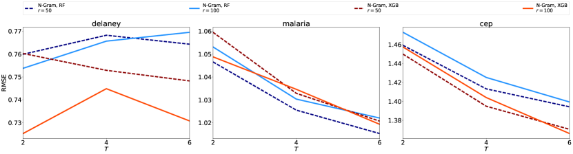
Figure S2: Effects of vertex embedding dimension $r$ and N-gram dimension $T$ on tasks Delaney, Malaria and CEP: how the RMSE on validation set changes as different $r$ and $T$.

Appendix L Exploring the Effects of Atom Features

To further prove that different atom features are not biasing the graph neural networks, we compare the different atom attribute schemes. In N-Gram graph, we are using Table S5 (called new attribute scheme), while in the benchmark paper [56], it has more atom symbols, and may not include attributes like “is acceptor” or “is donor” (called original attribute scheme). We did a statistical test to measure the difference from two atom attribute schemes as in Table S19.

Table S19: For each message-passing graph method, we compare the performance on 12 Tox21 tasks. The null hypothesis here is that means are the same, so rejection=False means we should accept the null hypothesis. Thus, this table shows that two attribute schemes contain very similar information with respect to the performance.

Group 1	Group 2	mean diff	reject
GCNN new attribute scheme	GCNN original attribute scheme	-0.0012	False
Weave new attribute scheme	Weave original attribute scheme	0.0008	False

References

- [1] Aids antiviral screen data. https://wiki.nci.nih.gov/display/NCIDTPdata/AIDS+Antiviral+Screen+Data. Accessed: 2017-09-27.
- [2] Han Altae-Tran, Bharath Ramsundar, Aneesh S Pappu, and Vijay Pande. Low data drug discovery with one-shot learning. ACS Central Science, 3(4):283–293, 2017.
- [3] Sanjeev Arora, Mikhail Khodak, Nikunj Saunshi, and Kiran Vodrahalli. A compressed sensing view of unsupervised text embeddings, bag-of-n-grams, and lstm. International Conference on Learning Representations, 2018.
- [4] Sanjeev Arora, Yuanzhi Li, Yingyu Liang, Tengyu Ma, and Andrej Risteski. A latent variable model approach to pmi-based word embeddings. Transactions of the Association for Computational Linguistics, 4:385–399, 2016.
- [5] Sanjeev Arora, Yuanzhi Li, Yingyu Liang, Tengyu Ma, and Andrej Risteski. Linear algebraic structure of word senses, with applications to polysemy. Transactions of the Association of Computational Linguistics, 6:483–495, 2018.
- [6] Sanjeev Arora, Yingyu Liang, and Tengyu Ma. A simple but tough-to-beat baseline for sentence embeddings. In International Conference on Learning Representations, 2016.
- [7] Artem V Artemov, Evgeny Putin, Quentin Vanhaelen, Alexander Aliper, Ivan V Ozerov, and Alex Zhavoronkov. Integrated deep learned transcriptomic and structure-based predictor of clinical trials outcomes. bioRxiv, page 095653, 2016.
- [8] Lorenz C Blum and Jean-Louis Reymond. 970 million druglike small molecules for virtual screening in the chemical universe database gdb-13. Journal of the American Chemical Society, 131(25):8732–8733, 2009.
- [9] Keith T Butler, Daniel W Davies, Hugh Cartwright, Olexandr Isayev, and Aron Walsh. Machine learning for molecular and materials science. Nature, 559(7715):547, 2018.
- [10] Robert Calderbank, Sina Jafarpour, and Robert Schapire. Compressed learning: Universal sparse dimensionality reduction and learning in the measurement domain. Techical Report, 2009.
- [11] Diogo M Camacho, Katherine M Collins, Rani K Powers, James C Costello, and James J Collins. Next-generation machine learning for biological networks. Cell, 2018.
- [12] Emmanuel J Candes. The restricted isometry property and its implications for compressed sensing. Comptes rendus mathematique, 346(9-10):589–592, 2008.
- [13] Emmanuel J CANDES and Terence TAO. Decoding by linear programming. IEEE transactions on information theory, 51(12):4203–4215, 2005.
- [14] Hongming Chen, Ola Engkvist, Yinhai Wang, Marcus Olivecrona, and Thomas Blaschke. The rise of deep learning in drug discovery. Drug discovery today, 2018.
- [15] Tianqi Chen and Carlos Guestrin. Xgboost: A scalable tree boosting system. In Proceedings of the 22Nd ACM SIGKDD International Conference on Knowledge Discovery and Data Mining, pages 785–794. ACM, 2016.
- [16] Travers Ching, Daniel S Himmelstein, Brett K Beaulieu-Jones, Alexandr A Kalinin, Brian T Do, Gregory P Way, Enrico Ferrero, Paul-Michael Agapow, Michael Zietz, Michael M Hoffman, et al. Opportunities and obstacles for deep learning in biology and medicine. Journal of The Royal Society Interface, 15(141):20170387, 2018.
- [17] George Dahl. Deep learning how i did it: Merck 1st place interview. Online article available from http://blog. kaggle. com/2012/11/01/deep-learning-how-i-did-it-merck-1st-place-interview, 2012.
- [18] John S. Delaney. ESOL: Estimating Aqueous Solubility Directly from Molecular Structure. Journal of Chemical Information and Computer Sciences, 44(3):1000–1005, May 2004.
- [19] David K Duvenaud, Dougal Maclaurin, Jorge Iparraguirre, Rafael Bombarell, Timothy Hirzel, Alan Aspuru-Guzik, and Ryan P Adams. Convolutional Networks on Graphs for Learning Molecular Fingerprints. pages 2224–2232, 2015.
- [20] Felix A Faber, Luke Hutchison, Bing Huang, Justin Gilmer, Samuel S Schoenholz, George E Dahl, Oriol Vinyals, Steven Kearnes, Patrick F Riley, and O Anatole von Lilienfeld. Prediction errors of molecular machine learning models lower than hybrid dft error. Journal of chemical theory and computation, 13(11):5255–5264, 2017.
- [21] Matthias Fey and Jan E. Lenssen. Fast graph representation learning with PyTorch Geometric. In ICLR Workshop on Representation Learning on Graphs and Manifolds, 2019.
- [22] Simon Foucart and Holger Rauhut. A mathematical introduction to compressive sensing. Bull. Am. Math, 54:151–165, 2017.
- [23] Francisco-Javier Gamo, Laura M. Sanz, Jaume Vidal, Cristina de Cozar, Emilio Alvarez, Jose-Luis Lavandera, Dana E. Vanderwall, Darren V. S. Green, Vinod Kumar, Samiul Hasan, James R. Brown, Catherine E. Peishoff, Lon R. Cardon, and Jose F. Garcia-Bustos. Thousands of chemical starting points for antimalarial lead identification. Nature, 465(7296):305–310, May 2010.
- [24] Kaitlyn M Gayvert, Neel S Madhukar, and Olivier Elemento. A data-driven approach to predicting successes and failures of clinical trials. Cell chemical biology, 23(10):1294–1301, 2016.
- [25] Justin Gilmer, Samuel S. Schoenholz, Patrick F. Riley, Oriol Vinyals, and George E. Dahl. Neural message passing for quantum chemistry. In Doina Precup and Yee Whye Teh, editors, Proceedings of the 34th International Conference on Machine Learning, volume 70 of Proceedings of Machine Learning Research, pages 1263–1272, International Convention Centre, Sydney, Australia, 06–11 Aug 2017. PMLR.
- [26] Justin Gilmer, Samuel S Schoenholz, Patrick F Riley, Oriol Vinyals, and George E Dahl. Neural message passing for quantum chemistry. In Proceedings of the 34th International Conference on Machine Learning-Volume 70, pages 1263–1272. JMLR. org, 2017.
- [27] Rafael Gómez-Bombarelli, Jennifer N Wei, David Duvenaud, José Miguel Hernández-Lobato, Benjamín Sánchez-Lengeling, Dennis Sheberla, Jorge Aguilera-Iparraguirre, Timothy D Hirzel, Ryan P Adams, and Alán Aspuru-Guzik. Automatic chemical design using a data-driven continuous representation of molecules. ACS Central Science, 2016.
- [28] Aditya Grover and Jure Leskovec. node2vec: Scalable feature learning for networks. In Proceedings of the 22nd ACM SIGKDD international conference on Knowledge discovery and data mining, pages 855–864. ACM, 2016.
- [29] Johannes Hachmann, Roberto Olivares-Amaya, Sule Atahan-Evrenk, Carlos Amador-Bedolla, Roel S. Sánchez-Carrera, Aryeh Gold-Parker, Leslie Vogt, Anna M. Brockway, and Alán Aspuru-Guzik. The Harvard Clean Energy Project: Large-Scale Computational Screening and Design of Organic Photovoltaics on the World Community Grid. The Journal of Physical Chemistry Letters, 2(17):2241–2251, September 2011.
- [30] William L Hamilton, Rex Ying, and Jure Leskovec. Representation learning on graphs: Methods and applications. arXiv preprint arXiv:1709.05584, 2017.
- [31] Stanisław Jastrzębski, Damian Leśniak, and Wojciech Marian Czarnecki. Learning to smile (s). arXiv preprint arXiv:1602.06289, 2016.
- [32] Shiva Prasad Kasiviswanathan and Mark Rudelson. Restricted isometry property under high correlations. arXiv preprint arXiv:1904.05510, 2019.
- [33] Steven Kearnes, Kevin McCloskey, Marc Berndl, Vijay Pande, and Patrick Riley. Molecular graph convolutions: moving beyond fingerprints. Journal of computer-aided molecular design, 30(8):595–608, 2016.
- [34] Matt J Kusner, Brooks Paige, and José Miguel Hernández-Lobato. Grammar variational autoencoder. arXiv preprint arXiv:1703.01925, 2017.
- [35] Greg Landrum. Rdkit: Open-source cheminformatics software. 2016.
- [36] Yujia Li, Daniel Tarlow, Marc Brockschmidt, and Richard Zemel. Gated graph sequence neural networks. arXiv preprint arXiv:1511.05493, 2015.
- [37] Shengchao Liu, Moayad Alnammi, Spencer S Ericksen, Andrew F Voter, James L Keck, F Michael Hoffmann, Scott A Wildman, and Anthony Gitter. Practical model selection for prospective virtual screening. bioRxiv, page 337956, 2018.
- [38] Junshui Ma, Robert P Sheridan, Andy Liaw, George E Dahl, and Vladimir Svetnik. Deep neural nets as a method for quantitative structure–activity relationships. Journal of chemical information and modeling, 55(2):263–274, 2015.
- [39] Matthew K. Matlock, Na Le Dang, and S. Joshua Swamidass. Learning a Local-Variable Model of Aromatic and Conjugated Systems. ACS Central Science, 4(1):52–62, January 2018.
- [40] Merck. Merck molecular activity challenge. https://www.kaggle.com/c/MerckActivity, 2012.
- [41] Tomas Mikolov, Ilya Sutskever, Kai Chen, Greg S Corrado, and Jeff Dean. Distributed representations of words and phrases and their compositionality. In Advances in neural information processing systems, pages 3111–3119, 2013.
- [42] HL Morgan. The generation of a unique machine description for chemical structures-a technique developed at chemical abstracts service. Journal of Chemical Documentation, 5(2):107–113, 1965.
- [43] Raghunathan Ramakrishnan, Mia Hartmann, Enrico Tapavicza, and O Anatole Von Lilienfeld. Electronic spectra from tddft and machine learning in chemical space. The Journal of chemical physics, 143(8):084111, 2015.
- [44] Bharath Ramsundar, Peter Eastman, Patrick Walters, Vijay Pande, Karl Leswing, and Zhenqin Wu. Deep Learning for the Life Sciences. O’Reilly Media, 2019. https://www.amazon.com/Deep-Learning-Life-Sciences-Microscopy/dp/1492039837.
- [45] Sebastian G Rohrer and Knut Baumann. Maximum unbiased validation (muv) data sets for virtual screening based on pubchem bioactivity data. Journal of chemical information and modeling, 49(2):169–184, 2009.
- [46] Lars Ruddigkeit, Ruud Van Deursen, Lorenz C Blum, and Jean-Louis Reymond. Enumeration of 166 billion organic small molecules in the chemical universe database gdb-17. Journal of chemical information and modeling, 52(11):2864–2875, 2012.
- [47] Kristof T Schütt, Farhad Arbabzadah, Stefan Chmiela, Klaus R Müller, and Alexandre Tkatchenko. Quantum-chemical insights from deep tensor neural networks. Nature communications, 8:13890, 2017.
- [48] John Shawe-Taylor, Nello Cristianini, et al. Kernel methods for pattern analysis. Cambridge university press, 2004.
- [49] Nino Shervashidze, Pascal Schweitzer, Erik Jan van Leeuwen, Kurt Mehlhorn, and Karsten M Borgwardt. Weisfeiler-lehman graph kernels. Journal of Machine Learning Research, 12(Sep):2539–2561, 2011.
- [50] Roberto Todeschini and Viviana Consonni. Molecular descriptors for chemoinformatics: volume I: alphabetical listing/volume II: appendices, references, volume 41. John Wiley & Sons, 2009.
- [51] Tox21 Data Challenge. Tox21 data challenge 2014. https://tripod.nih.gov/tox21/challenge/, 2014.
- [52] Thomas Unterthiner, Andreas Mayr, Günter Klambauer, Marvin Steijaert, Jörg K Wegner, Hugo Ceulemans, and Sepp Hochreiter. Deep learning as an opportunity in virtual screening. Advances in neural information processing systems, 27, 2014.
- [53] Sida Wang and Christopher D Manning. Baselines and bigrams: Simple, good sentiment and topic classification. In Proceedings of the 50th Annual Meeting of the Association for Computational Linguistics: Short Papers-Volume 2, pages 90–94. Association for Computational Linguistics, 2012.
- [54] David Weininger, Arthur Weininger, and Joseph L Weininger. Smiles. 2. algorithm for generation of unique smiles notation. Journal of Chemical Information and Computer Sciences, 29(2):97–101, 1989.
- [55] John Wieting, Mohit Bansal, Kevin Gimpel, and Karen Livescu. Towards universal paraphrastic sentence embeddings. arXiv preprint arXiv:1511.08198, 2015.
- [56] Zhenqin Wu, Bharath Ramsundar, Evan N Feinberg, Joseph Gomes, Caleb Geniesse, Aneesh S Pappu, Karl Leswing, and Vijay Pande. Moleculenet: a benchmark for molecular machine learning. Chemical Science, 9(2):513–530, 2018.
- [57] Zonghan Wu, Shirui Pan, Fengwen Chen, Guodong Long, Chengqi Zhang, and Philip S Yu. A comprehensive survey on graph neural networks. arXiv preprint arXiv:1901.00596, 2019.
- [58] Keyulu Xu, Weihua Hu, Jure Leskovec, and Stefanie Jegelka. How powerful are graph neural networks? arXiv preprint arXiv:1810.00826, 2018.
- [59] Zi Yin and Yuanyuan Shen. On the dimensionality of word embedding. In Advances in Neural Information Processing Systems, pages 895–906, 2018.
- [60] Rex Ying, Jiaxuan You, Christopher Morris, Xiang Ren, William L Hamilton, and Jure Leskovec. Hierarchical graph representation learning withdifferentiable pooling. arXiv preprint arXiv:1806.08804, 2018.
- [61] Jie Zhou, Ganqu Cui, Zhengyan Zhang, Cheng Yang, Zhiyuan Liu, and Maosong Sun. Graph neural networks: A review of methods and applications. arXiv preprint arXiv:1812.08434, 2018.