Exponentially convergent symbolic algorithm of the functional-discrete method for the fourth order Sturm–Liouville problems with polynomial coefficients

Abstract

A new symbolic algorithmic implementation of the functional-discrete (FD-) method is developed and justified for the solution of fourth order Sturm–Liouville problem on a finite interval in the Hilbert space. The eigenvalue problem for the fourth order ordinary differential equation with polynomial coefficients is investigated. The sufficient conditions of an exponential convergence rate of the proposed approach are received. The obtained estimates of the absolute errors of FD-method significantly improve the accuracy of the estimates obtained earlier by I.P Gavrilyuk, V.L. Makarov and A.M. Popov in 2010. Our algorithm is symbolic and operates with the decomposition coefficients of the eigenfunction corrections in some basis. The number of summands in these decompositions depends on the degree of the potential coefficients and the correction number. Our method uses only the algebraic operations and basic operations on $(2\times 1)$ column vectors and $(2\times 2)$ matrices. The proposed approach does not require solving any boundary value problems and computations of any integrals, unlike the previous variants of FD-method by I.P. Gavrilyuk, V.L. Makarov, A.M. Popov and N.M. Romaniuk in 2010 and 2017. The corrections to eigenpairs are computed exactly as analytical expressions, and there are no rounding errors. The numerical examples illustrate the theoretical results. The numerical results obtained with the FD-method are compared with the numerical test results obtained with other existing numerical techniques.

1 Introduction

There is a great number of numerical methods for Sturm–Liouville problems for the second- and higher-order ordinary differential equations. The analytical methods based on perturbation and homotopy ideas [1, 2] are widely used for solving the eigenvalue problems. The numerical-analytical (functional-discrete) methods refer to these methods (see, for example, [3, 4, 5, 6, 7, 8, 9, 10] and compare with Adomian decomposition method [11, 12]). Using these analytical methods the solutions can be found as fast convergent functional series. The properties of the solution of the original problem can be investigated with the help of approximation solution. Moreover, these approaches allow in a natural way to use computer algebra systems for developing and implementation of symbolic-numerical algorithms.

The functional-discrete (FD-) method was suggested by V. Makarov [3] in 1991. In subsequent years, FD-method was developed for the solution of many different problems. This method enables us to overcome many disadvantages of the discrete methods such as:

1. the accuracy degradation with the increasing of the eigenvalue index;

2. usage of the mesh generated at the start of the numerical process;

3. saturation of accuracy;

4. the number of reliable numerical eigenvalues is limited and depends on a mesh step (see [13, 14]).

The main advantages of FD-method are its features, which differ from many other methods:

1. the approach can be applied to operator equations in general form;

2. the approach can be applied also to eigenvalue problems with multiple eigenvalues (see, for example, [10]);

3. all eigenpairs can be computed in parallel;

4. the convergence rate increases as the index of the eigenpair increases;

5. it was proved that in many cases the FD-method converges exponentially or super-exponentially.

Presented modification of the traditional algorithm of the functional-discrete (FD-) method was proposed in [4]. The general idea of the symbolic algorithms for FD-method is the representation of the eigenfunction corrections in some basis. Then we obtain recurrence relations for the decomposition coefficients. Finally, our algorithm operates with these decomposition coefficients. The modified FD-method does not require solving any boundary value problems and computations of any integrals. In certain cases, the algorithm uses only the algebraic operations. Moreover, the corrections to eigenpairs are computed exactly as analytical expressions, and there are no rounding errors. But if computational difficulties or memory overflow arise then we can avoid combinatorial explosion. In proposed approach instead of using rational arithmetic we can easily transit to floating–point arithmetic which ”represents an alternative idea: round the computation at every step, not just at the end” (see [15]).

Briefly described general idea was used for developing and justification of new symbolic algorithms for FD-method for the Sturm–Liouville problems on a finite interval for the Schrödinger equation with a polynomial potential in [6, 8]. Using the described idea for the fourth order Sturm–Liouville problem, in this article we modify the traditional method from [5, 10] and develop a new symbolic algorithm of the FD-method. The proposed algorithm of our method is developed when the potential coefficients are approximated by zero function. For this case, FD-method is purely analytical method and may be considered one of the variants of the homotopy method [1, 2]. Note that some of the results of this article were announced in [7]. Unlike the symbolic algorithm in [7], the presented approach produces explicit recursive formulas for the decomposition coefficients of the representation for the eigenfunctions corrections.

The article is organized as follows. Section 2 deals with the problem statement. Section 3 contains the traditional algorithm of the simplest variant of the FD-method. In Section 4 a new structural representation of the eigenfunctions corrections is obtained. This representation is used in Section 6 to develop a new symbolic algorithm of the FD-method. The sufficient conditions of an exponential convergence rate and the absolute errors estimates of the proposed approach are received in Section 5. The obtained absolute errors estimates of the FD-method significantly improve the accuracy of the estimates obtained earlier in [5]. Derivation of the basic formulas for the proposed new symbolic algorithmic implementation of our method is given in Section 6 and in Appendices A, B, C. The numerical algorithm is given in Section 7. Section 8 illustrates the theoretical results by numerical examples. In Examples 1 and 2 the numerical results obtained with the FD-method are compared with the numerical test results obtained with other existing numerical techniques [16, 17, 18, 19, 20, 21]. A review of the obtained results with implementation features and advantages of our developed numerical method are given in the final Section 9.

2 Problem statement

Let us consider the regular Sturm–Liouville problem in a Hilbert space for the fourth order ordinary differential equation

$$u^{{\rm IV}}(x)+q_{2}(x)u^{\prime\prime}(x)+q_{1}(x)u^{\prime}(x)+\left(q_{0}(x)-\lambda\right)u(x)=0,$$ (1)

$$x\in{\kern 1.0pt}(0,X),\;\;0<X<\infty,$$

with the boundary conditions

$$u(0)=u^{\prime\prime}(0)=u(X)=u^{\prime\prime}(X)=0,$$ (2)

where $X$ is the real constant. The real-valued polynomial coefficients are

$$q_{0}(x)=\sum_{l=0}^{r_{0}}A_{l}x^{l},\;\;q_{1}(x)=\sum_{l=0}^{r_{1}}B_{l}x^{l},\;\;q_{2}(x)=\sum_{l=0}^{r_{2}}C_{l}x^{l},\;\;r_{i}\geq 1,i=0,1,2,$$ (3)

where the constants $r_{i}$, $i=0,1,2$ are positive integers, and $q_{i}(x)\in C^{i}[0,X]$, $i=0,1,2$.

In [5] it was shown that the fourth order ordinary differential equation with all derivatives of the eigenfunction could be reduced to the form (1) using the variable transformation. That is why we consider the eigenvalue problem with equation (1).

3 Traditional algorithm of the simplest variant of the FD-method

In this article, the simplest variant of the FD-method is applied to the Sturm–Liouville problem (1)–(3). It means that we consider the simplest case of the approximation of potential coefficients (3) by zero function

$$\bar{q}_{s}(x)\equiv 0,\;\;\;s=0,1,2.$$

This section contains the traditional algorithm of the FD-method which in this case is the purely analytical method. In this case, FD-method can be considered as one of the variants of the homotopy method (see [1, 2]), and its idea is closely related to the ideas of the Adomian decomposition method [11, 12]. Below the symbolic algorithm for the simplest variant of the FD-method is developed.

Note that in the case when the simplest variant of the FD-method (with $\bar{q}_{s}(x)\equiv 0$, $s=0,1,2$) is divergent for the smallest eigenvalues of the problem (1)–(3), the general scheme of the FD-method (usually) with piecewise-constant approximations to potential coefficients is used. Developing and justification of a symbolic algorithmic implementation of the general scheme of the FD-method for the problem (1)–(3) are slated for the near future.

The exact solution of the eigenvalue problem (1)–(3) is then represented by the series

$$u_{n}(x)=\sum_{j=0}^{\infty}u_{n}^{(j)}(x),{\kern 1.0pt}\;\;\;\lambda_{n}=\sum_{j=0}^{\infty}\lambda_{n}^{(j)},$$ (4)

provided that these series converge. The sufficient conditions for the convergence of the series (4) will be presented later in Section 5. The approximate solution to the problem (1)–(3) is represented by a pair of corresponding truncated series, namely,

$$\mathop{u_{n}}\limits^{m}(x)=\sum_{j=0}^{m}\;u_{n}^{(j)}(x),{\kern 1.0pt}\;\;\;\mathop{\lambda_{n}}\limits^{m}=\sum_{j=0}^{m}\;\lambda_{n}^{(j)},$$ (5)

which is called an approximation of rank $m$ to eigenpair (eigenfunction $u_{n}(x)$ and eigenvalue $\lambda_{n}$) with index number $n$. The summands of series (5) $u_{n}^{(j)}(x)$, $\lambda_{n}^{(j)}$ are called the corrections to eigenpairs at the $j$–th step of the FD-method. The corrections $u_{n}^{(j+1)}(x)$, $\lambda_{n}^{(j+1)}$ are the solutions of the following recursive sequence of problems (see [5])

$$\frac{d^{4}}{dx^{4}}u_{n}^{(j+1)}(x)-\lambda_{n}^{(0)}u_{n}^{(j+1)}(x)=F_{n}^{(j+1)}(x),\;\;\;x\in(0,X),$$ (6)

$$u_{n}^{(j+1)}(0)=\frac{d^{2}u_{n}^{(j+1)}(0)}{dx}=u_{n}^{(j+1)}(X)=\frac{d^{2}u_{n}^{(j+1)}(X)}{dx}=0,\;$$ (7)

$$j=0,1,...,m-1,$$

where

$$\begin{split}F_{n}^{(j+1)}(x)&=\sum_{p=0}^{j}\lambda_{n}^{(j+1-p)}u_{n}^{(p)}(x)-q_{2}(x)\frac{d^{2}}{dx^{2}}u_{n}^{(j)}(x)\\ &-q_{1}(x)\frac{d}{dx}u_{n}^{(j)}(x)-q_{0}(x)u_{n}^{(j)}(x).\end{split}$$ (8)

Using the solvability condition

$$\left(F_{n}^{(j+1)}(x),u_{n}^{(0)}(x)\right)_{L_{2}\left(0,X\right)}=\int_{0}^{X}F_{n}^{(j+1)}(x)u_{n}^{(0)}(x)dx=0$$ (9)

of problems (6)–(8) for a fixed $j$ $(j=0,1,...)$, we obtain the following formula for the eigenvalue corrections:

$$\lambda_{n}^{(j+1)}=\int_{0}^{X}\left(q_{2}(x)\frac{d^{2}}{dx^{2}}u_{n}^{(j)}(x)+q_{1}(x)\frac{d}{dx}u_{n}^{(j)}(x)+q_{0}(x)u_{n}^{(j)}(x)\right)u_{n}^{(0)}(x)dx.$$ (10)

Solutions to the problems (6)–(8) satisfy the orthogonality condition

$$\left(u_{n}^{(j+1)}(x),u_{n}^{(0)}(x)\right)_{L_{2}\left(0,X\right)}=\int_{0}^{X}u_{n}^{(j+1)}(x)u_{n}^{(0)}(x)dx=0,$$ (11)

$$j=0,1,...,m-1.$$

The initial approximation $u_{n}^{(0)}(x)$, $\lambda_{n}^{(0)}$ is the solution of the so-called base problem, that is,

$$\frac{d^{4}u_{n}^{(0)}(x)}{dx^{4}}-\lambda_{n}^{(0)}u_{n}^{(0)}(x)=0,\;\;x\in(0,X),$$ (12)

$$u_{n}^{(0)}(0)=\frac{d^{2}u_{n}^{(0)}(0)}{dx}=u_{n}^{(0)}(X)=\frac{d^{2}u_{n}^{(0)}(X)}{dx}=0.$$ (13)

The solution of (12)–(13) is the following

$$u_{n}^{(0)}(x)=\sqrt{\frac{2}{X}}\sin\left(\frac{n\pi}{X}x\right),\;\;\lambda_{n}^{(0)}=\frac{\left(n\pi\right)^{4}}{X^{4}}.$$ (14)

4 Representation of the corrections to eigenfunctions $u_{n}^{(j)}(x)$

Let us introduce the generalized Green’s function for a linear differential operator, corresponding to the problems by (6)–(14), in the following form

$$g_{n}(x,\xi)=\frac{2X^{3}}{\pi^{4}}\sum_{p=1,p\neq n}^{\infty}\frac{\sin\left(\frac{p\pi}{X}x\right)\sin\left(\frac{p\pi}{X}\xi\right)}{p^{4}-n^{4}},\;\;x,\xi\in\left[0,X\right].$$ (15)

The function (15) can be expressed as

$$\begin{split}g_{n}(x,\xi)&=\frac{X^{3}}{2\pi^{3}n^{3}}\left[-\left(\frac{x}{X}-{\rm H}\left(\frac{x-\xi}{X}\right)\right)\cos\left(\frac{n\pi}{X}x\right)\right.\sin\left(\frac{n\pi}{X}\xi\right)\\ &-\left(\frac{\xi}{X}-{\rm H}\left(\frac{\xi-x}{X}\right)\right)\sin\left(\frac{n\pi}{X}x\right)\cos\left(\frac{n\pi}{X}\xi\right)+\\ &+\frac{1}{\sinh\left(\pi n\right)}\sinh\left(\pi n\left(\frac{x}{X}-{\rm H}\left(\frac{x-\xi}{X}\right)\right)\right)\\ &\times\sinh\left(\pi n\left(\frac{\xi}{X}-{\rm H}\left(\frac{\xi-x}{X}\right)\right)\right)\left.+\frac{3}{2\pi n}\sin\left(\frac{n\pi}{X}x\right)\sin\left(\frac{n\pi}{X}\xi\right)\right],\end{split}$$ (16)

$$x,\xi\in\left[0,X\right],$$

where ${\rm H}(x)$ is the Heaviside function, and ${\rm H}(0)=1$.

Lemma 1

The generalized Green’s function (15), (16) has the following properties:

$$g_{n}(x,\xi)=g_{n}(\xi,x),\;\;\;\;\;g_{n}(x,\xi)=g_{n}(X-x,X-\xi),$$

$$\int_{0}^{X}g_{n}(x,\xi)\sin\left(\frac{\pi n}{X}x\right)dx=0.$$

For a fixed $j$ the solution of a problem (6)–(9), (3), which satisfies the orthogonality condition (11), can be expressed by a formula

$$u_{n}^{(j+1)}(x)=\int_{0}^{X}g_{n}(x,\xi)F_{n}^{(j+1)}(\xi)d\xi.$$ (17)

The following assertion is proved by a method of complete induction. To accomplish this we use the integral representation (17) and the solution of the base problem (14), as well as the properties of the problems (6)–(9), (3) and of the generalized Green’s function (15), (16) (see Lemma 1).

Lemma 2

The solution of problem (6)–(9), (3) can be represented by

$$\begin{split}u_{n}^{(j+1)}(x)&=\sum_{p=0}^{M(j+1)}x^{p}\left[b_{n,p}^{(j+1)}\cos\left(\frac{\pi n}{X}x\right)+a_{n,p}^{(j+1)}\sin\left(\frac{\pi n}{X}x\right)\right]\\ &+\sum_{p=0}^{M(j)}x^{p}\left[d_{n,p}^{(j+1)}\cosh\left(\frac{\pi n}{X}x\right)+c_{n,p}^{(j+1)}\sinh\left(\frac{\pi n}{X}x\right)\right],\\ &j=0,1,...,\;n=1,2,...\end{split}$$ (18)

where $M(j)=j(r+1)$, $r=\max\left\{r_{0},r_{1},r_{2}\right\},$ $a_{n,0}^{(0)}=\sqrt{\frac{2}{X}}$, $b_{n,0}^{(0)}=d_{n,0}^{(0)}=c_{n,0}^{(0)}=0$.

In Lemma 2 the coefficients

$$\begin{split}&b_{p}^{(j+1)},\;\;a_{p}^{(j+1)}\;\;(p=0,1,...,M(j+1)),\\ &c_{s}^{(j+1)},\;\;d_{s}^{(j+1)}\;\;(s=0,1,...,M(j))\end{split}$$ (19)

are the decomposition coefficients of the eigenfunction corrections $u_{n}^{(j+1)}(x)$ in the basis

$$x^{p}\cos\left(\frac{\pi n}{X}x\right),\;\;x^{p}\sin\left(\frac{\pi n}{X}x\right)\;\;(p=0,1,...,M(j+1)),$$

$$x^{s}\cosh\left(\frac{\pi n}{X}x\right),\;\;x^{s}\sinh\left(\frac{\pi n}{X}x\right)\;\;(s=0,1,...,M(j))$$

on interval $\left[0,X\right]$. Unlike (17), the representation (18) is used below to develop a new symbolic algorithmic implementation of the FD-method, numerical algorithm for which is fully given in Section 7. Exact explicit recursive formulas for these coefficients are found in Section 6 (see (55), (56), (57) and (58)).

5 Convergence of the FD-method

To investigate the convergence of the FD-method we substitute the expressions (10) and (17) into formulas

$$\begin{split}\lambda_{n}^{(j+1)}&=\sqrt{\frac{2}{X}}\int_{0}^{X}\left(-\left(\frac{n\pi}{X}\right)^{2}\right.q_{2}(x)\sin\left(\frac{n\pi}{X}x\right)\\ &+\frac{n\pi}{X}\left[2q^{\prime}_{2}(x)-q_{1}(x)\right]\cos\left(\frac{n\pi}{X}x\right)\\ &+\left[q^{\prime\prime}_{2}(x)-q^{\prime}_{1}(x)+q_{0}(x)\right]\left.\sin\left(\frac{n\pi}{X}x\right)\right)u_{n}^{(j)}(x)dx\end{split}$$ (20)

and

$$\begin{split}u_{n}^{(j+1)}&(x)=\frac{2X^{3}}{\pi^{4}}\sum_{p=1,p\neq n}^{\infty}\frac{1}{p^{4}-n^{4}}\sin\left(\frac{p\pi}{X}x\right)\\ &\times\int_{0}^{X}\left\{\left[\left(\frac{p\pi}{X}\right)^{2}q_{2}(\xi)\sin\left(\frac{p\pi}{X}\xi\right)\right.\right.\\ &+\frac{p\pi}{X}\left[-2q^{\prime}_{2}(\xi)+q_{1}(\xi)\right]\cos\left(\frac{p\pi}{X}\xi\right)\\ &+\left[-q^{\prime\prime}_{2}(\xi)+q^{\prime}_{1}(\xi)-q_{0}(\xi)\right]\left.\sin\left(\frac{p\pi}{X}\xi\right)\right]u_{n}^{(j)}(\xi)\\ &+\left.\sum_{s=0}^{j}\;\lambda_{n}^{(j+1-s)}u_{n}^{(s)}(\xi)\sin\left(\frac{p\pi}{X}\xi\right)\right\}d\xi.\end{split}$$ (21)

The formulas (20) and (21) were obtained using the integration by parts as well as the representation for the generalized Green’s function $g_{n}(x,\xi)$ by a series (15). Note that obtained in this Section absolute errors estimates of the FD-method significantly improve the accuracy of the estimates obtained earlier in [5].

One can deduce from (20) the next estimate for the eigenvalue corrections

$$\left|\lambda_{n}^{(j+1)}\right|\leq\omega\sqrt{\frac{2}{X}}\left[\left(\frac{n\pi}{X}\right)^{2}+\frac{n\pi}{X}+1\right]\left\|u_{n}^{(j)}\right\|,$$ (22)

where

$$\omega=\max\left\{\left\|q_{2}\right\|_{\infty},\left\|2q^{\prime}_{2}-q_{1}\right\|_{\infty},\left\|q^{\prime\prime}_{2}-q^{\prime}_{1}+q_{0}\right\|_{\infty}\right\},\;\;\;\;\left\|v\right\|_{\infty}=\mathop{\max}\limits_{x\in[0,X]}\left|v(x)\right|,$$

$$\left\|v\right\|=\sqrt{\left(v(x),v(x)\right)_{L_{2}\left(0,X\right)}}=\left(\int_{0}^{X}\;\left[v(x)\right]^{2}dx\right)^{{}^{{1\mathord{\left/{\vphantom{12}}\right.\kern-1.2pt}2}}}.$$

It is easy to establish that the following inequalities are correct:

$$\sqrt{\sum_{p=1,p\neq n}^{\infty}\frac{p^{4-2k}}{\left(p^{4}-n^{4}\right)^{2}}}\leq\frac{n^{1-k}}{2n^{2}-2n+1},\,k=0,1,2,\,n=1,2,...$$

which are used to obtain from (22) the estimate for the eigenfunction corrections (21):

$$\begin{split}&\left\|u_{n}^{(j+1)}\right\|\leq\frac{X^{2}}{\pi^{2}}\frac{1}{2n^{2}-2n+1}\left[\left[n\left\|q_{2}\right\|_{\infty}+\frac{X}{\pi}\left\|-2q^{\prime}_{2}+q_{1}\right\|_{\infty}\right.\right.\\ &\left.+\frac{X^{2}}{\pi^{2}}\frac{\left\|-q^{\prime\prime}_{2}+q^{\prime}_{1}-q_{0}\right\|_{\infty}}{n}\right]\left\|u_{n}^{(j)}\right\|+\sqrt{\frac{2}{X}}\omega\left[n+\frac{X}{\pi}+\frac{X^{2}}{n\pi^{2}}\right]\\ &\times\left.\sum_{s=0}^{j}\;\left\|u_{n}^{(j-s)}\right\|\left\|u_{n}^{(s)}\right\|\right]\leq\frac{X^{2}}{\pi^{2}}\frac{\omega}{2n^{2}-2n+1}\left[n+\frac{X}{\pi}+\frac{X^{2}}{n\pi^{2}}\right]\\ &\times\left[\left\|u_{n}^{(j)}\right\|+\sqrt{\frac{2}{X}}\sum_{s=0}^{j}\;\left\|u_{n}^{(j-s)}\right\|\left\|u_{n}^{(s)}\right\|\right]\leq M_{n}\sum_{s=0}^{j}\;\left\|u_{n}^{(j-s)}\right\|\left\|u_{n}^{(s)}\right\|,\end{split}$$ (23)

where

$$M_{n}=\frac{X^{2}}{\pi^{2}}\frac{\omega}{2n^{2}-2n+1}\left[n+\frac{X}{\pi}+\frac{X^{2}}{n\pi^{2}}\right]\max\left\{1,\sqrt{\frac{2}{X}}\right\}.$$ (24)

Substituting in (23)

$$U_{j}=M_{n}^{-j}\left\|u_{n}^{\left(j\right)}\right\|,\;\;\;\;U_{0}=\left\|u_{n}^{\left(0\right)}\right\|=1$$ (25)

and replacing the new variables by the majorant variables subject to

$$U_{j}\leq\overline{U}_{j},\;\;\;\;\overline{U}_{0}=U_{0}=1,$$

we come to the majorant equation

$$\overline{U}_{j+1}=\sum_{s=0}^{j}\overline{U}_{j-s}\overline{U}_{s}.$$ (26)

This equation is the nonlinear recurrence relation and the so-called convolution-type equation. The solution of the equation (26) is (see, e.g., [22, p. 159-161,210], [23])

$$\overline{U}_{j+1}=\frac{\left(2j+2\right)!}{\left(j+1\right)!\left(j+2\right)!}=4^{j+1}2\frac{\left(2j+1\right)!!}{\left(2j+4\right)!!}.$$ (27)

Returning to the old variables (see substitution of variables (25)), we obtain from (27) the following estimate for the solution of (23):

$$\left\|u_{n}^{\left(j+1\right)}\right\|\leq\left(4M_{n}\right)^{j+1}2\frac{\left(2j+1\right)!!}{\left(2j+4\right)!!}\leq\frac{\left(4M_{n}\right)^{j+1}}{\left(j+2\right)\sqrt{\pi\left(j+1\right)}},$$ (28)

and then, from (22), the next estimate for the eigenvalue corrections

$$\begin{split}\left|\lambda_{n}^{(j+1)}\right|&\leq\omega\sqrt{\frac{2}{X}}\left[\left(\frac{n\pi}{X}\right)^{2}+\frac{n\pi}{X}+1\right]\left(4M_{n}\right)^{j}2\frac{\left(2j-1\right)!!}{\left(2j+2\right)!!}\\ &\leq\omega\sqrt{\frac{2}{X}}\left[\left(\frac{n\pi}{X}\right)^{2}+\frac{n\pi}{X}+1\right]\frac{\left(4M_{n}\right)^{j}}{\left(j+1\right)\sqrt{\pi j}}.\end{split}$$ (29)

The last parts of inequalities (28) and (29) were obtained using the judgements like those from the proof of the Wallis formula (see, e.g., [24, p. 344]). From estimates (28) and (29) follows the next theorem which contains the sufficient conditions of an exponential convergence rate of the FD-method and estimates of its absolute errors.

Theorem 1

Let $q_{i}(x)\in C^{i}[0,X]$, $i=0,1,2$ and let the following condition hold true:

$$r_{n}=4M_{n}<1,n=1,2,....$$ (30)

Then the FD-method for the Sturm–Liouville problem (1)–(3) converges exponentially and the following estimates of the absolute errors are valid:

$$\left|\lambda_{n}-\mathop{\lambda_{n}}\limits^{m}\right|\leq\omega\sqrt{\frac{2}{X}}\left[\left(\frac{n\pi}{X}\right)^{2}+\frac{n\pi}{X}+1\right]\frac{\left(r_{n}\right)^{m}}{1-r_{n}}\frac{1}{\left(m+1\right)\sqrt{\pi m}},$$ (31)

$$\left\|u_{n}-\mathop{u_{n}}\limits^{m}\right\|\leq 2\frac{\left(r_{n}\right)^{m+1}}{1-r_{n}}\frac{\left(2m+1\right)!!}{\left(2m+4\right)!!}\leq\frac{\left(r_{n}\right)^{m+1}}{\left(m+2\right)\sqrt{\pi\left(m+1\right)}}.$$ (32)

6 Derivation of basic formulas for the symbolic algorithm of the FD-method

Further, in this section, we describe and develop a new symbolic algorithm of the FD-method for the problem (1)–(3). In this section, basic formulas of the symbolic algorithm are given and also additional formulas are given in Appendices A, B, C. Unlike the symbolic algorithm from [7], the presented approach produces explicit recursive formulas for the coefficients in (18) at the $(j+1)$–th step of the FD-method. Then the computer algebra system Maple was used for a software implementation.

Let us substitute (18) into (8), (3) and group together the summands as follows

$$\begin{split}F_{n}^{(j+1)}(x)&=F_{n,\cos}^{(j+1)}(x)\cos\left(\frac{\pi n}{X}x\right)+F_{n,\sin}^{(j+1)}(x)\sin\left(\frac{\pi n}{X}x\right)\\ &+F_{n,\cosh}^{(j+1)}(x)\cosh\left(\frac{\pi n}{X}x\right)+F_{n,\sinh}^{(j+1)}(x)\sinh\left(\frac{\pi n}{X}x\right)\end{split}$$ (33)

changing the order of summation in analytical expressions for $F_{n,\cos}^{(j+1)}(x)$, $F_{n,\sin}^{(j+1)}(x)$, $F_{n,\cosh}^{(j+1)}(x)$ and $F_{n,\sinh}^{(j+1)}(x)$ (see Appendix A). Then we group together the summands as follows

$$\begin{split}F_{n}^{(j+1)}(x)&=\sum_{p=0}^{M(j+1)-1}x^{p}\left(f_{n,\cos,p}^{(j+1)}\cos\left(\frac{\pi n}{X}x\right)+f_{n,\sin,p}^{(j+1)}\sin\left(\frac{\pi n}{X}x\right)\right)\\ &+\sum_{p=0}^{M(j)-1}x^{p}\left(f_{n,\cosh,p}^{(j+1)}\cosh\left(\frac{\pi n}{X}x\right)+f_{n,\sinh,p}^{(j+1)}\sinh\left(\frac{\pi n}{X}x\right)\right).\end{split}$$ (34)

To extract the coefficients of $x^{p}$ like

$$f_{n,\cos,p}^{(j+1)},\;f_{n,\sin,p}^{(j+1)},\;p=0,1,...,M(j+1)-1$$

and

$$f_{n,\cosh,p}^{(j+1)},\;f_{n,\sinh,p}^{(j+1)},\;p=0,1,...,M(j)-1$$

in the polynomials $F_{n,\cos}^{(j+1)}(x)$, $F_{n,\sin}^{(j+1)}(x)$, $F_{n,\cosh}^{(j+1)}(x)$, $F_{n,\sinh}^{(j+1)}(x)$ (see Appendix A) noted above, we can use the function coeff with corresponding arguments in Maple. These coefficients are included in the main formulas of the proposed algorithm in Section 7. The expressions for these coefficients involve only the algebraic operations and are represented through the corresponding quantities computed at previous steps of FD-method.

We require the polynomials at corresponding trigonometric functions and hyperbolic trigonometric functions to be equal on the both sides of equation (6), (34). This requirement leads to the two recurrence systems (35), (36) (with the initial conditions (37), (38)) and (39), (40) (with the initial conditions (41), (42)) for the unknown coefficients of representation (18).

The first system is the following:

$$\begin{split}\left(\left(\left((t+4)b_{n,t+4}^{(j+1)}+4\frac{\pi n}{X}a_{n,t+3}^{(j+1)}\right)(t+3)-6\left(\frac{\pi n}{X}\right)^{2}b_{n,t+2}^{(j+1)}\right)(t+2)\right.&\\ \left.-4\left(\frac{\pi n}{X}\right)^{3}a_{n,t+1}^{(j+1)}\right)(t+1)=f_{n,\cos,t}^{(j+1)},&\end{split}$$ (35)

$$\begin{split}\left(\left(\left((t+4)a_{n,t+4}^{(j+1)}-4\frac{\pi n}{X}b_{n,t+3}^{(j+1)}\right)(t+3)-6\left(\frac{\pi n}{X}\right)^{2}a_{n,t+2}^{(j+1)}\right)(t+2)\right.&\\ \left.+4\left(\frac{\pi n}{X}\right)^{3}b_{n,t+1}^{(j+1)}\right)(t+1)=f_{n,\sin,t}^{(j+1)},&\end{split}$$ (36)

$$t=0,1,...,M\left(j+1\right)-4,\;\;\;\;\;j=0,1,2,...$$

with the initial conditions

$$\begin{split}a_{n,M(j+1)-s}^{(j+1)}&=\sum_{k=0}^{s}(-1)^{\left[\kern-1.04996pt\left[\left.\left.\frac{k}{2}\right]\kern-1.04996pt\right]\right.\right.+1}f_{n,\chi(k),M(j+1)-s-1+k}^{(j+1)}\\ &\times\frac{(2k+1)(M(j+1)-1)^{k}}{2^{2+k}\left(M(j+1)-s+\left[\kern-3.50006pt\left[\left.\left.\frac{k+\delta_{2,s}}{2}\right]\kern-3.50006pt\right]\right.\right.\right)}\left(\frac{X}{\pi n}\right)^{3+k},\end{split}$$ (37)

$$\begin{split}b_{n,M(j+1)-s}^{(j+1)}&=\sum_{k=0}^{s}(-1)^{\left[\kern-1.04996pt\left[\left.\left.\frac{k+1}{2}\right]\kern-1.04996pt\right]\right.\right.}f_{n,\chi(k+1),M(j+1)-s-1+k}^{(j+1)}\\ &\times\frac{(2k+1)(M(j+1)-1)^{k}}{2^{2+k}\left(M(j+1)-s+\left[\kern-3.50006pt\left[\left.\left.\frac{k+\delta_{2,s}}{2}\right]\kern-3.50006pt\right]\right.\right.\right)}\left(\frac{X}{\pi n}\right)^{3+k},\end{split}$$ (38)

where $s=0,1,2$, $\chi(2p)=\cos$, $\chi(2p+1)=\sin$, $p=0,1$, $j=0,1,2,...$. Here and below $\delta_{t,s}$ denotes the Kronecker delta, $\left[\kern-1.49994pt\left[y\right]\kern-1.49994pt\right]$ is the greatest integer less than or equal to a real number $y$ (in the computer algebra system Maple $\left[\kern-1.49994pt\left[y\right]\kern-1.49994pt\right]$ is the function floor(y)).

The second system is the following:

$$\begin{split}\left(\left(\left((t+4)d_{n,t+4}^{(j+1)}+4\frac{\pi n}{X}c_{n,t+3}^{(j+1)}\right)(t+3)+6\left(\frac{\pi n}{X}\right)^{2}d_{n,t+2}^{(j+1)}\right)(t+2)\right.&\\ \left.+4\left(\frac{\pi n}{X}\right)^{3}c_{n,t+1}^{(j+1)}\right)(t+1)=f_{n,\cosh,t}^{(j+1)},&\end{split}$$ (39)

$$\begin{split}\left(\left(\left((t+4)c_{n,t+4}^{(j+1)}+4\frac{\pi n}{X}d_{n,t+3}^{(j+1)}\right)(t+3)+6\left(\frac{\pi n}{X}\right)^{2}c_{n,t+2}^{(j+1)}\right)(t+2)\right.&\\ \left.+4\left(\frac{\pi n}{X}\right)^{3}d_{n,t+1}^{(j+1)}\right)(t+1)=f_{n,\sinh,t}^{(j+1)},&\end{split}$$ (40)

$$t=0,1,...,M(j)-4,\;\;\;\;\;j=1,2,...$$

with the initial conditions

$$\begin{split}c_{n,M(j)-s}^{(j+1)}&=\sum_{k=0}^{s}(-1)^{\left[\kern-1.04996pt\left[\frac{k+1}{2}\right]\kern-1.04996pt\right]}f_{n,\chi h(k),M(j)-s-1+k}^{(j+1)}\\ &\times\frac{(2k+1)(M(j)-1)^{k}}{2^{2+k}\left(M(j)-s+\left[\kern-3.50006pt\left[\left.\left.\frac{k+\delta_{2,s}}{2}\right]\kern-3.50006pt\right]\right.\right.\right)}\left(\frac{X}{\pi n}\right)^{3+k},\end{split}$$ (41)

$$\begin{split}d_{n,M(j)-s}^{(j+1)}&=\sum_{k=0}^{s}(-1)^{\left[\kern-1.04996pt\left[\frac{k+1}{2}\right]\kern-1.04996pt\right]}f_{n,\chi h(k+1),M(j)-s-1+k}^{(j+1)}\\ &\times\frac{(2k+1)(M(j)-1)^{k}}{2^{2+k}\left(M(j)-s+\left[\kern-3.50006pt\left[\left.\left.\frac{k+\delta_{2,s}}{2}\right]\kern-3.50006pt\right]\right.\right.\right)}\left(\frac{X}{\pi n}\right)^{3+k},\end{split}$$ (42)

where $s=0,1,2$, $\chi h(2p)=\cosh$, $\chi h(2p+1)=\sinh$, $p=0,1$, $j=1,2,...$.

Let us introduce the column vectors:

$$\begin{split}\vec{Z}_{n}^{[a,b]}(p,j)&=\left[a_{n,M(j+1)-p}^{(j+1)},b_{n,M(j+1)-p}^{(j+1)}\right]^{T},\\ \vec{F}_{n}^{[a,b]}(p+3,j)&=\frac{1}{4(M(j+1)-p-3)}\left(\frac{X}{\pi n}\right)^{3}\\ &\times\left[-f_{n,\cos,M(j+1)-p-4}^{(j+1)},f_{n,\sin,M(j+1)-p-4}^{(j+1)}\right]^{T},\end{split}$$ (43)

$$\begin{split}\vec{Z}_{n}^{[c,d]}(s,j)&=\left[c_{n,M(j)-s}^{(j+1)},d_{n,M(j)-s}^{(j+1)}\right]^{T},\\ \vec{F}_{n}^{[c,d]}(s+3,j)&=\frac{1}{4(M(j)-s-3)}\left(\frac{X}{\pi n}\right)^{3}\\ &\times\left[f_{n,\cosh,M(j)-s-4}^{(j+1)},f_{n,\sinh,M(j)-s-4}^{(j+1)}\right]^{T},\end{split}$$ (44)

and denote the matrices:

$$\begin{split}D_{n,1,1}^{[a,b]}(p,j)&=\frac{3X}{2\pi n}(M(j+1)-p-2)\left[\begin{array}[]{cc}{0}&{-1}\\ {1}&{0}\end{array}\right],\\ D_{n,1,2}^{[a,b]}(p,j)&=\left(\frac{X}{\pi n}\right)^{2}(M(j+1)-p-1)(M(j+1)-p-2)\left[\begin{array}[]{cc}{1}&{0}\\ {0}&{1}\end{array}\right],\\ D_{n,1,3}^{[a,b]}(p,j)&=-\frac{1}{4}\left(\frac{X}{\pi n}\right)^{3}(M(j+1)-p)(M(j+1)-p-1)\\ \end{split}$$ (45)

$$\begin{split}&\times(M(j+1)-p-2)\left[\begin{array}[]{cc}{0}&{-1}\\ {1}&{0}\end{array}\right]\end{split}$$

for $j=0,1,...$, and

$$\begin{split}&D_{n,1,1}^{[c,d]}(s,j)=\left[\begin{array}[]{cc}{1}&{0}\\ {0}&{-1}\end{array}\right]D_{1,1}^{[a,b]}(s,j-1),\\ &D_{n,1,2}^{[c,d]}(s,j)=-D_{1,2}^{[a,b]}(s,j-1),\\ &D_{n,1,3}^{[c,d]}(s,j)=-\left[\begin{array}[]{cc}{1}&{0}\\ {0}&{-1}\end{array}\right]D_{1,3}^{[a,b]}(s,j-1)\end{split}$$ (46)

for $j=1,2,...$. Here by $T$ we denote the transpose of a row vector. For some fixed $j$ the systems of equations (35)–(38) and (39)–(42) can be expressed in vector form as linear inhomogeneous third-order difference equations with variable matrix coefficients

$$\begin{split}\vec{Z}_{n}^{\nu}(p+3,j)&=D_{n,1,1}^{\nu}(p,j)\vec{Z}_{n}^{\nu}(p+2,j)+D_{n,1,2}^{\nu}(p,j)\vec{Z}_{n}^{\nu}(p+1,j)\\ &+D_{n,1,3}^{\nu}(p,j)\vec{Z}_{n}^{\nu}(p,j)+\vec{F}_{n}^{\nu}(p+3,j),\end{split}$$ (47)

where

$$p=0,1,...,M\left(j+1\right)-4,\;\;\;j=0,1,...\;\;\;\text{with}\;\;\;\nu=[a,b]$$

and

$$p=0,1,...,M\left(j\right)-4,\;\;\;j=1,2,...\;\;\;\text{with}\;\;\;\nu=[c,d],$$

with the initial value vectors (see (37), (38) and (41), (42))

$$\vec{Z}_{n}^{\nu}(k,j),\;\;k=0,1,2,\;\;\;\nu=[a,b],\,[c,d].$$ (48)

Let us define the column vectors

$$\begin{split}\mathbf{Z}_{n}^{\nu}(p,j)&=\left[\vec{Z}_{n}^{\nu}(p+2,j),\vec{Z}_{n}^{\nu}(p+1,j),\vec{Z}_{n}^{\nu}(p,j)\right]^{T},\\ \mathbf{F}_{n}^{\nu}(p)&=\left[\vec{F}_{n}^{\nu}(p+3,j),\vec{0},\vec{0}\right]^{T},\end{split}$$ (49)

and the block matrix

$$\begin{split}\mathbf{D}_{n}^{\nu}(p,j)&=\left[\begin{array}[]{ccc}{D_{n,1,1}^{\nu}(p,j)}&{D_{n,1,2}^{\nu}(p,j)}&{D_{n,1,3}^{\nu}(p,j)}\\ {E}&{O}&{O}\\ {O}&{E}&{O}\end{array}\right]\\ &=\left(D_{n,l_{1},l_{2}}^{\nu}(p,j)\right)_{l_{1},l_{2}=\overline{1,3}}\end{split}$$ (50)

with

$$\begin{split}D_{n,2,1}^{\nu}(p,j)&=D_{n,3,2}^{\nu}(p,j)=E,\\ D_{n,2,2}^{\nu}(p,j)&=D_{n,2,3}^{\nu}(p,j)=D_{n,3,1}^{\nu}(p,j)=D_{n,3,3}^{\nu}(p,j)=O.\end{split}$$ (51)

Here $E$ and $O$ are respectively the unit and zero $(2\times 2)$–matrices, $\vec{0}=\left[0,0\right]^{T}$ is the null column vector. We can rewrite (47), (48) as

$$\begin{split}&\mathbf{Z}_{n}^{\nu}(p+1,j)=\mathbf{D}_{n}^{\nu}(p,j)\mathbf{Z}_{n}^{\nu}(p,j)+\mathbf{F}_{n}^{\nu}(p,j),\\ &\mathbf{Z}_{n}^{\nu}(0,j)=\left[\vec{Z}_{n}^{\nu}(2,j),\vec{Z}_{n}^{\nu}(1,j),\vec{Z}_{n}^{\nu}(0,j)\right]^{T},\end{split}$$ (52)

where

$$p=0,1,...,M\left(j+1\right)-4,\;\;\;j=0,1,...\;\;\;\text{with}\;\;\;\nu=[a,b]$$

and

$$p=0,1,...,M\left(j\right)-4,\;\;\;j=1,2,...\;\;\;\text{with}\;\;\;\nu=[c,d].$$

The solution of (52) can then be given in matrix form by

$$\begin{split}&\mathbf{Z}_{n}^{\nu}(p+1,j)=\mathbf{D}_{n}^{\nu}(p,j)\mathbf{D}_{n}^{\nu}(p-1,j)\cdot\ldots\cdot\mathbf{D}_{n}^{\nu}(0,j)\mathbf{Z}_{n}^{\nu}(0,j)+\\ &+\sum_{s=1}^{p}\mathbf{D}_{n}^{\nu}(p,j)\mathbf{D}_{n}^{\nu}(p-1,j)\cdot\ldots\cdot\mathbf{D}_{n}^{\nu}(p-s+1,j)\mathbf{F}_{n}^{\nu}(p-s,j)+\mathbf{F}_{n}^{\nu}(p,j).\end{split}$$ (53)

Hence the solution of (47) is

$$\begin{split}&\vec{Z}_{n}^{\nu}(p+3,j)=\sum_{\begin{subarray}{l}{1\leq l_{p},l_{p-1},...,l_{0}\leq 3,}\\ {l_{p+1}=1}\end{subarray}}\prod_{s=0}^{p}D_{n,l_{s+1},l_{s}}^{\nu}(s,j)\vec{Z}_{n}^{\nu}(3-l_{0},j)\\ &+\sum_{s=1}^{p}\sum_{\begin{subarray}{l}{1\leq l_{s-1},...,l_{1}\leq 3,}\\ {l_{0}=1,\;l_{s}=1}\end{subarray}}\prod_{k=1}^{s}D_{n,l_{k},l_{k-1}}^{\nu}(p-s+k,j)\vec{F}_{n}^{\nu}(p-s+3,j)\\ &+\vec{F}_{n}^{\nu}(p+3,j),\end{split}$$ (54)

where

$$p=0,1,...,M\left(j+1\right)-4,\;\;\;j=0,1,...\;\;\;\text{with}\;\;\;\nu=[a,b]$$

and

$$p=0,1,...,M\left(j\right)-4,\;\;\;j=1,2,...\;\;\;\text{with}\;\;\;\nu=[c,d].$$

Remark 1

Note, if the upper bound of summation index is less than the lower bound of summation index, then the sum is the empty sum, with the value $0$. In (54) and below in (55), (56) we multiply the matrices $D_{n,l_{s+1},l_{s}}^{\nu}(s,j)$ from the right to the left, i.e.,

$$\begin{split}&\prod_{s=0}^{p}D_{n,l_{s+1},l_{s}}^{\nu}(s,j)\vec{Z}_{n}^{\nu}(3-l_{0},j)\\ &=D_{n,1,l_{p}}^{\nu}(p,j)\cdot\left(D_{n,l_{p},l_{p-1}}^{\nu}(p-1,j)\cdot\right.\left(\ldots\right.\\ &\ldots\left.\left.\cdot\left(D_{n,l_{2},l_{1}}^{\nu}(1,j)\left(D_{n,l_{1},l_{0}}^{\nu}(0,j)\vec{Z}_{n}^{\nu}(3-l_{0},j)\right)\right)\cdots\right)\right).\end{split}$$

In (54) and below in (55), (56) the notation

$$\sum_{\begin{subarray}{l}{\;\;\;1\leq l_{p},l_{p-1},...,l_{0}\leq 3,}\\ {\,\,\,\,\,\,l_{p+1}=1}\end{subarray}}$$

denotes the following expression

$$\sum_{l_{p+1}=1}^{1}\sum_{l_{p}=1}^{3}\sum_{l_{p-1}=1}^{3}\cdots\sum_{l_{2}=1}^{3}\sum_{l_{1}=1}^{3}\sum_{l_{0}=1}^{3}.$$

Returning to the substitution (43), (44), from (54) we obtain the following column vectors:

$$\begin{split}&\left[\!\!\begin{array}[]{l}{a_{n,M(j+1)-p-3}^{(j+1)}}\\ {b_{n,M(j+1)-p-3}^{(j+1)}}\end{array}\!\!\right]\!\!=\!\sum_{\begin{subarray}{l}{1\leq l_{p},l_{p-1},...,l_{0}\leq 3,}\\ {l_{p+1}=1}\end{subarray}}\prod_{s=0}^{p}\!D_{n,l_{s+1},l_{s}}^{[a,b]}(s,j)\!\!\left[\!\!\begin{array}[]{l}{a_{n,M(j+1)-3+l_{0}}^{(j+1)}}\\ {b_{n,M(j+1)-3+l_{0}}^{(j+1)}}\end{array}\!\!\right]\\ &+\frac{1}{4}\left(\frac{X}{\pi n}\right)^{3}\sum_{s=1}^{p}\frac{1}{M(j+1)+s-p-3}\\ &\times\sum_{\begin{subarray}{l}{1\leq l_{s-1},...,l_{1}\leq 3,}\\ {l_{0}=1,\,\,l_{s}=1}\end{subarray}}\prod_{k=1}^{s}\!D_{n,l_{k},l_{k-1}}^{[a,b]}(p-s+k,j)\!\left[\!\begin{array}[]{l}{-f_{n,\cos,M(j+1)-p+s-4}^{(j+1)}}\\ {f_{n,\sin,M(j+1)-p+s-4}^{(j+1)}}\end{array}\!\right]\\ &+\frac{1}{4(M(j+1)-p-3)}\left(\frac{X}{\pi n}\right)^{3}\left[\begin{array}[]{l}{-f_{n,\cos,M(j+1)-p-4}^{(j+1)}}\\ {f_{n,\sin,M(j+1)-p-4}^{(j+1)}}\end{array}\right],\end{split}$$ (55)

$$p=0,1,...,M\left(j+1\right)-4,\;\;\;j=0,1,2,...$$

and

$$\begin{split}&\left[\begin{array}[]{l}{c_{n,M(j)-p-3}^{(j+1)}}\\ {d_{n,M(j)-p-3}^{(j+1)}}\end{array}\right]=\sum_{\begin{subarray}{l}{1\leq l_{p},l_{p-1},...,l_{0}\leq 3,}\\ {l_{p+1}=1}\end{subarray}}\prod_{s=0}^{p}D_{n,l_{s+1},l_{s}}^{[c,d]}(s,j)\left[\begin{array}[]{l}{c_{n,M(j)-3+l_{0}}^{(j+1)}}\\ {d_{n,M(j)-3+l_{0}}^{(j+1)}}\end{array}\right]\\ &+\frac{1}{4}\left(\frac{X}{\pi n}\right)^{3}\sum_{s=1}^{p}\frac{1}{4(M(j)+s-p-3)}\\ &\times\sum_{\begin{subarray}{l}{1\leq l_{s-1},...,l_{1}\leq 3,}\\ {l_{0}=1,\,\,l_{s}=1}\end{subarray}}\prod_{k=1}^{s}D_{n,l_{k},l_{k-1}}^{[c,d]}(p-s+k,j)\;\left[\begin{array}[]{l}{f_{n,\cosh,M(j)-p+s-4}^{(j+1)}}\\ {f_{n,\sinh,M(j)-p+s-4}^{(j+1)}}\end{array}\right]\\ &+\frac{1}{4(M(j)-p-3)}\left(\frac{X}{\pi n}\right)^{3}\left[\begin{array}[]{l}{f_{n,\cosh,M(j)-p-4}^{(j+1)}}\\ {f_{n,\sinh,M(j)-p-4}^{(j+1)}}\end{array}\right],\end{split}$$ (56)

$$p=0,1,...,M\left(j\right)-4,\;\;\;j=1,2,....$$

Namely, we obtain the explicit recursive formulas for the coefficients in (18)

$$a_{n,M(j+1)-p-3}^{(j+1)},\;\;\;\;b_{n,M(j+1)-p-3}^{(j+1)},\;\;\;\;p=0,1,...,M\left(j+1\right)-4,\;\;\;\;j=0,1,2,...$$

and

$$c_{n,M(j)-p-3}^{(j+1)},\;\;\;\;d_{n,M(j)-p-3}^{(j+1)},\;\;\;\;p=0,1,...,M\left(j\right)-4,\;\;\;\;j=1,2,...$$

which are the corresponding elements of the vectors (55) and (56). These coefficients are represented recursively through the corresponding coefficients and quantities computed at previous steps of FD-method as well as through the coefficients of the polynomials (3).

Substituting the representation (18) in the boundary conditions (7), we obtain the nonhomogeneous system of linear algebraic equations for the coefficients $b_{n,0}^{(j+1)}$, $c_{n,0}^{(j+1)}$, $d_{n,0}^{(j+1)}$, $j=0,1,2,...$. The solution of this system is:

$$\begin{split}b_{n,0}^{(j+1)}&=\frac{X}{\pi n}\left(a_{n,1}^{(j+1)}+c_{n,1}^{(j+1)}+\frac{X}{\pi n}\left(b_{n,2}^{(j+1)}+d_{n,2}^{(j+1)}\right)\right),\;c_{n,1}^{(1)}=d_{n,2}^{(1)}=0,\\ d_{n,0}^{(j+1)}&=-b_{n,0}^{(j+1)},\\ c_{n,0}^{(j+1)}\!&=\!-\frac{1}{\sinh\left(\pi n\right)}\left(\!\sum_{t=0}^{M(j+1)}X^{t}b_{n,t}^{(j+1)}\!\cos\left(\pi n\right)+\sum_{t=0}^{M(j)}X^{t}d_{n,t}^{(j+1)}\!\cosh\left(\pi n\right)\!\right)\\ &-\sum_{t=1}^{M(j)}X^{t}c_{n,t}^{(j+1)},\;\;\;j=0,1,2,...\end{split}$$ (57)

The constant $a_{n,0}^{(j+1)}$ is calculated by the formula

$$\begin{split}a_{n,0}^{(j+1)}&=-\frac{2}{X}\left(\sum_{t=1}^{M(j+1)}\left(\beta_{n,t}b_{n,t}^{(j+1)}+\alpha_{n,t}a_{n,t}^{(j+1)}\right)\right.\\ &+\left.\sum_{t=0}^{M(j)}\left(\eta_{n,t}d_{n,t}^{(j+1)}+\mu_{n,t}c_{n,t}^{(j+1)}\right)\right),\;\;\;\;j=0,1,2,...\end{split}$$ (58)

obtained from the orthogonality condition (11) and the formulas (57). Here the notations $\alpha_{n,t}$, $\beta_{n,t}$, $\eta_{n,t}$, $\mu_{n,t}$ are used which are exactly calculated in the case $t=0,1,...$. The analytical expressions for these notations are given in Appendix B (see also [25]).

Using Lemma 2, from (10) we obtain the formula for the corrections of the eigenvalues $\lambda_{n}^{(j+1)}$ which is given in Appendix C.

Remark 2

Analytical expressions for the approximations $\mathop{\lambda_{n}}\limits^{m}$, $\mathop{u_{n}}\limits^{m}(x)$ of rank $m$ (according to the FD-method) to the exact eigenpairs $\lambda_{n}$, $u_{n}(x)$ are the results of the execution of a numerical algorithm from Section 7. These expressions analytically depend on the eigenpair index number $n$ and on the input data of the problem under consideration (1)–(3) as $X$, $r_{0}$, $r_{1}$, $r_{2}$, $A_{l}$ $(l=0,1,...,r_{0})$, $B_{l}$ $(l=0,1,...,r_{1})$, $C_{l}$ $(l=0,1,...,r_{2})$. In order to find numerically result for a given value of $n$, we calculate the corresponding approximations $\mathop{\lambda_{n}}\limits^{m}$, $\mathop{u_{n}}\limits^{m}(x)$, by substituting in the obtained analytical expressions the value $n$ and the numerical values of the parameters entering into the input data, if there are any.

7 Numerical algorithm

Data: choose a set of input values: $X,$ $r_{0},r_{1},r_{2},$ $A_{l}(l=0,1,...,r_{0}),$
$B_{l}(l=0,1,...,r_{1}),$ $C_{l}(l=0,1,...,r_{2})$, $m$ $(m\geq 1)$ (see problem (1)–(3));

Result: $\mathop{\lambda_{n}}\limits^{m}$, $\mathop{u_{n}}\limits^{m}(x)$;

1. set input parameters for a recurrence procedure $r=\max\left\{r_{0},r_{1},r_{2}\right\}$, $a_{n,0}^{(0)}=\sqrt{\frac{2}{X}}$, $b_{n,0}^{(0)}=d_{n,0}^{(0)}=c_{n,0}^{(0)}=0$, $\lambda_{n}^{(0)}=\frac{\left(n\pi\right)^{4}}{X^{4}}$, $u_{n}^{(0)}(x)=a_{n,0}^{(0)}\sin\left(\frac{n\pi}{X}x\right)$;

2. compute the values of ancillary quantities $\beta_{n,t}$, $\alpha_{n,t}$, $\eta_{n,s}$, $\mu_{n,s}$, $(t=0,1,...,M(m)-1$, $s=0,1,...,M(m-1)-1)$ using Appendix B;

3. compute the correction $\lambda_{n}^{(1)}$ given in Appendix C with $j=0$;

4. compute the functions $F_{n,\cos}^{(1)}(x)$, $F_{n,\sin}^{(1)}(x)$ given in Appendix A with $j=0$ and compute the corresponding coefficients $f_{n,\cos,p}^{(1)}$, $f_{n,\sin,p}^{(1)}$ $(p=0,1,...,r)$ (see (34));

5. compute the coefficients $a_{n,r+1-s}^{(1)}$, $b_{n,r+1-s}^{(1)}$ $(s=0,1,2)$ using (37), (38) with $j=0$;

6. using (45), (51) with $j=0$ compute the matrices

   $$D_{n,l_{s+1},l_{s}}^{[a,b]}(s,0)\;\;(l_{s}=1,2,3,\;s=0,1,...,r-3);$$

   $$D_{n,l_{k},l_{k-1}}^{[a,b]}(p-s+k,0)\;\;(l_{k}=1,2,3,\;k=1,2,...,s,\;s=1,2,...,p,$$

   $$p=0,1,...,r-3);$$

7. compute the coefficients $a_{n,r-p-2}^{(1)}$, $b_{n,r-p-2}^{(1)}$ $(p=0,1,...,r-3)$ using (55) with $j=0$;

8. compute the coefficients $b_{n,0}^{(1)}$, $c_{n,0}^{(1)}$, $d_{n,0}^{(1)}$, $a_{n,0}^{(1)}$ using (57), (58) with $j=0$;

9. compute the correction $u_{n}^{(1)}(x)$ using (18) with $j=0$;
   if $m>1$ then

   for $j$ from $1$ (with unit step) to $m-1$ do

10. compute $\lambda_{n}^{(j+1)}$ given in Appendix C;

11. compute the functions $F_{n,\cos}^{(j+1)}(x)$, $F_{n,\sin}^{(j+1)}(x)$, $F_{n,\cosh}^{(j+1)}(x)$, $F_{n,\sinh}^{(j+1)}(x)$ given in Appendix A and compute the corresponding coefficients $f_{n,\cos,p}^{(j+1)}$, $f_{n,\sin,p}^{(j+1)}$ $(p=0,1,...,M(j+1)-1)$ and $f_{n,\cosh,p}^{(j+1)}$, $f_{n,\sinh,p}^{(j+1)}$ $(p=0,1,...,M(j)-1)$ (see (34));

12. compute the coefficients $a_{n,M(j+1)-s}^{(j+1)}$, $b_{n,M(j+1)-s}^{(j+1)}$, $c_{n,M(j)-s}^{(j+1)}$, $d_{n,M(j)-s}^{(j+1)}$ $(s=0,1,2)$ using (37), (38), (41), (42);

13. using (45), (51) compute the matrices

    $$D_{n,l_{s+1},l_{s}}^{[a,b]}(s,j)\;\;(l_{s}=1,2,3,\;s=0,1,...,M(j+1)-4),$$

    $$D_{n,l_{k},l_{k-1}}^{[a,b]}(p-s+k,j)\;\;(l_{k}=1,2,3,\;k=1,2,...,s,\;s=1,2,...,p,$$

    $$p=0,1,...,M(j+1)-4),$$

    $$D_{n,l_{s+1},l_{s}}^{[c,d]}(s,j)\;\;(l_{s}=1,2,3,\;s=0,1,...,M(j)-4),$$

    $$D_{n,l_{k},l_{k-1}}^{[c,d]}(p-s+k,j)\;\;(l_{k}=1,2,3,\;k=1,2,...,s,\;s=1,2,...,p,$$

    $$p=0,1,...,M(j)-4);$$

14. compute the coefficients $a_{n,M(j+1)-p-3}^{(j+1)}$, $b_{n,M(j+1)-p-3}^{(j+1)}$ $(p=0,1,...,M(j+1)-4)$ using (55) and compute the coefficients $c_{n,M(j)-p-3}^{(j+1)}$, $d_{n,M(j)-p-3}^{(j+1)}$ $(p=0,1,...,M(j)-4)$ using (56);

15. compute the coefficients $b_{n,0}^{(j+1)}$, $c_{n,0}^{(j+1)}$, $d_{n,0}^{(j+1)}$, $a_{n,0}^{(j+1)}$ using (57), (58);

16. compute the correction $u_{n}^{(j+1)}(x)$ using (18);

    end for;

    end if;

17. compute the approximations $\mathop{u_{n}}\limits^{m}(x)$, $\mathop{\lambda_{n}}\limits^{m}$ using (5).

8 Numerical examples

Example 1

We consider the eigenvalue problem (1), (2) with $X=5$, and with potential coefficients in (3) equal to

$$q_{0}(x)=0.0001x^{4}-0.02,\;\;\;q_{1}(x)=-0.04x,\;\;\;q_{2}(x)=-0.02x^{2}.$$ (59)

The computations of the exact eigenvalues $\lambda_{n}$ and eigenfunctions $u_{n}(x)$, and of their approximations $\mathop{\lambda_{n}}\limits^{m}$ and $\mathop{u_{n}}\limits^{m}(x)$ obtained by FD-method of rank $m$, have been done with the help of the computer algebra system Maple (Digits=300).

The exact solution of the problem (1), (2), (59) is expressed in terms of confluent hypergeometric Kummer’s functions $M\left(a,b,z\right)$ and $U\left(a,b,z\right)$ (see [26, Chapter 13])

$$\begin{split}u_{n}&(x)\!=\!\frac{xe^{-{x^{2}\mathord{\left/{\vphantom{x^{2}20}}\right.\kern-1.2pt}20}}}{10^{{3\mathord{\left/{\vphantom{34}}\right.\kern-1.2pt}4}}}\!\left(\!C_{1}M\!\left(\frac{3}{4}+\frac{5}{2}\sqrt{\lambda_{n}},\frac{3}{2},\frac{x^{2}}{10}\right)\right.\!+\!C_{2}M\!\left(\frac{3}{4}\!-\!\frac{5}{2}\sqrt{\lambda_{n}},\frac{3}{2},\frac{x^{2}}{10}\right)\\ &+\!C_{3}U\left(\frac{3}{4}\!+\!\frac{5}{2}\sqrt{\lambda_{n}},\frac{3}{2},\frac{x^{2}}{10}\right)\!+\!C_{4}\!\left.U\left(\frac{3}{4}\!-\!\frac{5}{2}\sqrt{\lambda_{n}},\frac{3}{2},\frac{x^{2}}{10}\right)\!\right).\end{split}$$ (60)

The constants $C_{k}$, $k=1,2,3,4$ and the eigenvalues $\lambda_{n}$ of the problem (1), (2), (59) can be found from the system of equations obtained by substituting (60) into the boundary conditions (2) with $X=5$. Setting the determinant of this system equal to zero, we obtain a transcendental equation with respect to $\lambda_{n}$

$$\sqrt{\lambda_{n}}M\left(\frac{3}{4}+\frac{5}{2}\lambda_{n},\frac{3}{2},\frac{5}{2}\right)M\left(\frac{3}{4}-\frac{5}{2}\lambda_{n},\frac{3}{2},\frac{5}{2}\right)=0,\;\;\;\;n=1,2,...\;.$$ (61)

Using the command fsolve in Maple, from (61) we find the first eight smallest exact eigenvalues $\lambda_{n}$, $n=1,2,...,8$ of the problem under consideration, which are given in Table 1.

$n$	$\lambda_{n}$
1	0.2150508643697154969799099152379067104370468531017
2	2.7548099346830341769807978567162582697401440677181
3	13.215351540558178725583135747686922412859870693289
4	40.950819759161479687386430406406575369564981705685
5	99.053478063489519905364004392278295950913079764143
6	204.35573226825688655101487325028333585898058873698
7	377.43042068923559313999045804039609985719687266348
8	642.59086816966269512711767453062929784652398288740

Table 1: Exact eigenvalues $\lambda_{n}$ for $n=1,2,...,8$ of the problem (1), (2), (59) from Example 1.

Moreover, the eigenvalues $\lambda_{n}$ of the given problem (1), (2), (59) are precisely the squares of the corresponding eigenvalues $L_{n}$ of the second-order Sturm–Liouville problem with Dirichlet boundary conditions (see [27, Section 6]):

$$y^{\prime\prime}(x)+\left(L_{n}-0.01x^{2}\right)y(x)=0,\;x\in\;{\kern 1.0pt}(0,5),\;y(0)=y(5)=0.$$ (62)

The exact solution of (62) is

$$y(x)=\frac{xe^{-{x^{2}\mathord{\left/{\vphantom{x^{2}20}}\right.\kern-1.2pt}20}}}{10^{{3\mathord{\left/{\vphantom{34}}\right.\kern-1.2pt}4}}}\left(C_{1}M\left(\frac{3}{4}-\frac{5}{2}L_{n},\frac{3}{2},\frac{1}{10}x^{2}\right)+C_{2}U\left(\frac{3}{4}-\frac{5}{2}L_{n},\frac{3}{2},\frac{1}{10}x^{2}\right)\right).$$ (63)

The constants $C_{1}$, $C_{2}$ and the eigenvalues $L_{n}$ of the problem (62) can be found from the system of equations obtained by substituting (63) into the boundary conditions $y(0)=y(5)=0$. Setting the determinant of this system equal to zero, we obtain a transcendental equation with respect to $L_{n}$

$$M\left(\frac{3}{4}-\frac{5}{2}L_{n},\frac{3}{2},\frac{5}{2}\right)=0,\;\;\;\;n=1,2,...\;.$$ (64)

Exact eigenvalues $L_{n}$ can be found from (64) using the command fsolve in Maple. The squares of the eigenvalues $L_{n}$, i.e. the values $\lambda_{n}=\left(L_{n}\right)^{2}$, are given in Table 1.

Proposed in this paper symbolic algorithm of the FD-method was applied to compute the approximate solution of the problem (1), (2), (59). The approximate eigenpairs $\mathop{u_{n}}\limits^{m}(x)$, $\mathop{\lambda_{n}}\limits^{m}$ were computed exactly as analytical expressions with respect to the index number $n$ and the input data of the problem under consideration, i.e., we had no rounding errors (see Remark 2). Below we give the eigenvalue corrections $\lambda_{n}^{(j+1)}$ for some first iteration steps $j$ of FD-method:

$$\begin{split}\lambda_{n}^{(0)}&=\frac{\left(n\pi\right)^{4}}{625},\lambda_{n}^{(1)}=\frac{\left(n\pi\right)^{2}}{150}+\frac{1}{400}-\frac{1}{16\left(n\pi\right)^{2}}+\frac{3}{32\left(n\pi\right)^{4}},\\ \lambda_{n}^{(2)}&=-\frac{1}{360}+\frac{1}{224\left(n\pi\right)^{2}}-\frac{173}{384\left(n\pi\right)^{4}}+\frac{9075}{3584\left(n\pi\right)^{6}}-\frac{625\coth\left(n\pi\right)}{64\left(n\pi\right)^{7}}\\ &+\frac{28775}{512\left(n\pi\right)^{8}}-\frac{556875}{2048\left(n\pi\right)^{10}}+\frac{804375}{2048\left(n\pi\right)^{12}},\end{split}$$

$$\begin{split}\lambda_{n}^{(3)}&=-\frac{25}{4472832\left(e^{2\pi n}-1\right)^{2}}\left(\left(\frac{11748744}{\left(\pi n\right)^{8}}-\frac{338782925}{\left(\pi n\right)^{12}}\right)\left(e^{4\pi n}+1\right)\right.\\ \end{split}$$

$$\begin{split}&\left.+\left(-\frac{38057488}{\left(\pi n\right)^{8}}+\frac{814065850}{\left(\pi n\right)^{12}}\right)e^{2\pi n}\right)+\frac{625}{3072}\left(\frac{96}{\left(\pi n\right)^{7}}+\frac{400}{\left(\pi n\right)^{9}}\right.\end{split}$$

$$\begin{split}&\left.-\frac{14250}{\left(\pi n\right)^{11}}-\frac{5625}{\left(\pi n\right)^{13}}+\frac{{\rm 1203750}}{\left(\pi n\right)^{15}}\right)\cosh\left(\pi n\right)-\frac{5}{672\left(\pi n\right)^{2}}+\frac{155}{2688\left(\pi n\right)^{4}}\\ &-\frac{51325}{39424\left(\pi n\right)^{6}}+\frac{{\rm 232994375}}{{\rm 315392}\left(\pi n\right)^{10}}-\frac{{\rm 24718046875}}{{\rm 229376}\left(\pi n\right)^{14}}+\frac{{\rm 54692015625}}{{\rm 65536}\left(\pi n\right)^{16}}\\ &-\frac{{\rm 843444140625}}{{\rm 131072}\left(\pi n\right)^{18}}+\frac{{\rm 675516796875}}{{\rm 65536}\left(\pi n\right)^{20}}.\end{split}$$

Here the command combine(,trig) in Maple was used to rewrite the eigenvalue corrections $\lambda_{n}^{(j+1)}$ in a compact form. We give the coefficients of (18) only for first two steps of the FD-method with $j=-1,0$ because they are too large

$$\begin{split}&a_{n,0}^{(0)}=\sqrt{\frac{2}{5}},\;\;\;b_{n,0}^{(0)}=c_{n,0}^{(0)}=d_{n,0}^{(0)}=0\;\text{(step 1)};\\ &b_{n,5}^{(1)}=-\frac{\sqrt{10}}{8000\left(\pi n\right)^{3}},\;\;\;a_{n,4}^{(1)}=\frac{3\sqrt{10}}{640\left(\pi n\right)^{4}},\;\;\;b_{n,3}^{(1)}=\frac{\sqrt{10}}{8\pi n}\left(-\frac{1}{75}+\frac{5}{8\left(\pi n\right)^{4}}\right),\\ &a_{n,5}^{(1)}=b_{n,4}^{(1)}=a_{n,3}^{(1)}=0\;\text{(step 5)};\\ &a_{n,2}^{(1)}=\frac{\sqrt{10}}{16\left(\pi n\right)^{2}}\left(\frac{1}{5}-\frac{75}{8\left(\pi n\right)^{4}}\right),\;\;\;b_{n,1}^{(1)}=\frac{\sqrt{10}}{8\pi n}\left(\frac{1}{3}+\frac{5}{8\left(\pi n\right)^{2}}-\frac{25}{8\left(\pi n\right)^{4}}\right),\\ &b_{n,2}^{(1)}=a_{n,1}^{(1)}=0\;\text{(step 7)};\\ &c_{n,0}^{(1)}=-\frac{125\sqrt{10}\cos\left(\pi n\right)}{16\left(\pi n\right)^{5}\sinh\left(\pi n\right)},\;a_{n,0}^{(1)}\!=\!\frac{5\sqrt{10}}{128\left(\pi n\right)^{2}}\left(\!-\frac{8}{3}\!-\!\frac{7}{\left(\pi n\right)^{2}}\!+\!\frac{125}{\left(\pi n\right)^{4}}\!-\!\frac{525}{\left(\pi n\right)^{6}}\!\right),\\ &b_{n,0}^{(1)}=d_{n,0}^{(1)}=0\;\text{(step 8)}.\end{split}$$

Here in parentheses the step of the numerical algorithm from Section 7 is given on which these coefficients are calculated.

Using the proposed symbolic algorithm of the FD-method of rank $m=0,1,2,...,20$ the approximations $\mathop{\lambda_{n}}\limits^{m}$ to the first eight eigenvalues $\lambda_{n}$ with $n=1,2,...,8$ were calculated by substitution the value of $n$ into the analytical expressions for $\mathop{\lambda_{n}}\limits^{m}$. Figure 1 shows the broken logarithmic line graphs which were created connecting the data points $\left(m;\ln\left(\Delta_{n}^{FD}(m)\right)\right)$ by lines, where $\Delta_{n}^{FD}(m)=|\lambda_{n}-\mathop{\lambda_{n}}\limits^{m}|$ are the absolute errors of the approximations $\mathop{\lambda_{n}}\limits^{m}$ of rank $m$ to the exact eigenvalues $\lambda_{n}$ with the number $n$. Figure 1 illustrates the exponential convergence of the proposed approach for the problem (1), (2), (59). The sufficient convergence condition (30) (with $\omega=0.2$) is fulfilled for $n\geq 3$, but, as we can see in Figure 1, the method converges for $n=1,2$ too, i.e., the conditions of Theorem 1 are rough and can be improved.

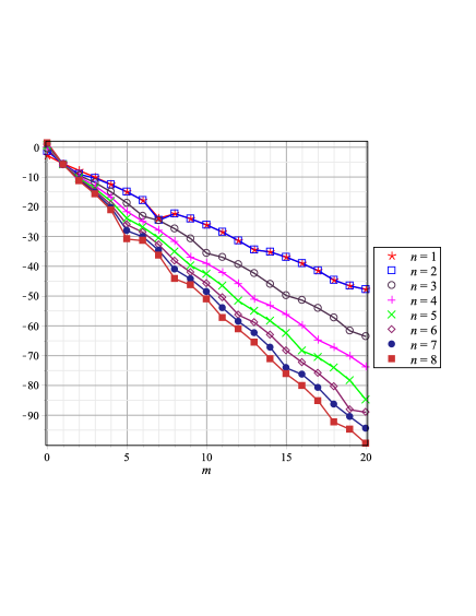
Figure 1: Graphs for broken lines joining the data points $\left(m;\ln\left(\Delta_{n}^{FD}(m)\right)\right)$ for Example 1. These graphs illustrates the behaviour of the absolute errors $\Delta_{n}^{FD}(m)=|\lambda_{n}-\mathop{\lambda_{n}}\limits^{m}|$ of FD-method for $m=0,1,2,...,20$, i.e., they illustrate the exponential convergence of the FD-method with respect to the rank of FD-method $m$ for the eigenpairs $\mathop{u_{n}}\limits^{m}(x)$, $\mathop{\lambda_{n}}\limits^{m}$ with the indices $n=1,2,...8$. Vertical axis $\ln\left(\Delta_{n}^{FD}(m)\right)$, horizontal axis $m$.

This test example (1), (2), (59) was considered in [16, 17, 18, 19, 20] in which the following methods were applied: Adomian decomposition method (ADM) [16], variational iteration method (VIM) [17], homotopy perturbation method (HPM) [18] homotopy analysis method (HAM) [19], extended sampling method (ESM) [20]. Let us compare the behavior of the absolute errors $\Delta_{n}^{FD}(m)$ of FD-method for $m=10,15,20$ with the behavior of the absolute errors $\Delta_{n}^{ADM}$, $\Delta_{n}^{VIM}$, $\Delta_{n}^{HPM}$, $\Delta_{n}^{HAM}$, $\Delta_{n}^{ESM}$ of the corresponding numerical methods from [16, 17, 18, 19, 20] as the index number $n$ of eigenvalue increases. In Table 2 these absolute errors are given. They were calculated using the exact eigenvalues from Table 1 and the approximations from [16, 17, 18, 19, 20].

$n$	$\Delta_{n}^{FD}(10)$	$\Delta_{n}^{FD}(15)$	$\Delta_{n}^{FD}(20)$	$\Delta_{n}^{ADM}$	$\Delta_{n}^{VIM}$	$\Delta_{n}^{HPM}$	$\Delta_{n}^{HAM}$	$\Delta_{n}^{ESM}$
(1)	(2)	(3)	(4)	(5)	(6)	(7)	(8)	(9)
1	4.5e-12	9.0e-17	1.8e-21	4.6e-16	5.8e-16	1.6e-16	4.4e-9	2.8e-13
2	4.5e-12	9.0e-17	1.8e-21	4.9e-14	1.5e-13	1.5e-15	1.1e-6	3.0e-12
3	3.4e-16	2.3e-22	2.4e-28	6.5e-13	6.3e-13	8.5e-13	4.4e-5	4.2e-11
4	1.1e-17	4.1e-25	9.0e-33	2.4e-11	2.4e-11	4.5e-11	2.6e-3	4.1e-7
5	3.1e-19	7.2e-28	1.4e-37	7.5e-8	7.5e-8	2.6e-9	0.35
6	1.3e-20	2.1e-30	2.2e-39	1.2e-3	1.2e-3	1.8e-7	11.4
7	7.8e-22	6.4e-33	9.2e-42	12.7
8	6.6e-23	8.3e-34	5.9e-44	215.5

Table 2: Absolute errors for the first eight eigenvalues $\lambda_{n}$, $n=1,2,...,8$ using the following methods for Example 1 : columns (2), (3), (4) — FD-method for rank $m=10,15,20$ with error $\Delta_{n}^{FD}(m)$; column (5) — ADM with error $\Delta_{n}^{ADM}$ [16]; column (6) — VIM with error $\Delta_{n}^{VIM}$ [17]; column (7) — HPM with error $\Delta_{n}^{HPM}$ [18]; column (8) — HAM with error $\Delta_{n}^{HAM}$ [19]; column (9) — ESM with error $\Delta_{n}^{ESM}$ [20].

One can observe that the convergence rate of each method ADM, VIM, HPM, HAM and ESM rapidly decreases when the eigenvalue index $n$ increases (see columns (5)–(9) in Table 2). The absolute errors $\Delta_{n}^{ADM}$ of the method ADM (variant from [16]) for the 7th and 8th eigenvalues $\lambda_{n}$ with $n=7,8$ are respectively equal to $12.7$ and $215.5$. Moreover the convergence of the FD-method increases together with the index $n$ (see columns (2)–(4) in Table 2) and FD-method converges exponentially with respect to rank $m$ (see Figure 1). The convergence rate is doubled with increase in the rank $m$ (from $10$ to $20$), for example, from $10^{-13}$ (with $m=10$) to $10^{-22}$ (with $m=20$) for $n=1,2$, and from $10^{-24}$ (with $m=10$) to $10^{-45}$ (with $m=20$) for $n=8$.

Example 2

We consider the eigenvalue problem (1), (2) with $X=1$, and with potential coefficients in (3) equal to

$$q_{0}(x)=x,\;\;\;q_{1}(x)=0,\;\;\;q_{2}(x)=0.$$ (65)

Developed new symbolic algorithm of the FD-method (see Section 7) was applied to compute the approximate solution of the problem (1), (2), (65). The approximate eigenpairs $\mathop{u_{n}}\limits^{m}(x)$, $\mathop{\lambda_{n}}\limits^{m}$ were computed exactly as analytical expressions with respect to the index number $n$ and the input data of the problem under consideration, i.e., we had no rounding errors (see Remark 2). Below we give the eigenvalue corrections $\lambda_{n}^{(j+1)}$ for some first iteration steps $j$ of FD-method:

$$\begin{split}&\lambda_{n}^{(0)}=\left(n\pi\right)^{4},\;\lambda_{n}^{(1)}=\frac{1}{2},\\ &\lambda_{n}^{(2)}=\frac{1}{32\left(n\pi\right)^{4}}-\frac{5}{32\left(n\pi\right)^{6}}+\frac{\cos\left(\pi n\right)-\cosh\left(\pi n\right)}{2\left(n\pi\right)^{7}\sinh\left(\pi n\right)},\\ &\lambda_{n}^{(3)}=0,\\ &\lambda_{n}^{(4)}=\frac{11}{20480\left(n\pi\right)^{12}}-\frac{65}{2048\left(n\pi\right)^{14}}-\frac{63e^{2\pi n}-26\cos\left(\pi n\right)e^{\pi n}+63}{128\left(n\pi\right)^{15}\left(e^{2\pi n}-1\right)}\\ &+\frac{8269e^{2\pi n}+16858\cos\left(\pi n\right)e^{\pi n}+8269}{4096\left(n\pi\right)^{16}\left(e^{2\pi n}+2\cos\left(\pi n\right)e^{\pi n}+1\right)}\\ &-\frac{5\cos\left(\pi n\right)e^{3\pi n}+3e^{2\pi n}-3\cos\left(\pi n\right)e^{\pi n}-5}{16\left(n\pi\right)^{17}\left(\cos\left(\pi n\right)e^{3\pi n}+3e^{2\pi n}+3\cos\left(\pi n\right)e^{\pi n}+1\right)}\\ &-\frac{17\left(e^{2\pi n}-2\cos\left(\pi n\right)e^{\pi n}+1\right)}{32\left(n\pi\right)^{18}\left(e^{2\pi n}+2\cos\left(\pi n\right)e^{\pi n}+1\right)}.\end{split}$$

Here the command combine(,trig) in Maple was used to rewrite the eigenvalue corrections $\lambda_{n}^{(j+1)}$ in a compact form. The expressions for the eigenfunctions corrections are too cumbersome. Therefore we give the coefficients of (18) only for first two iteration steps of the FD-method with $j=-1,0$:

$$\begin{split}&a_{0}^{(0)}=\sqrt{2},\;b_{0}^{(0)}=d_{0}^{(0)}=c_{0}^{(0)}=0,\\ &b_{0}^{(1)}=\frac{\sqrt{2}}{4\left(\pi n\right)^{5}},\;b_{1}^{(1)}=\frac{\sqrt{2}}{8\left(\pi n\right)^{3}},\;b_{2}^{(1)}=-\frac{\sqrt{2}}{8\left(\pi n\right)^{3}},\\ &a_{0}^{(1)}=-\frac{3\sqrt{2}}{16\left(\pi n\right)^{4}},\;a_{1}^{(1)}=\frac{3\sqrt{2}}{8\left(\pi n\right)^{4}},\;a_{2}^{(1)}=0,\\ &d_{0}^{(1)}=-\frac{\sqrt{2}}{4\left(\pi n\right)^{5}},\;c_{0}^{(1)}=-\frac{\sqrt{2}\left(\cos\left(\pi n\right)-\cosh\left(\pi n\right)\right)}{4\left(\pi n\right)^{5}\sinh\left(\pi n\right)}.\end{split}$$

It should be noted that in this case, the following properties are satisfied for eigenfunction corrections:

• if the eigenpair index number $n$ is even, then $u_{n}^{(2j+1)}(1-x)=-u_{n}^{(2j+1)}(x)$, $u_{n}^{(2j)}(1-x)=u_{n}^{(2j)}(x)$;

• if the eigenpair index number $n$ is odd, then $u_{n}^{(2j+1)}(1-x)=u_{n}^{(2j+1)}(x)$, $u_{n}^{(2j)}(1-x)=-u_{n}^{(2j)}(x)$.

These properties together with (10), (11) and Lemma 1 imply that at the odd-numbered iteration steps $j$ of the FD-method the corrections to the eigenvalues are zero, i. e., $\lambda_{n}^{(2j+1)}=0$, $j=1,2,...$.

In Table 3 the approximations $\mathop{\lambda_{n}}\limits^{10}$ of rank $m=10$ to the exact eigenvalues $\lambda_{n}$ with $n=1,2,3,4,5,10,20,50$ and the norms of the corresponding residuals are given by

$$\delta_{n}\left(m\right)=\left\|\varphi_{n}^{(m)}(x)\right\|=\left\{\int_{0}^{1}[\varphi_{n}^{(m)}(x)]^{2}dx\right\}^{1/2}$$ (66)

with

$$\varphi_{n}^{(m)}(x)=\frac{d^{4}\mathop{u_{n}}\limits^{m}(x)}{dx^{4}}+(x-\mathop{\lambda_{n}}\limits^{m})\mathop{u_{n}}\limits^{m}(x).$$

They are calculated according to the proposed FD-method of rank $m=10$ with the help of the computer algebra system Maple (Digits=300). Figure 2 shows graphs of the approximations $\mathop{u_{n}}\limits^{10}(x)$ to eigenfunctions $u_{n}(x)$ with $n=1,2,3,4,5$.

According to Theorem 1 the sufficient convergence condition (30) is fulfilled for the eigenpairs with the index $n\geq 2$. For $n=1$ the FD-method can be divergent. However, as can be seen in Table 4 and in Figure 3, the FD-method converges for $n=1$ too. This means that the conditions of Theorem 1 can be improved. Figure 3 shows the broken line graphs which were created connecting the data points $\left(m;\ln\left(\delta_{n}(m)\right)\right)$ by lines (see notation (66)). Figure 3 and Table 4 illustrate the behaviour of the norms of the corresponding residuals $\delta_{n}(m)$ with respect to the rank of FD-method $m$ $(m=1,2,...,10)$ for the indices $n=1,2,3,4,5,10,20,50$, i.e., they illustrate the exponential convergence of the proposed approach for the problem (1), (2), (65). One can observe that the convergence rate of our method increases together with the index $n$ of the eigenpair $\mathop{u_{n}}\limits^{m}(x)$, $\mathop{\lambda_{n}}\limits^{m}$.

$n$	$\mathop{\lambda_{n}}\limits^{10}$	$\delta_{n}\left(10\right)$
1	97.909068819798261176982167541814171360744557739731	2.8e-39
2	1559.0454727668153673091467219850174149875744757492	2.7e-39
3	7890.6363774161879395796364538735759051460151613079	5.2e-47
4	24937.227305908012476430116122759666611086396740215	1.2e-51
5	60881.181896752301770586048651001959246548072513122	2.3e-55
10	974091.41034005627447903500461139135226012366552765	1.3e-64
20	15585455.065440391960236322157494109780226364952145	8.4e-74
50	608806819.46251523277907137706314034909324527027422	8.8e-86

Table 3: Approximations $\mathop{\lambda_{n}}\limits^{10}$ to eigenvalues $\lambda_{n}$ with $n=1,2,3,4,5,10,20,50$ calculated according to the FD-method of ranks $m=10$ and the values of the norms of the corresponding residuals $\delta_{n}\left(m\right)$ for Example 2 (see notation (66)).

In [21] matrix methods were developed to approximate the eigenvalues of a fourth order Sturm–-Liouville problem with a kind of fixed boundary conditions. Numerical results for the problem (1), (2), (65) were illustrated by using matrix methods such as finite difference method (FDM), modified Numerov’s method (MNM), boundary value methods (BVM)s of order $p=6,8,10$, matrix methods FDM*, MNM* and BVMs* of order $p=6,8,10$ with the correction terms (methods denoted with *), as well as ADM and the code SLEUTH (see references in [21]). In Table 5 we illustrate the absolute differences of numerical eigenvalues from [21, Table 5] compared with approximation to the eigenvalues $\mathop{\lambda_{n}}\limits^{10}$, $n=1,2,3,4,5,10,20,50$ which are calculated according to the FD-method of rank $m=10$ and listed in Table 3. One can observe that the convergence rate of each method FDM, MNM, BVMs of order $p=6,8,10$, ADM and code SLEUTH decreases when the eigenvalue index $n$ increases (see Table 5), and the convergence rate of each method FDM*, MNM* and BVMs* of order $p=6,8,10$ does not increase, unlike rapid increase of the accuracy of the FD-method with the increasing of the eigenvalue index $n$ (see Table 4 and Figure 3).

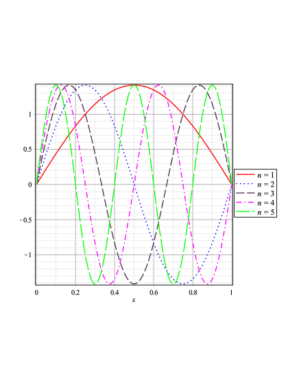
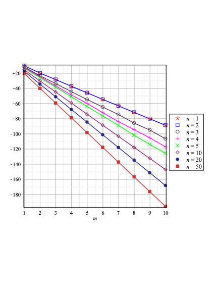
Figure 2: Graphs of approximations $\mathop{u_{n}}\limits^{10}(x)$ to first five eigenfunctions $u_{n}(x)$ with $n=1,2,3,4,5$ calculated according to the FD-method of rank $m=10$ for Example 2. Vertical axis $\mathop{u_{n}}\limits^{10}(x)$, horizontal axis $x$.

Figure 3: Graphs for broken lines joining the data points $\left(m;\ln\left(\delta_{n}(m)\right)\right)$ for Example 2. These graphs illustrates the behaviour of the norms of the corresponding residuals $\delta_{n}(m)$ (see notation (66)), i.e., they illustrate the exponential convergence of the FD-method with respect to the rank of FD-method $m$ for the eigenpairs $\mathop{u_{n}}\limits^{m}(x)$, $\mathop{\lambda_{n}}\limits^{m}$ with the indices $n=1,2,3,4,5,10,20,50$. Vertical axis $\ln\left(\delta_{n}(m)\right)$, horizontal axis $m$.

$m$	$\delta_{1}\left(m\right)$	$\delta_{2}\left(m\right)$	$\delta_{3}\left(m\right)$	$\delta_{4}\left(m\right)$	$\delta_{5}\left(m\right)$	$\delta_{10}\left(m\right)$	$\delta_{20}\left(m\right)$	$\delta_{50}\left(m\right)$
1	3.3e-5	1.7e-5	6.7e-6	2.7e-6	1.3e-6	1.5e-7	1.8e-8	1.1e-9
2	2.2e-9	2.1e-9	6.2e-11	2.0e-11	5.3e-12	6.5e-14	9.3e-16	3.7e-18
3	4.4e-13	2.7e-13	2.4e-15	8.5e-17	1.9e-17	3.0e-20	5.4e-23	1.4e-26
4	5.7e-17	5.5e-17	4.9e-20	7.0e-22	5.9e-23	1.4e-26	2.9e-30	4.6e-35
5	1.2e-20	6.7e-21	1.6e-24	8.8e-27	1.7e-28	6.4e-33	1.7e-37	1.7e-43
6	1.9e-24	1.8e-24	7.6e-29	4.7e-32	5.6e-34	2.9e-39	8.9e-45	5.8e-52
7	3.8e-28	2.3e-28	4.1e-33	3.5e-37	2.3e-39	1.3e-45	5.1e-52	2.1e-60
8	7.0e-32	6.8e-32	5.1e-38	9.2e-42	5.2e-45	6.0e-52	2.7e-59	7.1e-69
9	1.4e-35	8.6e-36	5.3e-42	1.9e-46	3.0e-50	2.8e-58	1.6e-66	2.6e-77
10	2.8e-39	2.7e-39	5.2e-47	1.2e-51	2.3e-55	1.3e-64	8.4e-74	8.8e-86

Table 4: Norms of the residuals $\delta_{n}(m)$ (see notation (66)) of FD-method of rank $m=1,2,...,10$ for the approximations to eigenpairs $\mathop{u_{n}}\limits^{m}(x)$, $\mathop{\lambda_{n}}\limits^{m}$ with the indices $n=1,2,3,4,5,10,20,50$ for Example 2.

 

Method	$n=1$	$n=2$	$n=3$	$n=4$	$n=5$	$n=10$	$n=20$	$n=50$
FDM	0.4e-2	2.5e-1	2.9	1.6+1	6.2e+1	4.0e+3	2.5e+5	5.9e+7
MNM	9.9e-7	2.9e-6	5.3e-5	5.3e-4	3.2e-3	8.1e-1	2.1e+2	3.6e+5
order6	5.2e-7	5.8e-7	1.1e-6	4.1e-7	4.7e-6	4.7e-3	4.9	4.8e+3
order8	8.9e-5	1.5e-3	7.4e-3	2.3e-2	5.7e-2	9.1e-1	1.4e+1	4.1e+3
order10	1.9e-5	3.0e-4	1.5e-3	4.7e-3	1.2e-2	1.8e-1	2.9	5.4e+2
FDM*	1.8e-6	1.2e-6	3.6e-6	2.0e-6	6.8e-7	1.7e-6	4.2e-6	1.2e-6
MNM*	9.1e-7	1.1e-5	4.4e-7	5.5e-6	4.5e-7	9.1e-7	6.7e-6	4.0e-6
order6*	3.0e-6	8.3e-6	3.9e-6	3.7e-6	2.1e-6	5.7e-6	7.6e-6	4.8e-6
order8*	7.9e-8	6.6e-7	1.5e-6	1.6e-7	2.0e-6	5.5e-7	3.7e-6	4.3e-7
order10*	3.1e-6	2.1e-6	2.5e-6	1.1e-6	2.4e-6	1.9e-6	2.9e-6	2.7e-7
ADM	1.2e-15	3.7e-13	2.0e-8	1.0e-2	2.8+2
SLEUTH	2.0e-8	2.8e-6	2.6e-6	5.9e-6	3.2e-6	3.4e-4	3.5e-2	5.4e-1

Table 5: Absolute differences in the approximations to eigenvalues from [21, Table 5] with respect to the numerical eigenvalues $\mathop{\lambda_{n}}\limits^{10}$, $n=1,2,3,4,5,10,20,50$ calculated according to the FD-method of rank $m=10$ for Example 2.

9 Conclusions

Results. In this article a new symbolic algorithmic implementation of the functional-discrete (FD-) method is developed and justified for the fourth order Sturm–Liouville problem (see numerical algorithm from Section 7). We consider the eigenvalue problem on a finite interval $[0,X]$ in the Hilbert space $L_{2}\left(0,X\right)$ for the fourth order ordinary differential equation (1) with polynomial coefficients (3) and boundary conditions (2). The sufficient conditions of an exponential convergence rate of FD-method are received (see Theorem 1). The obtained estimates of the absolute errors of FD-method (31), (32) significantly improve the accuracy of the estimates obtained earlier in [5]. The theoretical results are illustrated by numerical examples 1 and 2 in which the numerical results obtained with the FD-method are compared with the numerical test results obtained with other existing numerical techniques [16, 17, 18, 19, 20, 21].

Features of implementation. The obtained algorithm is symbolic and operates with the decomposition coefficients (19) of the eigenfunction corrections $u_{n}^{(j+1)}(x)$ in some basis on interval $\left[0,X\right]$ (see Lemma 2). Unlike the symbolic algorithm from [7] and traditional algorithm from [5, 10], presented approach produces explicit recursive formulas for the coefficients in (18) which are corresponding elements of the column vectors (55) and (56). These coefficients are represented recursively through the coefficients and quantities computed at previous steps of FD-method.

Unique advantages. Proposed symbolic algorithm of the simplest variant of the FD-method for problem (1)–(3) will always be convergent beginning with some eigenvalue index number $n_{0}$ (it can be large enough) with estimates of the absolute errors (31) and (32) (see Theorem 1). This means that by using the simplest variant of the FD-method one can obtain the asymptotic formulas for eigenvalues and eigenfunctions.

The approximate eigenpairs $\mathop{u_{n}}\limits^{m}(x)$, $\mathop{\lambda_{n}}\limits^{m}$ are computed exactly as analytical expressions and there are no rounding errors (see Remark 2). Proposed symbolic algorithm uses only the algebraic operations and basic operations on $(2\times 1)$ column vectors and $(2\times 2)$ matrices. Presented method does not require solving any boundary value problems and computations of any integrals, unlike the previous variants of FD-method from [5, 10]. Substituting into the obtained analytical expressions the given value $n$ and the numerical values of input data, we find numerical values of the corresponding approximations $\mathop{\lambda_{n}}\limits^{m}$, $\mathop{u_{n}}\limits^{m}(x)$.

FD-method converges exponentially with respect to rank $m$. Moreover the convergence of the FD-method increases together with the index $n$, unlike the accuracy degradation of other existing numerical techniques with the increasing of the eigenvalue index $n$.

Appendix A

Analytical formulas which are used for computation in the proposed numerical algorithm (see the step 4 and 11 of the numerical algorithm from Section 7):

$$\begin{split}&F_{n,\cos}^{(j+1)}(x)=\sum_{t=0}^{M(j)}x^{t}\sum_{s=\left.\left.\right]\kern-1.04996pt\right]\frac{t}{r+1}\left[\kern-1.04996pt\left[\right.\right.}^{j}\lambda_{n}^{(j+1-s)}b_{n,t}^{(s)}\\ &+\sum_{t=0}^{M(j+1)-1}x^{t}\sum_{l=\max(0,t-M(j))}^{\min(r,t)}\left(b_{n,t-l}^{(j)}\left(-A_{l}+C_{l}\left(\frac{\pi n}{X}\right)^{2}\right)-a_{n,t-l}^{(j)}B_{l}\frac{\pi n}{X}\right)\\ &-\sum_{t=0}^{M(j+1)-2}x^{t}\sum_{l=\max(0,t-M(j)+1)}^{\min(r,t)}\left(b_{n,t-l+1}^{(j)}B_{l}+a_{n,t-l+1}^{(j)}C_{l}2\frac{\pi n}{X}\right)\left(t-l+1\right)\\ &-\sum_{t=0}^{M(j+1)-3}x^{t}\sum_{l=\max(0,t-M(j)+2)}^{\min(r,t)}b_{n,t-l+2}^{(j)}C_{l}\left(t-l+2\right)\left(t-l+1\right),\end{split}$$

$$\begin{split}&F_{n,\sin}^{(j+1)}(x)=\sum_{t=0}^{M(j)}x^{t}\sum_{s=\left.\left.\right]\kern-1.04996pt\right]\frac{t}{r+1}\left[\kern-1.04996pt\left[\right.\right.}^{j}\lambda_{n}^{(j+1-s)}a_{n,t}^{(s)}\\ &+\sum_{t=0}^{M(j+1)-1}x^{t}\sum_{l=\max(0,t-M(j))}^{\min(r,t)}\left(n,a_{n,t-l}^{(j)}\left(-A_{l}+C_{l}\left(\frac{\pi n}{X}\right)^{2}\right)+b_{n,t-l}^{(j)}B_{l}\frac{\pi n}{X}\right)\\ &-\sum_{t=0}^{M(j+1)-2}x^{t}\sum_{l=\max(0,t-M(j)+1)}^{\min(r,t)}\left(a_{n,t-l+1}^{(j)}B_{l}-b_{n,t-l+1}^{(j)}C_{l}2\frac{\pi n}{X}\right)\left(t-l+1\right)\\ &-\sum_{t=0}^{M(j+1)-3}x^{t}\sum_{l=\max(0,t-M(j)+2)}^{\min(r,t)}a_{n,t-l+2}^{(j)}C_{l}\left(t-l+2\right)\left(t-l+1\right),\end{split}$$

$$\begin{split}&F_{n,\cosh}^{(j+1)}(x)=\sum_{t=0}^{M(j-1)}x^{t}\sum_{s\left.\left.=\right]\kern-1.04996pt\right]\frac{t}{r+1}\left[\kern-1.04996pt\left[+\right.\right.1}^{j}\lambda_{n}^{(j+1-s)}d_{n,t}^{(s)}\\ &-\sum_{t=0}^{M(j)-1}x^{t}\sum_{l=\max(0,t-M(j-1))}^{\min(r,t)}\left(d_{n,t-l}^{(j)}\left(A_{l}+C_{l}\left(\frac{\pi n}{X}\right)^{2}\right)+c_{n,t-l}^{(j)}B_{l}\frac{\pi n}{X}\right)\\ &-\sum_{t=0}^{M(j)-2}x^{t}\sum_{l=\max(0,t-M(j-1)+1)}^{\min(r,t)}\left(d_{n,t-l+1}^{(j)}B_{l}+c_{n,t-l+1}^{(j)}C_{l}2\frac{\pi n}{X}\right)\left(t-l+1\right)\\ &-\sum_{t=0}^{M(j)-3}x^{t}\sum_{l=\max(0,t-M(j-1)+2)}^{\min(r,t)}d_{n,t-l+2}^{(j)}C_{l}\left(t-l+2\right)\left(t-l+1\right),\end{split}$$

$$\begin{split}&F_{n,\sinh}^{(j+1)}(x)=\sum_{t=0}^{M(j-1)}x^{t}\sum_{s\left.\left.=\right]\kern-1.04996pt\right]\frac{t}{r+1}\left[\kern-1.04996pt\left[+\right.\right.1}^{j}\lambda_{n}^{(j+1-s)}c_{n,t}^{(s)}\\ &-\sum_{t=0}^{M(j)-1}x^{t}\sum_{l=\max(0,t-M(j-1))}^{\min(r,t)}\left(c_{n,t-l}^{(j)}\left(A_{l}+C_{l}\left(\frac{\pi n}{X}\right)^{2}\right)+d_{n,t-l}^{(j)}B_{l}\frac{\pi n}{X}\right)\\ &-\sum_{t=0}^{M(j)-2}x^{t}\sum_{l=\max(0,t-M(j-1)+1)}^{\min(r,t)}\left(c_{n,t-l+1}^{(j)}B_{l}+d_{n,t-l+1}^{(j)}C_{l}2\frac{\pi n}{X}\right)\left(t-l+1\right)\\ &-\sum_{t=0}^{M(j)-3}x^{t}\sum_{l=\max(0,t-M(j-1)+2)}^{\min(r,t)}c_{n,t-l+2}^{(j)}C_{l}\left(t-l+2\right)\left(t-l+1\right).\end{split}$$

These formulas enter into the expression (33). Here $\left.\left.\right]\kern-1.49994pt\right]y\left[\kern-1.49994pt\left[\right.\right.$ is the smallest integer greater than or equal to a real number $y$ (this is the function ceil(y) in Maple).

Appendix B

Analytical expressions for the integrals $\alpha_{n,t}$, $\beta_{n,t}$, $\eta_{n,t}$, $\mu_{n,t}$ which are used in (58) and exactly calculated in the case $t=0,1,...$ [25] (see step 2 in Section 7):

$$\begin{split}\alpha_{n,t}&=\int_{0}^{X}\xi^{t}\sin^{2}\left(\frac{\pi n}{X}\xi\right)d\xi=\frac{1}{2}\frac{X^{t+1}}{t+1}-\frac{1}{2}t!X^{t+1}\sum_{k=0}^{t-1}\frac{1}{(t-k)!(2\pi n)^{k+1}}\sin\left(\frac{\pi k}{2}\right),\end{split}$$

$$\begin{split}\beta_{n,t}=\frac{1}{2}\int_{0}^{X}\xi^{t}\sin\left(\frac{2\pi n}{X}\xi\right)d\xi=-t!X^{t+1}\frac{1}{2}\sum_{k=0}^{t-1}\frac{1}{(t-k)!(2\pi n)^{k+1}}\cos\left(\frac{\pi k}{2}\right),\end{split}$$

$$\begin{split}\eta_{n,t}&=\int_{0}^{X}\xi^{t}\sin\left(\frac{\pi n}{X}\xi\right)\cosh\left(\frac{\pi n}{X}\xi\right)d\xi=\frac{X^{t+1}t!}{\left(\sqrt{2}\pi n\right)^{t+1}}\cos\left(\frac{\pi t}{2}\right)\cos\left(\frac{\pi\left(t+1\right)}{4}\right)\\ \end{split}$$

$$\begin{split}&-\sum_{k=0}^{t}\frac{t!X^{t+1}\cos\left(\pi n\right)}{\left(t-k\right)!\left(\sqrt{2}\pi n\right)^{k+1}}\left[\cos\left(\frac{\pi\left(k+1\right)}{4}\right)\right.\cos\left(\frac{\pi k}{2}\right)\cosh\left(\pi n\right)\\ \end{split}$$

$$\begin{split}&-\left.\sin\left(\frac{\pi\left(k+1\right)}{4}\right)\sin\left(\frac{\pi k}{2}\right)\sinh\left(\pi n\right)\right],\end{split}$$

$$\begin{split}\mu_{n,t}&=\int_{0}^{X}\xi^{t}\sin\left(\frac{\pi n}{X}\xi\right)\sinh\left(\frac{\pi n}{X}\xi\right)d\xi=-\frac{X^{t+1}t!}{\left(\sqrt{2}\pi n\right)^{t+1}}\sin\left(\frac{\pi t}{2}\right)\sin\left(\frac{\pi\left(t+1\right)}{4}\right)\\ &+\sum_{k=0}^{t}\frac{t!X^{t+1}\cos\left(\pi n\right)}{\left(t-k\right)!\left(\sqrt{2}\pi n\right)^{k+1}}\left[\sin\left(\frac{\pi\left(k+1\right)}{4}\right)\sin\left(\frac{\pi k}{2}\right)\cosh\left(\pi n\right)\right.\\ &\left.-\cos\left(\frac{\pi\left(k+1\right)}{4}\right)\cos\left(\frac{\pi k}{2}\right)\sinh\left(\pi n\right)\right].\end{split}$$

Appendix C

The formula for the corrections of eigenvalues (see steps 3,10 in Section 7):

$$\begin{split}\lambda_{n}^{(j+1)}=&a_{n,0}^{(0)}\cdot\left(\sum_{t=0}^{M(j+1)-1}\right.\sum_{l=\max(0,t-M(j))}^{\min(r,t)}\left[\frac{\pi n}{X}B_{l}\left(\beta_{n,t}a_{n,t-l}^{(j)}-\alpha_{n,t}b_{n,t-l}^{(j)}\right)\right.\\ &-\left.\left(\beta_{n,t}b_{n,t-l}^{(j)}+\alpha_{n,t}a_{n,t-l}^{(j)}\right)\left(-A_{l}+\left(\frac{\pi n}{X}\right)^{2}C_{l}\right)\right]+\\ \sum_{t=0}^{M(j+1)-2}&\sum_{l=\max(0,t-M(j)+1)}^{\min(r,t)}\left(t-l+1\right)\left[B_{l}\left(\beta_{n,t}b_{n,t-l+1}^{(j)}+\alpha_{n,t}a_{n,t-l+1}^{(j)}\right)\right.\\ &\left.+2\frac{\pi n}{X}C_{l}\left(\beta_{n,t}a_{n,t-l+1}^{(j)}-\alpha_{n,t}b_{n,t-l+1}^{(j)}\right)\right]\\ +\sum_{t=0}^{M(j+1)-3}&\sum_{l=\max(0,t-M(j)+2)}^{\min(r,t)}\left(t-l+1\right)\left(t-l+2\right)C_{l}\left(\beta_{n,t}b_{n,t-l+2}^{(j)}+\alpha_{n,t}a_{n,t-l+2}^{(j)}\right)\\ +\sum_{t=0}^{M(j)-1}&\sum_{l=\max(0,t-M(j-1))}^{\min(r,t)}\left[\frac{\pi n}{X}B_{l}\left(\eta_{n,t}c_{n,t-l}^{(j)}+\mu_{n,t}d_{n,t-l}^{(j)}\right)\right.\\ &\left.+\left(\eta_{n,t}d_{n,t-l}^{(j)}+\mu_{n,t}c_{n,t-l}^{(j)}\right)\left(A_{l}+\left(\frac{\pi n}{X}\right)^{2}C_{l}\right)\right]\\ +\sum_{t=0}^{M(j)-2}&\sum_{l=\max(0,t-M(j-1)+1)}^{\min(r,t)}\left(t-l+1\right)\left[B_{l}\left(\eta_{n,t}d_{n,t-l+1}^{(j)}+\mu_{n,t}c_{n,t-l+1}^{(j)}\right)\right.\\ &\left.+2\frac{\pi n}{X}C_{l}\left(\eta_{n,t}c_{n,t-l+1}^{(j)}+\mu_{n,t}d_{n,t-l+1}^{(j)}\right)\right]\\ \end{split}$$

$$\begin{split}+\sum_{t=0}^{M(j)-3}&\left.\sum_{l=\max(0,t-M(j-1)+2)}^{\min(r,t)}\left(t-l+1\right)\left(t-l+2\right)C_{l}\left(\eta_{n,t}d_{n,t-l+2}^{(j)}+\mu_{n,t}c_{n,t-l+2}^{(j)}\right)\right).\end{split}$$

References

References

• [1] M. Armstrong, Basic Topology, Springer, New York, NY, 1983. doi:10.1007/978-1-4757-1793-8.
• [2] E. Allgower, K. Georg, Introduction to Numerical Continuation Methods, Society for Industrial and Applied Mathematics, Philadelphia, PA, USA, 2003.
URL https://dl.acm.org/citation.cfm?id=945750
• [3] V. Makarov, A functional-difference method of arbitrary order of accuracy for solving the Sturm-Liouville problem with piecewise-smooth coefficients, Dokl. Akad. Nauk SSSR 320 (1) (1991) 34–39.
• [4] V. Makarov, Y. Klymenko, Application of the FD-method to the solution of the Sturm-Liouville problem with coefficients of special form, Ukr. Math. J. 59 (8) (2007) 1264––1273. doi:10.1007/s11253-007-0086-0.
• [5] I. Gavrilyuk, V. Makarov, A. Popov, Super-exponentially convergent parallel algorithm for eigenvalue problems for the fourth order ODE’s, J. Numer. & Appl. Math. 100 (1) (2010) 60–81.
• [6] V. Makarov, N. Romanyuk, New properties of the FD-method in its applications to the Sturm-–Liouville problems, Dopov. Nats. Akad. Nauk Ukr. (2) (2014) 26––31. doi:10.15407/dopovidi2014.02.026.
• [7] V. Makarov, N. Romaniuk, New algorithmic implementation of the FD-method for a fourth–order Sturm–Liouville problem, in: International Conference of Young Mathematicians, Vol. Applied and Computational Mathematics, Institute of Mathematics of NAS of Ukraine, Kyiv, Ukraine, 2015, p. 106. doi:10.13140/RG.2.1.3320.1521.
• [8] V. Makarov, N. Romaniuk, Symbolic Algorithm of the Functional-Discrete Method for a Sturm–-Liouville Problem with a Polynomial Potential, Computational Methods in Applied Mathematicsdoi:10.1515/cmam-2017-0040.
• [9] I. Gavrilyuk, V. Makarov, N. Romaniuk, Super-Exponentially Convergent Parallel Algorithm for a Fractional Eigenvalue Problem of Jacobi–Type, Computational Methods in Applied Mathematics 18 (1) (2017) 21–32. doi:10.1515/cmam-2017-0010.
• [10] I. Gavrilyuk, V. Makarov, N. Romaniuk, Superexponentially convergent algorithm for an abstract eigenvalue problem with applications to ordinary differential equations, J. Math. Sci. 220 (3) (2017) 273–300. doi:10.1007/s10958-016-3184-4.
• [11] G. Adomian, Solving Frontier Problems of Physics: The Decomposition Method, Kluwer Academic Publishers, Springer Science+Business Media, Dordrecht, 1994. doi:10.1007/978-94-015-8289-6.
• [12] R. Rach, A bibliography of the theory and applications of the Adomian decomposition method, 1961–2011, Kybernetes 41 (7/8). doi:10.1108/k.2012.06741gaa.007.
• [13] J. Pryce, Numerical Solution of Sturm-–Liouville Problems, Clarendon Press, Oxford, New York, 1993.
URL https://trove.nla.gov.au/version/12826803
• [14] Z. Zhang, How many numerical eigenvalues can we trust?, Journal of Scientific Computing 65 (2) (2015) 455–466. doi:10.1007/s10915-014-9971-5.
• [15] L. N. Trefethen, Computing Numerically with Functions Instead of Numbers, Commun. ACM 58 (10) (2015) 91–97. doi:10.1145/2814847.
• [16] B. Attili, D. Lesnic, An efficient method for computing eigenelements of Sturm–Liouville fourth–order boundary value problems, Applied Mathematics and Computation 182 (2) (2006) 1247–1254. doi:10.1016/j.amc.2006.05.011.
• [17] M. Syam, H. Siyyam, An efficient technique for finding the eigenvalues of fourth–order Sturm–-Liouville problems, Chaos, Solitons & Fractals 39 (2) (2009) 659––665. doi:10.1016/j.chaos.2007.01.105.
• [18] M. Atay, S. Kartal, Computation of Eigenvalues of Sturm-Liouville Problems using Homotopy Perturbation Method, International Journal of Nonlinear Sciences and Numerical Simulation 11 (2) (2010) 1565–1339. doi:10.1515/IJNSNS.2010.11.2.105.
• [19] S. Abbasbandy, A. Shirzadi, A new application of the homotopy analysis method: Solving the Sturm–Liouville problems, Communications in Nonlinear Science and Numerical Simulation 16 (1) (2011) 112–126. doi:https://doi.org/10.1016/j.cnsns.2010.04.004.
• [20] B. Chanane, Accurate solutions of fourth order Sturm–-Liouville problems, Journal of Computational and Applied Mathematics 234 (10) (2010) 3064––3071. doi:10.1016/j.cam.2010.04.023.
• [21] A. Rattana, C. Böckmann, Matrix methods for computing eigenvalues of Sturm–-Liouville problems of order four, Journal of Computational and Applied Mathematics 249 (2013) 144 – 156. doi:10.1016/j.cam.2013.02.024.
• [22] N. Vilenkin, Combinatorics, Academic Press, Inc., 1971.
• [23] E. Reingold, J. Nievergelt, N. Deo, Combinatorial Algorithms: Theory and Practice, Prentice Hall College Div, 1977.
URL https://dl.acm.org/citation.cfm?id=1096489
• [24] G. Fichtenholz, Foundations of Mathematical Analysis, Vol. 1, Nauka, Moscow, 1968.
• [25] I. Gradshteyn, I. Ryzhik, Table of Integrals, Series, and Products, 8th Edition, Elsevier/Academic Press, Amsterdam, 2014.
• [26] D. Lozier, R. Boisvert, C. Clark (Eds.), NIST Handbook of Mathematical Functions, Cambridge University Press, 2010.
URL http://dlmf.nist.gov/13
• [27] L.Greenberg, M. Marletta, Algorithm 775: The Code SLEUTH for Solving Fourth–Order Sturm–Liouville Problems, ACM Transactions on Mathematical Software 23 (4) (1997) 453––493. doi:10.1145/279232.279231.