Multivector variate distributions: An application in Finance

Abstract

A new family of multivariate distributions, which shall be termed multivector variate distributions, based in the family of the multivariate contoured elliptically distribution is proposed. Several particular cases of multivector variate distributions are obtained and a number of published multivariate distributions in another contexts are found as simple corollaries. An application of interest in finance is full derived and compared with the traditional methods.

1 Introduction

Models of phenomena in nature are intrinsically complex and involve a priori several random variables which depend each other. The researcher expect to discover or model such laws in a parametric or non parametric way. With observational data the expert tries to estimates the model in order to fit or predict different stages of interest, however the mathematics behind a model allowing the stochastic dependency of the variables becomes complex very fast. Then some ideal assumptions must be made involving independent variables. To clarify this point, we consider a simple example. Consider to model probabilistically the precipitation and the streamflow, based on the knowledge of a probabilistic distribution for each variate. The last fact is usually simple to determine, because the expert can explain very well the marginal distributions of the models, however, the joint distribution of those two variables is difficult to handle. Then the behavior of both variables in a random bivariate is leaved to the artificial explanation under independency. In our example, it is clear that any occurrence of any event for streamflow depends on the occurrence of precipitation.

The literature has tackle the problem by constructing a dependent joint distribution via some transformation, but it is based on independent variables, see for example Nadarajah (2007) and Nadarajah (2013). That approach based in the knowledge of the marginal distributions is very interesting for application; in fact the above mention example in hydrology and similar ones in finance have motivated mathematical developments in such area, see also Chen and Novick (1984) and Olkin and Liu (2003), unfortunately, all of them are based in some way in independent variables.

From the theoretical point of view, the referred multivariate case has been generalizsed to the matrix case, by the so called bimatrix variate distributions, see Bekker et al. (2011) and Díaz-García, and Gutiérrez-Jáimez (2010a, b, 2011). The reader is also referred to Ehlers (2011), which provides a complete revision of the works about such complex problem.

We quote again that the best advantage of the model consists of knowing the marginal distribution of each variable, a simple requirement to fulfill in applied sciences, given the records of univariate random research. The main problem to solve consists of proposing a probabilistic dependent model with such marginal distributions. We set the solution as follows: Section 2 gives some results on Jacobians, integrals and elliptical distributions. Then Section 3 derives the family of joint distributions of several probabilistic dependent random vectors with known marginal distributions. Such distribution which is indexed by the general family of elliptical contoured distributions will be termed ”multi-vector variate distribution”. As corollaries, several particular distributions of the literature are derived straightforwardly, and a number of new distributions and versatile mixtures of distributions are provided in Section 4. In Section 5, distributions studied in previous section are extended to more general values of their parameters. Finally an applications in finance is full detailed in Section 6.

2 Preliminary results

In this section we shown some results about Jacobians, integration and multivariate elliptical contoured distributions necessary for the presentation of the results of this work. A detailed study of these and other results can be consulted in Fang and Zhang (1990), Fang et al. (1990) and Muirhead (2005).

First we propose some notations: if $\mathbf{A}\in\Re^{n\times m}$ denotes a matrix, this is, $\mathbf{A}$ have $n$ rows and $m$ columns, then $\mathbf{A}^{\prime}\in\Re^{m\times n}$ denotes its transpose matrix, and if $\mathbf{A}\in\Re^{n\times n}$ has an inverse, it shall be denoted by $\mathbf{A}^{-1}\in\Re^{n\times n}$. An identity matrix shall be denoted by $\mathbf{I}\in\Re^{n\times n}$, to specified the size of the identity, we will use $\mathbf{I}_{n}$. A null matrix shall be denoted as $\mathbf{0}\equiv\mathbf{0}_{n\times m}\in\Re^{n\times m}$. $\mathbf{A}\in\Re^{n\times n}$ is a symmetric matrix if $\mathbf{A}=\mathbf{A}^{\prime}$ and if all their eigenvalues are positive then $\mathbf{A}$ is positive definite matrix, which shall be denoted as $\mathbf{A}>\mathbf{0}$. The vectors shall be denoted also in bold style but in lower case. The Euclidean norm of a vector $\mathbf{x}=(x_{1},\ldots,x_{n})^{\prime}\in\Re^{n}$ will be denoted as $||\mathbf{x}||$ and is given by $\sqrt{\mathbf{x}^{\prime}\mathbf{x}}=\sqrt{\sum_{i=1}^{n}x_{i}^{2}}$.

From Muirhead (2005, Theorem 2.1.3, p.55), we have,

Theorem 2.1.

For the following transformation from rectangular coordinates $\mathbf{x}^{\prime}=(x_{1},\dots,x_{n})$ to polar coordinates $(s,\mathbf{h})^{\prime}=(s,\theta_{1},\dots,\theta_{n-1})$:

$$x_{1} = s\sin\theta_{1}\sin\theta_{2}\cdots\sin\theta_{n-2}\sin\theta_{n-1}$$

$$x_{2} = s\sin\theta_{1}\sin\theta_{2}\cdots\sin\theta_{n-2}\cos\theta_{n-1}$$

$$x_{3} = s\sin\theta_{1}\sin\theta_{2}\cdots\sin\theta_{n-3}\cos\theta_{n-2}$$

$$\vdots = \vdots$$

$$x_{n-1} = s\sin\theta_{1}\cos\theta_{2}$$

$$x_{n} = s\cos\theta_{1},$$

where, $s>0$, $\theta_{i}\in(0,\pi]$, $i=1,\dots,n-2$ and $\theta_{n-1}\in(0,2\pi]$. We have

$$\bigwedge_{i=1}^{n}dx_{i}=s^{n-1}\prod_{i=1}^{n-2}\sin^{n-i-1}\theta_{i}\left(\bigwedge_{i=}^{n-1}d\theta_{i}\right)\wedge ds.$$

In this results is defined $s^{2}=\|\mathbf{x}\|^{2}$. Then if we define $s=r^{2}$, we obtain

$$\bigwedge_{i=1}^{n}dx_{i}=2^{-1}r^{n/2-1}\prod_{i=1}^{n-2}\sin^{n-i-1}\theta_{i}\left(\bigwedge_{i=}^{n-1}d\theta_{i}\right)\wedge dr.$$

Denoting

$$\prod_{i=1}^{n-2}\sin^{n-i-1}\theta_{i}\left(\bigwedge_{i=}^{n-1}d\theta_{i}\right),$$

as $(\mathbf{h}^{\prime}d\mathbf{h})$, we obtain that

$$\bigwedge_{i=1}^{n}dx_{i}=2^{-1}r^{n/2-1}(\mathbf{h}^{\prime}d\mathbf{h})\wedge dr.$$

Moreover, from the proof of Muirhead (2005, Theorem 1.5.5, pp. 36-37 and Thoerem 2.1.15, p. 70), we have

$$\int_{\mathbf{h}\in\mathcal{V}_{1,n}}(\mathbf{h}^{\prime}d\mathbf{h})=\frac{2\pi^{n/2}}{\Gamma[n/2]},$$

where in general, $\mathcal{V}_{m,n}$ denotes the Stiefel manifold, the space of all matrices $\mathbf{H}_{1}\in\Re^{n\times m}$ ($n\geq m$) with orthogonal columns, so that $\mathbf{H}^{\prime}_{1}\mathbf{H}_{1}=\mathbf{I}_{m}$. Thus

$$\mathcal{V}_{m,n}=\{\mathbf{H}_{1}\in\Re^{n\times m}|\mathbf{H}^{\prime}_{1}\mathbf{H}_{1}=\mathbf{I}_{m}\}.$$

Note that, when $m=1$, then

$$\mathcal{V}_{1,n}=\{\mathbf{h}\in\Re^{n}:\|\mathbf{h}\|^{2}=1\},$$

the unit sphere in $\Re^{n}$. This is, of course, an $(n-1)$-dimensional surface in $\Re^{n}$, see Muirhead (2005, Section 2.1.4, pp. 67-72).

Thus we can propose an important Jacobian.

Theorem 2.2.

Let $\mathbf{y}=\left(1-||\mathbf{x}||^{2}\right)^{-\frac{1}{2}}\mathbf{x}$, with $\mathbf{x},\mathbf{y}\in\Re^{n}$, then

$$(d\mathbf{y})=\left(1-||\mathbf{x}||^{2}\right)^{-\left(\frac{n}{2}+1\right)}(d\mathbf{x}).$$

Proof.

Define $v=||\mathbf{y}||^{2}=\left(1-||\mathbf{x}||^{2}\right)^{-1}||\mathbf{x}||^{2}$ and $w=||\mathbf{x}||^{2}$, then by Muirhead (2005, Th. 2.1.14),

$$(d\mathbf{y})=2^{-1}v^{\frac{n}{2}-1}(dv)\wedge(\mathbf{h}^{\prime}d\mathbf{h}),\quad\mathbf{h}\in\mathcal{V}_{1,n}$$

and

$$(d\mathbf{x})=2^{-1}w^{\frac{n}{2}-1}(dw)\wedge(\mathbf{g}^{\prime}d\mathbf{g}),\quad\mathbf{g}\in\mathcal{V}_{1,n},$$

then

$$(dv)=2v^{-\left(\frac{n}{2}-1\right)}(d\mathbf{y})\wedge(\mathbf{h}^{\prime}d\mathbf{h}),\quad\mathbf{h}\in\mathcal{V}_{1,n}$$ (1)

and

$$(dw)=2w^{-\left(\frac{n}{2}-1\right)}(d\mathbf{x})\wedge(\mathbf{g}^{\prime}d\mathbf{g}),\quad\mathbf{g}\in\mathcal{V}_{1,n},$$ (2)

also $v=(1-w)^{-1}w=(1-w)^{-1}(1-(1-w))=(1-w)^{-1}-1$, thus

$$(dv)=\mbox{abs}\left(\frac{(dw)}{(1-w)^{2}}\right).$$ (3)

Uniqueness of $(\mathbf{h}^{\prime}d\mathbf{h})$ and substitution of (1) and (2) in (3) imply that $(d\mathbf{y})=\frac{v^{\frac{n}{2}-1}}{(1-w)^{2}}(d\mathbf{x})$. Thus using $\mathbf{y}=\left(1-||\mathbf{x}||^{2}\right)^{-\frac{1}{2}}\mathbf{x}$, $v=||\mathbf{y}||^{2}$ and $w=||\mathbf{x}||^{2}$, the required result is obtained. ∎

Next we provide from Muirhead (2005) a summary about elliptically contoured distribution theory; see also Fang and Zhang (1990) and Fang et al. (1990). Let $\mathbf{y}=(y_{1},\ldots,y_{n})^{\prime}\in\Re^{n}$, then $\mathbf{y}$ is said to have a multivariate elliptically contoured distribution if its characteristic function takes the form

$$\phi_{\mathbf{y}}(\mathbf{t})=\exp(i\mathbf{t}^{\prime}\boldsymbol{\mu})\psi(\mathbf{t}^{\prime}\boldsymbol{\Sigma}\mathbf{t}),$$

where $\mathbf{t}$ and $\boldsymbol{\mu}$ are n-dimensional vectors and $\psi:[0,\infty)\rightarrow\Re$, $|\psi(t)|\leq 1$ for $t\in\Re_{0}^{+}$. It implies that all marginal distributions are elliptical and all marginal density functions of dimension $k<n$ have the same functional form. For example, take $\mathbf{t}=(\mathbf{t}_{1}^{\prime}|\mathbf{0}^{\prime})^{\prime}$, $\mathbf{y}=\left(\begin{array}[]{c}\mathbf{y}_{1}\\ \mathbf{y}_{2}\\ \end{array}\right)$, $\boldsymbol{\mu}=\left(\begin{array}[]{c}\boldsymbol{\mu}_{1}\\ \boldsymbol{\mu}_{2}\\ \end{array}\right)$, $\boldsymbol{\Sigma}=\left(\begin{array}[]{cc}\boldsymbol{\Sigma}_{11}&\boldsymbol{\Sigma}_{12}\\ \boldsymbol{\Sigma}_{21}&\boldsymbol{\Sigma}_{22}\\ \end{array}\right)$, where $\mathbf{t}_{1}$, $\mathbf{y}_{1}$ and $\boldsymbol{\mu}_{1}$ are $k\times 1$ and $\boldsymbol{\Sigma}_{11}$ is $k\times k$, then via the characteristic function we have that $\mathbf{y}_{1}\sim\mathcal{E}_{k}(\boldsymbol{\mu}_{1},\boldsymbol{\Sigma}_{11},\psi)$. Provided they exist, $E(\mathbf{y})=\boldsymbol{\mu}$ and $\mathop{\rm Cov}\nolimits(\mathbf{y})=c\boldsymbol{\Sigma}$, where $c=-2\psi^{\prime}(0)$. Thus, all distributions in the class $\mathcal{E}_{n}(\boldsymbol{\mu},\boldsymbol{\Sigma},\psi)$ have the same mean $\boldsymbol{\mu}$ and the same correlation matrix $\mathbf{P}=(\rho_{ij})$, with

$$\rho_{ij}=\frac{\mathop{\rm Cov}\nolimits(y_{i},y_{j})}{\sqrt{\mathop{\rm Var}\nolimits(y_{i})}\sqrt{\mathop{\rm Var}\nolimits(y_{j})}}=\frac{c\sigma_{ij}}{\sqrt{c\sigma_{ii}}\sqrt{c\sigma_{jj}}}=\frac{\sigma_{ij}}{\sqrt{\sigma_{ii}}\sqrt{\sigma_{jj}}}.$$

Note that if any marginal distribution is normal, then $\mathbf{y}$ is normal. Observe also that if $\mathbf{y}=(y_{1},\ldots,y_{n})^{\prime}\sim\mathcal{N}_{n}(\boldsymbol{\mu},\boldsymbol{\Sigma})$, and $\boldsymbol{\Sigma}$ is diagonal, then $y_{1},\ldots,y_{n}$ are all independent. In general, let $\mathbf{y}=(y_{1},\ldots,y_{n})^{\prime}\sim\mathcal{E}_{n}(\boldsymbol{\mu},\boldsymbol{\Sigma},\psi)$ and $\boldsymbol{\Sigma}$ is diagonal, if $y_{1},\ldots,y_{n}$ are all independent, then $\mathbf{y}$ is normal.

Now, the density function of the elliptical contoured n-dimensional vector $\mathbf{y}$, with respect to the Lebesgue measure in $\Re^{n}$, is given by

$$dF_{\mathbf{y}}(\mathbf{y})=\frac{1}{|\boldsymbol{\Sigma}|^{1/2}}h\left\{\left[(\mathbf{y}-\boldsymbol{\mu})^{\prime}\boldsymbol{\Sigma}^{-1}(\mathbf{y}-\boldsymbol{\mu})\right]\right\}(d\mathbf{y}),$$ (4)

where $\boldsymbol{\mu}\in\Re^{n}$, $\boldsymbol{\Sigma}\in\Re^{n\times n}$, $\boldsymbol{\Sigma}>\mathbf{0}$ and $(d\mathbf{Y})=\bigwedge_{i=1}^{n}dy_{i},i=1,\ldots,n$. The function $h:\Re\rightarrow[0,\infty)$ is termed the generator function and satisfies $\int_{0}^{\infty}u^{n-1}h(u^{2})du<\infty$. Such a distribution is denoted by $\mathbf{y}\sim\mathcal{E}_{n}(\boldsymbol{\mu},\boldsymbol{\Sigma},h)$.

This class of distributions includes the Normal, t-Student (which includes the t and Cauchy distributions), Laplace, Bessel and Kotz, among other distributions. Some specific matrix-variate Elliptical densities are presented in Table 1, also see Fang and Zhang (1990).

Table 1: Explicit forms of the densities of the elliptical distributions.

Elliptical law	Density
Pearson VII	$\displaystyle\frac{\Gamma[q]}{(r\pi)^{n/2}\Gamma[q-n/2]\varrho}\left(1+\displaystyle\frac{W}{r}\right)^{-q}$
	$r>0$ and $q>n/2$
Kotz type	$\displaystyle\frac{sr^{(2q+n-2)/2s}\ \Gamma[n/2]}{\pi^{n/2}\Gamma\left[(2q+n-2)/2s\right]\varrho}\ W^{q-1}\exp\left(-rW^{s}\right)$
	$r,s>0$ and $2q+n>2$
Bessel	$\displaystyle\frac{W^{1/2}}{2^{q+n-1}\ \pi^{n/2}\ r^{n+q}\ \Gamma[q+n/2]\ \varrho}\ K_{q}\left(\displaystyle\frac{W^{1/2}}{r}\right)$
	$r>0$ and $q>-n/2$
Pearson II	$\displaystyle\frac{\Gamma[q+1+n/2]}{\pi^{n/2}\ \Gamma[q+1]\ \varrho}(1-W)^{q}$
	$q\in\Re$ and $W\leq 1$

When $\boldsymbol{\mu}=\mathbf{0}_{n}$, $\boldsymbol{\Sigma}=\mathbf{I}_{n}$ , such distribution is termed vector variate spherical distribution and shall be denoted as $\mathbf{Y}\sim\mathcal{E}_{n}(\mathbf{0},\mathbf{I}_{n},h)$. In other words, $\mathbf{y}$ is said to have a spherical distribution if $\mathbf{y}$ and $\mathbf{H}\mathbf{y}$ have the same distribution for all $n\times n$ orthogonal matrices $\mathbf{H}$. Moreover, the spherical density depends on $\mathbf{y}$ only through the value of $\mathbf{y}^{\prime}\mathbf{y}$.

Now, assume that $\mathbf{x}\sim\mathcal{E}_{n}(\mathbf{0},\mathbf{I},h)$, i.e.

$$dF_{\mathbf{x}}(\mathbf{x})=h(||\mathbf{x}||^{2})(d\mathbf{x}).$$

Consider the change of rectangular coordinates into polar coordinates, $\mathbf{x}\rightarrow(s,\mathbf{g})$, then by Theorem 2.1

$$dF_{s,\mathbf{g}}(s,\mathbf{g})=2^{-1}s^{n/2-1}h(s)(ds)\wedge(\mathbf{g}^{\prime}d\mathbf{g}),\quad s>0,||\mathbf{g}||^{2}=1.$$

Integration over $\mathbf{g}\in\mathcal{V}_{1,n}$ gives

$$dF_{s}(s)=\frac{\pi^{n/2}}{\Gamma[n/2]}s^{n/2-1}h(s)(ds),s>0.$$

Set $r=s^{1/2}$, then $(ds)=2r(dr)$ and

$$dF_{r}(r)=\frac{2\pi^{n/2}}{\Gamma[n/2]}s^{n-1}h(r^{2})(dr).$$

Observe also that

$$1=\int_{\mathbf{x}\in\Re^{n}}h(||\mathbf{x}||^{2})(dx),$$

so by the change of variable $z=as$, with $(ds)=\frac{(dz)}{a}$, we have that

$$1=\int_{s>0}\frac{\pi^{n/2}}{\Gamma[n/2]}s^{n/2-1}h(s)(ds)=\frac{\pi^{n/2}}{\Gamma[n/2]}\int_{z>0}\left(\frac{z}{a}\right)^{n/2-1}h\left(\frac{z}{a}\right)\frac{(dz)}{a}.$$

Thus we get that

$$\int_{z>0}z^{n/2-1}h\left(\frac{z}{a}\right)(dz)=\frac{a^{n/2}\Gamma[n/2]}{\pi^{n/2}}.$$ (5)

3 Multivector variate theory

In this apart we derive a number of multivector variate distribution. The technique can be replicated with several mixtures or marginal distributions, which depends on the particular phenomena of interest and a previous knowledge of the marginal distributions.

3.1 Multivector variate elliptical distribution

Assume that $\mathbf{x}\sim\mathcal{E}_{n}(\boldsymbol{\mu},\boldsymbol{\Sigma},h)$, with $\boldsymbol{\Sigma}>\mathbf{0}$, then

$$dF_{\mathbf{x}}(\mathbf{x})=|\boldsymbol{\Sigma}|^{-\frac{1}{2}}h\left((\mathbf{x}-\boldsymbol{\mu})^{\prime}\boldsymbol{\Sigma}^{\prime}(\mathbf{x}-\boldsymbol{\mu})\right)(d\mathbf{x}).$$

Now consider the following partition of $\mathbf{x}$, $\boldsymbol{\mu}$ and $\boldsymbol{\Sigma}$

$$\mathbf{x}=\left(\begin{array}[]{c}\mathbf{x}_{1}\\ \vdots\\ \mathbf{x}_{k}\end{array}\right)\in\Re^{n},\boldsymbol{\mu}=\left(\begin{array}[]{c}\boldsymbol{\mu_{1}}\\ \vdots\\ \boldsymbol{\mu_{k}}\end{array}\right),\mathbf{x}_{i},\boldsymbol{\mu}_{i}\in\Re^{n_{i}},\sum_{i=1}^{k}n_{i}=n,$$

$$\boldsymbol{\Sigma}=\left(\begin{array}[]{cccc}\boldsymbol{\Sigma}_{11}&\mathbf{0}&\cdots&\mathbf{0}\\ \mathbf{0}&\boldsymbol{\Sigma}_{22}&\cdots&\mathbf{0}\\ \vdots&\vdots&\ddots&\vdots\\ \mathbf{0}&\mathbf{0}&\cdots&\boldsymbol{\Sigma}_{kk}\\ \end{array}\right),\boldsymbol{\Sigma}_{ii}>\mathbf{0},\boldsymbol{\Sigma}_{ii}\in\Re^{n_{i}\times n_{i}},i=1,\ldots,k.$$

Then we have

$$dF_{\mathbf{x}_{1},\ldots,\mathbf{x}_{k}}(\mathbf{x}_{1},\ldots,\mathbf{x}_{k})=\prod_{i=1}^{k}|\boldsymbol{\Sigma}_{ii}|^{-1/2}h\left(\sum_{i=1}^{k}(\mathbf{x}_{i}-\boldsymbol{\mu}_{i})^{\prime}\boldsymbol{\Sigma}_{ii}^{-1}(\mathbf{x}_{i}-\boldsymbol{\mu}_{i})\right)\bigwedge_{i=1}^{k}(d\mathbf{x}_{i}).$$ (8)

This joint distribution define a multivector variate which shall be termed multivector variate elliptical distribution. It will be denoted as

$$\mathbf{x}=\left(\begin{array}[]{c}\mathbf{x}_{1}\\ \vdots\\ \mathbf{x}_{k}\end{array}\right)\sim\mathcal{ME}_{n}(n_{1},\ldots,n_{k};\boldsymbol{\mu_{1}},\ldots,\boldsymbol{\mu_{k}};\boldsymbol{\Sigma_{11}},\ldots,\boldsymbol{\Sigma_{kk}};h).$$

3.2 Multivector variate log-elliptical distribution

Now assume that $\mathbf{x}=\log\mathbf{v}$, $\mathbf{x},\mathbf{v}\in\Re^{n}$, and $\log\mathbf{v}=(\log v_{1},\ldots,\log v_{n})^{\prime}$. If $\mathbf{x}\sim\mathcal{E}_{n}(\boldsymbol{\mu},\boldsymbol{\Sigma},h)$, then $\mathbf{v}$ is said to have a log-elliptical distribution, see Fang et al. (1990).

Consider that $\mathbf{x}=\log\mathbf{v}\sim\mathcal{ME}_{n}(n_{1},\ldots,n_{k};\boldsymbol{\mu_{1}},\ldots,\boldsymbol{\mu_{k}};\boldsymbol{\Sigma_{11}},\ldots,\boldsymbol{\Sigma_{kk}};h)$, where $\mathbf{x}_{i}=\log\mathbf{v}_{i}$, $i=1,\ldots,k$, then we say that $\mathbf{v}=(\mathbf{v}_{1},\ldots,\mathbf{v}_{k})^{\prime}$ has a multivector log-elliptical distribution, denoted as

$$\mathbf{v}=\left(\begin{array}[]{c}\mathbf{v}_{1}\\ \vdots\\ \mathbf{v}_{k}\end{array}\right)\sim\mathcal{MLE}_{n}(n_{1},\ldots,n_{k};\boldsymbol{\mu_{1}},\ldots,\boldsymbol{\mu_{k}};\boldsymbol{\Sigma_{11}},\ldots,\boldsymbol{\Sigma_{kk}};h).$$

Moreover, making the change of variable $(\mathbf{x}_{1},\ldots,\mathbf{x}_{k})^{\prime}=(\log\mathbf{v}_{1},\ldots,\log\mathbf{v}_{k})^{\prime}$, we have that

$$\bigwedge_{i=1}^{k}(d\mathbf{x}_{i}) = \left(\prod_{i=1}^{n_{1}}v_{i}^{-1}\right)\cdots\left(\prod_{i=1}^{n_{k}}v_{i}^{-1}\right)\bigwedge_{i=1}^{k}(d\mathbf{v}_{i})$$

$$= \prod_{j=1}^{k}\prod_{i=1}^{n_{j}}v_{i}^{-1}\bigwedge_{i=1}^{k}(d\mathbf{v}_{i}).$$

And by (8) we obtain

$$dF_{\mathbf{v}_{1},\ldots,\mathbf{v}_{k}}(\mathbf{v}_{1},\ldots,\mathbf{v}_{k})=\prod_{j=1}^{k}\left[|\boldsymbol{\Sigma}_{jj}|^{-n/2}\left(\prod_{i=1}^{n_{j}}v_{i}^{-1}\right)\right]\hskip 170.71652pt$$

$$\hskip 113.81102pt\times h\left(\sum_{i=1}^{k}(\log\mathbf{v}_{i}-\boldsymbol{\mu}_{i})^{\prime}\boldsymbol{\Sigma}_{ii}^{-1}(\log\mathbf{v}_{i}-\boldsymbol{\mu}_{i})\right)\bigwedge_{i=1}^{k}(d\mathbf{v}_{i})$$ (9)

This distribution is multifunctional because we can find a number of new models. For example, we can obtain multivector variate mixed distribution, namely, a part of the multivector $\mathbf{v}$ can follow a multivector variate elliptical distribution and the remaining part indexed by multivector variate log-elliptical law. This fact will be denoted as

$$\left(\begin{array}[]{c}\mathbf{x}\\ \mathbf{v}\\ \end{array}\right)=\left(\begin{array}[]{c}\mathbf{x}_{1}\\ \vdots\\ \mathbf{x}_{k_{1}}\\ \mathbf{v}_{1}\\ \vdots\\ \mathbf{v}_{k_{2}}\end{array}\right)\sim\mathcal{MELE}_{n}(n_{1},\ldots,n_{k};\boldsymbol{\mu_{1}},\ldots,\boldsymbol{\mu_{k}};\boldsymbol{\Sigma_{11}},\ldots,\boldsymbol{\Sigma_{kk}};h),$$

with $k_{1}+k_{2}=k$, $\mathbf{x}_{i}\in\Re^{n_{i}}$, $\mathbf{v}_{i}\in\Re^{n_{i}}$, $n=\sum_{i=1}^{k}n_{i}$ and the corresponding joint distribution is given by

$$dF_{\mathbf{x}_{1},\ldots,\mathbf{x}_{k_{1}},\mathbf{v}_{1},\ldots,\mathbf{v}_{k_{2}}}(\mathbf{x}_{1},\ldots,\mathbf{x}_{k_{1}},\mathbf{v}_{1},\ldots,\mathbf{v}_{k_{2}})\hskip 170.71652pt$$

$$=\prod_{i=1}^{k_{1}}|\boldsymbol{\Sigma}_{ii}|^{-n/2}\prod_{j=1}^{k_{2}}\left[|\boldsymbol{\Sigma}_{jj}|^{-n/2}\left(\prod_{r=1}^{n_{j}}v_{r}^{-1}\right)\right]\hskip 56.9055pt$$

$$\times h\left(\sum_{i=1}^{k_{1}}(\mathbf{x}_{i}-\boldsymbol{\mu}_{i})^{\prime}\boldsymbol{\Sigma}_{ii}^{-1}(\log\mathbf{x}_{i}-\boldsymbol{\mu}_{i})\right.\hskip 28.45274pt$$

$$\hskip 71.13188pt+\left.\sum_{j=1}^{k_{2}}(\log\mathbf{v}_{j}-\boldsymbol{\mu}_{j})^{\prime}\boldsymbol{\Sigma}_{jj}^{-1}(\log\mathbf{v}_{j}-\boldsymbol{\mu}_{j})\right)\bigwedge_{i=1}^{k_{1}}(d\mathbf{x}_{i})\bigwedge_{j=1}^{k_{2}}(d\mathbf{v}_{j}).$$

Note that in this distribution, the variables $\mathbf{x}_{i}$, $i=1,\dots,k_{1}$ are probabilistically dependent, the same property follows for the variables $\mathbf{v}_{r}$, $r=1,\dots,k_{2}$. Moreover, for all $i=1,\dots,k_{1}$ and $r=1,\dots,k_{2}$, the variates $\mathbf{x}_{i}$ and $\mathbf{v}_{r}$ are also probabilistically dependent. This family of distribution can be termed as multivector variate elliptical-log-elliptical distribution. In particular, for $k_{1}=k_{2}=1$ this distribution can be proposed as the joint distribution for modeling two random variables $x$ and $v$ with certain marginal distribution; for example, $x$ could follow a $t$-Student distribution and $v$ a $\log$ $t$-Student distribution; we highlight again that the addressed joint distribution considers a probabilistic dependency between the two random variables $x$ and $v$.

3.3 Multivector variate T-distribution (or Pearson type VII)

Recall that if $\mathbf{x}\sim\mathcal{N}_{n}(\mathbf{0},\mathbf{I})$ and $s^{2}\sim\chi_{\nu}^{2}$ are independent, then $\mathbf{t}=s^{-1}\mathbf{x}$ has a multivariate t distribution. Now consider that

$$\left(\begin{array}[]{c}\mathbf{x}_{0}\\ \mathbf{x}_{1}\\ \vdots\\ \mathbf{x}_{k}\end{array}\right)\sim\mathcal{ME}_{n}(n_{0},\ldots,n_{k};\mathbf{0},\ldots,\mathbf{0};\sigma_{0}^{2}\mathbf{I}_{n_{0}},\ldots,\sigma_{k}^{2}\mathbf{I}_{n_{k}};h),$$

and define $s_{0}=||\mathbf{x}_{0}||^{2}$ and $\mathbf{t}_{i}=s_{0}^{-1/2}\mathbf{x}_{i}$, $i=1,\ldots,k$. Then

$$\bigwedge_{i=0}^{k}(d\mathbf{x}_{i})=2^{-1}s_{0}^{n_{0}/2-1}\prod_{i=1}^{k}s_{0}^{n_{i}/2}(ds_{0})\wedge(\mathbf{g}^{\prime}d\mathbf{g})\wedge\left(\bigwedge_{i=1}^{k}(d\mathbf{t}_{i})\right),\quad\mathbf{g}\in\mathcal{V}_{1,n_{0}}.$$

Thus

$$dF_{\mathbf{x}_{0},\ldots,\mathbf{x}_{k}}(\mathbf{x}_{0},\ldots,\mathbf{x}_{k})=\left(\prod_{i=1}^{k}\sigma_{i}^{-n_{i}}\right)h\left(\sum_{i=0}^{k}\sigma_{i}^{-2}||\mathbf{x}_{i}||^{2}\right)\bigwedge_{i=1}^{k}(d\mathbf{x}_{i})$$ (10)

so

$$dF_{s_{0},\mathbf{g},\mathbf{t}_{1},\ldots,\mathbf{t}_{k}}(s_{0},\mathbf{g},\mathbf{t}_{1},\ldots,\mathbf{t}_{k})=\frac{s_{0}^{n^{*}/2-1}}{2\prod_{i=0}^{k}\sigma_{i}^{n_{i}}}\hskip 170.71652pt$$

$$\hskip 56.9055pt\times h\left(\sigma_{0}^{-2}s_{0}+s_{0}\sum_{i=1}^{k}\sigma_{i}^{-2}||\mathbf{t}_{i}||^{2}\right)(ds_{0})\wedge(\mathbf{g}^{\prime}d\mathbf{g})\wedge\bigwedge_{i=1}^{k}(d\mathbf{t}_{i}),$$ (11)

where $n^{*}=n_{0}+n_{1}+\cdots+n_{k}$. Integration over $\mathbf{g}\in\mathcal{V}_{1,n_{0}}$ gives

$$dF_{s_{0},\mathbf{t}_{1},\ldots,\mathbf{t}_{k}}(s_{0},\mathbf{t}_{1},\ldots,\mathbf{t}_{k})=\frac{\pi^{n_{0}/2}}{\Gamma\left[n_{0}/2\right]\prod_{i=0}^{k}\sigma_{i}^{n_{i}}}s_{0}^{n^{*}/2-1}\hskip 113.81102pt$$

$$\hskip 56.9055pt\times h\left(\sigma_{0}^{-2}\left(1+\sigma_{0}^{2}\sum_{i=1}^{k}\sigma_{i}^{-2}||\mathbf{t}_{i}||^{2}\right)s_{0}\right)(ds_{0})\wedge\left(\bigwedge_{i=1}^{k}(d\mathbf{t}_{i})\right).$$ (12)

Remark 3.1.

According to the definition of this distribution, we shall see that the random variable $s_{0}$ follows a generalised $\chi^{2}$ distribution (or generalised gamma distribution), see Fang and Zhang (1990), and $\mathbf{t}=(\mathbf{t}^{\prime}_{1},\dots,\mathbf{t}^{\prime}_{k})^{\prime}$ has a multivector variate $t$-distribution (or Pearson type VII). Also note that $s_{0}$ and $\mathbf{t}$ are probabilistically dependent. Finally, this family of distribution defines a multivector variate $\chi^{2}$ generalisada-$t$ distribution.

From (5), the integral with respect to $s_{0}$ is given by

$$dF_{\mathbf{t}_{1},\ldots,\mathbf{t}_{k}}(\mathbf{t}_{1},\ldots,\mathbf{t}_{k})=\frac{\Gamma\left[n^{*}/2\right]\sigma_{0}^{n^{*}/2}}{\Gamma\left[n_{0}/2\right]\pi^{n^{*}/2}\prod_{i=0}^{k}\sigma_{i}^{n_{i}}}\hskip 170.71652pt$$

$$\hskip 142.26378pt\times\left(1+\sigma_{0}^{2}\sum_{i=1}^{k}\sigma_{i}^{-2}||\mathbf{t}_{i}||^{2}\right)^{-n^{*}/2}\bigwedge_{i=1}^{k}(d\mathbf{t}_{i}).$$ (13)

Finally, let $\beta_{i}=\sigma_{i}^{2}/\sigma_{0}^{2}$, then

$$dF_{\mathbf{t}_{1},\ldots,\mathbf{t}_{k}}(\mathbf{t}_{1},\ldots,\mathbf{t}_{k})=\frac{\Gamma\left[n^{*}/2\right]\prod_{i=1}^{k}\beta_{i}^{-n_{i}/2}}{\Gamma\left[n_{0}/2\right]\pi^{n^{*}/2}}\hskip 170.71652pt$$

$$\hskip 142.26378pt\times\left(1+\sum_{i=1}^{k}\beta_{i}^{-1}||\mathbf{t}_{i}||^{2}\right)^{-n^{*}/2}\bigwedge_{i=1}^{k}(d\mathbf{t}_{i}).$$ (14)

We refer it as the multivector variate t distribution and it will be denoted by

$$\mathbf{t}=\left(\begin{array}[]{c}\mathbf{t}_{1}\\ \vdots\\ \mathbf{t}_{k}\end{array}\right)\sim\mathcal{M}t_{n}(n_{0},\ldots,n_{k};\beta_{1},\ldots,\beta_{k}).$$

3.4 Multivector variate Pearson type II

Recall that if $s^{2}\sim\chi_{\nu}^{2}$ and $\mathbf{x}\sim\mathcal{N}_{n}(\mathbf{0},\mathbf{I})$ are independent, then $\mathbf{r}=(s^{2}+||\mathbf{x}||^{2})^{-n/2}\mathbf{x}$ is said to have a multivariate Pearson type II distribution. Moreover, if $\mathbf{t}$ has a multivariate t distribution, then $\mathbf{r}=(1+||\mathbf{t}||^{2})^{-n/2}\mathbf{t}$ has also a Person type II distribution, see Dickey (1967).

With that remark in mind, assume that $\mathbf{t}\sim\mathcal{M}t_{n}(n_{0},\ldots,n_{k};\beta_{1},\ldots,\beta_{k})$ and define $\mathbf{t}_{i}=(1-||\mathbf{r}_{i}||^{2})^{-n/2}\mathbf{r}_{i}$, $i=1,\ldots,k$, then

$$\bigwedge_{i=1}^{k}(d\mathbf{t}_{i})=\prod_{i=1}^{k}(1-||\mathbf{r}_{i}||^{2})^{-\left(n_{i}/2+1\right)}\bigwedge_{i=1}^{k}(d\mathbf{r}_{i}).$$

And

$$dF_{\mathbf{r}_{1},\ldots,\mathbf{r}_{k}}(\mathbf{r}_{1},\ldots,\mathbf{r}_{k})=\frac{\Gamma\left[n^{*}/2\right]\prod_{i=1}^{k}\beta_{i}^{-n_{i}/2}}{\Gamma\left[n_{0}/2\right]\pi^{n^{*}/2}}\hskip 170.71652pt$$

$$\times\left(1+\sum_{i=1}^{k}\beta_{i}^{-1}||(1-||\mathbf{r}_{i}||^{2})^{-n/2}\mathbf{r}_{i}||^{2}\right)^{-n^{*}/2}\prod_{i=1}^{k}(1-||\mathbf{r}_{i}||^{2})^{-\left(n_{i}/2+1\right)}\bigwedge_{i=1}^{k}(d\mathbf{r}_{i}).$$

Noting that

$$1+\sum_{i=1}^{k}\beta_{i}^{-1}||(1-||\mathbf{r}_{i}||^{2})^{-n/2}\mathbf{r}_{i}||^{2}=\prod_{i=1}^{k}\left(1-||\mathbf{r}_{i}||^{2}\right)^{-1}\hskip 142.26378pt$$

$$\hskip 85.35826pt\times\left(\prod_{i=1}^{k}\left(1-||\mathbf{r}_{i}||^{2}\right)+\sum_{i=1}^{k}\prod_{j=1,j\neq i}^{k}\beta_{i}^{-1}\left(1-||\mathbf{r}_{j}||^{2}\right)||\mathbf{r}_{i}||^{2}\right).$$

Then

$$dF_{\mathbf{r}_{1},\ldots,\mathbf{r}_{k}}(\mathbf{r}_{1},\ldots,\mathbf{r}_{k})=\frac{\Gamma\left[n^{*}/2\right)\prod_{i=1}^{k}\beta_{i}^{-n_{i}/2}}{\Gamma\left[n_{0}/2\right]\pi^{n^{*}/2}}\prod_{i=1}^{k}(1-||\mathbf{r}_{i}||^{2})^{\sum_{j=1,j\neq i}^{k}\left(n_{i}/2+1\right)-1}$$

$$\times\left(\prod_{i=1}^{k}\left(1-||\mathbf{r}_{i}||^{2}\right)+\sum_{i=1}^{k}\prod_{j=1,j\neq i}^{k}\beta_{i}^{-1}\left(1-||\mathbf{r}_{j}||^{2}\right)||\mathbf{r}_{i}||^{2}\right)^{-n^{*}/2}\bigwedge_{i=1}^{k}(d\mathbf{r}_{i}).$$

This law shall be termed multivector variate Pearson type II distribution, with notation

$$\mathbf{r}=\left(\begin{array}[]{c}\mathbf{r}_{1}\\ \vdots\\ \mathbf{r}_{k}\end{array}\right)\sim\mathcal{MP}^{II}_{n}(n_{0},\ldots,n_{k};\beta_{1},\ldots,\beta_{k}).$$

In a similar way to the multivector variate $\chi^{2}$ generalised t distribution, if we define $\mathbf{t}_{i}=(1-||\mathbf{r}_{i}||^{2})^{-n/2}\mathbf{r}_{i}$, $i=1,\ldots,k$, then we obtain the so called multivector variate $\chi^{2}$ generalised-Pearson type II distribution:

$$dF_{s_{0},\mathbf{r}_{1},\ldots,\mathbf{r}_{k}}(s_{0},\mathbf{r}_{1},\ldots,\mathbf{r}_{k})=\frac{\pi^{n_{0}/2}s_{0}^{n^{*}/2-1}}{\Gamma\left[n_{0}/2\right]\prod_{i=1}^{k}\sigma_{i}^{n_{i}}}\hskip 142.26378pt$$

$$\times h\left(\sigma_{0}^{-2}\left(1+\sigma_{0}^{2}\sum_{i=1}^{k}\sigma_{i}^{-2}||(1-||\mathbf{r}_{i}||^{2})^{-n/2}\mathbf{r}_{i}||^{2}\right)s_{0}\right)$$

$$\times\prod_{i=1}^{k}(1-||\mathbf{r}_{i}||^{2})^{-(n_{i}/2+1)}(ds_{0})\wedge\left(\bigwedge_{i=1}^{k}(d\mathbf{r}_{i})\right),\hskip 42.67912pt$$

$$=\frac{\pi^{n_{0}/2}s_{0}^{n^{*}/2-1}}{\Gamma\left[n_{0}/2\right]\prod_{i=1}^{k}\sigma_{i}^{n_{i}}}h\left(\sigma_{0}^{-2}\left(1+\sigma_{0}^{2}\sum_{i=1}^{k}\sigma_{i}^{-2}(1-||\mathbf{r}_{i}||^{2})||\mathbf{r}_{i}||^{2}\right)s_{0}\right)$$

$$\times\prod_{i=1}^{k}(1-||\mathbf{r}_{i}||^{2})^{-(n_{i}/2+1)}(ds_{0})\wedge\left(\bigwedge_{i=1}^{k}(d\mathbf{r}_{i})\right)\hskip 42.67912pt.$$

Note that the procedure implemented in this section can be generalised and used for deriving an uncountable number of combinations of families of distributions in the setting of multivector variate distributions.

4 Some related distributions

In this section we derive several consequences implicit in the results of the previous apart. In general, we start with a multivector variate distribution and we are interested in the joint distribution of the square norms of each subvector, the the multivariate distribution is obtained in such way that the random components are probabilistically dependent. In the same way a logarithmic distribution and its generalisation are derived. Moreover, several particular distributions of the literature are derived straightforwardly. We also remark that the distributions here derived are of a multivariate type.

4.1 Multivariate generalised $\chi^{2}$ distribution

Assume that

$$\mathbf{x}=(\mathbf{x}_{1}^{\prime},\ldots,\mathbf{x}_{k}^{\prime})^{\prime}\sim\mathcal{ME}_{n}(n_{1},\ldots,n_{k};\mathbf{0},\ldots,\mathbf{0};\sigma_{1}^{2}\mathbf{I}_{n_{1}},\ldots,\sigma_{k}^{2}\mathbf{I}_{n_{k}};h),$$

this is

$$\mathbf{x}=\left(\begin{array}[]{c}\mathbf{x}_{1}\\ \vdots\\ \mathbf{x}_{k}\end{array}\right)\in\Re^{n},\boldsymbol{\mu}=\left(\begin{array}[]{c}\mathbf{0}\\ \vdots\\ \mathbf{0}\end{array}\right),\mathbf{x}_{i}\in\Re^{n_{i}},\sum_{i=1}^{k}n_{i}=n,$$

$$\boldsymbol{\Sigma}=\left(\begin{array}[]{cccc}\sigma_{1}^{2}\mathbf{I}_{n_{1}}&\mathbf{0}&\cdots&\mathbf{0}\\ \mathbf{0}&\sigma_{2}^{2}\mathbf{I}_{n_{2}}&\cdots&\mathbf{0}\\ \vdots&\vdots&\ddots&\vdots\\ \mathbf{0}&\mathbf{0}&\cdots&\sigma_{k}^{2}\mathbf{I}_{n_{k}}\\ \end{array}\right),$$

where $\sigma_{i}^{2}>0$ for all $i=1,\ldots,k$.

Then

$$dF_{\mathbf{x}_{1},\ldots,\mathbf{x}_{k}}(\mathbf{x}_{1},\ldots,\mathbf{x}_{k})=\prod_{i=1}^{k}(\sigma_{i})^{n_{i}/2}h\left(\sum_{i=1}^{k}\sigma_{i}^{-2}||\mathbf{x}_{i}||^{2}\right)\bigwedge_{i=1}^{k}(d\mathbf{x}_{i}).$$

Define $u_{i}=||\mathbf{x}_{i}||^{2}$, then writing $\mathbf{x}_{i}=t_{i}\mathbf{g}_{i},$ $t_{i}>0$, $i=1,\ldots,k$, $\mathbf{g}_{i}\in\mathcal{V}_{1,n_{i}}$. We have that $u_{i}=||\mathbf{x}_{i}||^{2}=||t_{i}\mathbf{g}_{i}||^{2}=t_{i}^{2}||\mathbf{g}_{i}||^{2}=t_{i}^{2}$. Then

$$\bigwedge_{i=1}^{k}(d\mathbf{x}_{i})=\bigwedge_{i=1}^{k}\left(2^{-1}u_{i}^{n_{i}/2-1}(du_{i})(\mathbf{g}_{i}^{\prime}d\mathbf{g}_{i})\right)=2^{-k}\prod_{i=1}^{k}u_{i}^{n_{i}/2-1}\bigwedge_{i=1}^{k}(du_{i})\wedge\bigwedge_{i=1}^{k}(\mathbf{g}_{i}^{\prime}d\mathbf{g}_{i}).$$

Observing that

$$\int_{\mathbf{g}_{1}\in\mathcal{V}_{1,n_{1}}}\cdots\int_{\mathbf{g}_{k}\in\mathcal{V}_{1,n_{k}}}\bigwedge_{i=1}^{k}(\mathbf{g}_{i}^{\prime}d\mathbf{g}_{i}) = \prod_{i=1}^{k}\int_{\mathbf{g}_{i}\in\mathcal{V}_{1,n_{i}}}(\mathbf{g}_{i}^{\prime}d\mathbf{g}_{i})=\prod_{i=1}^{k}\frac{2\pi^{n_{i}/2}}{\Gamma\left[n_{i}/2\right]}$$ (17)

$$= \frac{2^{k}\pi^{n/2}}{\prod_{i=1}^{k}\Gamma\left[n_{i}/2\right]},$$

where $n=n_{1}+\cdots+n_{k}$. Then, we finally obtain

$$dF_{u_{1},\ldots,u_{k}}(u_{1},\ldots,u_{k})=\frac{\pi^{n/2}}{\prod_{i=1}^{k}\left(\sigma_{i}^{n_{i}}\Gamma\left[n_{i}/2\right]\right)}h\left(\sum_{i=1}^{k}\sigma_{i}^{-2}u_{i}\right)\prod_{i=1}^{k}u_{i}^{n_{i}/2-1}\bigwedge_{i=1}^{k}(du_{i}),$$ (18)

which shall be termed multivariate generalised $\chi^{2}$ distribution, a function denoted by

$$\mathbf{u}=\left(\begin{array}[]{c}u_{1}\\ \vdots\\ u_{k}\\ \end{array}\right)\sim\mathcal{G}\chi_{k}^{2}\left(n_{1},\ldots,n_{k};\sigma_{1}^{2},\ldots,\sigma_{k}^{2};h\right).$$

This sets a proposal for different multivariate distributions, with probabilistic dependent elements, see Chen and Novick (1984), Libby and Novick (1982), and Olkin and Liu (2003). Without any exception, they start with a joint distribution of independent variables and a set of transformations generate a set of dependent variables. In our case, we start with a join density function that, except in the Gaussian case, provides a priori probabilistic dependent variables.

4.2 Multivariate Beta type I distribution

Assume that $\mathbf{r}=(\mathbf{r}_{1}^{\prime},\ldots,\mathbf{r}_{k}^{\prime})^{\prime}\sim\mathcal{MP}^{II}_{n}(n_{0},\ldots,n_{k};\beta_{1},\ldots,\beta_{k}),$ and define $b_{i}=||\mathbf{r}_{i}||^{2}$. If we set $\mathbf{r}_{i}=t_{i}\mathbf{g}_{i},$ $t_{i}>0$, $i=1,\ldots,k$, $\mathbf{g}_{i}\in\mathcal{V}_{1,n_{i}}$. We obtain $b_{i}=||\mathbf{r}_{i}||^{2}=||t_{i}\mathbf{g}_{i}||^{2}=t_{i}^{2}||\mathbf{g}_{i}||^{2}=t_{i}^{2}$. Hence

$$\bigwedge_{i=1}^{k}(d\mathbf{r}_{i})=\bigwedge_{i=1}^{k}\left(2^{-1}b_{i}^{n_{i}/2-1}(db_{i})(\mathbf{g}_{i}^{\prime}d\mathbf{g}_{i})\right)=2^{-k}\prod_{i=1}^{k}b_{i}^{n_{i}/2-1}\bigwedge_{i=1}^{k}(db_{i})\wedge\bigwedge_{i=1}^{k}(\mathbf{g}_{i}^{\prime}d\mathbf{g}_{i}).$$

Thus

$$dF_{b_{1},\ldots,b_{k},\mathbf{g}_{1},\ldots,\mathbf{g}_{k}}(b_{1},\ldots,b_{k},\mathbf{g}_{1},\ldots,\mathbf{g}_{k})=\frac{\Gamma\left[n^{*}/2\right]\prod_{i=1}^{k}\beta_{i}^{-n_{i}/2}}{\Gamma\left[n_{0}/2\right]\pi^{\sum_{i=1}^{k}n_{i}/2}}\hskip 85.35826pt$$

$$\hskip 28.45274pt\times\left[\prod_{i=1}^{k}(1-b_{i})+\sum_{i=1}^{k}\prod_{j=1,j\neq i}^{k}\beta_{i}^{-1}(1-b_{j})b_{i}\right]^{-n^{*}/2}$$

$$\hskip 85.35826pt\times\prod_{i=1}^{k}(1-b_{i})^{\sum_{j=1,j\neq i}^{k}n_{j}/2-1}2^{-k}\prod_{i=1}^{k}b_{i}^{n_{i}/2-1}\bigwedge_{i=1}^{k}(db_{i})\wedge\bigwedge_{i=1}^{k}(\mathbf{g}_{i}^{\prime}d\mathbf{g}_{i}).$$

Integrating with respect to $\mathbf{g}_{i}\in\mathcal{V}_{1,n_{i}}$, $i=1,\ldots,k$ by using (17), the marginal density of $b_{1},\ldots,b_{k}$ follows

$$dF_{b_{1},\ldots,b_{k}}(b_{1},\ldots,b_{k})=\frac{\prod_{i=1}^{k}\beta_{i}^{-n_{i}/2}}{D_{k}\left[n_{0}/2,\ldots,n_{k}/2\right]}\hskip 170.71652pt$$

$$\hskip 113.81102pt\times\left[\prod_{i=1}^{k}(1-b_{i})+\sum_{i=1}^{k}\prod_{j=1,j\neq i}^{k}\beta_{i}^{-1}(1-b_{j})b_{i}\right]^{-n^{*}/2}$$

$$\hskip 99.58464pt\times\prod_{i=1}^{k}(1-b_{i})^{\sum_{j=1,j\neq i}^{k}n_{j}/2-1}\prod_{i=1}^{k}b_{i}^{n_{i}/2-1}\bigwedge_{i=1}^{k}(db_{i}),$$

where

$$D_{k}\left[n_{0}/2,\ldots,n_{k}/2\right]=\frac{\displaystyle\prod_{i=0}^{k}\Gamma\left[n_{i}/2\right]}{\Gamma\left[n^{*}/2\right]},$$

recall that $n^{*}=n_{0}+n_{1}+\cdots+n_{k}$.

The distribution is termed multivariate beta type I distribution and it will be denoted as

$$\mathbf{b}=\left(\begin{array}[]{c}b_{1}\\ \vdots\\ b_{k}\\ \end{array}\right)\sim\mathcal{M}\beta_{k}^{I}\left(n_{0},\ldots,n_{k};\beta_{1},\ldots,\beta_{k}\right).$$

This distribution was proposed by Libby and Novick (1982). But it was derived from a product of independent Gamma densities, then a random vector was constructed with dependent beta type I random variables expressed as quotients of the gamma variates. Note that when $\alpha_{i}=n_{i}/2$ and $\lambda_{i}=1/\beta_{i}$, $i=1,\dots,r$ are set in our distribution, the density of Libby and Novick (1982) is obtained.

4.3 Multivariate beta type II distribution

This distribution is also known as the multivariate F distribution.

Suppose that $\mathbf{t}=(\mathbf{t}_{1}^{\prime},\ldots,\mathbf{t}_{k}^{\prime})^{\prime}\sim\mathcal{M}t_{n}(n_{0},\ldots,n_{k};\beta_{1},\ldots,\beta_{k})$, this is

$$dF_{\mathbf{t}_{1},\ldots,\mathbf{t}_{k}}(\mathbf{t}_{1},\ldots,\mathbf{t}_{k}) = \frac{\Gamma\left[n^{*}/2\right]\prod_{i=1}^{k}\beta_{i}^{-n_{i}/2}}{\Gamma\left[n_{0}/2\right]\pi^{\sum_{i=1}^{k}n_{i}/2}}$$

$$\times\left(1+\sum_{i=1}^{k}\beta_{i}^{-1}||\mathbf{t}_{i}||^{2}\right)^{-n^{*}/2}\bigwedge_{i=1}^{k}(d\mathbf{t}_{i}).$$

Let $f_{i}=||\mathbf{t}_{i}||^{2}$, $i=1,\ldots,k$. Then by the factorisation $\mathbf{t}_{i}=w_{i}\mathbf{g}_{i}$, $w_{i}>0$, $\mathbf{g}_{i}\in\mathcal{V}_{1,n_{i}}$, we obtain $f_{i}=||\mathbf{t}_{i}||^{2}=w_{i}^{2}$. Thus

$$\bigwedge_{i=1}^{k}(d\mathbf{t}_{i})=\bigwedge_{i=1}^{k}\left(2^{-1}f_{i}^{n_{i}/2-1}(df_{i})(\mathbf{g}_{i}^{\prime}d\mathbf{g}_{i})\right)=2^{-k}\prod_{i=1}^{k}f_{i}^{n_{i}/2-1}\left(\bigwedge_{i=1}^{k}df_{i}\right)\wedge\left(\bigwedge_{i=1}^{k}(\mathbf{g}_{i}^{\prime}d\mathbf{g}_{i})\right).$$

Using (17), the marginal distribution of $f_{1},\ldots,f_{k}$ is given by

$$dF_{f_{1},\ldots,f_{k}}(f_{1},\ldots,f_{k}) = \frac{\prod_{i=1}^{k}\beta_{i}^{-n_{i}/2}}{D_{k}\left[n_{0}/2,\ldots,n_{k}/2\right]}$$

$$\times\prod_{i=1}^{k}f_{i}^{n_{i}/2-1}\left(1+\sum_{i=1}^{k}\beta_{i}^{-1}f_{i}\right)^{-n^{*}/2}\bigwedge_{i=1}^{k}(df_{i}),$$

a fact which shall be denoted by

$$\mathbf{f}=(f_{1},\ldots,f_{k})^{\prime}\sim\mathcal{M}\beta_{k}^{II}(n_{0},\ldots,n_{k},\beta_{1},\ldots,\beta_{k}).$$

This distribution was also derived by Libby and Novick (1982), starting with independent gamma distributions and setting dependent quotients which lead to required distribution. They named it as the generalised $F$ distribution. In our context it is obtained by taking $\alpha_{i}=n_{i}/2$ and $\lambda_{i}=1/\beta_{i}$, $i=1,\dots,r$.

4.4 Multivariate generalised gamma-beta type I distribution

Suppose that $(s_{0},\mathbf{r}_{1}^{\prime},\ldots,\mathbf{r}_{k}^{\prime})^{\prime}$ has a multivector variate generalised gamma-Pearson type II distribution, then proceeding as in the multivariate beta type I distribution, we have that

$$dF_{s_{0},b_{1}\ldots,b_{k}}(s_{0},b_{1}\ldots,b_{k})=\frac{\pi^{n^{*}/2}s_{0}^{n^{*}/2-1}}{\prod_{i=0}^{k}\left[\sigma_{i}^{n_{i}}\Gamma\left[n_{i}/2\right]\right]}\prod_{i=1}^{k}(1-b_{i})^{-\left(n_{i}/2+1\right)}b_{i}^{n_{i}/2-1}$$

$$\hskip 85.35826pt\times h\left[s_{0}\sigma_{0}^{-2}\left(1+\sigma_{0}^{2}\sum_{i=1}^{k}\sigma_{i}^{-2}(1-b_{i})b_{i}\right)\right](ds_{0})\wedge\left(\bigwedge_{i=1}^{k}db_{i}\right).$$

This law will be denoted as $(s_{0},b_{1},\ldots,b_{k})^{\prime}\sim\mathcal{MG}\beta_{k+1}^{I}(n_{0},\ldots,n_{k};\sigma_{0}^{2},\ldots,\sigma_{k}^{2};h)$.

4.5 Multivariate generalised gamma-beta type II distribution

Assume that $(s_{0},\mathbf{t}_{1}^{\prime},\ldots,\mathbf{t}_{k}^{\prime})^{\prime}$ has a multivector variate generalised gamma-Pearson type VII distribution, then if we proceed as in the multivariate beta type II distribution, then we get that

$$dF_{s_{0},f_{1}\ldots,f_{k}}(s_{0},f_{1}\ldots,f_{k})=\frac{\pi^{n^{*}/2}s_{0}^{n^{*}/2-1}}{\prod_{i=0}^{k}\left[\sigma_{i}^{n_{i}}\Gamma\left[n_{i}/2\right]\right]}\prod_{i=1}^{k}f_{i}^{n_{i}/2-1}\hskip 113.81102pt$$

$$\hskip 142.26378pt\times h\left[s_{0}\sigma_{0}^{-2}\left(1+\sigma_{0}^{2}\sum_{i=1}^{k}\sigma_{i}^{-2}f_{i}\right)\right](ds_{0})\wedge\left(\bigwedge_{i=1}^{k}df_{i}\right).$$

A fact that will be denoted by

$$(s_{0},f_{1},\ldots,f_{k})^{\prime}\sim\mathcal{MG}\beta_{k+1}^{II}(n_{0},\ldots,n_{k};\sigma_{0}^{2},\ldots,\sigma_{k}^{2};h).$$

This distribution shall be termed multivariate generalised gamma-beta type II distribution.

4.6 Multivariate gamma-log gamma distributions

Suppose that

$$\mathbf{u}\sim\mathcal{MG}\chi_{k}^{2}(n_{1},\ldots,n_{k_{1}};m_{1},\ldots,m_{k_{2}};\sigma_{1}^{2},\ldots,\sigma_{k_{1}}^{2};\delta_{1}^{2},\ldots,\delta_{k_{2}}^{2};h),$$

where

$$\mathbf{u}=\left[\begin{array}[]{c}\mathbf{u}\\ \mathbf{w}\end{array}\right]=\left[\begin{array}[]{c}u_{1}\\ \vdots\\ u_{k_{1}}\\ w_{1}\\ \vdots\\ w_{k_{2}}\end{array}\right],$$

and $k_{1}+k_{2}=k$. Then

$$dF_{u_{1},\ldots,u_{k_{1}},w_{1},\ldots,w_{k_{2}}}(u_{1},\ldots,u_{k_{1}},w_{1},\ldots,w_{k_{2}})\hskip 170.71652pt$$

$$\hskip 56.9055pt=\frac{\pi^{\sum_{i=1}^{k_{1}}n_{i}/2+\sum_{j=1}^{k_{2}}m_{j}/2}}{\prod_{i=1}^{k_{1}}\left(\sigma_{i}^{n_{i}}\Gamma\left[n_{i}/2\right]\right)\prod_{i=1}^{k_{2}}\left(\delta_{j}^{m_{j}}\Gamma\left[m_{j}/2\right]\right)}\prod_{i=1}^{k_{1}}u_{i}^{n_{i}/2-1}\prod_{i=1}^{k_{2}}w_{j}^{m_{j}/2-1}$$

$$\hskip 113.81102pt\times h\left(\sum_{i=1}^{k_{1}}\sigma_{i}^{-2}u_{i}+\sum_{j=1}^{k_{2}}\delta_{j}^{-2}w_{j}\right)\left(\bigwedge_{i=1}^{k_{1}}du_{i}\right)\wedge\left(\bigwedge_{j=1}^{k_{2}}dw_{j}\right).$$

Define $y_{j}=\log w_{j}$, $dw_{j}=\exp(y_{j})dy_{j}$, $j=1,\ldots,k_{2}$. Hence

$$\left(\bigwedge_{i=1}^{k_{1}}du_{i}\right)\wedge\left(\bigwedge_{j=1}^{k_{2}}dw_{j}\right)=\exp\left(\sum_{j=1}^{k_{2}}y_{j}\right)\left(\bigwedge_{i=1}^{k_{1}}du_{i}\right)\wedge\left(\bigwedge_{j=1}^{k_{2}}dy_{j}\right).$$

Then the joint density function of $u_{1},\ldots,u_{k_{1}},y_{1},\ldots,y_{k_{2}}$ is given by

$$dF_{u_{1},\ldots,u_{k_{1}},y_{1},\ldots,y_{k_{2}}}(u_{1},\ldots,u_{k_{1}},y_{1},\ldots,y_{k_{2}})\hskip 199.16928pt$$

$$=\frac{\pi^{\sum_{i=1}^{k_{1}}n_{i}/2+\sum_{j=1}^{k_{2}}m_{j}/2}}{\prod_{i=1}^{k_{1}}\left(\sigma_{i}^{n_{i}}\Gamma\left[n_{i}/2\right]\right)\prod_{i=1}^{k_{2}}\left(\delta_{j}^{m_{j}}\Gamma\left[m_{j}/2\right]\right)}\exp\left(\sum_{j=1}^{k_{2}}\frac{m_{j}y_{j}}{2}\right)\prod_{i=1}^{k_{1}}u_{i}^{n_{i}/2-1}$$

$$\hskip 56.9055pt\times h\left(\sum_{i=1}^{k_{1}}\sigma_{i}^{-2}u_{i}+\sum_{j=1}^{k_{2}}\delta_{j}^{-2}\exp(y_{i})\right)\left(\bigwedge_{i=1}^{k_{1}}du_{i}\right)\wedge\left(\bigwedge_{j=1}^{k_{2}}dy_{j}\right).$$

This fact will be denoted as

$$\left(\begin{array}[]{c}u_{1}\\ \vdots\\ u_{k_{1}}\\ y_{1}\\ \vdots\\ y_{k_{2}}\\ \end{array}\right)\sim\mathcal{MG}\log\mathcal{G}_{k}(n_{1},\ldots,n_{k_{1}};m_{1},\ldots,m_{k_{2}};\sigma_{1}^{2},\ldots,\sigma_{k_{1}}^{2};\delta_{1}^{2},\ldots,\delta_{k_{2}}^{2};h).$$

Note that for $k_{2}=0$ we obtain the multivariate gama distribution and for $k_{1}=0$ we have the multivariate log-gamma distribution.

5 Extended parameter distributions

The reader can check that according to the origin of the distributions, they depends on parameters $n_{i}$ which literature usually restricts to $n_{i}\in\mathbb{N}$. However, such expressions (densities) are also valid when the $n_{i}^{\prime}s\in\mathbb{N}$ are replaced by the parameters $\alpha_{i}\in\Re^{+}\quad(\alpha_{i}>0)$, specifically, we will replace $n_{i}/2$ by $\alpha_{i}$, $i=0,\dots,n$ and define $\alpha^{*}=\alpha_{0}+\alpha_{1}+\cdots+\alpha_{k}$. This section defines some previously derived distributions into the new parametrical space. The implications in the associated inference can be of interest in some situations, because it enlarges the parametric space avoiding the complexity of integer optimisations and allowing real parameter estimation.

5.1 Multivector variate t (or Pearson type VII) distribution

$$dF_{\mathbf{t}_{1},\ldots,\mathbf{t}_{k}}(\mathbf{t}_{1},\ldots,\mathbf{t}_{k})=\frac{\Gamma\left[\alpha^{*}\right]\prod_{i=1}^{k}\beta_{i}^{-\alpha_{i}}}{\Gamma\left[\alpha_{0}\right]\pi^{\alpha^{*}}}\left(1+\sum_{i=1}^{k}\beta_{i}^{-1}||\mathbf{t}_{i}||^{2}\right)^{-\alpha^{*}}\bigwedge_{i=1}^{k}(d\mathbf{t}_{i}),$$ (19)

where $\alpha_{0}>0,\alpha_{i}>0,\beta_{i}>0$, $\mathbf{t}_{i}\in\Re^{n_{i}}$, $i=1,\ldots,k$, with $n_{0}+\cdots+n_{k}=n$. We refer it as the multivector variate t distribution and it will be denoted by

$$\mathbf{t}=(\mathbf{t}_{1}^{\prime},\ldots,\mathbf{t}_{k}^{\prime})\sim\mathcal{M}t_{n}(\alpha_{0},\ldots,\alpha_{k};\beta_{1},\ldots,\beta_{k}).$$

5.2 Multivector variate Pearson type II distribution

$$dF_{\mathbf{r}_{1},\ldots,\mathbf{r}_{k}}(\mathbf{r}_{1},\ldots,\mathbf{r}_{k})=\frac{\Gamma\left[\alpha^{*}\right]\prod_{i=1}^{k}\beta_{i}^{-\alpha_{i}}}{\Gamma\left[\alpha_{0}\right]\pi^{\alpha^{*}}}\prod_{i=1}^{k}\left(1-||\mathbf{r}_{i}||^{2}\right)^{\sum_{j=1,j\neq i}^{k}\left(\alpha_{i}+1\right)-1}\hskip 56.9055pt$$

$$\hskip 28.45274pt\times\left(\prod_{i=1}^{k}\left(1-||\mathbf{r}_{i}||^{2}\right)+\sum_{i=1}^{k}\prod_{j=1,j\neq i}^{k}\beta_{i}^{-1}\left(1-||\mathbf{r}_{j}||^{2}\right)||\mathbf{r}_{i}||^{2}\right)^{-\alpha^{*}}\bigwedge_{i=1}^{k}(d\mathbf{r}_{i}),$$

with $\alpha_{0}>0,\alpha_{i}>0,\beta_{i}>0,i=1,\ldots,k$.

$$\mathbf{r}=(\mathbf{r}_{1}^{\prime},\ldots,\mathbf{r}_{k}^{\prime})\sim\mathcal{MP}^{II}_{n}(\alpha_{0},\ldots,\alpha_{k};\beta_{1},\ldots,\beta_{k}).$$

5.3 Multivector variate generalised gamma-Pearson type VII distribution

If $(s_{0},\mathbf{t}_{1}^{\prime},\ldots,\mathbf{t}_{k}^{\prime})^{\prime}\sim\mathcal{MGP}^{VII}_{n}(\alpha_{0},\ldots,\alpha_{k};\sigma_{0}^{2},\ldots,\sigma_{k}^{2};h)$, then is density is

$$dF_{s_{0},\mathbf{t}_{1},\ldots,\mathbf{t}_{k}}(s_{0},\mathbf{t}_{1},\ldots,\mathbf{t}_{k})=\frac{\pi^{\alpha_{0}}}{\Gamma\left[\alpha_{0}\right]\prod_{i=0}^{k}\sigma_{i}^{2\alpha_{i}}}s_{0}^{\alpha^{*}-1}\hskip 142.26378pt$$

$$\hskip 85.35826pt\times h\left(\sigma_{0}^{-2}\left(1+\sigma_{0}^{2}\sum_{i=1}^{k}\sigma_{i}^{-2}||t_{i}||^{2}\right)s_{0}\right)(ds_{0})\wedge\left(\bigwedge_{i=1}^{k}(d\mathbf{t}_{i})\right),$$

where $\alpha_{i}>0,\sigma_{i}>0,i=1,\ldots,k$.

5.4 Multivector variate generalised gamma-Pearson type II distribution

$$dF_{s_{0},\mathbf{r}_{1},\ldots,\mathbf{r}_{k}}(s_{0},\mathbf{r}_{1},\ldots,\mathbf{r}_{k}) = \frac{\pi^{\alpha_{0}}s_{0}^{\alpha^{*}-1}}{\Gamma\left[\alpha_{0}\right]\prod_{i=1}^{k}\sigma_{i}^{2\alpha_{i}}}$$ (20)

$$\times h\left(\sigma_{0}^{-2}\left(1+\sigma_{0}^{2}\sum_{i=1}^{k}\sigma_{i}^{-2}(1-||\mathbf{r}_{i}||^{2})||\mathbf{r}_{i}||^{2}\right)s_{0}\right)$$

$$\times\prod_{i=1}^{k}(1-||\mathbf{r}_{i}||^{2})^{-(\alpha_{i}+1)}(ds_{0})\wedge\left(\bigwedge_{i=1}^{k}(d\mathbf{r}_{i})\right).$$

where $\alpha_{i}>0,\sigma_{i}>0,i=1,\ldots,k$. We shall denotes this fact as $(s_{0},\mathbf{r}_{1}^{\prime},\ldots,\mathbf{r}_{k}^{\prime})^{\prime}\sim\mathcal{MGP}^{II}_{n}(\alpha_{0},\ldots,\alpha_{k};\sigma_{0}^{2},\ldots,\sigma_{k}^{2};h)$.

5.5 Multivariate generalised gamma distribution

$$dF_{u_{1},\ldots,u_{k}}(u_{1},\ldots,u_{k})=\frac{\pi^{\sum_{i=1}^{k}\alpha_{i}}}{\prod_{i=1}^{k}\left(\sigma_{i}^{2\alpha_{i}}\Gamma\left(\alpha_{i}\right)\right)}h\left(\sum_{i=1}^{k}\sigma_{i}^{-2}u_{i}\right)\prod_{i=1}^{k}u_{i}^{\alpha_{i}-1}\bigwedge_{i=1}^{k}(du_{i}),$$ (21)

with $\alpha_{i}>0,\sigma_{i}>0,i=1,\ldots,k$. This fact shall be denoted as $\mathbf{u}=(u_{1},\ldots,u_{k})^{\prime}\sim\mathcal{MG}_{k}\left(\alpha_{1},\ldots,\alpha_{k};\sigma_{1}^{2},\ldots,\sigma_{k}^{2};h\right)$.

5.6 Multivariate beta type I distribution

For $\mathbf{b}=(b_{1}\ldots,b_{k})^{\prime}$,

$$dF_{b_{1},\ldots,b_{k}}(b_{1},\ldots,b_{k})=\frac{\prod_{i=1}^{k}\beta_{i}^{-\alpha_{i}}}{D_{k}\left[\alpha_{0},\ldots,\alpha_{k}\right]}\left[\prod_{i=1}^{k}(1-b_{i})+\sum_{i=1}^{k}\prod_{j=1,j\neq i}^{k}\beta_{i}^{-1}(1-b_{j})b_{i}\right]^{-\alpha^{*}}$$

$$\hskip 142.26378pt\times\prod_{i=1}^{k}(1-b_{i})^{\sum_{j=1,j\neq i}^{k}\alpha_{j}-1}\prod_{i=1}^{k}b_{i}^{\alpha_{i}-1}\bigwedge_{i=1}^{k}(db_{i}).$$

We shall denotes this distribution as, $\mathbf{b}\sim\mathcal{M}\beta_{k}^{I}(\alpha_{0},\ldots,\alpha_{k};\beta_{1},\ldots,\beta_{k})$. In addition, observe that $\alpha_{0}>0$, $\alpha_{i}>0$, $\beta_{i}>0$, $i=1,\ldots,k$, and

$$D_{k}\left[\alpha_{0},\ldots,\alpha_{k}\right]=\frac{\displaystyle\prod_{i=0}^{k}\Gamma\left[\alpha_{i}\right]}{\Gamma\left[\alpha^{*}\right]}.$$

5.7 Multivariate beta type II distribution

$$dF_{f_{1},\ldots,f_{k}}(f_{1},\ldots,f_{k}) = \frac{\prod_{i=1}^{k}\beta_{i}^{-\alpha_{i}}}{D_{k}\left[\alpha_{0},\ldots,\alpha_{k}\right]}\prod_{i=1}^{k}f_{i}^{\alpha_{i}-1}$$ (22)

$$\times\left(1+\sum_{i=1}^{k}\beta_{i}^{-2}f_{i}\right)^{-\alpha^{*}}\bigwedge_{i=1}^{k}(df_{i}).$$

where $\alpha_{0}>0,\alpha_{i}>0,\beta_{i}>0,i=1\ldots,k$. And this distribution shall be denoted by $\mathbf{f}=(f_{1},\ldots,f_{k})^{\prime}\sim\mathcal{M}\beta_{k}^{II}(\alpha_{0},\ldots,\alpha_{k};\beta_{1},\ldots,\beta_{k})$.

5.8 Multivariate generalised gamma-beta type I distribution

$$dF_{s_{0},b_{1},\ldots,b_{k}}(s_{0},b_{1},\ldots,b_{k})=\frac{\pi^{\alpha^{*}}s_{0}^{\alpha^{*}-1}}{\prod_{i=0}^{k}\left(\sigma_{i}^{2\alpha_{i}}\Gamma[\alpha_{i}]\right)}\prod_{i=1}^{k}(1-b_{i})^{-(\alpha_{i}+1)}b_{i}^{\alpha_{i}-1}\hskip 28.45274pt$$

$$\hskip 56.9055pt\times h\left[s_{0}\sigma_{0}^{-2}\left(1+\sigma_{0}^{2}\sum_{i=1}^{k}\sigma_{i}^{-2}(1-b_{i})b_{i}\right)\right](ds_{0})\wedge\left(\bigwedge_{i=1}^{k}(db_{i})\right).$$

with $\alpha_{i}>0,\sigma_{i}>0,i=0\ldots,k$. This distribution shall be denoted as $(s_{0},b_{1},\ldots,b_{k})^{\prime}\sim\mathcal{MG}\beta_{k+1}^{I}(\alpha_{0},\ldots,\alpha_{k};\sigma_{0}^{2},\ldots,\sigma_{k}^{2};h)$.

5.9 Multivariate generalised gamma-beta type II distribution

If $(s_{0},f_{1},\ldots,f_{k})^{\prime}\sim\mathcal{MG}\beta_{k+1}^{II}(\alpha_{0},\ldots,\alpha_{k};\sigma_{0}^{2},\ldots,\sigma_{k}^{2};h)$, its density is

$$dF_{s_{0},f_{1},\ldots,f_{k}}(s_{0},f_{1},\ldots,f_{k})=\frac{\pi^{\alpha^{*}}s_{0}^{\alpha^{*}-1}}{\prod_{i=0}^{k}\left(\sigma_{i}^{2\alpha_{i}}\Gamma[\alpha_{i}]\right)}\prod_{i=1}^{k}f_{i}^{\alpha_{i}-1}\hskip 85.35826pt$$

$$\hskip 85.35826pt\times h\left[s_{0}\sigma_{0}^{-2}\left(1+\sigma_{0}^{2}\sum_{i=1}^{k}\sigma_{i}^{-2}f_{i}\right)\right](ds_{0})\wedge\left(\bigwedge_{i=1}^{k}(df_{i})\right).$$

where $\alpha_{i}>0,\sigma_{i}>0,i=0\ldots,k$. .

5.10 Multivariate generalised gamma-log gamma distribution

If

$$\left[\begin{array}[]{c}u_{1}\\ \vdots\\ u_{k_{1}}\\ y_{1}\\ \vdots\\ y_{k_{2}}\end{array}\right]\sim\mathcal{MG}\log\mathcal{G}_{k}(\alpha_{1},\ldots,\alpha_{k_{1}};\rho_{1},\ldots,\rho_{k_{1}};\sigma_{1}^{2},\ldots,\sigma_{k_{1}^{2}};\delta_{1}^{2},\ldots,\delta_{k_{2}};h),$$

its density function is given by

$$dF_{u_{1},\ldots,u_{k_{1}},y_{1},\ldots,y_{k_{2}}}(u_{1},\ldots,u_{k_{1}},y_{1},\ldots,y_{k_{2}})\hskip 170.71652pt$$

$$\hskip 28.45274pt=\frac{\pi^{\sum_{i=1}^{k_{1}}\alpha_{i}+\sum_{j=1}^{k_{2}}\rho_{j}}\exp\left(\sum_{j=1}^{k_{2}}\rho_{j}y_{j}\right)}{\prod_{i=1}^{k_{1}}\left(\sigma_{i}^{2\alpha_{i}}\Gamma[\alpha_{i}]\right)\prod_{j=1}^{k_{2}}\left(\delta_{j}^{2\rho_{j}}\Gamma[\rho_{j}]\right)}\prod_{i=1}^{k_{1}}u_{i}^{\alpha_{i}-1}$$

$$\hskip 113.81102pt\times h\left(\sum_{i=1}^{k_{1}}\sigma_{i}^{-2}u_{i}+\sum_{j=1}^{k_{2}}\delta_{j}^{-2}e^{y_{j}}\right)\left(\bigwedge_{i=1}^{k_{1}}du_{i}\right)\wedge\left(\bigwedge_{j=1}^{k_{2}}dy_{j}\right),$$

where $\alpha_{i}>0,\sigma_{i}>0,i=1,\ldots,k_{1};\rho_{j}>0,\delta_{j}>0;j=1,\ldots k_{2}$, and $k_{1}+k_{2}=k$.

Finally, we must quote that the distribution of a subvector is straightforwardly derived from the corresponding definition in the multivector variate case. In the same way, the marginal of each element follows from the associated definition in the multivariate case. For example, in the multivector variate $t$ distribution, all subvector also follows a multivector variate $t$ distribution. In the multivariate beta case, each subvector has a multivariate beta distribution and each element of the vector has beta distribution, an so on.

6 Application to dependent financial variables

People and companies are interacting in a market of concern directed by ignorance of the future. The new techniques of economic growth are based on an speculation in the financial market in which a risk is assumed in order to obtain certain profitability. Over the years the study of risk has become a competitive advantage for any operator of the financial market, with this knowledge it is possible to obtain tools that allow analysing and evaluating those patterns for a more successful prediction of the future, taking into account the circumstances that may affect the performance of his objectives and enjoying an advantage over his competitors.

In this section we apply one of the results of the paper to real data in the Colombian financial context. In this case we consider a dependent probabilistic model between the Bancolombia preferential stock (PFBCOLOM) and the Colombian Security Exchange index (COLCAP Index). Classical studies consider both variables as independent, but they are clearly highly dependent each other.

The sample consist of $m=61$ pairs of COLCAP Index and PFBCOLOM measured from 02/01/2018 to 02/04/2018. The random variable for the COLCAP Index will be denoted by $U$, meanwhile $V$ will represent the PFBCOLOM.

From a financial point of view, there is not a priori marginal or joint distribution for both variables. The financial usualy studies consider a probabilistic models for each individual variable, then the best fit for the sample is the starting point for the analysis. After some trials, we found that the individual fit suggest for $U$ and $V$ a gamma distribution. Recall that the gamma distribution is based on a Gaussian law, and we can define a generalised gamma distribution under a general elliptical model. In particular, we can use an elliptical distribution as the multivariate Kotz distribution, with parameters $r,q$ and $s$, thus, we obtain the Kotz-gamma distribution, which contains the gamma distribution when $r=1/2,q=s=1$, see Table 1. Then, we are in the context of Subsection 4.1, with a bivariate generalised gamma distribution of random variables $U$ and $V$.

Note that the addressed multivariate generalised $\chi^{2}$ distribution is valid also when the $n_{i}/2^{\prime}s$ are positive real numbers. Thus, for enrichment the parametric space and the join fit, we will set $n_{1}/2=\alpha>0$ and $n_{2}/2=\beta>0$ as real numbers, then we finally will consider the Subsection 5.5 to model our joint dependent data. Both variables $U$ and $V$ are defined by the scale and shape real positive parameters, $\sigma_{1},\alpha$ and $\sigma_{2},\beta$, respectively.

Two uses of (21) must be addressed: first, it gives the bivariate density function which models COLCAP Index and PFBCOLOM; and second, it provides the likelihood function for the parameter estimation, under a dependence and independence random sample.

Recall that our goal is obtain the MLE (maximum likelihood estimation) of the interest parameters assuming that the random variables $V$ and $U$ are probabilistically independent and assuming that $\mathbf{V}=(v_{1},\ldots,v_{m})^{\prime}$ and $\mathbf{U}=(u_{1},\ldots,u_{m})^{\prime}$ are independent random samples, and; obtain the MLE of the same parameters, but now assuming that the random variables $V$ and $U$ are probabilistically dependent and supposing that $\mathbf{V}=(v_{1},\ldots,v_{m})^{\prime}$ and $\mathbf{U}=(u_{1},\ldots,u_{m})^{\prime}$ are dependent random samples.

We start with the maximum likelihood function of $\sigma_{1},\alpha,\sigma_{2},\beta$ given the dependent random samples $\mathbf{V}=(v_{1},\ldots,v_{m})^{\prime}$, $\mathbf{U}=(u_{1},\ldots,u_{m})^{\prime}$. In this case, both variables are measured in the same day, then the sample sizes are equal, i.e. $m=61$. To apply Table 1 in the dependent case, we must note that $n=2m(\alpha+\beta)$, then the likelihood function for a generalised gamma distribution is given by

$$\mbox{L}(\sigma_{1},\alpha,\sigma_{2},\beta,h|u_{1},\ldots,u_{m},v_{1},\ldots,v_{m})\hskip 170.71652pt$$

$$\hskip 28.45274pt=\frac{\pi^{n/2}\prod_{i=1}^{m}u_{i}^{\alpha-1}\prod_{j=1}^{m}v_{i}^{\beta-1}}{\sigma_{1}^{2m\alpha}\sigma_{2}^{2m\beta}\Gamma^{m}\left(\alpha\right)\Gamma^{m}\left(\beta\right)}h\left(w\right),$$

with $w=\sigma_{1}^{-2}\sum_{i=1}^{m}u_{i}+\sigma_{2}^{-2}\sum_{j=1}^{m}v_{i}$. Then, the Log Likelihood function ($\mathfrak{L}()=\log\mbox{L}()$), for the Kotz-gamma distribution with positive parameters $r,q$ and $s$, is written as

$$\mathfrak{L}(\sigma_{1},\alpha,\sigma_{2},\beta,r,q,s|u_{1},\ldots,u_{m},v_{1},\ldots,v_{m})\hskip 170.71652pt$$

$$=\log(s)+[q+m(\alpha+\beta)-1]\log(r)/s+\log\{\Gamma[m(\alpha+\beta)]\}$$

$$\hskip 42.67912pt-\log\{\Gamma[(q+m(\alpha+\beta)-1)/s]\}+(\alpha-1)a+(\beta-1)b-m\{2\alpha\log(\sigma_{1})$$

$$\hskip 5.69046pt+2\beta\log(\sigma_{2})+\log[\Gamma(\alpha)]+\log[\Gamma(\beta)]\}+(q-1)\log(w)-rw^{s},$$

where $a=\sum_{i=1}^{m}\log(u_{i}),b=\sum_{i=1}^{m}\log(v_{i}),c=\sum_{i=1}^{m}u_{i}$ and $d=\sum_{i=1}^{m}v_{i}$.

Now, the likelihood function under independence is the following product of $m$ generalised gamma distributions:

$$L(\sigma_{1},\alpha,h|u_{1},\ldots,u_{m})=\prod_{i=1}^{m}f_{i}(\sigma_{1},\alpha,u_{i}),$$

where $f_{i}(\sigma_{1},\alpha,u_{i})=\pi^{\alpha}\sigma_{1}^{-2\alpha}\Gamma^{-1}(\alpha)u_{i}^{\alpha-1}h(\sigma_{1}^{-2}u_{i})$, for all $i=1,\ldots,m$. A similar expression is obtained for variable $v_{j},j=1,\ldots,m$, with parameters $\sigma_{2}$ and $\beta$.

Then, we find the following particular case of the log likelihood function for the estimation of $\sigma_{1}$ and $\alpha$ for Kotz-gamma distribution with parameters $r,q,s$ and sample $\mathbf{U}=(u_{1},\ldots,u_{m})^{\prime}$:

$$\mathfrak{L}(\sigma_{1},\alpha,r,q,s|u_{1},\ldots,u_{m})\hskip 227.62204pt$$

$$\hskip 28.45274pt=m\log(s)+m(q+\alpha-1)\log(r)/s-m\log\{\Gamma[(q+\alpha-1)/s]\}$$

$$\hskip 2.84544pt-2m(q+\alpha-1)\log(\sigma_{1})+(q+\alpha-2)a-r\sigma_{1}^{-2s}b$$

where $a=\sum_{i=1}^{m}\log(u_{i})$ and $b=\sum_{i=1}^{m}u_{i}^{s}$.

A similar expression for $\mathfrak{L}(\sigma_{2},\beta,r,q,s|v_{1},\ldots,v_{m})$ can be obtained.

Now, finding the MLE of the seven parameters in the dependent case is a typical problem of optimisation, which usually have some issues. In particular the initial guess for the starting point is problematic. In our case, we take advantage that the multivariate gamma distribution belongs to multivariate Kotz-gamma distribution, when $r=1/2,q=s=1$, then if we handle suitably such parameters from these values, then the general likelihood function departures in some controlled sense from the gamma distribution. A second important hint to be point out, considers that the MLE’s for the independent and dependent cases coincides in the Gaussian case. Then we just need to used the well known theory of MLE’s for gamma distribution. For instance, following Choi and Wette (1984), the MLE’s of the scale parameter $\sigma$ and the shape parameter $\alpha$ of the gamma distribution are approximated by:

$$\hat{\alpha}=(3-t+\sqrt{(t-3)^{2}+24t})/(12t),\quad\hat{\sigma}=\sqrt{\sum_{i=1}^{m}u_{i}/(2m\hat{\alpha})},$$

where $t=\log\left(\sum_{i=1}^{m}u_{i}/m\right)-\sum_{i=1}^{m}\log(u_{i})/m$.

In the financial problem under consideration, the MLE’s of the COLCAP Index ($U$) are:

$$\hat{\sigma}_{1}=0.717296,\quad\hat{\alpha}=1472.087461.$$

And for the PFBCOLOM ($V$), the corresponding MLE’s are given by:

$$\hat{\sigma}_{2}=3.473827,\quad\hat{\beta}=1290.788846.$$

For a general multivariate Kotz-gamma distribution, approximated MLE’s are not published, but we can find them by using the above initial starting point.

In the computations we use several optimisation methods included in the package OPTIMX of R, such as Nelder-Mead, L-BFGS-B, nlminb, among others. For the correctness of the above gamma-estimates, we have applied the referred package in both log likelihood dependent and independent functions indexed by $r=1/2,q=s=1$, and we find exactly the same estimations.

Next we proceed to obtain the MLE of the seven parameters of the dependent bivariate Kotz-gamma distribution of $u$ and $v$. Using the gamma-estimates as initial points we have that: $\hat{\sigma}_{1}=1.249095$, $\hat{\alpha}=1472.083$ $\hat{\sigma}_{2}=6.049056$, $\hat{\beta}=1290.885$, $\hat{r}=0.2963556$, $\hat{q}=1.962216$ and $\hat{s}=1.129982$, the corresponding bivariate Kotz-gamma distribution is displayed in Figure 1.

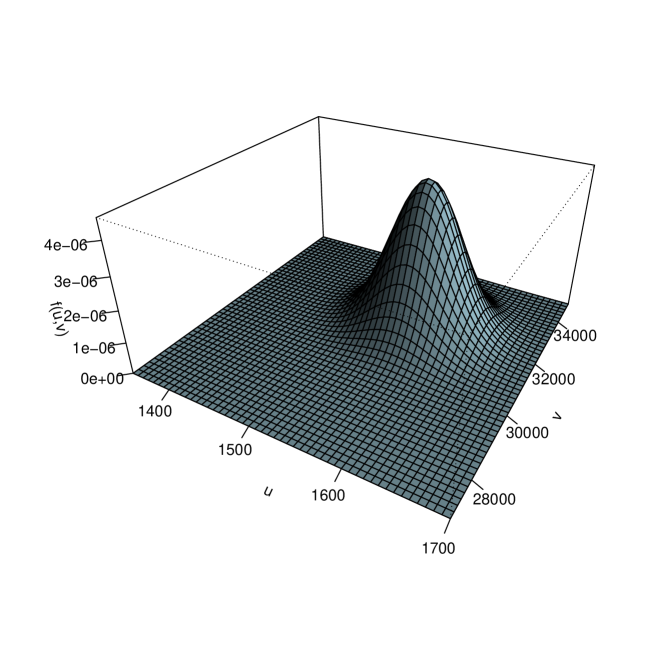
Figure 1: MLE of the Kotz dependent model for the data

Meanwhile, the MLE of the five parameters of the two independent univariate Kotz-gamma distributions of $u$ and $v$, are given as follows:

For the random variable $u$, we have that $\hat{\sigma}_{1}=0.7117504$, $\hat{\alpha}=1472.074$, $\hat{r}=0.5018696$, $\hat{q}=1.000177$ and $\hat{s}=0.9978606$. And for the random variable $v$, we get $\hat{\sigma}_{2}=3.482650$, $\hat{\beta}=1290.797$, $\hat{r}=0.5002108$, $\hat{q}=0.9999866$ and $\hat{s}=1.0005263$. The independent bivariate Kotz gamma distribution is shown in Figure 2.

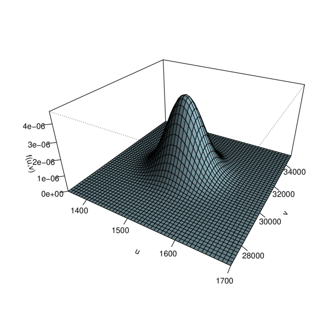
Figure 2: MLE of the Kotz dependent model for the data

By visually comparing the values of the estimators of the parameters of interest, it is clear the importance of establishing whether the random variables under study and their corresponding random samples are independent or not. It is important to note that it is not interesting to compare statistically these values differ from the estimators of the parameters under the two contexts, since they are solutions to different theoretical and/or practical problems.

7 Conclusions

1. The multivector variate distributions, based on multivariate contoured elliptically distribution allow to model joint dependent variables, instead of the usual assumption of independence. Moreover, the use of elliptical models instead of the classical Gaussian, provides a robust way of modeling a number of real situations. Additionally, note that the distributions obtained, in addition to being used as probabilistic models solve the problem of finding the corresponding likelihood functions under independence and dependence.

2. A real data taking from the Colombian financial context verified the importance to determine if the variables under study are independent or not and if the corresponding random samples are also independent or not, since the estimators under the two assumptions are not equal.

3. A number of open problems are of interest, for example, the study of the non central case $\boldsymbol{\mu}\neq\mathbf{0}$ (in (4)) shall allow studied more complex real problems .

References

- Bekker et al. (2011) Bekker, A., Roux, J. J. J., Ehlers, E., Arashi, M. 2001. Bimatrix variate beta type IV distribution: relation to Wilks’s statistics and bimatrix variate Kummer-beta type IV distribution.
- Chen and Novick (1984) Chen, J. J., Novick, M. R., 1984. Bayesian analysis for binomial models with generalized beta prior distributions. J. Educational Statist. 9, 163–175.
- Choi and Wette (1984) Choi, S and Wette, R. 1969. Maximum Likelihood Estimation of the Parameters of the Gamma Distribution and Their Bias. Technometrics, 11(4) 683-69
- Díaz-García, and Gutiérrez-Jáimez (2010a) Díaz-García, J. A., Gutiérrez-Jáimez, R. 2010a. Bimatrix variate generalised beta distributions. South African Statist. J. 44, 193-208.
- Díaz-García, and Gutiérrez-Jáimez (2010b) Díaz-García, J. A., Gutiérrez-Jáimez, R. 2010b. Complex bimatrix variate generalised beta distributions. Linear Algebra Appl. 432 (2-3), 571-582.
- Díaz-García, and Gutiérrez-Jáimez (2011) Díaz-García, J. A., Gutiérrez-Jáimez, R. 2011. Noncentral bimatrix variate generalised beta distributions. Metrika. 73(3), 317-333.
- Dickey (1967) Dickey, J. M. 1967. Matricvariate generalizations of the multivariate - distribution and the inverted multivariate -distribution, Ann. Math.Statist. 38, 511-518.
- Ehlers (2011) Ehlers, R. 2011. Bimatrix variate distributions of Wishart ratios with application. Doctoral dissertation, Faculty of Natural & Agricultural Sciences University of Pretoria, Pretoria. http://hdl.handle.net/2263/31284.
- Fang et al. (1990) Fang, K. T., Kotz, S., Ng, K. W., Symmetric multivariate and related distributions, Springer-Science+Business Media, B.V., New Delhi, 1990.
- Fang and Zhang (1990) Fang, K. T., Zhang, Y. T., Generalized Multivariate Analysis, Science Press, Springer-Verlag, Beijing, 1990.
- Libby and Novick (1982) Libby, D. L., Novick, M. R. (1982) Multivariate Generalized beta distributions with applications to utility assessment. J. Educational Statist. 7, 271–294.
- Muirhead (2005) Muirhead, R. J., 2005. Aspects of Multivariate Statistical Theory. John Wiley & Sons, New York.
- Nadarajah (2007) Nadarajah, S. 2007, A bivariate gamma model for drought. Water Resour. Res. 43, W08501, doi:10.1029/2006WR005641.
- Nadarajah (2013) Nadarajah, S. 2013, A bivariate distribution with gamma and beta marginals with application to drought data. J. App. Statist. 36(3), 277-301.
- Olkin and Liu (2003) Olkin, I., Liu, R., 2003. A bivariate beta distribution. Statist. Prob. Letters, 62, 407–412.
- Sarabia et al. (2014) Sarabia, J. M., Prieto, F., Jordá, V. 2014, Bivariate beta-generated distributions with application to well-being data. J. Statist. Distributions Appl. 1:15. http://www.jsdajournal.com/content/1/1/15.