The Sloan Digital Sky Survey Reverberation Mapping Project: Quasar Host Galaxies at $z<0.8$ from Image Decomposition

Abstract

We present the rest-frame UV and optical photometry and morphology of low-redshift broad-line quasar host galaxies from the Sloan Digital Sky Survey Reverberation Mapping project. Our sample consists of 103 quasars at $z<0.8$, spanning a luminosity range of $-25\leq M_{g}\leq-17$ mag. We stack the multi-epoch images in the $g$ and $i$ bands taken by the Canada-France-Hawaii Telescope. The combined $g$-band ($i$-band) images reach a $5\sigma$ depth of 26.2 (25.2) mag, with a typical PSF size of $0\farcs 7$ ($0\farcs 6$). Each quasar is decomposed into a PSF and a Sérsic profile, representing the central AGN and the host galaxy components, respectively. The systematic errors of the measured host galaxy flux in the two bands are 0.23 and 0.18 mag. The relative errors of the measured galaxy half-light radii ($R_{e}$) are about 13%. We estimate the rest-frame $u$- and $g$-band flux of the host galaxies, and find that the AGN-to-galaxy flux ratios in the $g$ band are between 0.9 to 4.4 (68.3% confidence). These galaxies have high stellar masses $M_{\ast}=10^{10}\sim 10^{11}\,M_{\odot}$. They have similar color with star-forming galaxies at similar redshifts, in consistent with AGN positive feedback in these quasars. We find that the $M_{*}-M_{\text{BH}}$ relation in our sample is shallower than the local $M_{\text{Bulge}}-M_{\text{BH}}$ relation. The Sérsic indices and the $M_{*}-R_{e}$ relation indicate that the majority of the host galaxies are disk-like.

1 Introduction

AGNs are powerful objects where supermassive black holes (SMBHs) in galaxy centers are actively accreting materials, releasing huge amounts of energy by radiation and material outflows. AGNs are believed to have strong impact on their host galaxies, known as AGN feedback (for recent reviews, see Fabian, 2012; King & Pounds, 2015). Such feedback, including “negative feedback” and “positive feedback”, can significantly influence AGN host galaxies in many aspects, especially star formation. The negative feedback scenario suggests that jets and radiative winds from AGN quench star formation by heating and/or expelling cold gas in host galaxies. This scenario provides a possible solution to many key questions in galaxy formation, such as the different shapes between the mass functions of galaxies and dark matter halos at the high mass end. It has been supported by some simulations (e.g., Di Matteo et al., 2005; Springel et al., 2005; Hopkins et al., 2006; Croton et al., 2006). Observations have also found evidence for AGN-driven outflows (e.g., Cicone et al., 2014) and AGN-heated gas around massive quiescent elliptical galaxies (e.g., Spacek et al., 2016). On the contrary, other simulations have shown that the outflow jets may disturb gas in host galaxies, enhancing star formation (e.g., Zinn et al., 2013), which suggests AGN positive feedback. Supporting evidence includes observations that star-forming regions in AGN host galaxies have a significant alignment with jets (e.g., Salomé et al., 2015).

To determine which mechanism dominates, there have been efforts to measure star formation rates (SFRs) and stellar populations in AGN host galaxies. Results from early studies were controversial. For example, Kirhakos et al. (1999) claimed that quasar host galaxies had bluer colors than normal galaxies, suggesting active star formation. McLure et al. (1999) showed that quasar host galaxies had old stellar populations, indicating low recent SFRs. AGN feedback is likely a mixture of positive and negative feedback (e.g., Zinn et al., 2013), and the feedback process can be dominated by either of the mechanisms. In addition, the properties of quasar host galaxies may also depend on redshift and luminosity, which makes the situation more complex.

Large-area sky surveys, such as the Sloan Digital Sky Survey (SDSS; York et al., 2000), have significantly contributed to the study of quasar/AGN host galaxy properties in the past two decades. A commonly used method to study the AGN impact is to analyze the stellar populations of host galaxies. Several recent studies suggest that the host galaxies of unobscured broad-line AGN are massive and systematically bluer than normal galaxies (e.g., Jahnke et al., 2004; Trump et al., 2013), although this result may be largely due to sample selection effects (e.g., Aird et al., 2012). It has also been recognized that AGN feedback may strongly depend on many properties of AGNs. For example, Kauffmann et al. (2003) studied type-II AGNs from SDSS and found that these AGNs were almost exclusively hosted by massive galaxies with stellar mass $M_{*}>10^{10}M_{\odot}$. They also reported that the host galaxies of low-luminosity type-II AGNs had stellar populations similar to early type galaxies, while the host galaxies of high-luminosity AGNs had much younger stellar populations. Hickox et al. (2009) examined a sample of 585 AGNs and concluded that the hosts of radio AGNs were located in “the red sequence”, X-ray selected AGNs were located in “the green valley”, and infrared selected AGNs were bluer than X-ray selected quasars. The dependence of host galaxy properties on AGN types and properties indicates that it is necessary to have thorough studies on all types of AGNs.

For the most luminous AGNs, i.e., unobscured (Type-I) quasars, the measurement of host galaxies is difficult, and often subject to large uncertainties due to the contamination from the quasar light. Currently there are three techniques that are widely used to study quasar host galaxies: spectra energy distribution (SED) fitting, image decomposition, and spectra decomposition. Unlike SED fitting and spectra decomposition, image decomposition does not depend on spectra/SED models of quasars and galaxies. The only major assumption is that the quasar component can be modeled as a point spread function (PSF). Image decomposition can provide the morphological information of host galaxies which can be used to constrain quasar triggering models (e.g., Cisternas et al., 2011; Villforth et al., 2017).

Early studies of AGN image decomposition mainly used Hubble Space Telescope images (e.g., Bahcall et al., 1997; Kirhakos et al., 1999; Jahnke et al., 2004; Kim et al., 2008; Villforth et al., 2017). These samples were usually small. Image decomposition studies using ground-based data can have samples of several hundred of quasars. For example, Matsuoka et al. (2014) performed image decomposition for a sample of $\sim 800$ quasars at $z<0.6$ from the SDSS Stripe 82. The typical PSF size of their images is about $1\farcs 0-1\farcs 1$. They suggested that quasar host galaxies are systematically bluer than normal galaxies. Meanwhile, the systematic errors introduced by the decomposition procedure are poorly understood. For example, Bettoni et al. (2015) fitted the Stripe 82 images of low-redshift SDSS quasars using a different method, and found that quasar host galaxies have similar colors compared to a redshift-matched sample of inactive galaxies, in contrary to the results of Matsuoka et al. (2014).

In order to obtain reliable measurements on quasar host galaxies, high-quality images are needed. In this work, we use deep images from the SDSS Reverberation Mapping (SDSS-RM) project to study 103 quasar host galaxies at $z<0.8$. Our combined $i$-band images reach a $5\sigma$ depth of $>25$ mag with a PSF FWHM of $\sim 0\farcs 6$. The depth and PSF of our images, two crucial factors for the image decomposition analysis, are significantly better than those of the ground-based images in most previous studies. Our paper is organized as follows. Section 2 describes the imaging and spectral data, and the quasar sample in our work. Section 3 presents our image decomposition method. A spectroscopic analysis method that makes use of the result from the image decomposition is discussed in Section 4. Section 5 presents the results, Section 6 presents some further discussions, and Section 7 summarizes this paper. We use a $\Lambda$-dominated flat cosmology with $H_{0}=70$ km s^-1 Mpc^-1, $\Omega_{m}=0.3$, and $\Omega_{\Lambda}=0.7$. We use AB magnitude (Oke & Gunn, 1983) through this paper.

2 Data and Quasar Sample

Table 1: Co-added Imaging Data

Pointing	A	B	C	D	E	F	G	H	I
R.A.	14${}^{\text{h}}14^{\text{m}}51^{\text{s}}$	14${}^{\text{h}}14^{\text{m}}51^{\text{s}}$	14${}^{\text{h}}08^{\text{m}}47^{\text{s}}$	14${}^{\text{h}}08^{\text{m}}19^{\text{s}}$	14${}^{\text{h}}08^{\text{m}}39^{\text{s}}$	14${}^{\text{h}}14^{\text{m}}52^{\text{s}}$	14${}^{\text{h}}21^{\text{m}}03^{\text{s}}$	14${}^{\text{h}}21^{\text{m}}24^{\text{s}}$	14${}^{\text{h}}20^{\text{m}}54^{\text{s}}$
Decl.	52∘05′28′′	52∘06′35′′	52∘09′27′′	53∘05′13′′	54∘01′20′′	54∘04′09′′	54∘01′35′′	53∘05′30′′	52∘09′28′′
$\text{N}_{\text{image},g}$	157	101	97	97	92	91	91	94	99
$\text{N}_{\text{image},i}$	114	74	70	70	68	69	70	70	70
PSF FWHM ($g$)(′′)	0.69	0.72	0.72	0.72	0.73	0.72	0.70	0.71	0.72
PSF FWHM ($i$)(′′)	0.55	0.56	0.57	0.56	0.58	0.57	0.57	0.56	0.57
Mag Limit ($g$)	26.4	26.1	26.2	26.2	26.1	26.1	26.2	26.2	26.2
Mag Limit ($i$)	25.4	25.2	25.3	25.3	25.2	25.2	25.2	25.3	25.2

Notes. All magnitude limits are $5\sigma$ for point sources.

2.1 Imaging and Spectroscopic Data

In this study, we use the optical images and spectra from the SDSS-RM project to analyze quasar host galaxies. We first decompose the $g$- and $i$-band images of each quasar into a PSF component and a Sérsic profile component. Based on the flux ratio of the two components, the spectrum of a quasar is decomposed into an AGN component and a galaxy component. The AGN component is described as the combination of a power-law continuum and emission lines. The rest-frame flux of the host galaxy is then calculated using the galaxy component of the spectrum. We apply this method to analyze host galaxy properties, rather than simply adopting the flux from the image decomposition, because we do not have enough bands to perform the traditional $k$-correction. We will describe the details later.

As part of the SDSS-III program (Eisenstein et al., 2011), SDSS-RM is a multi-object reverberation mapping project, monitoring 849 broad-line quasars in a 7 deg² field. It aims to detect the time lag between the continuum and the broad line region variabilities of quasars, using both spectroscopic and photometric observations. In this study, we use the co-added optical images and spectra. The spectroscopy was made by the Baryonic Oscillation Spectroscopic Survey (BOSS) spectrograph mounted on the SDSS 2.5m telescope (Gunn et al., 2006), which provides a wavelength coverage from 3650 to 10,500 Å and a resolution $R\sim 2000$ (Smee et al., 2013). The photometric monitoring of SDSS-RM was done at the Steward Observatory Bok telescope, the Kitt Peak National Observatory (KPNO) 4m telescope, and the Canada-France-Hawaii Telescope (CFHT). The observations were conducted in 2014, with a cadence of about 2 days in the $g$ and $i$ bands.

In this work, we use images taken by the CFHT using the MegaCam instrument that consists of 36 CCD chips with a pixel scale of $0\farcs 187$ (Aune et al., 2003). The CFHT images have excellent PSFs ($\sim 0\farcs 6$ in the $i$ band), which are much better than the images taken by the other two telescopes. To cover the entire SDSS-RM field, a total of 9 pointings were used (denoted as points A to I; Table 1), and the images at each pointing consist of two dither positions to cover CCD gaps. The detailed information about the observations can be found in Shen et al. (2015a). There are 1067 images in the $g$ band and 794 images in the $i$ band. The typical integration time per exposure is 78 s in $g$ and 111 s in $i$.

2.2 Image Co-addition

In this section, we present our image co-addition method. We first reject images that have poor quality recorded in the observation logs. We further remove cosmic rays from the images using the LA-Cosmic algorithm (van Dokkum, 2001).

2.2.1 Image Selection and Co-addition

For each image, we first estimate three parameters: atmospheric extinction (or sky transparency), PSF FWHM, and sky background. We run SExtractor (Bertin & Arnouts, 1996), and select bright and isolated point sources. The transparency and PSF FWHM are estimated from the photometry and FWHM values of these objects. The sky background is the median value of the image. We then reject images with PSF FWHM values among the largest 10%, images with sky background among the largest 5%, and images with atmospheric extinction among the largest 5%. The typical number of the remaining images at one pointing is $\sim 100$ in the $g$ band and $\sim 70$ in the $i$ band. We utilize a “weighted average” co-addition. Following the method used for the SDSS Stripe 82 image co-addition (Annis et al., 2014; Jiang et al., 2014), each image is assigned a weight proportional to $T/(\text{FWHM}^{2}\sigma^{2})$, where $T$ is the sky transparency, FWHM is the PSF FWHM, and $\sigma$ is the background noise. Since the background noise is dominated by the Poisson noise of sky background in our images, we assume $\sigma^{2}$ is proportional to sky background. We use SWarp (Bertin et al., 2002) to perform the co-addition.

2.2.2 Quality of Co-added Images

Image decomposition of quasar host galaxies requires high image quality. Our co-added images have great depth and PSF compared to the ground-based images in previous studies. The typical $5\sigma$ depth is $26.2$ mag in $g$ and $25.2$ mag in $i$ for point sources. They are about one magnitude deeper than the combined SDSS Stripe 82 images. The PSF FWHM values of our images are about $0\farcs 7$ and $0\farcs 6$ in the $g$ and $i$ bands, respectively. The variation of the PSF FWHM across an image is small. Over the entire SDSS-RM field, the variation is less than 15%. Note that images with the largest 5% PSFs have been removed earlier. The PSF variation will be taken into account in the image decomposition process. More information about co-added images is listed in Table 1.

2.3 Quasar Sample

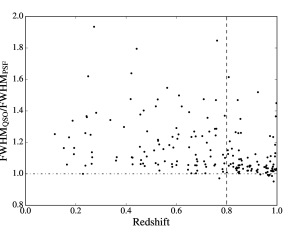
Figure 1: The distribution of the quasar redshifts and FWHM. Quasars with $\text{FWHM}_{\text{QSO}}/\text{FWHM}_{\text{PSF}}>1$ are likely to have resolved host galaxy components. The dashed line indicates our redshift cut $z<0.8$.

The SDSS-RM quasar sample consists of 849 quasars with $i<21.7$ mag. To estimate the redshift range in which quasars are resolved in our images, we examine the relation between the redshifts and the FWHM of the quasar images. Figure 1 shows the relation in the $i$ band. Most quasars at $z<0.8$ have FWHM larger than the PSF FWHM in both $g$ and $i$ bands, so we select quasars at $z<0.8$ to construct our sample. This ensures a high success rate for image decomposition. There are a total of 105 $z<0.8$ quasars in the SDSS-RM sample. We visually inspect all these quasars, and exclude two quasars that are blended with nearby objects, or located at image edges. Our final sample consists of 103 quasars at $z<0.8$. The distributions of their redshifts and $g$-band absolute magnitudes are shown in Figure 2. More than half of the quasars are at $z>0.5$.

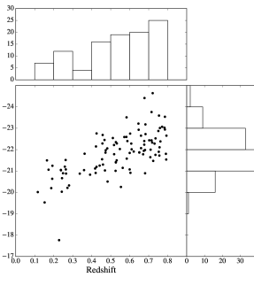
Figure 2: The distribution of the redshifts and the $g$-band absolute magnitudes $M_{g}$ of the 103 quasars in our sample.

3 Image Decomposition and Simulations

3.1 Image Analysis

In the following text, we use “AGN component” and “galaxy component” to denote the central AGN (point source) and the host galaxy, respectively. Meanwhile, a “quasar” refers to the whole system, including the AGN and its host galaxy.

For each quasar, we decompose its image into a PSF (the AGN component) and a Sérsic profile (the galaxy component). Our procedure is similar to Matsuoka et al. (2014). We first resample the image so that the quasar center is located in the center of a pixel. The pixel scale is reserved. A local background is measured and subtracted. The PSF map of each image is modeled by PSFEx (Bertin, 2011). PSFEx selects bright point sources according to their half-light radii and flux, and fits PSFs to these sources. The output of PSFEx is a PSF map of a polynomial function of positions. More information about PSF modeling can be found in Appendix A. The PSF of a quasar is determined based on its position in the image. The PSF component has one free parameter, its flux. The Sérsic function (Sersic, 1968) describes the radial profile of a galaxy and has the form

$$I(r)=I_{e}\times\text{exp}\{-b_{n}[(\frac{r}{R_{e}})^{\frac{1}{n}}-1]\},$$ (1)

where $n$ is the Sérsic index that determines the shape of the profile, and $R_{e}$ is the effective radius that includes half of the total galaxy flux. By this definition, we can determine $b_{n}$ as a function of $n$. Therefore, a Sérsic profile has three free parameters: $I_{e}$, $R_{e}$ and $n$. A Gaussian profile has $n=1/2$, an exponential disk has $n=1$, and a de Vaucouleurs profile has $n=4$. Most galaxies have $0.5<n<5$. The Sérsic profile is convolved with the PSF to model the galaxy image.

We fit the 1-dimensional (1-D) radial profile of each quasar. The radial profile $I(j)$ at the $j$th data point is the mean value of all pixels whose distances to the object center $r$ satisfy $j-1<r\leq j$. Data points with $1\leq j\leq 10$ in the 1-D profiles are fitted. The central pixel $j=0$ is excluded in the fitting process, because the error of the PSF model is usually large in the center. We fit the image by minimizing the $\chi^{2}$ value defined as

$$\chi^{2}=\sum_{j}\frac{[I(j)-I_{P}P(j)-I_{G}G(j,R_{e},n)]^{2}}{\sigma_{j}^{2}},$$ (2)

where $P(j)$ is the 1-D profile of the flux-normalized PSF, $G(j,R_{e},n)$ is the 1-D profile of the flux-normalized model galaxy image, $I_{P}$ and $I_{G}$ are the intensities of PSF and galaxy components, and $\sigma_{j}$ is the uncertainty of the $j$th data point. The uncertainty is calculated by $\sigma_{j}^{2}=\sigma_{b,j}^{2}+\text{DN}_{j}/gain$, where $\sigma_{b,j}$ is the background noise at pixel $j$, DN_j is the digital number of pixel $j$, and $gain$ is the gain of the image in e^-/ADU.

The fitting procedure involves four parameters: $I_{P}$, $I_{G}$, $R_{e}$, and $n$. We allow $R_{e}$ to vary from 0.5 to 10.0 pixels with a step of 0.1 pixels, and $n$ to vary from 0.1 to 5.0 with a step of 0.1. For each pair of $R_{e}$ and $n$, we calculate $I_{P}$ and $I_{G}$ using $\partial{\chi^{2}}/\partial{I_{P}}=0$ and $\partial{\chi^{2}}/\partial{I_{G}}=0$ to minimize $\chi^{2}$. For each quasar, we first fit the $i$-band image to obtain the best-fitted $n$ and $R_{e}$ values. We then fix the $n$ and $R_{e}$ values for the $g$-band image decomposition. This is because the $i$-band images have smaller PSF, and host galaxies are relatively brighter in the $i$ band. Figure 3 shows an example of decomposition. We use the PSF-subtracted images as the best-fitted host galaxy images. The flux of quasars and galaxies is measured in a $2\arcsec$ aperture, corresponding to the fiber diameter of the BOSS spectrograph. The magnitudes, colors, and stellar masses of the quasar host galaxies that we discuss in Section 6 are all based on the $2\arcsec$ aperture flux. As primary results, quasar host galaxies in our sample have $g-i$ color $\sim 0.5-2.5$, half-light radius $R_{e}\sim 0\farcs 3-1\farcs 4$ and Sérsic index $n\sim 0.5-3$.

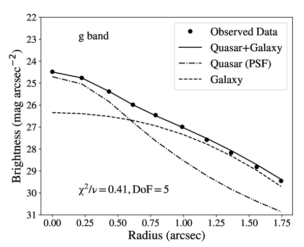
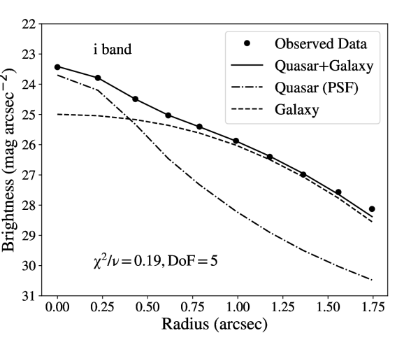
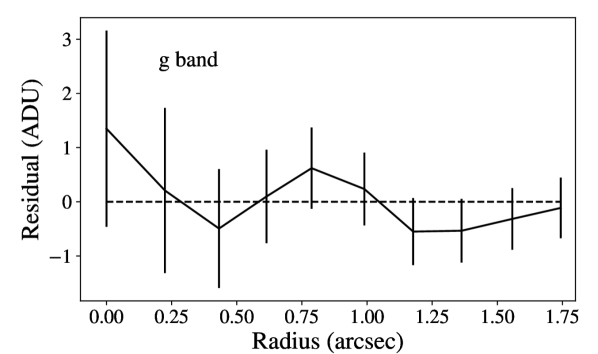
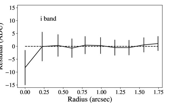
Figure 3: An example of image decomposition for quasar ID 338 in our sample. Upper Panel: the decomposed images. The images are shown in the RGB color mode where the $i$-band images are shown in the R channel, the $g$-band images are shown in the G channel, and the B channel shows nothing. From left to right: the original image, the PSF component, and the PSF-subtracted image. The pixel scale of the images is 0.187”/pixel. Middle panels: The 1-D image decomposition process in the $g$ and $i$ bands. The black dots are the measured 1-D profile of the object. The black solid line is the best-fitted 1-D profile. The dashed and dot-dashed lines are the best-fitted profiles of the host galaxy and the AGN components, respectively. The error bars are very small comparing to the scale of the plot, and they are not shown in this panel for clarity. Lower Panels: The residuals of the 1-D profile fitting in the two bands.

3.2 Comparison to Simulations

We assess our decomposition method using simulations. We use extended objects in our fields, selected from the SDSS photometric catalog, to mimic galaxy components, and point sources in the fields to mimic AGN components. The science and noise images of these sources are scaled to match the desired galaxy and AGN flux. Then these images are combined to make simulated quasar images. To ensure that the mock “galaxies” and “AGNs” can be accurately described by Sérsic profiles and PSF models, we run the fitting process in Section 3.1 on the mock “galaxies” and “AGNs”. Only “pure galaxies” with $|m_{\text{S\'{e}rsic}}-m_{\text{galaxy}}|<0.1$ and “pure AGNs” with $|m_{\text{PSF}}-m_{\text{AGN}}|<0.1$ are selected for the following analysis.

For the convenience of further discussion, we define several terms and symbols using the $g$ band as an example. We use $f^{g}_{\text{gal,\,raw}}$ ($f^{g}_{\text{AGN,\,raw}}$) to denote the flux of extended (point) sources in the $g$ band in the original images, and use $f^{g}_{\text{gal}}$ ($f^{g}_{\text{AGN}}$) to denote the flux that is scaled to match the desired galaxy and AGN flux. We use $R^{g}_{\text{gal}}$ to represent the galaxy-to-total flux ratio in the $g$ band, $R^{g}_{\text{gal}}=f^{g}_{\text{gal}}/f^{g}_{\text{total}}$, where $f^{g}_{\text{total}}=f^{g}_{\text{gal}}+f^{g}_{\text{AGN}}$. We define $f^{g}_{\text{AGN,\,fit}}$ as the best-fitted flux of the PSF component. The fitting results of galaxies are more complex. There are two types of the fitted flux: one is the flux of the model Sérsic profile, which is referred to as $f^{g}_{\text{gal,\,S\'{e}rsic}}$. The other one is the residual flux after the subtraction of the best-fitted PSF component, which is referred to as $f^{g}_{\text{gal,\,fit}}$, i.e., $f^{g}_{\text{gal,\,fit}}=f^{g}_{\text{total}}-f^{g}_{\text{AGN,\,fit}}$. Accordingly, we define the “fitted” galaxy-to-total ratio as $R^{g}_{\text{gal,\,fit}}=f^{g}_{\text{gal,\,fit}}/f^{g}_{\text{total}}$.

We first construct a parent sample of simulated host galaxies in the $i$ band. We generate $10^{4}$ sets of [$m^{i}_{\text{total}},R^{i}_{\text{gal}}$] values so that $m^{i}_{\text{total}}$ is uniformly distributed between 17 and 23 mag and $R^{i}_{\text{gal}}$ is uniformly distributed between 0 and 1. For each pair of [$m^{i}_{\text{total}},R^{i}_{\text{gal}}$], we calculate $f^{i}_{\text{gal}}$ and $f^{i}_{\text{AGN}}$, and select one extended source and one point source that satisfy $|f^{i}_{\text{gal,raw}}-f^{i}_{\text{gal}}|<0.1\times f^{i}_{\text{gal}}$ and $|f^{i}_{\text{AGN,raw}}-f^{i}_{\text{AGN}}|<0.1\times f^{i}_{\text{AGN}}$. Then the two images are scaled so that the flux of the two sources equals $f^{i}_{\text{gal}}$ and $f^{i}_{\text{AGN}}$, respectively. By doing this, the scaling factors are close to 1, and the noise of simulated images are close to that of the real data. The extended sources for the simulated $g$-band images and their scaling factors are the same as those for the simulated $i$-band images. The $g$-band flux of the simulated AGN component, $f^{g}_{\text{AGN}}$, is generated so that the $g-i$ colors of simulated objects follow the $g-i$ color distribution of our quasar sample. The selection method is the same as for the $i$-band images. Finally, the images of extended sources and point sources are combined to create the simulated quasar images.

To mimic the real quasar host galaxy sample, we select a subset of the parent sample of simulated quasar host galaxies which satisfies (1) the distribution of $R_{\text{gal}}$ is the same as that for the real sample, (2) the distribution of the total flux ($f_{\text{total}}=f_{\text{gal}}+f_{\text{AGN}}$), or the total magnitude ($m_{\text{total}}$), is the same as the real sample, and (3) the distribution of the $g-i$ colors (i.e., $m^{g}_{\text{total}}-m^{i}_{\text{total}}$) is the same as the real sample. The fitting uncertainties are sensitive to the galaxy flux and $R_{\text{gal}}$. The simulated sample is used to provide a solid measurement of uncertainties in the fitting process.

We define “Successful Fitting Criteria” as follows:

(1) Best-fitted Sérsic index $n>0.1$.

(2) Best-fitted half-light radius $R_{e}>1$ pixel.

(3) $(f_{\text{gal,\,S\'{e}rsic}}-f_{\text{gal,\,fit}})^{2}<0.1\times(f_{\text{gal,\,fit}})^{2}$ in both $g$ and $i$ bands.

These requirements are set because of the following reasons. First, an object with $n=0.1$ usually has a very faint galaxy component, because the shape of an $n=0.1$ Sérsic profile is a flat disk at $r<R_{e}$. In this case, the best-fitted “galaxy component” is likely the residual of background subtraction. Second, an object with $R_{e}\leq 1$ pixel are usually not resolved. Finally, an object with $(f_{\text{gal,\,S\'{e}rsic}}-f_{\text{gal,\,fit}})^{2}>0.1\times(f_{\text{gal,\,fit}})^{2}$ (i.e., the flux of the model Sérsic profile is very different from the total flux minus the PSF component flux) usually has an unusual morphology which cannot be well described by a Sérsic profile. Objects that do not satisfy the criteria have large flux fitting error in our simulation and are rejected in the further analysis. 95 out of 103 quasars in our sample meet the “Successful Fitting Criteria”.

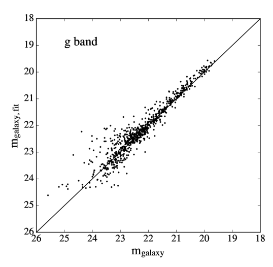
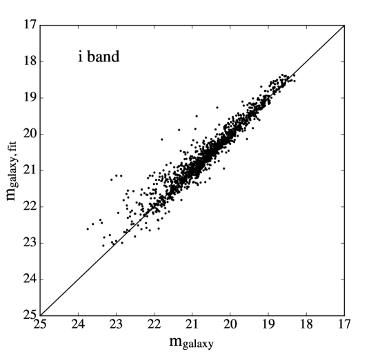
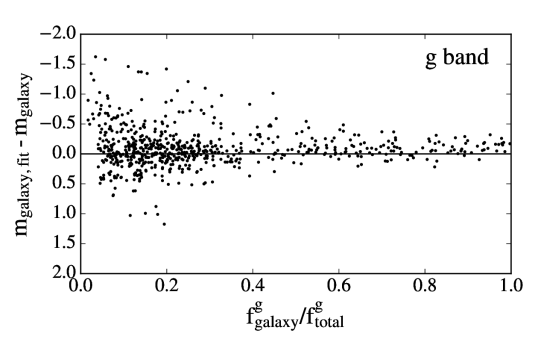
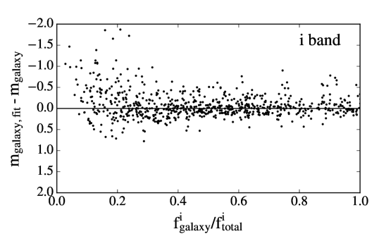
Figure 4: Estimating the fitting errors of the galaxy magnitudes. $Upper$ $Panel:$ Comparison between the real magnitudes and fitted magnitudes of the galaxy components in the simulated quasar host galaxy sample. Our fitting technique produces $\Delta m^{g}_{\text{galaxy}}=-0.04\pm 0.23$ and $\Delta m^{i}_{\text{galaxy}}=-0.02\pm 0.18$. $Lower$ $Panel:$ The influence of the galaxy-to-total flux ratios on the fitting errors. At $f^{i}_{\text{galaxy}}/f^{i}_{\text{total}}>0.1$, there is no evidence that the fitting error evolves with the galaxy-to-total flux ratio, while for objects with $f^{i}_{\text{galaxy}}/f^{i}_{\text{total}}<0.1$, the galaxy flux tends to be slightly overestimated.

Figure 5: Fitting errors of the $g-i$ color of the galaxies. $Left$ $Panel:$ The relation between $f^{i}_{\text{galaxy}}/f^{i}_{\text{total}}$ and host galaxy $g-i$ color error. Our fitting technique yields $\Delta(g-i)_{\text{galaxy}}=-0.03\pm 0.20$. $Right$ $Panel:$ The relation between $m^{i}_{\text{galaxy}}$ and host galaxy $g-i$ color error. Neither galaxy flux nor galaxy-to-total flux ratio shows obvious influence on the systematic errors of the galaxy color measurement.

This work focuses on the luminosities, colors, and morphologies of the quasar host galaxies. We estimate the fitting errors of galaxy magnitudes, colors, half-light radii and Sérsic indices here. Since the distributions of the errors are not Gaussian, we use the so-called “robust statistical estimators”, i.e., the biweight location and the biweight scale (Beers et al., 1990). In short, the biweight location and the biweight scale are counterparts of mean and standard deviation but are less sensitive to outliers. In the following text, the expression $\Delta A=\overline{\Delta A}\pm\sigma_{A}$ means that the fitting error $\Delta A$ of a quantity $A$ has a biweight location of $\overline{\Delta A}$ and a biweight scale of $\sigma_{A}$. For the successfully fitted objects, the simulation produces $\Delta m_{i}=-0.02\pm 0.18$ and $\Delta m_{g}=-0.04\pm 0.23$. The systematic flux errors are much smaller than the random errors. Figure 4 shows the comparison between the real and fitted magnitudes of galaxies in the $g$ and $i$ bands. It demonstrates that the systematic fitting errors evolve little with the galaxy-to-total flux ratios $R_{\text{gal}}\equiv f_{\text{gal}}/f_{\text{total}}$. For objects with $R^{g}_{\text{gal}}<0.05$ or $R^{i}_{\text{gal}}<0.1$, our image decomposition tends to overestimate the galaxy flux by $\sim 1$mag. A similar trend was also reported in Matsuoka et al. (2014). Therefore, the estimated flux at $R^{i}_{\text{gal,fit}}\lesssim 0.2$ may suffer larger systematic flux errors, comparing to the rest of the sample. There are 8 out of 103 quasars which have $R^{i}_{\text{gal,fit}}<0.2$. We will estimate the typical flux errors of $R^{i}_{\text{gal,fit}}<0.2$ quasars and $R^{i}_{\text{gal,fit}}>0.2$ quasars respectively in Section 4.2.

Figure 5 presents the systematic errors of the host galaxy $g-i$ colors and their dependence on galaxy flux and $R_{\text{gal}}$. Our sample gives $(g-i)_{\text{gal,\,fit}}-(g-i)_{\text{gal,\,real}}=-0.03\pm 0.20$. Either galaxy flux or $R_{\text{gal}}$ has no obvious systematic impact on the measured galaxy colors.

Figure 6 illustrates the influence of the quasar-to-PSF FWHM ratios ($\text{FWHM}_{\text{QSO}}/\text{FWHM}_{\text{PSF}}$) on the fitting error of the galaxy flux. The random errors increase with decreasing $\text{FWHM}_{\text{QSO}}/\text{FWHM}_{\text{PSF}}$, as expected. No significant systematic errors can be seen. Most outliers in the flux error distribution appear at $\text{FWHM}_{\text{QSO}}/\text{FWHM}_{\text{PSF}}<1.05$ in both bands. We compare the distribution of $\text{FWHM}_{\text{QSO}}/\text{FWHM}_{\text{PSF}}$ of the simulated sample with that of the real quasar sample. We use the biweight location and scale to estimate the distribution of $\text{FWHM}_{\text{QSO}}/\text{FWHM}_{\text{PSF}}$. The object-to-PSF FWHM ratios in the $i$ band are $1.17\pm 0.17$ for the real sample and $1.15\pm 0.17$ for the simulated sample. In the $g$ band, the two values are $1.05\pm 0.05$ and $1.05\pm 0.05$, respectively. These results indicates that the real and simulated samples have similar object-to-PSF FWHM ratios, and thus our error estimation is reliable.

Figure 7 shows the errors of the best-fitted Sérsic parameters. Our decomposition method yields $n_{\text{fit}}/n_{\text{real}}=1.06\pm 0.39$ and $R_{e,\text{fit}}/R_{e,\text{real}}=1.03\pm 0.13$. Although the uncertainties of Sérsic indices are relatively large, the distribution of $n_{\text{fit}}$ is similar to that of $n_{\text{real}}$ (Figure 8), which is useful for analyzing the overall quasar host galaxy population.

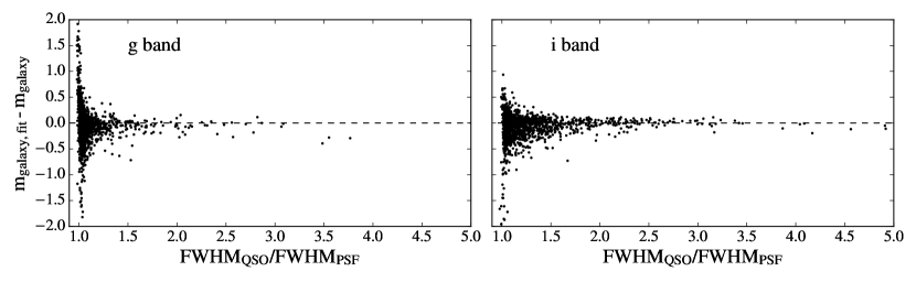
Figure 6: The influence of the $\text{FWHM}_{\text{QSO}}/\text{FWHM}_{\text{PSF}}$ on the fitting error of the galaxy flux. The flux errors increase towards small $\text{FWHM}_{\text{QSO}}/\text{FWHM}_{\text{PSF}}$. Outliers with large fitting flux error appear at $\text{FWHM}_{\text{QSO}}/\text{FWHM}_{\text{PSF}}<1.05$ for both bands.

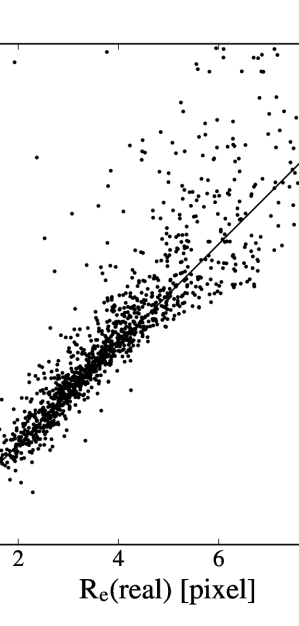
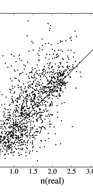
Figure 7: Fitting errors of the Sérsic parameters of galaxies in the $i$ band. Random offsets are added to the points to make them distinguishable in the grid. $Left$ $Panel:$ half-light radius $R_{e}$, with $R_{e,\text{fit}}/R_{e,\text{real}}=1.03\pm 0.13$. $Right$ $Panel:$ Sérsic index $n$, with $n_{\text{fit}}/n_{\text{real}}=1.06\pm 0.39$.

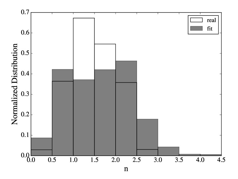
Figure 8: The distribution of “real” and “fitted” Sérsic indices of the simulated quasar host galaxies. The two distributions are roughly consistent.

3.3 Comparison with Previous Work

Our image decomposition method is similar to the method used by Matsuoka et al. (2014), who analyzed the SDSS Stripe 82 images with PSF FWHM $\sim 1\farcs 1$, and fitted the 1-D profiles of quasar host galaxies in the five SDSS bands. They first fitted the $i$-band images, then fitted images in the other bands assuming that the Sérsic parameters ($R_{e}$ and $n$) were the same in all five bands. To avoid parameter degeneracy, they fitted the quasar images in two steps. First, the PSF component was fitted assuming that central pixels within $r<2$ pixels are solely produced by the PSF component. The Sérsic parameters were fitted after PSF component was subtracted from the original image. Their simulations gave $\Delta m_{g}=-0.08\pm 0.63$ and $\Delta m_{i}=0.02\pm 0.49$. There was a clear trend in their simulation that, for host galaxies with small $R_{\text{gal}}$, the fitted galaxy flux was overestimated. They suggested that their data were not suitable to study host galaxy morphology, and did not compare the “real” and “fitted” Sérsic parameters of their simulated quasar host galaxies.

In our work, we fit the four parameters ($I_{P},I_{G},R_{e},n$) simultaneously. According to simulation, we set up “Successful Fitting Criteria” to exclude objects with large fitting error. For objects that satisfy the criteria, the fitting errors are $\Delta m^{g}_{\text{galaxy}}=-0.04\pm 0.23$, $\Delta m^{i}_{\text{galaxy}}=-0.02\pm 0.18$, $R_{e,\text{fit}}/R_{e,\text{real}}=1.03\pm 0.13$ and $n_{\text{fit}}/n_{\text{real}}=-0.04\pm 0.23$. Our fitting process overestimates galaxy flux for objects which have $R^{g}_{\text{gal}}<0.05$ or $R^{i}_{\text{gal}}<0.1$.

4 Spectroscopic Analysis

Traditionally, a $k$-correction is used to convert observed magnitudes to rest-frame magnitudes. However, this approach does not work well with only two magnitudes. We introduce a method that can estimate the rest-frame flux of quasar host galaxies, using the results of the image decomposition and the high-SNR quasar spectra from the SDSS-RM program.

We use the combined multi-epoch spectra from the SDSS-RM project. The co-addition strategy can be found in Shen et al. (2015a). Briefly, for each quasar, the spectra of 32 epochs were co-added with an inverse-variance weight. The total exposure time of each co-added spectrum is roughly 65 hr. We then correct for Galactic extinction using the dust map from Schlegel et al. (1998) and the Galactic extinction curve from Cardelli et al. (1989). The spectrum of one quasar was severely affected by bad pixels and is rejected.

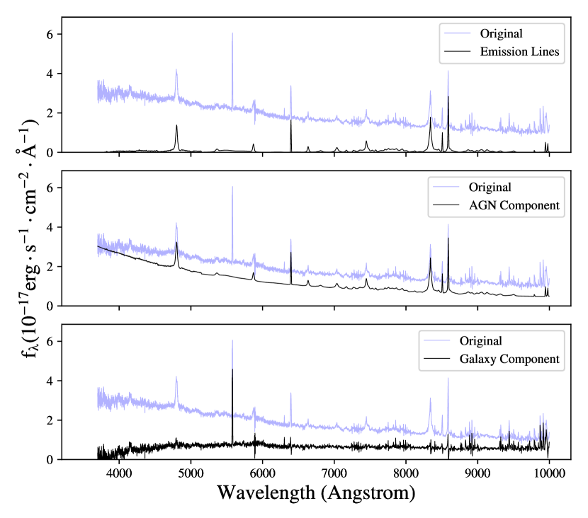
Figure 9: An example of quasar host galaxy spectrum fitting (RMID=33). Upper Panel: Fitting emission lines. The blue line is the original spectrum and the black line is the fitted emission line component. Middle Panel: The modelled AGN component spectrum. Assuming that the AGN spectrum is a power law continuum plus the emission line component, the power law continuum is determined by the AGN-to-total flux ratio in $g$ and $i$ band obtained from image decomposition. The black line shows the modelled AGN spectrum (power-law continuum plus emission lines). Lower Panel: The modelled galaxy spectrum, which is the original spectrum minus the modelled AGN component spectrum.

4.1 Method

The basic idea is to model the AGN component so that the AGN-to-total flux ratios in the observed $g$ and $i$ bands are equal to the values from the image decomposition. We assume that the AGN component is described as a power-law continuum plus emission lines,

$$f_{\text{AGN}}(\lambda)=A\lambda^{\alpha}+f_{\text{lines}}(\lambda)$$ (3)

where the flux of the emission lines, $f_{\text{lines}}(\lambda)$, can be measured by fitting the spectrum. Under this assumption, the AGN-to-total flux ratio, $R^{g}_{\text{AGN}}=f^{g}_{\text{AGN}}/f^{g}_{\text{total}}$, is a function of $A$ and $\alpha$. Solving the equation set

$$\left\{\begin{array}[]{lr}R^{g}_{\text{AGN}}(A,\alpha)&=R^{g}_{\text{AGN}}(\text{image decomposition})\\ R^{i}_{\text{AGN}}(A,\alpha)&=R^{i}_{\text{AGN}}(\text{image decomposition})\end{array}\right.$$ (4)

gives $A$ and $\alpha$, and thus the AGN spectrum. The galaxy spectrum is obtained by subtracting the AGN spectrum from the total spectrum, and the rest-frame galaxy flux is calculated accordingly. Given the wavelength range of the SDSS-RM spectra, we are able to measure the rest-frame $u$ and $g$ flux for quasars at $0.2<z<0.8$.

To get the emission line flux, we fit a rest-frame range 2000 $\sim$ 7200 Å in the spectra of all quasars in our sample. The wavelength range covers the observed $g$ and $i$ band at $0.2<z<0.8$. We fit nine wavelength intervals separately (see below), with each interval fitted as a local power law plus a set of emission lines. Emission lines (except Fe ii lines) are fitted by Voigt profiles. Fe ii lines are modeled by convolving a Gaussian profile with Fe ii templates. We use Fe ii template from Tsuzuki et al. (2006) to fit ultraviolet Fe ii lines (2000 $\sim$ 3500 Å) and template from Véron-Cetty et al. (2004) to fit optical Fe ii lines (3500 $\sim$ 7000 Å). The fitted emission lines include:

(1) 2000$\sim$3000 Å: Mg ii $\lambda 2799$ and Fe ii lines.

(2) 3000$\sim$3500 Å: O ii $\lambda 3134$, He i $\lambda 3188$, [Ne v] $\lambda 3347$, [Ne v] $\lambda 3427$ and Fe ii lines.

(3) 3500$\sim$3900 Å: [O ii] $\lambda 3726$, [Ne iii] $\lambda 3869$ and Fe ii lines.

(4) 3900$\sim$4700 Å: [Ne iii] $\lambda 3967$, H$\delta$, H$\gamma$ and Fe ii lines.

(5) 4700$\sim$5100 Å: H$\beta$, [O iii] $\lambda\lambda 4959,5007$ and Fe ii lines. One narrow component and one broad component are fitted to the H$\beta$ emission.

(6) 5100$\sim$5600 Å: [Cl iii] $\lambda 5538$ and Fe ii lines.

(7) 5600$\sim$6200 Å: He i $\lambda 5876$ and Fe ii lines.

(8) 6200$\sim$6900 Å: H$\alpha$, [N ii] $\lambda 6583$, [S ii] $\lambda\lambda$6716, 6731 lines. One narrow component and three broad component are fitted to the H$\alpha$ emission, since H$\alpha$ emission features in quasars frequently possess complex line profiles.

(9) 6900$\sim$7200 Å: He i $\lambda 7065$.

Figure 9 shows an example of emission line fitting and galaxy spectrum modeling.

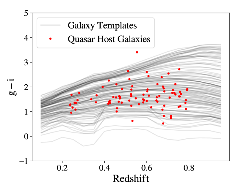
Figure 10: The $g-i$ colors of the galaxy templates used to simulate the “AGN + host” spectra. The grey lines show the observed $g-i$ colors as a function of redshift. The dots represent the quasar host galaxies in our sample. The quasar host galaxies and the galaxy templates occupy roughly the same region in this plot.

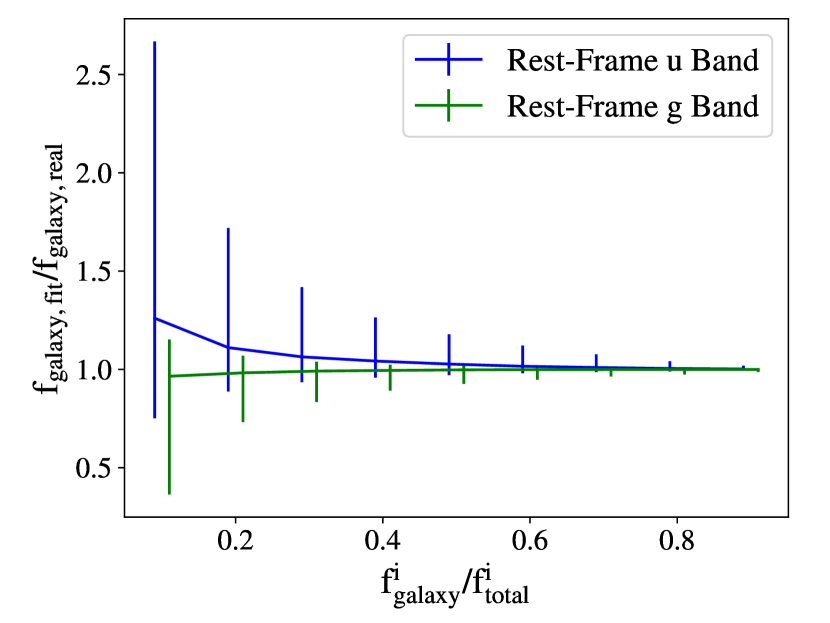
Figure 11: The estimated error of galaxy flux from the spectra analysis. The solid lines illustrate the median value and the error bars shows the range that covers 68% of the simulated spectra. Small offsets are applied on the two lines for the sake of clarity. For objects with $f^{i}_{\text{galaxy}}/f^{i}_{\text{total}}<0.2$, rest-frame $u$ band flux has a large uncertainty and is likely to be overestimated. The error of the rest-frame $g$-band flux is significantly smaller than that of the rest-frame $u$-band flux.

4.2 Error Estimation

We simulate quasar spectra and estimate the errors of the rest-frame galaxy flux introduced by our spectroscopic analysis. We select 12 luminous quasars at $0.2<z<0.8$ from the SDSS DR12 quasar catalog (Pâris et al., 2017) and use their spectra as AGN templates. The details are as follows. We divide the redshift range $0.2<z<0.8$ evenly into 6 redshift bins, with a bin size of $\Delta z=0.1$, and select the brightest two quasars in the $i$ band for each redshift bin. The two quasars at $0.2<z<0.3$ have $i$-band absolute magnitudes around –23.5 mag. The quasars in the other redshift bins have $i$-band absolute magnitudes brighter than $-24.5$ mag. We assume that the host galaxy components in these spectra are negligible. The galaxy templates are from Brown et al. (2014), who provided an atlas of high-SNR spectra of 129 galaxies covering a wavelength range from the rest-frame UV to the mid-IR. We ensure that the colors of the galaxy templates are close to the colors of the quasar host galaxies in our sample. Figure 10 shows the observed $g-i$ colors of the quasar host galaxies in our sample, compared to the observed $g-i$ colors of the galaxy templates. They cover similar parameter space.

We combine the AGN templates and the galaxy templates to generate simulated quasar spectra. For every possible combination of AGN template and galaxy template, we generate 9 simulated spectra, with the observed $R^{i}_{\text{gal}}$ varies from 0.1 to 0.9 with a step of 0.1. The number of simulated spectra is $12\times 129\times 9=13932$. We apply our spectroscopic analysis to these simulated spectra and calculate the rest-frame $u$ and $g$ flux of the galaxies. Figure 11 shows the result of the error estimation. At $R^{i}_{\text{gal}}<0.2$, the rest-frame $u$ band flux is likely to be overestimated, with relatively large errors. This is mainly due to the difficulty in modeling the small blue bump (SBB) at $\sim 3000$Å. When the galaxy component is very faint compared to the AGN component, small errors in modeling the SBB will result in large errors in estimating galaxy flux. At $R^{i}_{\text{gal}}>0.2$, the error of the rest-frame $u$-band flux is comparable to or smaller than the uncertainty from the image decomposition. The median of $f_{\text{gal,\,fit}}/f_{\text{gal,\,real}}$ at $R^{i}_{\text{gal}}>0.2$ is 1.02 in the rest-frame $u$ band, and the standard deviation is 0.27. The biweight scale of $f_{\text{gal,\,fit}}/f_{\text{gal,\,real}}$ in the rest-frame $u$ band is only 0.006, meaning that the large error bars shown in Figure 11 are mainly from outliers. The errors in the rest-frame $g$ band are significantly smaller than those in the rest-frame $u$ band. At $R^{i}_{\text{gal}}<0.2$, the rest-frame $g$ band flux errors are comparable to the errors from image decomposition, and the errors decrease towards larger $R^{i}_{\text{gal}}$ values. At $R^{i}_{\text{gal}}>0.2$, the median of $f_{\text{gal,\,fit}}/f_{\text{gal,\,real}}$ in the rest-frame $g$ band is 0.998, the standard deviation is 0.08, and the biweight scale is 0.0006. Our simulation shows that, though the flux errors of individual quasar host galaxies can be large (especially in the rest-frame $u$ band), the systematic error are small.

Finally, we estimate typical errors from the combination of our image decomposition and spectroscopic analysis. As we discussed earlier, objects with $R^{i}_{\text{gal}}<0.2$ have significantly larger errors than the rest of the sample, so we divide our sample into two subsamples, with $R^{i}_{\text{gal}}<0.2$ and $R^{i}_{\text{gal}}>0.2$. The $R^{i}_{\text{gal}}<0.2$ subsample consists of only 8 quasars, and has large random errors ($\gtrsim 0.5$ mag in both bands). We focus on their median magnitude and color when interpreting our results, and estimate the systematic errors as follows. According to Figure 4, our image decomposition overestimates the flux of these objects by $\sim 0.5$ mag in both observed $g$ and $i$ band, and spectroscopic analysis will further overestimate their rest-frame $u$-band flux by $\sim 0.3$ mag. The net effect is that these objects have their rest-frame $g$-band flux overestimated by $\sim 0.5$ mag, and their rest-frame $u-g$ colors underestimated by $\sim 0.3$ mag.

The $R^{i}_{\text{gal}}>0.2$ subsample does not have significant systematic flux errors. Our simulated sample shows that the uncertainties of the observed $g$- and $i$-band magnitudes are 0.21 and 0.17 mag, respectively. We use 0.2 mag as the typical error of image decomposition. The uncertainty of spectroscopic analysis is negligible, or comparable to the uncertainty from the image decomposition. For the typical error of spectroscopic analysis, we take the standard deviation as a conservative estimate, which is 0.26 mag for the rest-frame $u$ band and 0.08 mag for the rest-frame $g$ band. We then take the quadrature sum of the uncertainties from the two steps as final magnitude uncertainty, which gives $\sigma_{u}=0.33$ and $\sigma_{g}=0.22$ for the two bands. The errors of other properties derived from flux, including the rest-frame $u-g$ colors and stellar masses, are estimated accordingly.

5 Results

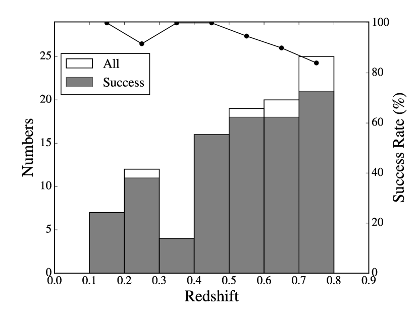
Figure 12: The “success rate” of the image decomposition as a function of redshift. The histogram displays the total number (white) and the number of successfully fitted quasars (gray) in each redshift bin. The filled circles indicate the success rates in individual redshift bins. A total of 88 out of 96 quasars in our $0.2<z<0.8$ sample are successfully fitted. The success rate decreases slowly with redshift, and the success rate at $0.7<z<0.8$ is 84%.

We fit all 103 quasars in our sample, and 95 of them meet the “Successful Fitting Criteria” defined in Section 3.2. Figure 12 shows the success rate as a function of redshift. The success rate decreases slowly with redshift. The success rate at $0.7<z<0.8$ is 84%, which is still high. This indicates that our redshift cut ($z<0.8$) is reasonable. Our optical spectra do not cover the rest-frame $u$ band for quasars at $z<0.2$, so we focus on the quasars at $0.2<z<0.8$. There are 95 quasars in this redshift range, and 87 of them are successfully fitted.

5.1 Flux and Colors of Quasar Host Galaxies

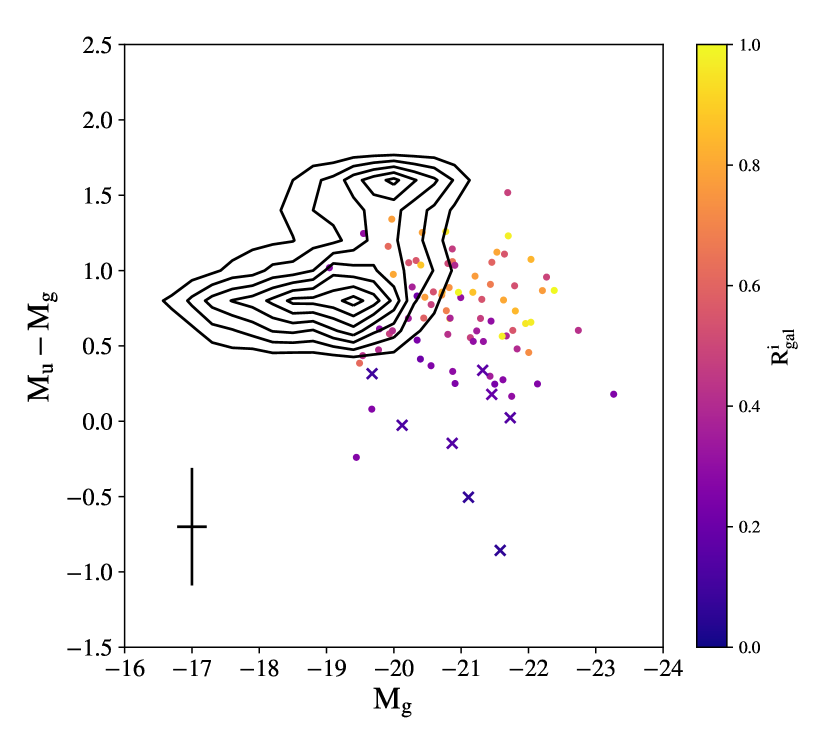
Figure 13: The rest-frame CMD ($M_{g}$ vs $M_{u}-M_{g}$) of the quasar host galaxies. The crosses represent the quasar host galaxies with $R^{i}_{\text{gal}}<0.2$, and the black dots represent the host galaxies with $R^{i}_{\text{gal}}>0.2$. The contour shows the galaxies at $0.2<z<0.8$ from the COSMOS/UltraVISTA $K$-selected galaxy catalog. Compared to these normal galaxies, our quasar host galaxies are more luminous. The $u-g$ colors of the host galaxies are similar to those of star-forming galaxies.

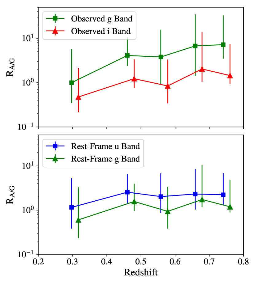
Figure 14: The AGN-to-galaxy flux ratio ($R_{\text{A/G}}$). Each redshift bin has the same number of quasars. The points and the error bars show the median values and the ranges where $68\%$ of the objects are included. The redshifts are shifted slightly to make the error bars of different lines distinguishable. Upper Panel: $R_{\text{A/G}}$ in the $observed$ $g$ and $i$ bands. At $0.2<z<0.8$, $R_{\text{A/G}}$ increases with redshift. Lower Panel: $R_{\text{A/G}}$ in the rest-frame $u$ and $g$ bands. They show little evolution with redshift.

We calculate the rest-frame $u$- and $g$-band absolute magnitudes of the quasar host galaxies based on the host galaxy spectra obtained in our spectroscopic analysis. The median $u-g$ color of the sample is $0.68$ and the standard deviation is $0.40$. Figure 13 shows the color-magnitude diagram (CMD) of these host galaxies. The crosses represent the 8 galaxies with $R^{i}_{\text{gal}}<0.2$, and the dots represent the galaxies with $R^{i}_{\text{gal}}>0.2$. In this figure we also plot the distribution of $0.2<z<0.8$ galaxies from the COSMOS/UltraVISTA $K$-selected galaxy catalog (Muzzin et al., 2013). Compared to these normal galaxies, our quasar host galaxies occupy a different region in the CMD: the host galaxies are significantly more luminous. On the other hand, their global $u-g$ colors are similar to those of star forming galaxies (i.e., galaxies located in the “blue cloud”). All the above suggests that the quasar host galaxies in our sample are mostly luminous star-forming galaxies, which is in consistent with positive AGN feedback. The blue end of the $u-g$ colors are dominated by several objects at $R^{i}_{\text{gal}}<0.2$. As we discussed earlier, these extreme colors are likely caused by the bias and large uncertainties from the imaging decomposition and spectroscopic analysis. Besides those with $R^{i}_{\text{gal}}<0.2$, there are still some objects which are extremely blue $(u-g\sim-0.2)$, yet they are consistent with the “blue cloud” in $\sim 2\sigma$ level.

Figure 14 shows the AGN-to-galaxy flux ratio ($R_{\text{A/G}}$) as the function of redshift. We divide the quasar sample into five redshift bins, with each bin having the same number of quasars. From $z\sim 0.3$ to $\sim 0.7$, the median $R_{\text{A/G}}$ values increase from $\sim 1$ to $\sim 7$ in the observed $g$ band, and from $\sim 0.5$ to $\sim 1$ in the observed $i$ band. The lower panel of the figure shows $R_{\text{A/G}}$ in the rest-frame $u$ and $g$ bands. In the $u$ band, $R_{\text{A/G}}=2.2^{+4.7}_{-0.8}$, and $R_{\text{A/G}}=1.2^{+3.2}_{-0.3}$ in the $g$ band. As expected, $R_{\text{A/G}}$ is larger in the $u$ band. The $R_{\text{A/G}}$ values also suggest that host galaxies are significant in these quasars. There is no obvious trend of $R_{\text{A/G}}$ with redshift. The redshift-dependence in the observed $g$ and $i$ bands mainly arises from the fact that the two observed bands cover different rest-frame wavelength ranges for quasars at different redshifts.

5.2 $M_{*}-M_{\text{BH}}$ Relation

We calculate the stellar masses of the quasar host galaxies using the stellar mass-to-light ratio from Bell et al. (2003):

$$\text{log}(M_{*}/L_{g})=-0.221+0.485\times(u-g),$$ (5)

where $M_{*}$ and $L_{g}$ are in the solar units.

The black hole mass of the quasars are adopted from Shen et al. (in preparation), who use the luminosity at 5100Å $(L_{\text{5100}})$ and the line width of H$\beta$, based on the empirical relation by Vestergaard & Peterson (2006):

$$\begin{split}\text{log}(\frac{M_{\text{BH}}}{M_{\odot}})=a+b~{}\text{log}(\frac{L}{10^{44}\text{ erg s}^{-1}})+c~{}\text{log}(\frac{\text{FWHM}}{\text{km s}^{-1}}),\end{split}$$ (6)

where $a=0.91,b=0.50$, and $c=2$ when using the broad H$\beta$ line and the AGN luminosity at 5100Å, $L_{\text{5100}}$. Shen et al. (in preparation) does not consider the contribution of galaxy fluxes in $L_{\text{5100}}$, which is corrected in this work according to the decomposed spectra in Section 4.

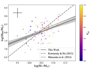
Figure 15: The $M_{*}-M_{\text{BH}}$ relation in the quasar host galaxies. The crosses represent the quasars with $R^{i}_{\text{gal}}<0.2$, and the black dots shows the quasars with $R^{i}_{\text{gal}}>0.2$. The solid line shows the best fit for all quasars, the dashed line shows the $M_{\text{Bulge}}-M_{\text{BH}}$ relation in local galaxies from Kormendy & Ho (2013), and the dot-dashed line represents the relation for $z<0.6$ quasar host galaxies from Matsuoka et al. (2014). The gray area shows the $1\sigma$ error of our fitting result estimated using Bootstrap. This figure suggests that the $M_{*}-M_{\text{BH}}$ of quasar host galaxies are shallower than the $M_{\text{Bulge}}-M_{\text{BH}}$ relation in local galaxies.

Figure 15 shows the $M_{*}-M_{\text{BH}}$ relation of the quasar host galaxies. There is a positive correlation between $M_{*}$ and $M_{\text{BH}}$. We also include the $M_{\text{Bulge}}-M_{\text{BH}}$ relation in local galaxies from Kormendy & Ho (2013) and the relation for $z<0.6$ SDSS quasars from Matsuoka et al. (2014). The stellar masses in our sample and in the Matsuoka et al. (2014) sample include both bulge and disk masses. Figure 15 suggests that the $M_{*}-M_{\text{BH}}$ of quasar host galaxies are shallower than the $M_{\text{Bulge}}-M_{\text{BH}}$ relation in local galaxies.

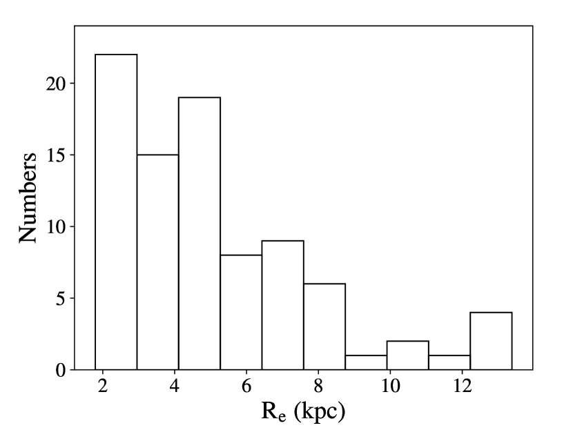
Figure 16: The distribution of the Sérsic parameters of the quasar host galaxies. Upper Panel: The distribution of the half-light radius $R_{e}$. Lower Panel: The distribution of the Sérsic index $n$. In our sample, $n$ spans from $\sim 0.5$ (disk-like) to $\sim 3$ (bulge-like). Most galaxies have $n<2$, indicating that the majority of them are disk-dominated.

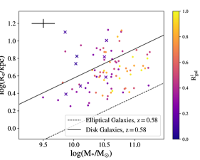
Figure 17: The $M_{*}-R_{e}$ relation of the quasar host galaxies. The crosses represent the quasars with $R^{i}_{\text{gal}}<0.2$, and the black dots shows the quasars with $R^{i}_{\text{gal}}>0.2$. The dashed and solid lines represent the relations for disk and elliptical galaxies at $z=0.58$ (median redshift of our sample), based on Lange et al. (2016) and van der Wel et al. (2014) (see text). The quasar host galaxies in our sample are consistent with late-type galaxies.

5.3 Sérsic Parameters

Figure 16 shows the distribution of the half-light radius $R_{e}$ and Sérsic index $n$ of the host galaxies. The $R_{e}$ values span a wide range from $\sim 2$ to $\sim 13$ kpc, with an average of $\sim 5$ kpc. At $z=0.8$, a half-light radius of 2 kpc corresponds to an angular size of $0\farcs 27$, or $0\farcs 54$ in diameter, which can be marginally resolved by our $i$-band images. The $n$ values span from $\sim 0.5$ to $\sim 3$. Figure 17 shows the relation between $M_{*}$ and $R_{e}$ of the quasar host galaxies. For comparison, we include in Figure 17 the $M_{*}-R_{e}$ relations for disk and elliptical galaxies at $z=0.58$ (the median redshift of our quasar sample). These relations are estimated as follows. We start with the $M_{*}-R_{e}$ relations for local disk and elliptical galaxies at $z<0.06$ from Lange et al. (2016). Galaxies at higher redshift tend to have smaller sizes (e.g., Trujillo et al., 2007; van der Wel et al., 2008, 2014). For example, van der Wel et al. (2014) reported that, at $0<z<3$, the average radius evolves with redshift as $r\propto(1+z)^{-0.75}$ for late-type galaxies and $r\propto(1+z)^{-1.48}$ for early-type galaxies. We take into account this size evolution and find that from $z=0$ to $z=0.58$, the radius of late-type galaxies decreases by $\sim 0.15$ dex and the radius of early-type galaxies decreases by $\sim 0.3$ dex. The relations are plotted in Figure 17. Figure 17 indicates that the $M_{*}-R_{e}$ relation in our quasar host galaxies is consistent with the relation for late-type galaxies. In summary, the distributions of Sérsic index and half-light radius indicate that most of our quasar host galaxies are disk-dominated.

6 Discussion

6.1 Sample Bias

Most SDSS-RM quasars are drawn from the SDSS quasar catalog, with a small fraction ($\sim 5\%$) of quasars discovered by Panoramic Survey Telescope and Rapid Response System (Pan-STARRS) Medium Deep Field survey (Chambers et al., 2016) and the DEEP2 survey (Newman et al., 2013). The final sample is flux-limited ($i<21.7$ mag) and objects with fiber collisions are removed. Since most sources in this sample are SDSS quasars, the completeness of our sample depends strongly on the completeness of the SDSS quasar selection. The completeness of SDSS quasar catalogs has been investigated in many previous papers. For example, Vanden Berk et al. (2005) found that the completeness in SDSS-I is about 89% to its limiting magnitude. Quasars from Pan-STARRS and DEEP2 survey fill in quasars missed by SDSS, and thus these quasars may further increase the sample completeness. In addition, Shen et al. (2015a) found that the number of quasars in this sample is consistent with the number predicted by the quasar luminosity function. All the above indicate that the SDSS-RM quasar sample is fairly complete to its flux limit.

Another bias is introduced by the “Successful Fitting Criteria” in the image decomposition process. The image decomposition is likely to fail for faint host galaxies, which means that we might miss some faint galaxies. Since only 8 out of 103 objects are rejected in this step, and the “success rate” is larger than 80% in all redshift bins, this bias does not affect our results.

6.2 Massive Star Forming Quasar Host Galaxies

Our results are consistent with many previous results based on image decomposition. For example, Matsuoka et al. (2014) studied $z<0.6$ SDSS quasars using the $g$ and $i$ bands (shifted to $z=0.3$; denoted by ${}^{0.3}g$ and ${}^{0.3}i$) to construct the CMDs of quasar host galaxies and normal galaxies. To directly compare to their results, we select a subsample of our quasars at $0.35<z<0.55$ for which ${}^{0.3}g$ and ${}^{0.3}i$ are available from our spectra. This subsample has ${}^{0.3}(g-i)=1.35\pm 0.37$ and absolute magnitude $<^{0.3}M_{i}>=-21.4$, which are similar to the results of Matsuoka et al. (2014).

Xu et al. (2015a) studied $\sim 200$ AGNs at $z<2$ selected from the 24-$\mu$m infrared emission, and measured their SFRs by SED fitting. In a subsequent study, Xu et al. (2015b) concluded that these AGN host galaxies typically have specific SFR consistent with the star-forming main-sequence galaxies. Compared to our work, Xu et al. (2015a) and Xu et al. (2015b) applied a different method to measure the SFRs of galaxies, but reached a similar result.

We also compare our results with Matsuoka et al. (2015), who studied $z<1$ SDSS-RM quasars by decomposing the co-added spectra. They found that the rest-frame $u-r$ colors of the host galaxies are between 0.5 and 2.5 with a median value of $\sim 2.0$. These galaxies are preferencially located in the “green valley”, indicating relatively old stellar populations ($\sim 1.0$ Gyr). The spectral decomposition method in Matsuoka et al. (2015) assumed single stellar populations (SSP). We measure the $u-r$ colors of our host galaxies at $0.2<z<0.5$, where the rest-frame $u$ and $r$ are covered by the BOSS spectra. The $u-r$ colors are roughly between 0.5 and 2.0, with the median value of $\sim 1.4$. For comparison, the blue cloud of inactive galaxies has $u-r\sim 1.2$ in our control sample, thus our quasar host galaxies have similar colors to the blue cloud. The reason for the discrepancy between our results and the Matsuoka et al. (2015) results is not clear.

The low-redshift $(z<1)$ SDSS-RM quasar sample has been analyzed using spectra decomposition by Matsuoka et al. (2015) and by Shen et al. (2015b). So our sample is actually a subset of the sample used by these two studies. We use the same sample to investigate the different results from image and spectral decomposition. Matsuoka et al. (2015) provided the fraction of the host galaxy in the total flux (host fraction) at the rest-frame 4000 Å. For objects that are successfully fitted in both their and our work, we compare the host fraction provided by the two different methods. There is a positive correlation between the two results, but our result is systematically larger. The median of the difference between the host fraction of our work and Matsuoka et al. (2015) is $0.15$. The difference becomes larger with increasing host fraction. Shen et al. (2015b) decomposed the SDSS-RM quasar spectra using principal component analysis method, and provided the host fraction at the rest-frame 5100 Å. We compare their result with our host fraction at the rest-frame 5100 Å and find that our result is larger by $\sim 0.14$. Figure 18 shows the two comparisons. This difference may explain the bluer colors of our host galaxies compared to Matsuoka et al. (2015). In short, our result is consist with most previous studies using image decomposition, but systematically larger than the results from spectral decomposition. This may indicate that the galaxy flux estimated from image decomposition is generally larger than the flux from spectral decomposition.

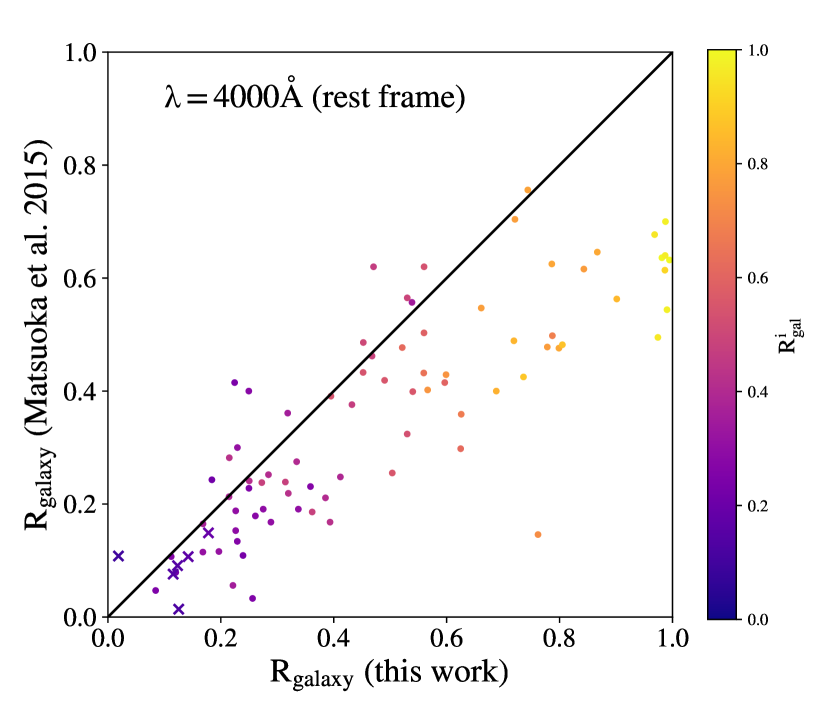
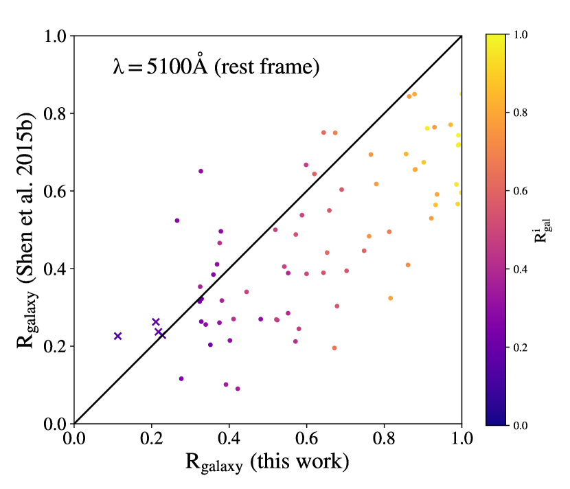
Figure 18: Upper Panel: The fraction of the host galaxy flux in the total flux (host fraction) at the rest-frame 4000Å from this work and Matsuoka et al. (2015). The crosses represent the quasar host galaxies with $R^{i}_{\text{gal}}<0.2$, and the black dots represent the galaxies with $R^{i}_{\text{gal}}>0.2$. There is a positive correlation between our results and Matsuoka et al. (2015), while our results are systematically larger by $\sim 0.15$. The difference increases with the host fraction. Lower Panel: The host fraction at the rest-frame 5100Å from this work and Shen et al. (2015b). Our results are larger by $\sim 0.14$ compared to Shen et al. (2015b). These results indicate that the host galaxy flux provided by image decomposition methods might be systematically larger than the results from spectra decompositions.

6.3 $M_{*}-M_{\text{BH}}$ Relation of Quasar Host Galaxies

Previous studies have reported different results of the $M_{*}-M_{\text{BH}}$ relation for quasar host galaxies. For example, Matsuoka et al. (2014) and Matsuoka et al. (2015) showed a positive correlation between $M_{*}$ and $M_{\text{BH}}$, while Falomo et al. (2014) suggested no correlation.

As shown in Figure 15, there is clearly a positive $M_{*}-M_{\text{BH}}$ correlation in our sample. The best-fit of the $M_{*}-M_{\text{BH}}$ relation is

$$\text{log}(\frac{M_{\text{BH}}}{1.18\times 10^{8}M_{\odot}})=\\ (0.55\pm 0.13)\times\text{log}(\frac{M_{*}}{3.53\times 10^{10}M_{\odot}})+(0.00\pm 0.05).$$ (7)

The errors of the fitting parameters are estimated by Bootstrap. This relation is shallower than the $M_{\text{Bulge}}-M_{\text{BH}}$ relation for local galaxies. The slope of the $M_{\text{BH}}-M_{\text{Bulge}}$ relation for local galaxies is $1.16\pm 0.08$ (Kormendy & Ho, 2013), which is $3.9\sigma$ larger than our result. A shallow relation was also reported in Matsuoka et al. (2014) and Matsuoka et al. (2015). If this shallow relation is physical, it may indicate that the growth of the SMBH mass and the stellar mass in quasars are complex processes and are not synchronized. However, previous studies have suggested that selection biases can influence the observed $M_{*}-M_{\text{BH}}$ relation (e.g., Schulze & Wisotzki, 2011; DeGraf et al., 2015; Shankar et al., 2016). On one hand, the SDSS-RM quasar sample is flux-limited, some low-luminosity (thus low-SMBH-mass) objects might be missed, especially at high redshift. On the other hand, the galaxy sample used to calibrate the local $M_{\text{Bulge}}-M_{\text{BH}}$ relation might also be biased, because a significant fraction of galaxies are selected to have dynamically measured SMBH masses, which requires that the black hole sphere of influence must be resolved (Shankar et al., 2016). The errors of single-epoch SMBH mass measurements may also have significant influence on the observed $M_{*}-M_{\text{BH}}$ relation (e.g., Lauer et al., 2007; Shen & Kelly, 2010). It is difficult to tell whether the discrepancies between quasar host galaxies and local galaxies shown in our results are physical. A detailed discussion about the influence of selection effects on the shallowness of the observed $M_{*}-M_{\text{BH}}$ relation can be found in Shen et al. (2015b).

There are some other sources of systematic errors. First, the stellar masses in our results are calculated using the broad-band flux that is measured according to the co-added SDSS-RM spectra. The diameter of the spectrograph fiber is $2^{\prime\prime}$. Given the wide range of the half-light radius in our sample, we may have missed some flux for some large, low-redshift galaxies, and thus underestimated their stellar masses. Since the measurement of the Sérsic parameters are not accurate, especially for the Sérsic index, it is difficult to correct this systematic error. Second, the stellar masses in our results include both disk and bulge components. The stellar masses should be regarded as upper limits when investigating the $M_{\text{Bulge}}-M_{\text{BH}}$ relation of the quasar hosts. Including disk component in the stellar mass can introduce significant scatters to the $M_{*}-M_{\text{BH}}$ relation. For example, Falomo et al. (2014) performed image decomposition on $z<0.5$ quasars. Different from our approach, they decomposed the host galaxies into bulge and disk components. Their sample shows no correlation between $M_{*}$ and $M_{\text{BH}}$, while there is a significant correlation between $M_{\text{Bulge}}$ and $M_{\text{BH}}$. Our morphology analysis indicates that the host galaxies in our sample have prominent disk components, and may be affected by this systematic error.

6.4 Morphology of Quasar Host Galaxies

Figure 17 shows the $M_{*}-R_{e}$ relation of the quasar host galaxies in our sample. It suggests that the quasar host galaxies are more consistent with late-type galaxies rather than early-type galaxies. The distribution of the Sérsic index also supports this point. As shown in Figure 16, about 70% galaxies have Sérsic index $0.5<n<2$ (disk-like). These results indicate that a significant fraction of quasar host galaxies are disk-dominated. Falomo et al. (2014) reached a similar conclusion for $z<0.6$ quasars.

Morphology of quasar host galaxies can constrain the evolution model of quasars. In major merger models, the quasar host galaxies are expected to be either ellipticals or interacting galaxies, while secular evolution can produce disk-like AGN hosts. Our result suggests that a significant fraction of quasars with $-25<M_{g}<-17$ at $0.2<z<0.8$ are more likely to form by secular evolution. This result is consistent with previous studies (e.g., Cisternas et al., 2011; Villforth et al., 2017), which showed that most low-redshift $(z<1)$ AGN hosts did not exhibit signs of mergers.

7 Summary

We have presented the properties of the host galaxies of 103 $z<0.8$ quasars in the SDSS-RM field. We combined images taken by CFHT/MegaCam, and obtained deep co-added images with $5\sigma$ depth of $\sim 26$ mag in the $i$ band. Each quasar image is decomposed into a PSF and a Sérsic profile, representing the AGN and the galaxy component. A total of 95 out of 103 quasars were successfully decomposed. The systematic error of the galaxy magnitudes is $\sim 0.3$ mag, which is significantly smaller than the errors in most previous ground-based studies. Our main results are:

1. The quasar host galaxies are more massive ($M_{*}\sim 10^{10.5}M_{\odot}$) than inactive galaxies with the same redshifts. They have rest frame $u-g\sim 0.7$ which is similar to star-forming galaxies.

2. The flux from host galaxies is comparable to quasar flux. The typical value of the AGN-to-galaxy flux ratio is $\sim 2.5$ in the rest-frame $u$ band and $\sim 2$ in the rest-frame $g$ band. These ratios show little redshift dependence at $0.2<z<0.8$.

3. The $M_{*}-M_{\text{BH}}$ relation for the quasar host galaxies in our sample is shallower than the local $M_{\text{Bulge}}-M_{\text{BH}}$ relation. This discrepancy may be physical or originate from complex biases.

4. The distribution of the Sérsic indices and the $M_{*}-R_{e}$ relation in our sample indicate that these quasar hosts are dominated by disk-like galaxies.

Our study demonstrates that deep ground-based imaging data with excellent PSF are able to provide reliable estimate of broad-band flux and morphological information for low-redshift quasar host galaxies. In this study, we only have two band data, $g$ and $i$. The large upcoming multi-wavelength sky surveys with great depth and seeing, such as the Hyper-Suprime Cam survey (Aihara et al., 2017) and the Large Synoptic Survey Telescope (LSST Dark Energy Science Collaboration, 2012) will largely expand the quasar sample that is suitable for the image decomposition method and provide more solid conclusions. In addition, future results of the SDSS-RM project will provide more accurate measurements of the BH masses of these quasars, which is crucial for drawing more reliable conclusions about the growth history of SMBH and stellar mass in these quasar host galaxies.

Appendix A Modeling PSF using PSFEx

PSFEx models a PSF using a polynomial function:

$$\text{PSF}(x,y,i,j)=\sum_{m+n\leq N}{A_{m,n}(i,j)x^{m}y^{n}}$$ (A1)

where $x,y$ are the position on the detector, $i,j$ mark the pixel in the PSF model, and $N$ is the degree of the polynomial function. PSFEx provides various choices of the function $A_{m,n}(i,j)$, including pixel-based (i.e., the value of each pixel is a free parameter and can change independently), and some commonly-used analytical functions (e.g., Gaussian, Moffat). When generating the PSF model, PSFEx selects bright, unsaturated, point-like objects based on their flux and half-flux radius, and fits the PSF model in Equation A1 by $\chi^{2}$-minimization. In this study we set $N=3$ and model the PSF in a pixel-based style. Using the $i$ band image of Pointing A as an example, Figure 19 shows the images of $A_{m,n}(i,j)$, and Figure 20 shows the variation of the PSF FWHM across the detector (including all 36 CCD chips). According to Figure 20, that the variation of PSF FWHM across a image is $\lesssim 10\%$.

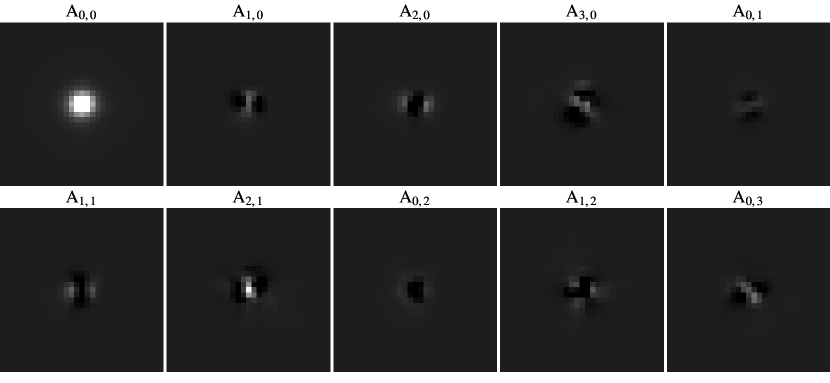
Figure 19: The PSF model of $i$ band image of A pointing generated by PSFEx. See text for the meaning of $A_{m,n}$. The images are shown in logarithmic scale. The $A_{0,0}$ component is the dominate component (the central pixels are saturated to show the details in the other components).

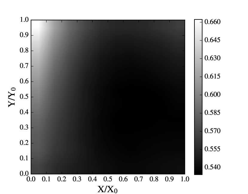
Figure 20: The variation of PSF FWHM across an image. This figure takes the $i$ band image of A pointing as an example. $X_{0}$ and $Y_{0}$ are the size of the image (in pixel). The FWHM of the PSF is expressed in arcsec. The variation of PSF FWHM is $\lesssim 10\%$ in the whole image.

References

- Aihara et al. (2017) Aihara, H., Arimoto, N., Armstrong, R., et al. 2017, arXiv:1704.05858
- Annis et al. (2014) Annis, J., Soares-Santos, M., Strauss, M. A., et al. 2014, ApJ, 794, 120
- Aird et al. (2012) Aird, J., Coil, A. L., Moustakas, J., et al. 2012, ApJ, 746, 90
- Aune et al. (2003) Aune, S., Boulade, O., Charlot, X., et al. 2003, Proc. SPIE, 4841, 513
- Bahcall et al. (1997) Bahcall, J. N., Kirhakos, S., Saxe, D. H., & Schneider, D. P. 1997, ApJ, 479, 642
- Beers et al. (1990) Beers, T. C., Flynn, K., & Gebhardt, K. 1990, AJ, 100, 32
- Bell et al. (2003) Bell, E. F., McIntosh, D. H., Katz, N., & Weinberg, M. D. 2003, ApJS, 149, 289
- Bettoni et al. (2015) Bettoni, D., Falomo, R., Kotilainen, J. K., Karhunen, K., & Uslenghi, M. 2015, MNRAS, 454, 4103
- Bertin & Arnouts (1996) Bertin, E., & Arnouts, S. 1996, A&AS, 117, 393
- Bertin et al. (2002) Bertin, E., Mellier, Y., Radovich, M., et al. 2002, Astronomical Data Analysis Software and Systems XI, 281, 228
- Bertin (2011) Bertin, E. 2011, Astronomical Data Analysis Software and Systems XX, 442, 435
- Brown et al. (2014) Brown, M. J. I., Moustakas, J., Smith, J.-D. T., et al. 2014, ApJS, 212, 18
- Cardelli et al. (1989) Cardelli, J. A., Clayton, G. C., & Mathis, J. S. 1989, ApJ, 345, 245
- Chambers et al. (2016) Chambers, K. C., Magnier, E. A., Metcalfe, N., et al. 2016, arXiv:1612.05560
- Cisternas et al. (2011) Cisternas, M., Jahnke, K., Inskip, K. J., et al. 2011, ApJ, 726, 57
- Cicone et al. (2014) Cicone, C., Maiolino, R., Sturm, E., et al. 2014, A&A, 562, A21
- Croton et al. (2006) Croton, D. J., Springel, V., White, S. D. M., et al. 2006, MNRAS, 365, 11
- DeGraf et al. (2015) DeGraf, C., Di Matteo, T., Treu, T., et al. 2015, MNRAS, 454, 913
- Di Matteo et al. (2005) Di Matteo, T., Springel, V., & Hernquist, L. 2005, Nature, 433, 604
- Eisenstein et al. (2011) Eisenstein, D. J., Weinberg, D. H., Agol, E., et al. 2011, AJ, 142, 72
- Fabian (2012) Fabian, A. C. 2012, ARA&A, 50, 455
- Falomo et al. (2014) Falomo, R., Bettoni, D., Karhunen, K., Kotilainen, J. K., & Uslenghi, M. 2014, MNRAS, 440, 476
- Georgakakis et al. (2008) Georgakakis, A., Nandra, K., Yan, R., et al. 2008, MNRAS, 385, 2049
- Greene & Ho (2005) Greene, J. E., & Ho, L. C. 2005, ApJ, 630, 122
- Gunn et al. (2006) Gunn, J. E., Siegmund, W. A., Mannery, E. J., et al. 2006, AJ, 131, 2332
- Hickox et al. (2009) Hickox, R. C., Jones, C., Forman, W. R., et al. 2009, ApJ, 696, 891
- Hopkins et al. (2006) Hopkins, P. F., Hernquist, L., Cox, T. J., et al. 2006, ApJS, 163, 1
- Jahnke et al. (2004) Jahnke, K., Sánchez, S. F., Wisotzki, L., et al. 2004, ApJ, 614, 568
- Jiang et al. (2014) Jiang, L., Fan, X., Bian, F., et al. 2014, ApJS, 213, 12
- Kauffmann et al. (2003) Kauffmann, G., Heckman, T. M., Tremonti, C., et al. 2003, MNRAS, 346, 1055
- Kim et al. (2008) Kim, M., Ho, L. C., Peng, C. Y., et al. 2008, ApJ, 687, 767-827
- King & Pounds (2015) King, A., & Pounds, K. 2015, ARA&A, 53, 115
- Kirhakos et al. (1999) Kirhakos, S., Bahcall, J. N., Schneider, D. P., & Kristian, J. 1999, ApJ, 520, 67
- Kormendy & Ho (2013) Kormendy, J., & Ho, L. C. 2013, ARA&A, 51, 511
- Lange et al. (2016) Lange, R., Moffett, A. J., Driver, S. P., et al. 2016, MNRAS, 462, 1470
- Lauer et al. (2007) Lauer, T. R., Tremaine, S., Richstone, D., & Faber, S. M. 2007, ApJ, 670, 249
- LSST Dark Energy Science Collaboration (2012) LSST Dark Energy Science Collaboration 2012, arXiv:1211.0310
- Matsuoka et al. (2014) Matsuoka, Y., Strauss, M. A., Price, T. N., III, & DiDonato, M. S. 2014, ApJ, 780, 162
- Matsuoka et al. (2015) Matsuoka, Y., Strauss, M. A., Shen, Y., et al. 2015, ApJ, 811, 91
- McLure et al. (1999) McLure, R. J., Kukula, M. J., Dunlop, J. S., et al. 1999, MNRAS, 308, 377
- Muzzin et al. (2013) Muzzin, A., Marchesini, D., Stefanon, M., et al. 2013, ApJS, 206, 8
- Nandra et al. (2007) Nandra, K., Georgakakis, A., Willmer, C. N. A., et al. 2007, ApJ, 660, L11
- Newman et al. (2013) Newman, J. A., Cooper, M. C., Davis, M., et al. 2013, ApJS, 208, 5
- Oke & Gunn (1983) Oke, J. B., & Gunn, J. E. 1983, ApJ, 266, 713
- Pâris et al. (2017) Pâris, I., Petitjean, P., Ross, N. P., et al. 2017, A&A, 597, A79
- Salomé et al. (2015) Salomé, Q., Salomé, P., & Combes, F. 2015, A&A, 574, A34
- Schlegel et al. (1998) Schlegel, D. J., Finkbeiner, D. P., & Davis, M. 1998, ApJ, 500, 525
- Schulze & Wisotzki (2011) Schulze, A., & Wisotzki, L. 2011, A&A, 535, A87
- Sersic (1968) Sersic, J. L. 1968, Cordoba, Argentina: Observatorio Astronomico
- Shankar et al. (2016) Shankar, F., Bernardi, M., Sheth, R. K., et al. 2016, MNRAS, 460, 3119
- Shen & Kelly (2010) Shen, Y., & Kelly, B. C. 2010, ApJ, 713, 41
- Shen et al. (2015a) Shen, Y., Brandt, W. N., Dawson, K. S., et al. 2015, ApJS, 216, 4
- Shen et al. (2015b) Shen, Y., Greene, J. E., Ho, L. C., et al. 2015, ApJ, 805, 96
- Silverman et al. (2008) Silverman, J. D., Green, P. J., Barkhouse, W. A., et al. 2008, ApJ, 679, 118-139
- Smee et al. (2013) Smee, S. A., Gunn, J. E., Uomoto, A., et al. 2013, AJ, 146, 32
- Spacek et al. (2016) Spacek, A., Scannapieco, E., Cohen, S., Joshi, B., & Mauskopf, P. 2016, ApJ, 819, 128
- Springel et al. (2005) Springel, V., Di Matteo, T., & Hernquist, L. 2005, MNRAS, 361, 776
- Trujillo et al. (2007) Trujillo, I., Conselice, C. J., Bundy, K., et al. 2007, MNRAS, 382, 109
- Trump et al. (2013) Trump, J. R., Hsu, A. D., Fang, J. J., et al. 2013, ApJ, 763, 133
- Tsuzuki et al. (2006) Tsuzuki, Y., Kawara, K., Yoshii, Y., et al. 2006, ApJ, 650, 57
- van der Wel et al. (2008) van der Wel, A., Holden, B. P., Zirm, A. W., et al. 2008, ApJ, 688, 48-58
- van der Wel et al. (2014) van der Wel, A., Franx, M., van Dokkum, P. G., et al. 2014, ApJ, 788, 28
- van Dokkum (2001) van Dokkum, P. G. 2001, PASP, 113, 1420
- Vanden Berk et al. (2005) Vanden Berk, D. E., Schneider, D. P., Richards, G. T., et al. 2005, AJ, 129, 2047
- Véron-Cetty et al. (2004) Véron-Cetty, M.-P., Joly, M., & Véron, P. 2004, A&A, 417, 515
- Vestergaard & Peterson (2006) Vestergaard, M., & Peterson, B. M. 2006, ApJ, 641, 689
- Villforth et al. (2017) Villforth, C., Hamilton, T., Pawlik, M. M., et al. 2017, MNRAS, 466, 812
- Xu et al. (2015a) Xu, L., Rieke, G. H., Egami, E., et al. 2015, ApJS, 219, 18
- Xu et al. (2015b) Xu, L., Rieke, G. H., Egami, E., et al. 2015, ApJ, 808, 159
- York et al. (2000) York, D. G., Adelman, J., Anderson, J. E., Jr., et al. 2000, AJ, 120, 1579
- Zakamska et al. (2005) Zakamska, N. L., Schmidt, G. D., Smith, P. S., et al. 2005, AJ, 129, 1212
- Zinn et al. (2013) Zinn, P.-C., Middelberg, E., Norris, R. P., & Dettmar, R.-J. 2013, ApJ, 774, 66