Anisotropic Error Estimates of The Linear Nonconforming Virtual Element Methods

Abstract

A refined a priori error analysis of the lowest order (linear) nonconforming virtual element method (VEM) for approximating a model Poisson problem is developed in both two and three dimensions. A set of new geometric assumptions is proposed for the shape regularity of polytopal meshes. A new error equation for the lowest order (linear) nonconforming VEM is derived for any choice of stabilization, and a new stabilization using a projection on an extended element patch is introduced for the error analysis on anisotropic elements.

65N12, 65N15, 65N30, 46E35

1 Introduction

In this paper, we develop a modified nonconforming virtual element method (VEM), together with a new way to perform the a priori error analysis for a model Poisson equation. The new analysis incorporates several new geometry assumptions on polytopal partitions in both two and three dimensions.

To approximate multiphysics problems involving complex geometrical features using finite element method (FEM) in 2-D and 3-D, how to encode these geometric information into the discretization is a challenge. To a specific problem’s interest, common practices include either to generate a body/interface-fitted mesh by cutting a shape-regular background mesh, or to build cut-aware approximation spaces/variational forms (stencils) on the unfitted background mesh. Some notable methods utilizing the latter idea include eXtended FEM (e.g., see [28, 37]), fictitious domain FEM [30], cut FEM [17], and immersed FEM [32].

One resolution combining the advantages of both approaches in 3-D was proposed in [21] by using polyhedral meshes rather than the tetrahedral ones. It avoids manually tweaking problematic tetrahedra like slivers with four vertices nearly coplanar, which is usually an unavoidable problem in generating body-fitted mesh from a background mesh, especially when the mesh is fine.

Since arbitrary-shaped polygons or polyhedra are now introduced into the partition, it requires that the underlying finite element methods can handle these kinds of general meshes. There are several classes of modifications of classical numerical methods to work on the polytopal meshes including mimetic finite difference (MFD) [15, 9], generalized barycentric coordinates [29], compatible discrete operator scheme [13], composite/agglomerated discontinuous Galerkin finite element methods (DGFEM) [2], hybridizable discontinuous Galerkin (HDG) methods [20, 23], hybrid high-order (HHO) methods [27, 26], weak Galerkin (WG) methods [38, 34], discontinuous Petrov-Galerkin (PolyDPG) methods [3], etc. Among them, the virtual element method (VEM) introduced in [5] proposed a universal framework for constructing approximation spaces and proving optimal order convergence on polytopal elements. Until now VEMs for elliptic problems have been developed with elaborated details (e.g., see [1, 7, 16, 4, 18, 6]).

The nonconforming finite element method for elliptic problems, better known as Crouzeix-Raviart element, was introduced in [24]. It is nonconforming in the sense that the approximation polynomial space is not a subspace of the underlying Sobolev space corresponding to the continuous weak formulation. Its VEM counterpart was constructed in [4]. The degrees of freedom (DoFs) of a nonconforming VEM function on an element $K$ are the natural dual to this function’s values according to a Neumann boundary value problem on $K$, which are induced by the integral by parts. When a locally constructed stabilization term satisfies the patch test, the convergence in broken $H^{1}$-seminorm is obtained through a systematized approach by showing the norm equivalence for the VEM functions between the broken Sobolev norm and the norm induced by the bilinear form [4].

Establishing the norm equivalence above requires geometric constraints on the shape regularity of the mesh. Almost all VEM error analyses to date are performed on star-shaped elements, and the mostly used assumptions are (1) every element $K$ and every face $F\subset\partial K$ are star-shaped with the chunkiness parameter uniformly bounded above; (2) no short edge/small face, i.e., $h_{F}\eqsim h_{K}$ for every face $F\subset\partial K$. In the former condition, the so-called chunkiness parameter of a star-shaped domain $E$ is the ratio of the diameter of $E$ over the radius of the largest inscribed ball with respect to which $E$ is star-shaped, which may become unbounded for anisotropic elements or anisotropic faces in 3-D star-shaped elements.

Recently, some refined VEM error analyses (see [10, 14]) have removed the “no short edge” assumption in the 2-D conforming VEM by introducing a new tangential derivative-type stabilization first proposed in [39]. In the 3-D case [14], the removal of the “no small face” comes at a price in that the convergence constant depends on the log of the ratio of the longest edge and the shortest edge on a face of a polyhedral element, which also appears in the 2-D analysis using the traditional DoF-type stabilization. This factor seems non-removable due to the norm equivalence being used in these approaches, and it excludes anisotropic elements and/or isotropic elements with anisotropic faces with high aspect ratios in 3-D (e.g. see Figure 4). However, in a variety of numerical tests, some of which even use the traditional stabilization that is suboptimal in theory, VEM performs robustly regardless of these seemingly artificial geometric constraints in situations like random-control-points Voronoi meshes, irregular concave meshes, a polygon degenerating to a line, interface/crack-fitted meshes (see [6, 8, 11, 12, 21, 25, 33]). Especially, anisotropic elements and/or elements with anisotropic faces pose no bottlenecks to the convergence of VEM numerically.

In an effort to partially explain the robustness of VEM regarding the shape regularity of the mesh, in [19], an a priori error analysis for the lowest order conforming VEM is conducted based on a mesh dependent norm $\mathopen{|\mkern-2.5mu|\mkern-2.5mu|}\cdot\mathclose{|\mkern-2.5mu|\mkern-2.5mu|}$ induced by the bilinear form, which is weaker than $H^{1}$-seminorm. The main instrument is an error equation similar to the ones used in the error analysis in Discontinuous Galerkin (DG)-type methods, thus bypassing the norm equivalence. In this way, less geometric constraints are required than the error analysis using the norm equivalence. However, results in [19] are restricted to 2-D, and the anisotropic error analysis is restricted to a special class of elements cut from a shape regular mesh. In particular, long edges in an anisotropic element are required to be paired in order to control the interpolation error in different directions. A precise quantitative characterization of such anisotropic meshes, on which the analysis can be applied, is not explicitly given in [19].

In this paper, we follow this approach, and derive an error equation for the lowest order nonconforming VEM. Thanks to the natural definition of DoFs, the nonconforming interpolation defined using DoFs brings no error into the error estimate in the sense that $\mathopen{|\mkern-2.5mu|\mkern-2.5mu|}u-u_{I}\mathclose{|\mkern-2.5mu|\mkern-2.5mu|}=0$, compared with the error estimates of the conforming interpolant being proved using an intricate edge-pairing technique in [19]. As a result, under geometric conditions introduced in [19], the anisotropic error analysis can be extended to the lowest order nonconforming VEM in both two and three dimensions.

The findings in this paper strengthens our opinion: one of the reasons why VEM is immune to badly shaped elements is that the approximation to the gradient of an $H^{1}$-function is handled by the projection of the gradient of a VEM function, not the exact gradient of it. On the other hand, the flexibility of the VEM framework allows us to modify the stabilization in two ways from the one used in [4] tailored for the anisotropic elements: (1) the weight is changed from the size of each face, respectively, to the diameter of an extended element patch; (2) the stabilization stencil enlarges to this extended element patch, and its form remains the same with the original DoF-type integral, in which the penalization computes now the difference of the VEM functions and their projections onto this extended element patch, not the underlying anisotropic element. In this way, the anisotropic elements can be integrated into the analysis naturally using the tools improved from the results in [38, 31], and an optimal order convergence can be proved in this mesh dependent norm $\mathopen{|\mkern-2.5mu|\mkern-2.5mu|}\cdot\mathclose{|\mkern-2.5mu|\mkern-2.5mu|}$. Our stabilization has the same spirit as the so-called ghost penalty method introduced in [Burman:2010penalty] for fictitious domain methods.

When extending the geometric conditions in [19] from 2-D to 3-D in Section 3, some commonly used tools in finite element analysis, including various trace inequalities and Poincaré inequalities, for simplexes are revisited for polyhedron elements. The conditions these inequalities hold serve as a motivation to propose a set of constraints as minimal as possible on the shapes of elements. In this regard, Assumptions B–C are proposed with more local geometric conditions than the star-shaped condition, which in our opinion is a more “global”-oriented condition for a certain element. Moreover, the hourglass condition in Assumption C allows the approximation on “nice” hourglass-shaped elements, which further relaxes a constraint in the conforming case in [19] in which vertices have to be artificially added to make hourglass-shaped elements isotropic.

As mentioned earlier, the way to deal with an anisotropic element is to assume one can embed this element into an isotropic extended element patch in Assumption D. However the current analysis forbids the existence of a cube/square being cut into thin slabs, in which the number of cuts $\to\infty$ when $h\to 0$. From the standpoint of the implementation, the total number of the anisotropic elements cannot make up a significant portion of all elements in practice, as the enlarged stencil for the modified stabilization makes the stiffness matrix denser.

This paper is organized as follows: In Section 2, the linear nonconforming VEM together with our modification are introduced. Section 3 discusses the aforementioned set of new geometric assumptions in 2-D and 3-D. In Section 4, we derive a new error equation and an a priori error bound for the linear nonconforming VEM. Lastly in Section 5, we study how to alter the assembling procedure in the implementation.

For convenience, $x\lesssim y$ and $z\gtrsim w$ are used to represent $x\leq c_{1}y$ and $z\geq c_{2}w$ respectively, and $a\eqsim b$ means $a\lesssim b$ and $a\gtrsim b$. The constants involved are independent of the mesh size $h$. When there exists certain dependence of these relations to certain geometric properties, then such dependence shall be stated explicitly.

2 Nonconforming Virtual Element Methods

In this section we shall introduce the linear nonconforming virtual element space and corresponding discretization of a model Poisson equation. In order to deal with anisotropic elements, we shall propose a new stabilization term.

Let $\Omega$ be a bounded polytopal domain in $\mathbb{R}^{d}$ $(d=2,3)$, consider the model Poisson equation in the weak form with data $f\in L^{2}(\Omega)$: to find $u\in H_{0}^{1}(\Omega)$ such that

(2.1) $$a(u,v):=(\nabla u,\nabla v)=(f,v)\quad\forall v\in H_{0}^{1}(\Omega).$$

Provided with the mesh satisfying the assumptions to be discussed in Section 3, the goal of this subsection is to build the following discretization using a bilinear form $a_{h}(\cdot,\cdot)$ in a VEM approximation space $V_{h}$ on a given mesh $\mathcal{T}_{h}$, which approximates the original bilinear form $a(\cdot,\cdot)$:

(2.2) $$\text{To find }\;u_{h}\in V_{h},\;\text{ such that}\;\;a_{h}(u_{h},v_{h})=\langle f,v_{h}\rangle\quad\forall v_{h}\in V_{h},$$

where $\langle f,v_{h}\rangle\approx(f,v_{h})$.

2.1 Notation

Throughout the paper the standard notation $(\cdot,\cdot)_{D}$ are used to denote the $L^{2}$-inner product on a domain/hyperplane $D$, and the subscript is omitted when $D=\Omega$. For every geometrical object $D$ and for every integer $k\geq 0$, $\mathbb{P}_{k}(D)$ denotes the set of polynomials of degree $\leq k$ on $D$. The average of an $L^{1}$-integrable function or vector field $v$ over $D$, endowed with the usual Lebesgue measure, is denoted by: $\overline{v}^{D}=|D|^{-1}\int_{D}v$, where $|D|=\operatorname{meas}(D)$.

To approximate problem (2.1), firstly $\Omega$ is partitioned into a polytopal mesh $\mathcal{T}_{h}$, each polytopal element is either a simple polygon ($d=2$) or a simple polyhedron ($d=3$). The set of the elements contained in a subset $D\subset\Omega$ is denoted by $\mathcal{T}_{h}(D):=\{K\in\mathcal{T}_{h}:K\subset\bar{D}\}$. $h:=\max\limits_{K\in\mathcal{T}_{h}}h_{K}$ stands for the mesh size, with $h_{D}:=\operatorname{diam}D$ for any bounded geometric object $D$. Denote $\operatorname{conv}(D)$ be the convex hull of $D$. The term “face” $F$ is usually used to refer to the $(d-1)$-flat face of a $d$-dimensional polytope in this partition ($d=2,3$). For $d=2$ case, a face refers to an edge unless being otherwise specifically stated. The set of all the faces in $\mathcal{T}_{h}$ is denoted by $\mathcal{F}_{h}$. The set of the face $F$ on the boundary of an element $K$ is denoted by $\mathcal{F}_{h}(K)$, and $n_{K}:=|\mathcal{F}_{h}(K)|$ is the number of faces on the boundary of $K$. More generally $\mathcal{F}_{h}(D):=\{F\in\mathcal{F}_{h}:F\subset\bar{D}\}$ denotes faces restricted to a bounded domain $D$. With the help from the context, $\bm{n}_{F}$ denotes the outward unit normal vector of face $F$ with respect to the element $K$. An interior face $F\in\mathcal{F}_{h}$ is shared by two elements $K^{\pm}$. For any function $v$, define the jump of $v$ as $[[{v}]]_{\raisebox{-2.0pt}{\scriptsize$F$}}=v^{-}-v^{+}$ on $F$, where $v^{\pm}=\lim\limits_{\epsilon\to 0}v(\bm{x}-\epsilon\bm{n}_{F}^{\pm})$, and $\bm{n}_{F}^{\pm}$ represents the outward unit normal vector respect to $K^{\pm}$. For a boundary face $F\subset\partial\Omega$, $[[{v}]]_{\raisebox{-2.0pt}{\scriptsize$F$}}:=v|_{F}$.

For a bounded Lipschitz domain $D$, $\left\|\cdot\right\|_{0,D}$ denotes the $L^{2}$-norm, and $|\cdot|_{s,D}$ is the $H^{s}(D)$-seminorm. Again when $D=\Omega$ being the whole domain, the subscript $\Omega$ will be omitted.

2.2 Nonconforming VEM spaces

The lowest order, i.e., the linear nonconforming VEM [4], is the main focus of this article. The linear nonconforming VEM has rich enough content to demonstrate anisotropic meshes’ local impact on the a priori error analysis, and yet elegantly simple enough to be understood without many technicalities. Our main goal is to develop the tools for the linear nonconforming VEM to improve the anisotropic error analysis for the VEM.

The lowest order nonconforming virtual element space $V_{h}$, restricted on an element $K$, can be defined as follows [4]:

(2.3) $$V_{h}(K):=\bigl{\{}v\in H^{1}(K):\quad\Delta v=0\text{ in }K,\,\nabla v\cdot\bm{n}\big{|}_{F}\in\mathbb{P}_{0}(F),\forall F\in\mathcal{F}_{h}(K)\bigr{\}}.$$

The degrees of freedom (DoFs) for the local space $V_{h}(K)$ is the average of $v_{h}\in V_{h}(K)$ on every face $F\in\mathcal{F}_{h}(K)$:

(2.4) $$\chi_{F}(v_{h})=\frac{1}{|F|}\int_{F}v_{h}\,\,{\rm d}S.$$

Denote by this set of DoFs by $\mathcal{N}(K)=\{\chi_{F},F\in\mathcal{F}_{h}(K)\}$ with cardinality $|\mathcal{N}(K)|=n_{K}$, then one can easily verify that $(K,V_{h}(K),\mathcal{N}(K))$ forms a finite element triple in the sense of Chapter 2.3 in [22] (see [4]).

The global nonconforming VEM space $V_{h}$ can be then defined as:

(2.5) $$V_{h}=\bigl{\{}v\in L^{2}(\Omega):\;v\big{|}_{K}\in V_{h}(K),\;\forall K\in\mathcal{T}_{h},\;\int_{F}[[{v}]]_{\raisebox{-2.0pt}{\scriptsize$F$}}\,{\rm d}S=0,\;\forall F\in\mathcal{F}_{h}\bigr{\}}.$$

The canonical interpolation $v_{I}\big{|}_{K}\in V_{h}(K)$ in the nonconforming VEM local space of $v\in H^{1}(K)$ is defined using the DoFs:

(2.6) $$\chi_{F}(v)=\chi_{F}(v_{I}),\quad\forall F\in\mathcal{F}_{h}(K),$$

and the canonical interpolation $v_{I}\in V_{h}$ is then defined using the global DoFs:

(2.7) $$\chi_{F}(v)=\chi_{F}(v_{I}),\quad\forall F\in\mathcal{F}_{h}.$$

2.3 Local projections

The shape functions in $V_{h}(K)$ do not have to be formed explicitly in assembling the stiffness matrix. Based on the construction in (2.3), locally on an element $K$, a certain shape function is the solution to a Neumann boundary value problem, the exact pointwise value of which is unknown. Instead, for $u_{h},v_{h}\in V_{h}(K)$, some computable quantities based on the DoFs of $u_{h}$ and $v_{h}$ are used to compute $a_{h}(u_{h},v_{h})$, which approximates the original continuous bilinear form $a(u_{h},v_{h})$. We now explore what quantities can be computed explicitly using DoFs.

First of all, the $L^{2}$-projection $Q_{F}:v\mapsto Q_{F}v\in\mathbb{P}_{0}(F)$ for any $v\in L^{1}(F)$ to piecewise constant space on a face $F$ is defined as:

(2.8) $$\bigl{(}v-Q_{F}v,q\bigr{)}_{F}=0,\quad\forall q\in\mathbb{P}_{0}(F).$$

For a VEM function $v_{h}\in V_{h}(K)$, this projection can be directly derived from the DoFs (2.4), since $Q_{F}(v_{h})=\chi_{F}(v_{h})$ by definition. In contrast, the $L^{2}$-projection $Q_{K}:L^{1}(K)\to\mathbb{P}_{0}(K)$:

(2.9) $$\bigl{(}v-Q_{K}v,q\bigr{)}_{K}=0,\quad\forall q\in\mathbb{P}_{0}(K).$$

is not computable for $v_{h}\in V_{h}(K)$ by using only the DoFs of $v_{h}$.

On an element $K$, we can also compute an elliptic projection to the linear polynomial space: for any $v\in H^{1}(K)$, $\Pi_{K}v\in\mathbb{P}_{1}(K)$ satisfies

(2.10) $$\left(\nabla\Pi_{K}v,\nabla q\right)_{K}=\left(\nabla v,\nabla q\right)_{K},\quad\text{for all }q\in\mathbb{P}_{1}(K).$$

By choosing $q=x_{i},i=1,\ldots,d,$ one can easily verify $\nabla\Pi_{K}v=Q_{K}(\nabla u)$. Namely $\nabla\Pi_{K}v$ is the best constant approximation of $\nabla u$ in $K$.

As $H^{1}$-semi-inner product is used in (2.10), $\Pi_{K}v$ is unique up to a constant. The constant kernel will be eliminated by the following constraint:

(2.11) $$\int_{\partial K}\Pi_{K}v\,{\rm d}S=\int_{\partial K}v\,{\rm d}S=\sum_{F\in\mathcal{F}_{h}(K)}\,\chi_{F}(v)|F|.$$

Using integration by part, and the fact $\Delta q=0$, $\nabla q$ being constant for $q\in\mathbb{P}_{1}(K)$, the right hand side of (2.10) can be written as

(2.12) $$\left(\nabla v,\nabla q\right)_{K}=(v,\nabla q\cdot\bm{n})_{\partial K}=\sum_{F\in\mathcal{F}_{h}(K)}\nabla q\cdot\bm{n}_{F}\,\chi_{F}(v)|F|.$$

Thus for a VEM function $v_{h}\in V_{h}(K)$, $\Pi_{K}v_{h}$ can be computed by the DoFs of $v_{h}$.

The following lemma shows that $\Pi_{K}$ mapping depends only on DoFs. In this regards, the elliptic projection $\Pi_{K}$ works in a more natural way for nonconforming VEM local space, thanks to the choice of DoFs being the natural dual from the integration by parts.

Lemma 2.1.

For $v,w\in H^{1}(K)$, where $K\in\mathcal{T}_{h}$, if for all $F\in\mathcal{F}_{h}(K)$, $\chi_{F}(v)=\chi_{F}(w)$, then $\Pi_{K}v=\Pi_{K}w$.

Proof 2.2.

This is a direct consequence of definition of $\Pi_{K}$ in view of (2.11)-(2.12).

To incorporate the possibility of the anisotropic analysis, we shall define an extended element patch containing $K$

$$\omega_{K}:={\textstyle\bigcup}_{\alpha\in\Lambda}K_{\alpha}$$

where $\Lambda=\Lambda(K)$ is an index set related to $K$ such that $K\subseteq\omega_{K}$, $K_{\alpha}\in\mathcal{T}_{h}$ for all $\alpha\in\Lambda$, and $\omega_{K}$ is isotropic in the sense of Assumption A–B–C that shall be elaborated in Section 3; for example, see Figure 1(a). When $K$ itself is isotropic, $\omega_{K}=K$.

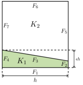
(a)

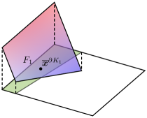
(b)

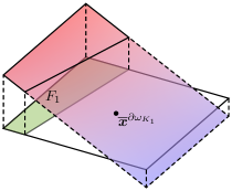
(c)

Figure 1: An illustration of the extended element patch and the elliptic projections on it. As $h\to 0$, $\epsilon\to 0$. (1(a)) $K_{1}$ is anisotropic and $\omega_{K_{1}}=K_{1}\cup K_{2}$ is isotropic. (1(b)) $\Pi_{K_{1}}\phi_{F_{1}}$ in (2.10) has sharp gradient. (1(c)) $\Pi_{\omega_{K_{1}}}\phi_{F_{1}}$ in (2.13) has smoother gradient over $\omega_{K_{1}}$ and is used only in the stabilization term on $\partial K_{1}$, not on $\partial K_{2}$.

We define a discrete $H^{1}$-type projection on $\omega_{K}$ as follows: given a $v_{h}\in V_{h}$

(2.13) $$\left(\nabla\Pi_{\omega_{K}}v_{h},\nabla q\right)_{\omega_{K}}=\sum_{K\in\mathcal{T}_{h}(\omega_{K})}\left(\nabla v_{h},\nabla q\right)_{K},\quad\forall q\in\mathbb{P}_{1}(\omega_{K}).$$

Notice here by the continuity condition in (2.5), it is straightforward to verify that using the integration by parts, for $q\in\mathbb{P}_{1}(\omega_{K})$, on any $F\in\mathcal{F}_{h}(\omega_{K})$, $\nabla q\cdot\bm{n}\big{|}_{F}\in\mathbb{P}_{0}(F)$, and $\Delta q=0$, we have

$$\sum_{K\in\mathcal{T}_{h}(\omega_{K})}\left(\nabla v_{h},\nabla q\right)_{K}=\sum_{K\in\mathcal{T}_{h}(\omega_{K})}\left(v_{h},\nabla q\cdot\bm{n}\right)_{\partial K}$$

$$= \sum_{F\in\mathcal{F}_{h}(\partial\omega_{K})}\left(v_{h},\nabla q\cdot\bm{n}\right)_{F}+\sum_{\begin{subarray}{c}F\in\mathcal{F}_{h}(\omega_{K}),\\ F\not\subset\partial\omega_{K}\end{subarray}}\left([[{v_{h}}]]_{\raisebox{-2.0pt}{\scriptsize$F$}},\nabla q\cdot\bm{n}\right)_{F}=\sum_{F\in\mathcal{F}_{h}(\partial\omega_{K})}\left(v_{h},\nabla q\cdot\bm{n}\right)_{F},$$

of which the right hand side can be evaluated using the DoFs of $v_{h}$ similar to (2.12). When $K\neq\omega_{K}$, the constraint for $\Pi_{\omega_{K}}$, as well as for $\Pi_{K}$ (cf. (2.11)), is chosen as the average on the boundary of $\omega_{K}$: for $v_{h}\in V_{h}$

(2.14) $$\int_{\partial\omega_{K}}\Pi_{K}v_{h}\,{\rm d}S=\int_{\partial\omega_{K}}\Pi_{\omega_{K}}v_{h}\,{\rm d}S=\int_{\partial\omega_{K}}v_{h}\,{\rm d}S,$$

which are both computable using DoFs of $v_{h}$.

In summary, although we do not have access to the pointwise value of $v_{h}\in V_{h}(K)$, we can find its average on each face and a linear polynomial $\Pi_{K}v_{h}$ inside $K$, whose gradient is the best piecewise constant approximation of the element-wise gradient of $v_{h}$. When needed, we can compute another linear polynomial $\Pi_{\omega_{K}}v_{h}$ on an extended patch $\omega_{K}$ (e.g., see Figure 1(c)), the implementation details of which we refer the reader to Section 5.

2.4 Discretization

As the $H^{1}$-projection, $\bigl{(}\nabla\Pi_{K}u_{h},\nabla\Pi_{K}v_{h}\bigr{)}_{K}$ is a good approximation of $(\nabla u_{h},\nabla v_{h})_{K}$. However, $\bigl{(}\nabla\Pi_{K}u_{h},\nabla\Pi_{K}v_{h}\bigr{)}_{K}$ alone will not lead to a stable method as $|\ker(\Pi_{K})|=\dim(V_{h}(K))-\dim\mathbb{P}_{1}(K)\geq 0$ and the equality holds only if $K$ is a simplex. The so-called stabilization term is needed to have a well-posed discretization. The principle of designing a stabilization is two-fold [5]:

1. Consistency. $S_{K}(u,v)$ should vanish when either $u$ or $v$ is in $\mathbb{P}_{1}(K)$. This can be ensured to use the slice operator $(\operatorname{I}-\Pi_{K})$ in the inputs of $S_{K}(\cdot,\cdot)$ beforehand.

2. Stability and continuity. $S_{K}(\cdot,\cdot)$ is chosen so that the following norm equivalence holds

   (2.15) $$a(v,v)\lesssim a_{h}(v,v)\lesssim a(v,v)\quad\forall v\in V_{h}.$$

The original bilinear form used in [4] for problem (2.2) is: for $u_{h},v_{h}\in V_{h}$

$$a_{h}^{\text{orig}}(u_{h},v_{h}):=\sum_{K\in\mathcal{T}_{h}}\bigl{(}\nabla\Pi_{K}u_{h},\nabla\Pi_{K}v_{h}\bigr{)}_{K}+\sum_{K\in\mathcal{T}_{h}}S_{K}^{\text{orig}}\bigl{(}(\mathrm{I}-\Pi_{K})u_{h},(\mathrm{I}-\Pi_{K})v_{h}\bigr{)},$$

where the stabilization term $S_{K}^{\text{orig}}(\cdot,\cdot)$ penalizes the difference between the VEM space and the polynomial projection using DoFs (2.4), while gluing the local spaces together using a weak continuity condition in (2.5): for $u_{h},v_{h}\in V_{h}$

(2.16) $$S_{K}^{\text{orig}}(u_{h},v_{h}):=\sum_{F\in\mathcal{F}_{h}(K)}h_{F}^{d-2}\chi_{F}(u_{h})\chi_{F}(v_{h})$$

The dependence of constants in the norm equivalence (2.15) to the geometry of the element $K$ is, however, not carefully studied in literature. Especially on anisotropic elements, constants hidden in (2.15) could be very large. In 2D and the 3D case when every face $F\in\mathcal{F}_{h}(K)$ is shape-regular, we have the following relation:

(2.17) $$S_{K}^{\text{orig}}(u_{h},v_{h})\eqsim\sum_{F\in\mathcal{F}_{h}(K)}h_{F}^{-1}\bigl{(}Q_{F}u_{h},Q_{F}v_{h}\bigr{)}_{F}.$$

Inspired by this equivalence, we shall use a modified bilinear form: for $u_{h},v_{h}\in V_{h}$

(2.18) $$a_{h}(u_{h},v_{h}):=\sum_{K\in\mathcal{T}_{h}}\Bigl{\{}\bigl{(}\nabla\Pi_{K}u_{h},\nabla\Pi_{K}v_{h}\bigr{)}_{K}+\underbrace{S_{K}\bigl{(}u_{h}-\Pi_{\omega_{K}}u_{h},v_{h}-\Pi_{\omega_{K}}v_{h}\bigr{)}}_{(\mathfrak{s})}\Bigr{\}}.$$

In (2.18), the stabilization on element $K$ is

(2.19) $$(\mathfrak{s}):=\sum_{F\in\mathcal{F}_{h}(K)}h_{\omega_{K}}^{-1}\bigl{(}Q_{F}(u_{h}-\Pi_{\omega_{K}}u_{h}),Q_{F}(v_{h}-\Pi_{\omega_{K}}v_{h})\bigr{)}_{F},$$

which penalizes the difference between a VEM function with its projection $\Pi_{\omega_{K}}$ on the boundary of $K$. To allow faces with small $h_{F}$, the weight is changed to $h_{\omega_{K}}^{-1}$ as well.

Now a nonconforming VEM discretization of (2.1) is: for the bilinear form (2.18), find $u_{h}\in V_{h}$ such that

(2.20) $$a_{h}(u_{h},v_{h})=\displaystyle\sum_{K\in\mathcal{T}_{h}}\bigl{(}f,\Pi_{K}v_{h}\bigr{)}_{K}\quad\forall v_{h}\in V_{h}.$$

In Section 4 we shall derive a general error equation for the difference of the VEM approximation $u_{h}$ to the interpolation $u_{I}$ under the bilinear form induced norm, and present an a priori error bound.

3 Geometric Assumptions and Inequalities

In this section, we explore some constraints to put on the meshes $\mathcal{T}_{h}$ in order that problem (2.20) yields a sensible a priori error estimate.

An element $K\in\mathcal{T}_{h}$ shall be categorized into either “isotropic” or “anisotropic” using some of the following assumptions on the geometry of the mesh. In the following assumptions, the uniformity of the constants is with respect to the mesh size $h\to 0$ in a family of meshes $\{\mathcal{T}_{h}\}$.

3.1 Isotropic elements

Firstly, recall that $n_{K}$ represents the number of faces as well as the number of DoFs in the element $K$. For both isotropic or anisotropic elements, the following assumption shall be fulfilled.

• For $K\in\mathcal{T}_{h}$, the number of faces $n_{K}$ is uniformly bounded.

Secondly, for a simple polygon/polyhedron that is not self-intersecting, a height $l_{F}$, measuring how far from $F$ one can advance to the interior of $K$ in its inward normal direction, determines to what degree of smoothness a function defined on $F$ can be extended into the interior of $K$.

Without loss of generality, the presentation is based on the dimension $d=3$ here, after which the case $d=2$ follows naturally. For a given flat face $F\in\mathcal{F}_{h}(K)$, we choose a local Cartesian coordinate $(\xi,\eta,\tau)$ such that the face $F$ is on the $\tau=0$ plane. For any $x_{F}\in F$, $\bm{x}_{F}=\xi\bm{t}_{F,1}+\eta\bm{t}_{F,2}$, where $\bm{t}_{F,1}$ and $\bm{t}_{F,2}$ are two orthogonal unit vectors that span the hyperplane the face $F$ lies on.

The positive $\tau$-direction is chosen such that it is the inward normal of $F$. Now define:

(3.1) $$\delta_{F}:=\inf\Big{\{}\tau\in\mathbb{R}^{+}:\;K\cap\big{(}F\times(\tau,+\infty)\big{)}=\varnothing\Big{\}}.$$

As $K$ is a simply polyhedral, $\delta_{F}>0$ although it can be very small.

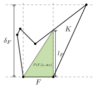
(a)

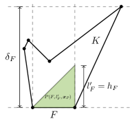
(b)

Figure 2: (2(a)) $l_{F}\geq\gamma_{1}h_{F}$ with $\gamma_{1}>1$. (2(b)) A rescaled $P(F,l_{F}^{\prime},\bm{x}_{P})$ with $l_{F}^{\prime}=h_{F}$.

A pyramid with base $F$, apex $\bm{x}_{P}$, and height $l=\operatorname{dist}(\bm{x}_{P},F)$ is defined as follows:

(3.2) $$P(F,l,\bm{x}_{P}):=\{\bm{x}:\;\bm{x}=(1-t)\bm{x}_{F}+t\bm{x}_{P},t\in(0,1),\bm{x}_{F}\in F\}.$$

Then an inward height $l_{F}$ associated with face $F$ can be defined as follows:

(3.3) $$l_{F}:=\sup\Big{\{}l\in\mathbb{R}^{+}:\exists\,P(F,l,\bm{x}_{P})\subset K\cap\big{(}F\times(0,\delta_{F}]\big{)}\Big{\}}.$$

Here the prism $F\times(0,\delta_{F}]$ is used to ensure the dihedral angles are bounded by $\pi/2$ between $F$ and the side faces of the pyramid $P(F,l_{F},\bm{x}_{P})$.

When $d=2$, as $K$ is non-degenerate (there are no self-intersecting edges) and bounded, $0<\delta_{F}<+\infty$ and $0<l_{F}\leq\delta_{F}$ (see Figure. 2(a) for example). When $d=3$, the existence of such pyramid $P(F,l_{F},\bm{x}_{P})$ is unclear, since $F$ itself can be non-convex. To be able to deal with such case, we impose the following assumption.

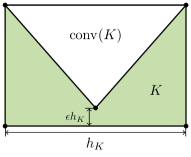
(a)

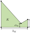
(b)

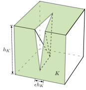
(c)

Figure 3: $\epsilon\to 0$ as $h\to 0$. (3(a)) $K$ has the hourglass shape, and is not an isotropic element in the sense of the geometry assumptions in [19]. Yet this $K$ is isotropic under Assumptions A–B–C. (3(b)) $K$ has a small hourglass-type bump which is ruled out by Assumption C. (3(c)) $K$ with a crack is isotropic, and it has two faces satisfying Assumptions A–B–C in the sense of decompositions.

• (Height condition) There exists a constants $\gamma_{1}>0$, such that $\forall F\in\mathcal{F}_{h}(K)$, it has a partition $F=\bigcup_{\beta\in B_{1}}F_{\beta}$ with $|B_{1}|$ uniformly bounded, such that each $F_{\beta}$ satisfies the height condition $l_{F_{\beta}}\geq\gamma_{1}h_{F}$ and consequently $l_{F}:=\min_{\beta\in B_{1}}l_{F_{\beta}}\geq\gamma_{1}h_{F}$.

In Figure 3(a), the bottom edge satisfies the height condition B only when the decomposition argument is added in the assumption. In Figure 3(c), for the whole front face $F$ without decomposition, no such pyramid in (3.2) exists to yield a sensible (3.3) since there exists points outside $K$ in the line connecting the apex of the pyramid with a point on $F$.

Without loss of generality, one can assume that the constant in Assumption B satisfies $0<\gamma_{1}\leq 1$ when Assumption B is used as a premise of a proposition in later sections. The reason is that, when B holds, one can always rescale the height $l_{F}$ to $l^{\prime}_{F}=\gamma^{\prime}_{1}h_{F}$, for any $0<\gamma^{\prime}_{1}\leq\gamma_{1}$, while the new pyramid $P(F,l^{\prime}_{F},\bm{x}_{P})$ still in $K$. When $\gamma_{1}>1$, we can simply set $\gamma^{\prime}_{1}=1$ to be the new $\gamma_{1}$. See the illustration in Figure 2(b) for an example in 2-D.

Furthermore, in Figure 3(a), it shows a “good” hourglass-shaped element. To avoid small hourglass-type bumps from an element (e.g., see Figure 3(b), the following assumption is imposed.

• (Hourglass condition) $\forall F\in\mathcal{F}_{h}(K)$, it has a partition $F=\bigcup_{\beta\in B_{2}}F_{\beta}$ with $|B_{2}|$ uniformly bounded, such that each $F_{\beta}$ satisfies the hourglass condition: $\forall\beta\in B_{2}$, there exists a convex subset $K_{\beta}\subseteq K$ with $h_{K_{\beta}}\eqsim h_{K}$, such that $P(F_{\beta},l_{F_{\beta}},\bm{x}_{P})\subset K_{\beta}$.

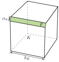
(a)

(b)

(c)

Figure 4: $\epsilon\to 0$ as $h\to 0$. (3(a)) $K$ is a cube without a prismatic slit, the marked face is anisotropic yet the element is isotropic. (3(b)) $K$ itself is anisotropic, all four side faces are anisotropic. (3(c)) $K$ is anisotropic.

Now we say an element $K$ is isotropic if Assumptions A–B–C hold for $K$, with the partitions $\{F_{\beta}\}_{\beta\in B_{1}}=\{F_{\beta}\}_{\beta\in B_{2}}$ for the same face $F$ in Assumptions B–C . Otherwise it is called anisotropic. As we mentioned earlier, isotropy and anisotropy can be formulated for 2-D polygons using the height condition and hourglass condition for edges. A complication in 3-D meshes is that for an isotropic polyhedron, we may have an anisotropic face or a tiny face. In both cases, $|F|\ll h_{K}^{2}$ (see Figure 4 for examples of polyhedral elements). Henceforth, when Assumptions B and/or C are met, we denote $P_{F}:=P(F,l_{F},\bm{x}_{P})$, and whether the decomposition is used or not should be clear from the context.

Lemma 3.1 (Scale of the volume/area for isotropic elements).

If $K$ is isotropic in the sense of Assumptions A–B–C, then $|K|\eqsim h_{K}^{d}$.

Proof 3.2.

Obviously $|K|\lesssim h_{K}^{d}$ by the definition of diameter. It suffices to bound the volume $|K|$ below by $h_{K}^{d}$. We choose the face $F$ with the largest area on $\partial K$, by Assumption A, $|F|\gtrsim|\partial K|$. With slightly abuse of the order of the presentation, by the trace inequality with $v=1$ in Lemma 3.5, we have $|F|=\left\|v\right\|_{0,F}^{2}\lesssim h_{K}^{-1}\left\|v\right\|_{0,K}^{2}=h_{K}^{-1}|K|$. Hence $|K|\gtrsim h_{K}|F|\gtrsim h_{K}|\partial K|$, and the lemma follows from the isoperimetric inequality $|\partial K|\gtrsim|K|^{(d-1)/d}$.

3.2 Anisotropic elements

For anisotropic elements, by definition, there exists faces such that the height condition and/or hourglass condition are violated. The case $l_{F}\ll h_{F}$ can be caused by either the non-convexity of $F$ and $K$, or the chunkiness parameter of $K$ being large.

To be able to use the trace inequalities on a face in an anisotropic element, the following condition on this element $K$ is proposed:

• There exists an isotropic extended element patch $\omega_{K}$ consists of elements in $\mathcal{T}_{h}$ such that

  1. $K\subseteq\omega_{K}$;

  2. $h_{\omega_{K}}\leq\gamma_{2}h$ with a uniform constant $\gamma_{2}>0$;

  3. $\forall F\in\mathcal{F}_{h}(K)$, $F$ satisfies Assumptions B and C toward $\omega_{K}$;

  4. $n_{\omega_{K}}:=\bigl{|}\{K^{\prime}\in\mathcal{T}_{h}(\omega_{K})\}\bigr{|}$ is uniformly bounded above.

By the construction of $\omega_{K}$ and the definition of an isotropic element, the height condition in Assumption B and the hourglass condition in Assumption C are met for every face $F\in\mathcal{F}_{h}(\partial\omega_{K})$. With Assumption D, one can then lift a function defined on a boundary face $F\in\mathcal{F}_{h}({K})$ to the isotropic element $\omega_{K}$.

3.3 Finite overlapping of convex hulls

For polytopal meshes, we impose the following conditions on the convex hull of $K$ for isotropic elements or $\omega_{K}$ for anisotropic elements.

• There exists a uniform constant $\gamma_{3}>0$ such that for each $K\in\mathcal{T}_{h}$

  $$|\{K^{\prime}\in\mathcal{T}_{h}:\operatorname{conv}(\omega_{K^{\prime}})\cap\operatorname{conv}(\omega_{K})\neq\varnothing\}|\leq\gamma_{3}.$$

It can be verified that Assumption E is ensured if for any vertex, there are uniformly bounded number of polytopal elements surrounding this vertex.

3.4 Trace inequalities

When using a trace inequality, one should be extremely careful as the constant depends on the shape of the domain. In this subsection, we shall re-examine several trace inequalities with more explicit analyses on the geometric conditions.

Lemma 3.3 (A trace inequality on a face in a polytopal element).

Suppose for the face $F$, there exists a triangle/pyramid $P_{F}:=P(F,l_{F},\bm{x}_{P})\subset K\cap\big{(}F\times(0,\delta_{F}]\big{)}$ with height $l_{F}$, then the following trace inequality holds:

(3.4) $$\left\|v\right\|_{0,F}\lesssim l_{F}^{-1/2}\left\|v\right\|_{0,P_{F}}+\big{(}h_{F}l_{F}^{-1/2}+l_{F}^{1/2}\big{)}\left\|\nabla v\right\|_{0,P_{F}}.$$

Consequently if furthermore the height condition B is satisfied, it holds that for $P_{F}:=\bigcup_{\beta\in B_{1}}P_{F_{\beta}}$

(3.5) $$\left\|v\right\|_{0,F}\lesssim h_{F}^{-1/2}\left\|v\right\|_{0,P_{F}}+h_{F}^{1/2}\left\|\nabla v\right\|_{0,P_{F}}.$$

Proof 3.4.

We first consider the case $l_{F}\eqsim h_{F}$ when $d=3$. By Lemma A.3 in [38],

(3.6) $$\left\|v\right\|_{0,F}^{2}\lesssim h_{F}^{-1}\left\|v\right\|_{0,P_{\frac{1}{2}}(F,l_{F},\bm{x}_{P})}^{2}+h_{F}\left\|\nabla v\right\|_{0,P_{\frac{1}{2}}(F,l_{F},\bm{x}_{P})}^{2},$$

where $P_{\frac{1}{2}}(F,l_{F},\bm{x}_{P}):=\{\bm{x}:\;\bm{x}=(1-t)\bm{x}_{F}+t\bm{x}_{P},t\in(0,1/2),\bm{x}_{F}\in F\}$. The motivation to truncate the pyramid $P_{F}$ to the prismatoid is that the Jacobian of the mapping from the prismatoid to the prism is bounded.

For a general case, without loss of generality, we assume $l_{F}\leq h_{F}$, since otherwise, one can set $l_{F}=h_{F}$ first and (3.4) still holds by (3.6): we consider the following mapping $(\bm{x}_{F},\tau)\mapsto(\bm{x}_{F},\tau l_{F}/h_{F})$, denote $P:=P_{\frac{1}{2}}(F,l_{F},\bm{x}_{P})$, and let $\nabla_{\bm{x}_{F}}$ be the gradient taken with respect to $(\xi,\eta)$ in $F$’s local coordinate system. Then a straightforward change of variable computation yields:

(3.7) $$\left\|v\right\|_{0,F}^{2}\lesssim l_{F}^{-1}\left\|v\right\|_{0,P}^{2}+h_{F}^{2}l_{F}^{-1}\left\|\nabla_{\bm{x}_{F}}v\right\|_{0,P}^{2}+l_{F}\left\|\partial_{\tau}v\right\|_{0,P}^{2}.$$

When $d=2$, a similar scaling argument can be found in [19, Lemma 6.3] and estimate (3.7) changes to $\left\|v\right\|_{0,e}^{2}\lesssim l_{e}^{-1}\left\|v\right\|_{0,P}^{2}+h_{e}^{2}l_{e}^{-1}\left\|\partial_{x}v\right\|_{0,P}^{2}+l_{e}\left\|\partial_{y}v\right\|_{0,P}^{2}$ for an edge $e$. As a result, (3.4) holds.

When $F$ satisfies Assumption B, $F=\bigcup_{\beta\in B_{1}}F_{\beta}$, each of $F_{\beta}$ satisfies the height condition with disjoint pyramids $P(F_{\beta},l_{F_{\beta}},\bm{x}_{\beta})$. One can rescale all $l_{F_{\beta}}$ to be $l_{F}:=\min\limits_{\beta\in B_{1}}l_{F_{\beta}}$, and $P(F_{\beta},l_{F})\subset P(F_{\beta},l_{F_{\beta}})\subset K\cap\big{(}F_{\beta}\times(0,\delta_{F_{\beta}}]\big{)}$. Thus under Assumption B, $\left\|v\right\|_{0,F}^{2}=\sum_{\beta\in B_{1}}\left\|v\right\|_{0,F_{\beta}}^{2}$ can be estimated by a simple summation of (3.7).

As we mentioned before, even for an isotropic element, it may contain a face $F$ with $h_{F}\ll h_{K}$ and thus the factor $h_{F}^{-1/2}$ in the trace inequality (3.5) may be uncontrollable. Next we shall use the hourglass condition C to replace $h_{F}^{-1/2}$ by a smaller factor $h_{K}^{-1/2}$.

Lemma 3.5 (A trace inequality on a face satisfying the height condition and the hourglass condition).

If a face $F\in\mathcal{F}_{h}(K)$ satisfies the height condition B and the hourglass condition C, then it holds that

(3.8) $$\left\|v\right\|_{0,F}\lesssim h_{K}^{-1/2}\left\|v\right\|_{0,K}+h_{K}^{1/2}\left\|\nabla v\right\|_{0,K}.$$

Proof 3.6.

As the final inequality (3.8) can be trivially generalized from each $F_{\beta}$ to $F=\bigcup_{\beta}F_{\beta}$ using the same argument with the one in Lemma 3.3, we consider only one face $F_{\beta}$ in the decomposition, which shall be denoted by $F$ subsequently in the proof. First Assumption B implies the validity of the trace inequality (3.5). When Assumption C is met, let $K_{F}$ be the convex subset of $K$ containing $P_{F}$. Since (3.8) holds trivially if $h_{F}\eqsim h_{K}$, it suffices to consider the case when $h_{F}\ll h_{K}$. Due to the convexity of $K_{F}$, $\operatorname{conv}(P_{F})\subset K_{F}$, without loss of generality we can assume that $P_{F}$ is convex. Moreover, we recall that the rescaling argument facilitated by Assumption B allows us to set $h_{P_{F}}\eqsim h_{F}$. By $K_{F}\subseteq K$, it suffices to show that:

(3.9) $$h_{F}^{-1}\left\|v\right\|_{0,P_{F}}^{2}\lesssim h_{K}^{-1}\left\|v\right\|_{0,K_{F}}^{2}+h_{K}\left\|\nabla v\right\|_{0,K_{F}}^{2}.$$

By Assumption C, there exists a point $\bm{a}\in K_{F}$, such that $\operatorname{dist}(\bm{a},P_{F})\eqsim h_{K_{F}}\eqsim h_{K}$ and $\operatorname{conv}(\bm{a},P_{F})\subset K_{F}$ (e.g., see Figure 5). Now thanks to the convexity of $P_{F}$, it has the following local polar coordinate representation using $\bm{a}$ as the origin:

(3.10) $$P_{F}=\{\bm{x}=\bm{x}(r,\bm{\omega})=r\bm{\omega}:r_{1}(\bm{\omega})\leq r\leq r_{2}(\bm{\omega}),\bm{\omega}\in A_{F}\subset\mathbb{S}^{d-1},d=2,3\},$$

and $\operatorname{conv}(\bm{a},P_{F})=\{r\bm{\omega}:0\leq r\leq r_{2}(\bm{\omega}),\;\bm{\omega}\in A_{F}\}$.

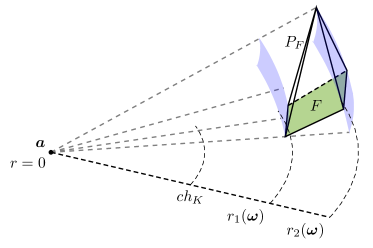
Figure 5: An illustration of $\operatorname{conv}(\bm{a},P_{F})\subset K_{F}$.

For $\bm{x}(r,\bm{\omega})\in P_{F}$, we denote $v(r,\bm{\omega}):=v\big{(}\bm{x}(r,\bm{\omega})\big{)}$. Now for a fixed surface variable $\bm{\omega}$, $|r_{1}(\bm{\omega})-r_{2}(\bm{\omega})|\lesssim h_{F}$, and $r_{i}(\bm{\omega})\eqsim h_{K}$. Moreover, we can choose $\rho$ and constant $c$ bounded away from $0$ independent of $h_{K}$ such that $ch_{K}=\rho<r_{1}(\bm{\omega})$, and thus $|r_{2}(\bm{\omega})-\rho|\gtrsim h_{K}$. The mean value theorem implies that there exists a $\xi\in(\rho,r_{2}(\bm{\omega}))$ such that

(3.11) $$v^{2}(\xi,\bm{\omega})=\frac{1}{|r_{2}(\bm{\omega})-\rho|}\int^{r_{2}(\bm{\omega})}_{\rho}v^{2}(t,\bm{\omega})\,{\rm d}t\lesssim\frac{1}{h_{K}}\int^{r_{2}(\bm{\omega})}_{\rho}v^{2}(t,\bm{\omega})\,{\rm d}t.$$

By the fundamental theorem of calculus, Young’s inequality, and the inequality above, we have

$$v^{2}(r,\bm{\omega}) =v^{2}(\xi,\bm{\omega})+\int^{r}_{\xi}\partial_{t}\big{(}v^{2}(t,\bm{\omega})\big{)}\,{\rm d}t\leq v^{2}(\xi,\bm{\omega})+h_{K}^{-1}\int^{r}_{\xi}v^{2}\,{\rm d}t+h_{K}\int^{r}_{\xi}|\partial_{t}v|^{2}\,{\rm d}t$$

$$\lesssim h_{K}^{-1}\int^{r_{2}(\bm{\omega})}_{\rho}v^{2}\,{\rm d}t+h_{K}\int^{r_{2}(\bm{\omega})}_{\rho}|\partial_{t}v|^{2}\,{\rm d}t,$$

where we note that $\xi$ is not present in the final inequality above, thus this inequality holds for any $\bm{\omega}\in A_{F}$. Integrating above inequality with respect to $r^{d-1}\,{\rm d}r$ and using the fact that $|r_{1}(\bm{\omega})-r_{2}(\bm{\omega})|\leq h_{P_{F}}\eqsim h_{F}$, we have:

$$\int^{r_{2}(\bm{\omega})}_{r_{1}(\bm{\omega})}v^{2}(r,\bm{\omega})r^{d-1}\,{\rm d}r \lesssim\int^{r_{2}(\bm{\omega})}_{r_{1}(\bm{\omega})}\left(h_{K}^{-1}\int^{r_{2}(\bm{\omega})}_{\rho}v^{2}\,{\rm d}t+h_{K}\int^{r_{2}(\bm{\omega})}_{\rho}|\partial_{t}v|^{2}\,{\rm d}t\right)r^{d-1}dr$$

$$\lesssim h_{F}h_{K}^{d-1}\left(h_{K}^{-1}\int^{r_{2}(\bm{\omega})}_{\rho}v^{2}\,{\rm d}t+h_{K}\int^{r_{2}(\bm{\omega})}_{\rho}|\partial_{t}v|^{2}\,{\rm d}t\right):=(\dagger)$$

As $t>\rho=ch_{K}$ in the integrals and $c$ is bounded away from $0$, the factor $h_{K}^{d-1}$ can be moved into the integrals above, thus $(\dagger)$ can be bounded by

$$(\dagger)\lesssim h_{F}\left(h_{K}^{-1}\int^{r_{2}(\bm{\omega})}_{\rho}v^{2}(t,\bm{\omega})t^{d-1}\,{\rm d}t+h_{K}\int^{r_{2}(\bm{\omega})}_{\rho}|\partial_{t}v(t,\bm{\omega})|^{2}t^{d-1}\,{\rm d}t\right).$$

Lastly, $\bm{x}=r\bm{\omega}$ together with $|\bm{\omega}|=1$ implies $|\partial_{t}v(t,\bm{\omega})|\leq|\nabla v|$, integrating both sides of the integral above with respect to surface measure $\,{\rm d}\bm{\omega}$ on $A_{F}$ and rearranging the factors yield:

$$h_{F}^{-1}\left\|v\right\|_{0,P_{F}}^{2}\lesssim h_{K}\left\|v\right\|_{0,\operatorname{conv}(\bm{a},P_{F})}^{2}+h_{K}\left\|\nabla v\right\|_{0,\operatorname{conv}(\bm{a},P_{F})}^{2}.$$

Consequently (3.9) is valid since $\operatorname{conv}(\bm{a},P_{F})\subset K_{F}$, and the lemma follows.

Remark 3.7.

When $K$ is uniformly star-shaped, we can choose the vertex $\bm{a}$ as the center of the largest inscribed ball for all faces $F$. With Assumptions B and C, the vertex $\bm{a}$ could vary for different faces, and thus a more flexible geometry is allowed. See Fig. 3(a) and 3(c) for examples satisfying Assumptions A, B and C but not uniformly star-shaped.

3.5 Poincaré Inequalities

In this subsection, we review Poincaré–Friedrichs inequalities with a constant depending only on the diameter of the domain but not on the shape.

Lemma 3.8 (Poincaré inequality of a linear polynomial on a face).

On any face $F\in\mathcal{F}_{h}(K)$, for a linear polynomial $q\in\mathbb{P}_{1}(F)$, the estimate

$$\left\|q-\overline{q}^{F}\right\|_{0,F}\leq h_{F}\left\|\nabla_{F}q\right\|_{0,F},$$

where $\nabla_{F}$ denotes the surface gradient on $F$.

Proof 3.9.

Here we use the local Cartesian coordinate $\xi\bm{t}_{F,1}+\eta\bm{t}_{F,2}=:\bm{x}\in F$ in defining (3.1), then for $q\in\mathbb{P}_{1}(F)$, $q=\bm{x}\cdot\nabla_{F}q+c$, where $\nabla_{F}q$ is a constant vector. The lemma then follows from the a direct calculation: $q-\overline{q}^{F}=(\bm{x}-\overline{\bm{x}}^{F})\cdot\nabla_{F}q$, and

(3.12) $$\left\|q-\overline{q}^{F}\right\|_{0,F}^{2}\leq\int_{F}|\bm{x}-\overline{\bm{x}}^{F}|^{2}\,|\nabla_{F}q|^{2}\,\,{\rm d}S\leq h_{F}^{2}\left\|\nabla_{F}q\right\|_{0,F}^{2}.$$

Lemma 3.10 (Poincaré inequality of a linear polynomial on the patch).

For a linear polynomial $q\in\mathbb{P}_{1}(\omega_{K})$ such that $\int_{\partial\omega_{K}}q\,\,{\rm d}S=0$, where $\omega_{K}$ satisfies Assumption D, the following estimate holds with a constant independent of the geometries of $K$ or $\omega_{K}$:

$$\left\|q\right\|_{0,K}\leq h_{\omega_{K}}\|\nabla q\|_{0,K}.$$

Proof 3.11.

For $q\in\mathbb{P}_{1}(\omega_{K})$, $q=\bm{x}\cdot\nabla q+c$ with a constant $c$. By the fact that the constraint is imposed on the boundary integral on $\partial\omega_{K}$, similar to the previous lemma, it can be verified that $q=(\bm{x}-\overline{\bm{x}}^{\partial\omega_{K}})\cdot\nabla q$, where

$$\overline{\bm{x}}^{\partial\omega_{K}}=\frac{1}{|\partial\omega_{K}|}\int_{\partial\omega_{K}}\bm{x}\,{\rm d}S=\sum_{F\in\mathcal{F}_{h}(\partial\omega_{K})}\frac{|F|}{|\partial\omega_{K}|}\overline{\bm{x}}^{F},$$

where $\overline{\bm{x}}^{F}\in\operatorname{conv}(F)$, hence $\overline{\bm{x}}^{\partial\omega_{K}}\in\operatorname{conv}(\omega_{K})$. As a result, $|\bm{x}-\overline{\bm{x}}^{\partial\omega_{K}}|\leq h_{\omega_{K}}$, and we have

(3.13) $$\left\|q\right\|_{0,K}^{2}\leq\int_{K}|\bm{x}-\overline{\bm{x}}^{\partial\omega_{K}}|^{2}\,|\nabla q|^{2}\,\,{\rm d}\bm{x}\leq h_{\omega_{K}}^{2}\left\|\nabla q\right\|_{0,K}^{2}.$$

Notice that the constraint is imposed on the boundary of a bigger patch $\omega_{K}$ but the inequality holds on a smaller region $K$. When using this inequality in the a priori error estimate in order to get the optimal rate of convergence, the constant will dependent only on $\gamma_{2}$.

For the approximation property of the polynomial projection, we opt to use the Poincaré inequality on a convex domain, thus to utilize the convex hull of a possible non-convex element.

Lemma 3.12 (Poincaré inequality on the convex hull).

Let $\omega$ be a bounded simple polygon/polyhedron, the following Poincaré inequality holds for any $v\in H^{1}\big{(}\operatorname{conv}(\omega)\big{)}$:

(3.14) $$\left\|v-\overline{v}^{\omega}\right\|_{0,\omega}\leq\frac{h_{\omega}}{\pi}\left\|\nabla v\right\|_{0,\operatorname{conv}(\omega)}.$$

Proof 3.13.

As $\overline{v}^{\omega}$ is the best constant approximation in $L^{2}(\omega)$-norm:

$$\left\|v-\overline{v}^{\omega}\right\|_{0,\omega}\leq\big{\|}v-\overline{v}^{\operatorname{conv}(\omega)}\big{\|}_{0,K}\leq\big{\|}v-\overline{v}^{\operatorname{conv}(\omega)}\big{\|}_{0,\operatorname{conv}(\omega)}\leq\frac{h_{\omega}}{\pi}\|\nabla v\|_{0,\operatorname{conv}(\omega)}.$$

In the last step, the Poincaré inequality on a convex set [35] is used.

We then establish a similar result when the constraint is posed on the boundary integral.

Lemma 3.14 (Poincaré inequality with zero boundary average on isotropic polyhedron).

Let $K$ be a polypotal element satisfying Assumptions A–B, then for any $v\in H^{1}(\operatorname{conv}(K))$, the following Poincaré inequality holds:

(3.15) $$\big{\|}{v-\overline{v}^{\partial K}}\big{\|}_{0,K}\lesssim h_{K}\left\|\nabla v\right\|_{0,\operatorname{conv}(K)}.$$

Proof 3.15.

First triangle inequality implies

(3.16) $$\big{\|}{v-\overline{v}^{\partial K}}\big{\|}_{0,K}\leq\left\|v-\overline{v}^{K}\right\|_{0,K}+\big{\|}{\overline{v}^{K}-\overline{v}^{\partial K}}\big{\|}_{0,K},$$

where the first term can be estimated by Lemma 3.12. Rewriting the second term above and using the Cauchy–Schwarz inequality yield:

(3.17) $$\big{\|}{\overline{v}^{K}-\overline{v}^{\partial K}}\big{\|}_{0,K} =|K|^{1/2}\left|\frac{1}{|\partial K|}\int_{\partial K}(\overline{v}^{K}-v)\,{\rm d}S\right|$$

$$\leq\frac{|K|^{1/2}}{|\partial K|}\sum_{F\in\mathcal{F}_{h}(K)}|F|^{1/2}\left\|v-\overline{v}^{K}\right\|_{0,F}.$$

By the trace inequality in Lemma 3.3

(3.18) $$\left\|v-\overline{v}^{K}\right\|_{0,F}\leq h_{F}^{-1/2}\left\|v-\overline{v}^{K}\right\|_{0,K}+h_{F}^{1/2}\left\|\nabla v\right\|_{0,K}.$$

Applying the Poincaré inequality in Lemma 3.12 on $\left\|v-\overline{v}^{K}\right\|_{0,K}$ and the fact that $h_{F}\leq h_{K}$ yields:

(3.19) $$\big{\|}{\overline{v}^{K}-\overline{v}^{\partial K}}\big{\|}_{0,K}\leq\frac{h_{K}|K|^{1/2}}{|\partial K|}\sum_{F\in\mathcal{F}_{h}(K)}\left(\frac{|F|}{h_{F}}\right)^{1/2}\left\|\nabla v\right\|_{0,\operatorname{conv}(K)}.$$

As $|F|\lesssim h_{F}^{d-1}$ and $|\partial K|=\sum_{F\in\mathcal{F}_{h}(K)}|F|$,

$$\sum_{F\in\mathcal{F}_{h}(K)}\left(\frac{|F|}{h_{F}}\right)^{1/2}\lesssim\sum_{F\in\mathcal{F}_{h}(K)}|F|^{\frac{d-2}{2(d-1)}}\leq n_{K}^{\frac{d}{2(d-1)}}|\partial K|^{\frac{d-2}{2(d-1)}}.$$

Then

$$\frac{|K|^{1/2}}{|\partial K|}\sum_{F\in\mathcal{F}_{h}(K)}\left(\frac{|F|}{h_{F}}\right)^{1/2}\lesssim C(n_{K})\frac{|K|^{1/2}}{|\partial K|^{d/2(d-1)}}\lesssim C(n_{K}),$$

where in the last step, we have used the isoperimetric inequality $|K|\leq C_{d}|\partial K|^{d/(d-1)}$.

4 A Priori Error Analysis

The error analysis will be performed under a mesh dependent norm $\mathopen{|\mkern-2.5mu|\mkern-2.5mu|}\cdot\mathclose{|\mkern-2.5mu|\mkern-2.5mu|}$ induced by $a_{h}(\cdot,\cdot)$, i.e., for $v\in H_{0}^{1}(\Omega)+V_{h}$

(4.1) $$\mathopen{|\mkern-2.5mu|\mkern-2.5mu|}v\mathclose{|\mkern-2.5mu|\mkern-2.5mu|}^{2}:=a_{h}(v,v)=\sum_{K\in\mathcal{T}_{h}}\left(\left\|\nabla\Pi_{K}v\right\|^{2}_{K}+h_{\omega_{K}}^{-1}\sum_{F\in\mathcal{F}_{h}(K)}\left\|Q_{F}(v-\Pi_{\omega_{K}}v)\right\|^{2}_{F}\right).$$

which is weaker than the $H^{1}$-seminorm $|\cdot|_{1}$ upon which the conventional VEM analysis is built. We denote the local norm on $K$ as $\mathopen{|\mkern-2.5mu|\mkern-2.5mu|}\cdot\mathclose{|\mkern-2.5mu|\mkern-2.5mu|}_{K}$. As all projections $\Pi_{K},\Pi_{\omega_{K}},$ and $Q_{F}$ can be computed using only on the DoFs (see (2.12) and (2.13)), it is straightforward to verify that $\mathopen{|\mkern-2.5mu|\mkern-2.5mu|}v-v_{I}\mathclose{|\mkern-2.5mu|\mkern-2.5mu|}=0$ for the interpolant $v_{I}$ defined using DoFs in (2.7).

4.1 A mesh dependent norm

Firstly, the following lemma is needed for proving $\mathopen{|\mkern-2.5mu|\mkern-2.5mu|}\cdot\mathclose{|\mkern-2.5mu|\mkern-2.5mu|}$ is a norm on $V_{h}$ which bounds the projection $\Pi_{\omega_{K}}$ in an extended element measured in the $H^{1}$-seminorm.

Lemma 4.1 (Bound of the projection $\Pi_{\omega_{K}}$ on the patch).

Let $\overline{\omega}=\overline{\cup_{\alpha\in A}K_{\alpha}}$, for $v\in H^{1}(\omega)$, the following estimate holds:

(4.2) $$\left\|\nabla\Pi_{\omega}v\right\|_{0,\omega}^{2}\leq\sum_{\alpha\in A}\left\|\nabla\Pi_{K_{\alpha}}v\right\|_{0,K_{\alpha}}^{2}.$$

Proof 4.2.

By definition (2.10), for any $q\in\mathbb{P}_{1}(\omega)$, $q\big{|}_{K_{\alpha}}\in\mathbb{P}_{1}(K_{\alpha})$, thus by the Cauchy-Schwarz inequality and an $\ell^{2}$–$\ell^{2}$ Hölder inequality, we have

(4.3) $$\left(\nabla\Pi_{\omega}v,\nabla q\right)_{\omega}=\left(\nabla v,\nabla q\right)_{\omega}=\sum_{\alpha\in A}\left(\nabla v,\nabla q\right)_{K_{\alpha}}=\sum_{\alpha\in A}\left(\nabla\Pi_{K_{\alpha}}v,\nabla q\right)_{K_{\alpha}}$$

$$\leq \sum_{\alpha\in A}\left\|\nabla\Pi_{K_{\alpha}}v\right\|_{0,K_{\alpha}}\left\|\nabla q\right\|_{0,K_{\alpha}}\leq\left(\sum_{\alpha\in A}\left\|\nabla\Pi_{K_{\alpha}}v\right\|_{0,K_{\alpha}}^{2}\right)^{1/2}\left\|\nabla q\right\|_{0,\omega}.$$

The lemma then follows from letting $q=\Pi_{\omega}v$.

Lemma 4.3.

$\mathopen{|\mkern-2.5mu|\mkern-2.5mu|}\cdot\mathclose{|\mkern-2.5mu|\mkern-2.5mu|}$ defines a norm on the nonconforming VEM space $V_{h}$.

Proof 4.4.

Since each component of $\mathopen{|\mkern-2.5mu|\mkern-2.5mu|}\cdot\mathclose{|\mkern-2.5mu|\mkern-2.5mu|}$ supports the triangle inequality and is scalable, it suffices to verify that if $\mathopen{|\mkern-2.5mu|\mkern-2.5mu|}v_{h}\mathclose{|\mkern-2.5mu|\mkern-2.5mu|}=0$ for $v_{h}\in V_{h}$, then $v_{h}\equiv 0$. By definition, $a_{h}(v_{h},v_{h})=\mathopen{|\mkern-2.5mu|\mkern-2.5mu|}v_{h}\mathclose{|\mkern-2.5mu|\mkern-2.5mu|}^{2}=0$ implies that

(4.4) $$\nabla\Pi_{K}v_{h}=\bm{0},\;\forall K\in\mathcal{T}_{h};\quad Q_{F}(v_{h}-\Pi_{\omega_{K}}v_{h})=0\text{ on }F,\;\forall F\in\mathcal{F}_{h}(K).$$

Without the loss of generality, we assume that $\omega_{K}$ consists $K$ and $K^{\prime}$ sharing a face, which covers the case of $\omega_{K}=K$ while can be generalized to the case where $\omega_{K}$ contains three or more elements.

Firstly by Lemma 4.1, $\nabla\Pi_{\omega_{K}}v_{h}=\bm{0}$ since $\nabla\Pi_{K}v_{h}=\nabla\Pi_{K^{\prime}}v_{h}=\bm{0}$. Restricting ourselves on $K$, consider the following quantity:

(4.5) $$\;\left\|\nabla v_{h}\right\|_{0,K}^{2}=\bigl{(}\nabla v_{h},\nabla(v_{h}-\Pi_{\omega_{K}}v_{h})\bigr{)}_{K}$$

$$=-\bigl{(}\Delta v_{h},v_{h}-\Pi_{\omega_{K}}v_{h}\bigr{)}_{K}+\left\langle\nabla v_{h}\cdot\bm{n},v_{h}-\Pi_{\omega_{K}}v_{h}\right\rangle_{\partial K}$$

$$=\sum_{F\in\mathcal{F}_{h}(K)}\bigl{(}\nabla v_{h}\cdot\bm{n},Q_{F}(v_{h}-\Pi_{\omega_{K}}v_{h})\bigr{)}_{F}=0.$$

In the last step, $\Delta v_{h}=0$ in $K$ is used. Since $\nabla v_{h}\cdot\bm{n}\in\mathbb{P}_{0}(F)$, the $L^{2}$ projection $Q_{F}$ can be inserted into the pair.

As a result of (4.4), in every $K$, $\nabla v_{h}=\bm{0}$ thus $v_{h}=\text{constant}$. Finally, by the boundary condition and the continuity condition in (2.5), $v_{h}\equiv 0$.

4.2 A priori error estimates on isotropic elements

Next, an error equation is developed for the lowest order nonconforming VEM following [19, 34], and the a priori error analysis on isotropic elements is established.

Lemma 4.5 (An error equation).

Let $u_{h}$ and $u_{I}$ be the solution to problem (2.20) and the canonical interpolation in (2.7) respectively, and let $u_{\pi}$ be any piecewise linear polynomial on $\mathcal{T}_{h}$, for any $v_{h}\in V_{h}$ and stabilization $S_{K}(\cdot,\cdot)$, it holds that

(4.6) $$a_{h}(u_{h}-u_{I},v_{h})= \sum_{K\in\mathcal{T}_{h}}\sum_{F\in\mathcal{F}_{h}(K)}\left\langle\nabla(u-u_{\pi})\cdot\bm{n},Q_{F}v_{h}-\Pi_{K}v_{h}\right\rangle_{F}$$

$$-\sum_{K\in\mathcal{T}_{h}}S_{K}\bigl{(}u_{I}-\Pi_{\omega_{K}}u_{I},v_{h}-\Pi_{\omega_{K}}v_{h}\bigr{)}.$$

Proof 4.6.

Using the VEM discretization problem (2.20), the original PDE $-\Delta u=f$, the definition of the elliptic projection (2.10), and the integration by parts, we have

(4.7) $$\;\quad a_{h}(u_{h}-u_{I},v_{h})$$

$$=\sum_{K\in\mathcal{T}_{h}}\bigl{(}f,\Pi_{K}v_{h}\bigr{)}_{K}-a_{h}(u_{I},v_{h})=\sum_{K\in\mathcal{T}_{h}}\bigl{(}-\Delta u,\Pi_{K}v_{h}\bigr{)}_{K}-a_{h}(u_{I},v_{h})$$

$$=\sum_{K\in\mathcal{T}_{h}}\bigl{(}\nabla\Pi_{K}u,\nabla\Pi_{K}v_{h}\bigr{)}_{K}-\sum_{K\in\mathcal{T}_{h}}\left\langle\nabla u\cdot\bm{n},\Pi_{K}v_{h}\right\rangle_{\partial K}-a_{h}(u_{I},v_{h})$$

$$=\sum_{K\in\mathcal{T}_{h}}\bigl{(}\nabla\Pi_{K}(u-u_{I}),\nabla\Pi_{K}v_{h}\bigr{)}_{K}+\sum_{K\in\mathcal{T}_{h}}\sum_{F\in\mathcal{F}_{h}(K)}\left\langle\nabla u\cdot\bm{n},Q_{F}v_{h}-\Pi_{K}v_{h}\right\rangle_{F}$$

$$\quad-\sum_{K\in\mathcal{T}_{h}}S_{K}\bigl{(}u_{I}-\Pi_{\omega_{K}}u_{I},v_{h}-\Pi_{\omega_{K}}v_{h}\bigr{)}.$$

We note that in the derivation above, on each face $F$, $Q_{F}v_{h}$ which is single-valued on $F$ can be freely inserted into boundary integrals since the inter-element jump of $\nabla u\cdot\bm{n}$ on $F$ vanishes by the assumption that $f\in L^{2}(\Omega)$.

Moreover, since $\chi_{F}(u-u_{I})=0$ for all faces $F$ by (2.6), by Lemma 2.1 we have $\Pi_{K}(u-u_{I})=0$, the first term in (4.7) vanishes. Lastly, using the fact that in the lowest order case, since $u_{\pi}\in\mathbb{P}_{1}(K)$, $\Delta u_{\pi}=0$, the following zero term can be inserted into the boundary integral in (4.7) to get (4.6):

$$\sum_{F\in\partial K}\left\langle\nabla u_{\pi}\cdot\bm{n},Q_{F}v_{h}-\Pi_{K}v_{h}\right\rangle_{F}=\left\langle\nabla u_{\pi}\cdot\bm{n},v_{h}-\Pi_{K}v_{h}\right\rangle_{\partial K}$$

$$= \,\bigl{(}\Delta u_{\pi},v_{h}-\Pi_{K}v_{h}\bigr{)}_{K}+\bigl{(}\nabla u_{\pi},\nabla(v_{h}-\Pi_{K}v_{h})\bigr{)}_{K}=0.$$

Lemma 4.7 (An a priori error estimate on isotropic meshes).

Under the same setting with Lemma 4.5, when the mesh $\mathcal{T}_{h}$ satisfies Assumptions A–B, it holds that

(4.8) $$\mathopen{|\mkern-2.5mu|\mkern-2.5mu|}u_{h}-u_{I}\mathclose{|\mkern-2.5mu|\mkern-2.5mu|}^{2}\lesssim \;\sum_{K\in\mathcal{T}_{h}}\sum_{F\in\mathcal{F}_{h}(K)}h_{K}\left\|\nabla\big{(}u-\Pi_{K}u\big{)}\cdot\bm{n}\right\|_{0,F}^{2}$$

$$\;+ \sum_{K\in\mathcal{T}_{h}}\sum_{F\in\mathcal{F}_{h}(K)}h_{K}^{-1}\left\|u-\Pi_{K}u\right\|_{0,F}^{2}$$

Proof 4.8.

As $\mathcal{T}_{h}$ contains only isotropic elements, $\omega_{K}=K$ for all $K\in\mathcal{T}_{h}$. Let $u_{\pi}=\Pi_{K}u$ and $v_{h}=u_{h}-u_{I}$ in (4.6). Similarly to the proof of Lemma 4.5, definition (2.4) of DoFs with (2.6) implies that $Q_{F}u=Q_{F}u_{I}$, hence $\Pi_{K}u_{I}=\Pi_{K}u$ by Lemma 2.1. As a result, the stabilization term in (4.6) can be estimated as follows:

(4.9) $$\quad S_{K}\bigl{(}u_{I}-\Pi_{K}u_{I},v_{h}-\Pi_{K}v_{h}\bigr{)}$$

$$\leq \sum_{F\in\mathcal{F}_{h}(K)}h_{K}^{-1}\left\|Q_{F}(u_{I}-\Pi_{K}u_{I})\right\|_{0,F}\left\|Q_{F}(v_{h}-\Pi_{K}v_{h})\right\|_{0,F}$$

$$\leq \left(\sum_{F\in\mathcal{F}_{h}(K)}h_{K}^{-1}\left\|Q_{F}(u-\Pi_{K}u)\right\|_{0,F}^{2}\right)^{1/2}\left(\sum_{F\in\mathcal{F}_{h}(K)}h_{K}^{-1}\left\|Q_{F}(v_{h}-\Pi_{K}v_{h})\right\|_{0,F}\right)^{1/2},$$

in which the first term can be estimated by $\left\|Q_{F}(u-\Pi_{K}u)\right\|_{0,F}\leq\left\|u-\Pi_{K}u\right\|_{0,F}$, and the second term is a part of $\mathopen{|\mkern-2.5mu|\mkern-2.5mu|}v_{h}\mathclose{|\mkern-2.5mu|\mkern-2.5mu|}$. For the boundary integral term in (4.6), after using the Cauchy-Schwarz inequality on each face $F$,

(4.10) $$\left\langle\nabla(u-\Pi_{K}u)\cdot\bm{n},Q_{F}v_{h}-\Pi_{K}v_{h}\right\rangle_{F}\leq\left\|\nabla(u-\Pi_{K}u)\cdot\bm{n}\right\|_{0,F}\left\|Q_{F}v_{h}-\Pi_{K}v_{h}\right\|_{0,F},$$

we assign $h_{K}^{1/2}$ to the first term and $h_{K}^{-1/2}$ to the second term in (4.10), and apply the triangle inequality as follows:

(4.11) $$\left\|Q_{F}v_{h}-\Pi_{K}v_{h}\right\|_{0,F}\leq\left\|Q_{F}(v_{h}-\Pi_{K}v_{h})\right\|_{0,F}+\left\|Q_{F}\Pi_{K}v_{h}-\Pi_{K}v_{h}\right\|_{0,F}.$$

Consequently, the first term above, together with the weight $h_{K}^{-1/2}$, is now a part of $\mathopen{|\mkern-2.5mu|\mkern-2.5mu|}v_{h}\mathclose{|\mkern-2.5mu|\mkern-2.5mu|}$. Applying the Poincaré inequality for the linear polynomial $\Pi_{K}v_{h}$ on face $F$ in Lemma 3.8 on the second term above, together with $|F|h_{F}\lesssim|F|l_{F}\leq|K|$ implied by the height condition B, leads to:

(4.12) $$h_{K}^{-1/2}\left\|Q_{F}\Pi_{K}v_{h}-\Pi_{K}v_{h}\right\|_{0,F}\leq h_{F}^{1/2}\left\|\nabla_{F}\Pi_{K}v_{h}\right\|_{0,F}\lesssim\;\left\|\nabla\Pi_{K}v_{h}\right\|_{0,K},$$

which is a part of $\mathopen{|\mkern-2.5mu|\mkern-2.5mu|}v_{h}\mathclose{|\mkern-2.5mu|\mkern-2.5mu|}$. Lastly summing up (4.10) in $\ell^{2}$-sense yields the lemma.

With the a priori error estimate in Lemma 4.7, it suffices to estimate the two terms from estimate (4.8). First we estimate $(u-\Pi_{K}u)$ in the following lemma.

Lemma 4.9 (Error estimate of $\Pi_{K}$ on an isotropic element).

When $K$ satisfies Assumptions A–B–C, for $u\in H^{2}\big{(}\operatorname{conv}(K)\big{)}$ it holds that:

(4.13) $$h_{K}^{-1}\left\|u-\Pi_{K}u\right\|_{0,K}+\left\|\nabla(u-\Pi_{K}u)\right\|_{0,K}\lesssim h_{K}|u|_{2,\operatorname{conv}(K)}.$$

Proof 4.10.

Since $\nabla\Pi_{K}u=\overline{\nabla u}^{K}$, the estimate in the second term follows from the Poincaré inequality in Lemma 3.12. For the first term, by constraint (2.11), applying the Poincaré inequality in Lemma 3.14 and the triangle inequality lead to:

(4.14) $$h_{K}^{-1}\left\|u-\Pi_{K}u\right\|_{0,K}\lesssim\left\|\nabla(u-\Pi_{K}u)\right\|_{0,\operatorname{conv}(K)}$$

$$\leq \;\bigl{\|}\nabla u-\overline{\nabla u}^{\operatorname{conv}(K)}\bigr{\|}_{0,\operatorname{conv}(K)}+\bigl{\|}\overline{\nabla u}^{\operatorname{conv}(K)}-\overline{\nabla u}^{K}\bigr{\|}_{0,\operatorname{conv}(K)}.$$

For the second term above, Cauchy-Schwarz inequality, $|\operatorname{conv}(K)|\lesssim h_{K}^{d}$, and $|K|\eqsim h_{K}^{d}$ in Lemma 3.1 imply that

(4.15) $$\bigl{\|}\overline{\nabla u}^{\operatorname{conv}(K)}-\overline{\nabla u}^{K}\bigr{\|}_{0,\operatorname{conv}(K)}=|\operatorname{conv}(K)|^{1/2}\left|\frac{1}{|K|}\int_{K}\Big{(}{\nabla u}-\overline{\nabla u}^{\operatorname{conv}(K)}\Big{)}\right|$$

$$\leq \;\frac{|\operatorname{conv}(K)|^{1/2}}{|K|^{1/2}}\bigl{\|}\nabla u-\overline{\nabla u}^{\operatorname{conv}(K)}\bigr{\|}_{0,K}\lesssim\bigl{\|}\nabla u-\overline{\nabla u}^{\operatorname{conv}(K)}\bigr{\|}_{0,\operatorname{conv}(K)}.$$

Consequently, the desired estimate follows from applying Lemma 3.12 on $\operatorname{conv}(K)$ and the fact that the diameter of $\operatorname{conv}(K)$ is $h_{K}$.

Lemma 4.11 (Error estimate of the normal derivative of $\Pi_{K}$).

For $K\in\mathcal{T}_{h}$, provided that every $F$ satisfies Assumption B–C, the following error estimate holds on a face $F\in\mathcal{F}_{h}(K)$ for $u\in H^{2}\bigl{(}\operatorname{conv}(K)\bigr{)}$

(4.16) $$h_{K}^{1/2}\left\|\nabla(u-\Pi_{K}u)\cdot\bm{n}\right\|_{0,F}\lesssim h_{K}|u|_{2,\operatorname{conv}(K)}.$$

Proof 4.12.

By Assumption B–C, we apply trace inequality (3.8) toward $K$

(4.17) $$h_{K}^{1/2}\left\|\nabla(u-\Pi_{K}u)\cdot\bm{n}\right\|_{0,F}\lesssim\left\|\nabla(u-\Pi_{K}u)\right\|_{0,K}+h_{K}|{u}|_{2,K}.$$

The lemma then follows from Lemma 4.9.

Lemma 4.13 (Error estimate of $\Pi_{K}$ on a face).

For $K\in\mathcal{T}_{h}$, provided that $K$ satisfies Assumptions A–B–C, the following error estimate holds on a face $F\in\mathcal{F}_{h}(K)$ for $u\in H^{2}\bigl{(}\operatorname{conv}(K)\bigr{)}$:

(4.18) $$h_{K}^{-1/2}\left\|u-\Pi_{K}u\right\|_{0,F}\lesssim h_{K}|u|_{2,\operatorname{conv}(K)}.$$

Proof 4.14.

Since for every $F\in\mathcal{F}_{h}(K)$, $F$ satisfies Assumptions B–C with respect to $K$, by the trace inequality in Lemma 3.5, we have:

(4.19) $$h_{K}^{-1/2}\left\|u-\Pi_{K}u\right\|_{0,F}\lesssim h_{K}^{-1}\left\|u-\Pi_{K}u\right\|_{0,K}+\left\|\nabla(u-\Pi_{K}u)\right\|_{0,K},$$

which yields the desired estimate by Lemma 4.9.

Now the a priori convergence result for the lowest order nonconforming VEM on an isotropic mesh can be summarized as follows.

Theorem 4.15 (Convergence on isotropic meshes).

Assume that the mesh $\mathcal{T}_{h}$ is isotropic in the sense of Assumptions A–B–C–E. When the solution $u$ to (2.1) satisfies $u\in H^{2}(\Omega)$, the following error estimate holds for the solution $u_{h}$ to (2.20):

(4.20) $$\mathopen{|\mkern-2.5mu|\mkern-2.5mu|}u-u_{h}\mathclose{|\mkern-2.5mu|\mkern-2.5mu|}\lesssim h\|u\|_{2,\Omega}.$$

Proof 4.16.

First of all, we apply the Stein’s extension theorem ([36] Theorem 6.5) to $u\in H^{2}(\Omega)$ to get a function $u_{E}\in H^{2}(\mathbb{R}^{d}),u_{E}|_{\Omega}=u|_{\Omega}$, and $\|u_{E}\|_{2,\mathbb{R}^{d}}\leq C(\Omega)\|u\|_{2,\Omega}$. With this extension $u_{E}\in H^{2}\big{(}\operatorname{conv}(K)\big{)}$ for any $K\in\mathcal{T}_{h}$.

Secondly, the estimates from Lemma 4.11 and 4.13 are plugged into Lemma 4.7, and Assumption A ensures that these estimates are summed up bounded times on a fixed element. Meanwhile, Assumption E implies that the integral on the overlap $\operatorname{conv}(K)\cap\operatorname{conv}({K^{\prime}})$ is repeated bounded times for neighboring $K,K^{\prime}\in\mathcal{T}_{h}$. Therefore,

(4.21) $$\mathopen{|\mkern-2.5mu|\mkern-2.5mu|}u_{I}-u_{h}\mathclose{|\mkern-2.5mu|\mkern-2.5mu|}^{2}\lesssim\sum_{K\in\mathcal{T}_{h}}h_{K}^{2}|u_{E}|_{2,\operatorname{conv}(K)}^{2}\lesssim h^{2}|u_{E}|_{2,\operatorname{conv}(\Omega)}^{2}\lesssim h^{2}\|u\|_{2,\Omega}^{2}.$$

As $\mathopen{|\mkern-2.5mu|\mkern-2.5mu|}u-u_{I}\mathclose{|\mkern-2.5mu|\mkern-2.5mu|}=0$ by the construction of $u_{I}$ and (4.1), the theorem follows.

4.3 A priori error estimates on anisotropic elements

In the vanilla error equation (4.6), a boundary term that involves $\Pi_{K}v_{h}$ is present. For an anisotropic element $K$, key estimates including (4.12), (4.17), and (4.19) will become problematic where the Assumptions B–C are violated. Instead, the boundary term will be lifted to its isotropic extended element patch $\omega_{K}$, and thus in next lemma we aim to replace $\Pi_{K}v$ by $\Pi_{\omega_{K}}v$ in the error equation (4.6) taking the anisotropic elements into account.

Lemma 4.17 (Expanded error equation).

Under the same setting with Lemma 4.5, it holds that

(4.22) $$a_{h}(u_{h}-u_{I},v_{h})= \sum_{K\in\mathcal{T}_{h}}\sum_{F\in\mathcal{F}_{h}(K)}\left\langle\nabla(u-u_{\pi})\cdot\bm{n},Q_{F}v_{h}-\Pi_{\omega_{K}}v_{h}\right\rangle_{F}$$

$$-\sum_{K\in\mathcal{T}_{h}}S_{K}\bigl{(}u_{I}-\Pi_{\omega_{K}}u_{I},v_{h}-\Pi_{\omega_{K}}v_{h}\bigr{)}$$

$$+\sum_{K\in\mathcal{T}_{h}}\left(\nabla(u-u_{\pi}),\nabla\bigl{(}\Pi_{\omega_{K}}v_{h}-\Pi_{K}v_{h}\bigr{)}\right)_{K}$$

$$-\sum_{K\in\mathcal{T}_{h}}(f,\Pi_{\omega_{K}}v_{h}-\Pi_{K}v_{h})_{K}.$$

Proof 4.18.

Starting with (4.6), we only need to expand the difference term as follows

$$\sum_{F\in\mathcal{F}_{h}(K)}\left\langle\nabla(u-u_{\pi})\cdot\bm{n},\Pi_{\omega_{K}}v_{h}-\Pi_{K}v_{h}\right\rangle_{F}$$

$$= \,\bigl{(}\Delta(u-u_{\pi}),\Pi_{\omega_{K}}v_{h}-\Pi_{K}v_{h}\bigr{)}_{K}+\bigl{(}\nabla(u-u_{\pi}),\nabla(\Pi_{\omega_{K}}v_{h}-\Pi_{K}v_{h})\bigr{)}_{K}$$

$$= -(f,\Pi_{\omega_{K}}v_{h}-\Pi_{K}v_{h})_{K}+\bigl{(}\nabla(u-u_{\pi}),\nabla(\Pi_{\omega_{K}}v_{h}-\Pi_{K}v_{h})\bigr{)}_{K}.$$

For the last term in (4.22) involving difference in an $L^{2}$-inner product, Poincaré inequalities with appropriate constraints can be applied to change it to the energy norm.

Lemma 4.19 (Difference between projections).

If Assumption D is met for $K$, denote $\mathopen{|\mkern-2.5mu|\mkern-2.5mu|}v_{h}\mathclose{|\mkern-2.5mu|\mkern-2.5mu|}_{\omega_{K}}^{2}:=\sum_{K\in\mathcal{T}_{h}(\omega_{K})}\mathopen{|\mkern-2.5mu|\mkern-2.5mu|}v_{h}\mathclose{|\mkern-2.5mu|\mkern-2.5mu|}_{K}^{2}$, then

(4.23) $$\left\|\Pi_{K}v_{h}-\Pi_{\omega_{K}}v_{h}\right\|_{0,K}\lesssim h_{\omega_{K}}\mathopen{|\mkern-2.5mu|\mkern-2.5mu|}v_{h}\mathclose{|\mkern-2.5mu|\mkern-2.5mu|}_{\omega_{K}}.$$

Proof 4.20.

As we choose the constraint $\int_{\partial\omega_{K}}\Pi_{K}v_{h}=\int_{\partial\omega_{K}}\Pi_{\omega_{K}}v_{h}=\int_{\partial\omega_{K}}v_{h}$, and $\Pi_{K}v_{h}-\Pi_{\omega_{K}}v_{h}$ is a linear polynomial on $K$, the estimate is a direct consequence of Lemma 3.10 and 4.1.

Lemma 4.21 (A priori error estimate using the expanded error equation).

Under the same setting with Lemma 4.5, when $\mathcal{T}_{h}$ satisfies Assumptions A–D, it holds that

(4.24) $$\mathopen{|\mkern-2.5mu|\mkern-2.5mu|}u_{h}-u_{I}\mathclose{|\mkern-2.5mu|\mkern-2.5mu|}^{2}\lesssim \;\sum_{K\in\mathcal{T}_{h}}\sum_{F\in\mathcal{F}_{h}(K)}h_{\omega_{K}}\left\|\nabla\big{(}u-\Pi_{\omega_{K}}u\big{)}\cdot\bm{n}\right\|_{0,F}^{2}$$

$$\;+ \sum_{K\in\mathcal{T}_{h}}\sum_{F\in\mathcal{F}_{h}(K)}h_{\omega_{K}}^{-1}\left\|u-\Pi_{\omega_{K}}u\right\|_{0,F}^{2}$$

$$\;+ \sum_{K\in\mathcal{T}_{h}}\left\|\nabla(u-\Pi_{\omega_{K}}u)\right\|_{0,K}^{2}+\sum_{K\in\mathcal{T}_{h}}h_{\omega_{K}}^{2}\left\|f\right\|_{0,K}^{2}$$

Proof 4.22.

We proceed similarly with the proof of Lemma 4.7 by choosing $v_{h}=u_{h}-u_{I}$, yet letting $u_{\pi}=\Pi_{\omega_{K}}u$ instead in (4.22). The four terms in (4.22) shall be estimated in a backward order. For the fourth term, by the Cauchy-Schwarz inequality and applying Lemma 4.19, we have

(4.25) $$\big{(}f,(\Pi_{K}-\Pi_{\omega_{K}})v_{h}\big{)}_{K}\leq\left\|f\right\|_{0,K}\|(\Pi_{K}-\Pi_{\omega_{K}})v_{h}\|_{K}\lesssim h_{\omega_{K}}\left\|f\right\|_{0,K}\mathopen{|\mkern-2.5mu|\mkern-2.5mu|}v_{h}\mathclose{|\mkern-2.5mu|\mkern-2.5mu|}_{\omega_{K}}.$$

The third term can be estimated in a similar fashion by applying the Cauchy-Schwarz inequality, and applying Lemma 4.1 to get

(4.26) $$\left\|\nabla(\Pi_{\omega_{K}}v_{h}-\Pi_{K}v_{h})\right\|_{0,K}\leq\left\|\nabla\Pi_{\omega_{K}}v_{h}\right\|_{0,\omega_{K}}+\left\|\nabla\Pi_{K}v_{h}\right\|_{0,K}\lesssim\mathopen{|\mkern-2.5mu|\mkern-2.5mu|}v_{h}\mathclose{|\mkern-2.5mu|\mkern-2.5mu|}_{\omega_{K}}.$$

For the second term which is the stabilization, a similar argument with (4.9) in the proof of Lemma 4.7 can be used. By $\mathcal{F}_{h}(\omega_{K})\subset\mathcal{F}_{h}$, Lemma 2.1 implies that $\Pi_{\omega_{K}}u_{I}=\Pi_{\omega_{K}}u$, which leads a similar estimate as the second term in (4.8), and the difference is that $\Pi_{K}$ and $h_{K}$ are replaced in (4.9) by $\Pi_{\omega_{K}}$ and $h_{\omega_{K}}$, respectively.

The first term of (4.22) is treated similarly with (4.10) and (4.11), then since $\omega_{K}$ is isotropic, the rest of the proof, in which $\Pi_{K}$ and $h_{K}$ are replaced by $\Pi_{\omega_{K}}$ and $h_{\omega_{K}}$, proceeds exactly the same with (4.12):

(4.27) $$h_{\omega_{K}}^{-1/2}\left\|Q_{F}\Pi_{\omega_{K}}v_{h}-\Pi_{\omega_{K}}v_{h}\right\|_{0,F}\lesssim h_{F}^{1/2}\left\|\nabla_{F}\Pi_{\omega_{K}}v_{h}\right\|_{0,F}\lesssim\;\left\|\nabla\Pi_{\omega_{K}}v_{h}\right\|_{0,\omega_{K}},$$

and finally the lemma follows from Lemma 4.1.

With the a priori error estimate in Lemma 4.21, it suffices to estimate term by term in (4.24). Since now it involves only the error of the projection on the isotropic extended patch $\omega_{K}$, the estimates in Lemma 4.9, 4.11, and 4.13 can be reused by replacing the $K$ with $\omega_{K}$, both of which are isotropic.

The next theorem summarizes an a priori convergence result that incorporates possible anisotropic elements (cf. Theore 4.15), and we remark that Assumption D includes the scenarios when Assumptions B–C are met as $\omega_{K}=K$.

Theorem 4.23 (Convergence on possible anisotropic meshes).

Assume that the mesh $\mathcal{T}_{h}$ satisfies Assumptions A–D–E. When the solution $u$ to problem (2.1) satisfies $u\in H^{2}(\Omega)$, the following error estimate holds for the solution $u_{h}$ to problem (2.20):

(4.28) $$\mathopen{|\mkern-2.5mu|\mkern-2.5mu|}u-u_{h}\mathclose{|\mkern-2.5mu|\mkern-2.5mu|}\lesssim h\|u\|_{2,\Omega}.$$

Proof 4.24.

We proceed exactly like Theorem 4.15 by extending $u$ to $H^{2}(\mathbb{R}^{d})$ first. The estimate in Lemma 4.9 can be changed straightforwardly on $\omega_{K}$:

(4.29) $$\left\|\nabla(u-\Pi_{\omega_{K}}u)\right\|_{0,\omega_{K}}\lesssim h_{\omega_{K}}|u|_{2,\operatorname{conv}(\omega_{K})}.$$

Since $\omega_{K}$ satisfies Assumptions B–C by Assumption D, the estimates in Lemma 4.13 and 4.11 are changed accordingly on $\omega_{K}$ as well:

(4.30) $$h_{\omega_{K}}^{-1/2}\left\|u-\Pi_{\omega_{K}}u\right\|_{0,F}\lesssim h_{\omega_{K}}|u|_{2,\operatorname{conv}(\omega_{K})},$$

(4.31) and $$h_{\omega_{K}}^{1/2}\left\|\nabla\bigl{(}u-\Pi_{\omega_{K}}u\bigr{)}\cdot\bm{n}\right\|_{0,F}\lesssim h_{\omega_{K}}|u|_{2,\operatorname{conv}(\omega_{K})}.$$

After these estimates are plugged into Lemma 4.21, Assumptions A–E are applied in the same way with Theorem 4.15, except now we consider the integral overlap on patches $\operatorname{conv}(\omega_{K})\cap\operatorname{conv}(\omega_{K^{\prime}})$ for neighboring elements. Upon using the fact that $\left\|f\right\|_{0,K}=\left\|\Delta u\right\|_{0,K}\leq|u|_{2,K}$, we obtain

(4.32) $$\mathopen{|\mkern-2.5mu|\mkern-2.5mu|}u_{I}-u_{h}\mathclose{|\mkern-2.5mu|\mkern-2.5mu|}^{2}\lesssim\sum_{K\in\mathcal{T}_{h}}h_{\omega_{K}}^{2}|u_{E}|_{2,\operatorname{conv}(\omega_{K})}^{2}\lesssim h^{2}|u_{E}|_{2,\operatorname{conv}(\Omega)}^{2}\lesssim h^{2}\|u\|_{2,\Omega}^{2},$$

and the rest of the proof is the same with the one in Theorem 4.15.

5 Concluding remarks and future study

The error analysis in this paper further relaxes and extends to 3-D of the geometry constraints for the linear VEM’s conforming counterpart in [19], and Assumptions B–C can generalized for arbitrary dimension. Since the stabilization is of a weighted $L^{2}$-type, unlike the analysis in [19] bridging the stabilization with a discrete $H^{1/2}$-norm on boundary, the versatility of the VEM framework allows the stabilization in the nonconforming VEM to be more flexible and localizable.

As a result, even for the isotropic case in 3D, the current analysis allows a tiny face and anisotropic face provided that the element is isotropic in the sense of Assumptions B–C, in addition to two alternative shape regularity conditions in Assumptions A–E. In our view, being “isotropic” for an element is a localized property near a face, in that the tangential direction and the normal direction of this face are comparable by the height condition B. Furthermore, the hourglass condition C can be viewed as a localized star-shaped condition for face $F$, where $K_{F}$ can be different for different $F$. The convexity of $K_{F}$ allows that any line connecting a point in $K_{F}$ to a face of $P_{F}$ is entirely in $K_{F}$ (cf. Remark 3.7), which makes $K_{F}$’s role similar to the inscribed ball to which $K$ is uniformly star-shaped in the traditional VEM analysis. Meanwhile the existence of concave faces are allowed in the decomposition sense.

One of the major factors facilitating the new analysis is the introduction of the stabilization on an extended element patch in the discretization (2.18). We remark some of the concerns regarding the implementation using a 2-D example in the following subsection.

5.1 Implementation remarks on the extended patch

When $\mathcal{T}_{h}$ is a body-fitted mesh generated by cutting a shape-regular background grid, $\omega_{K}$, which is only needed for certain anisotropic cut elements $\{K\}$, can be naturally chosen as the patch joining $K$ with one of $K$’s nearest neighbors in the background mesh. Here we shall illustrate using the elements $K_{1},K_{2}\in\mathcal{T}_{h}$ in Figure 1(a), which are cut from a Cartesian mesh in 2-D.

When $\mathcal{T}_{h}$ is not generated from cutting a background shape-regular mesh, the situation is much more complicated, as the search for a possible extended element patch may produce more overhead. To pin down $\omega_{K}$ for an anisotropic $K$, one possible procedure is to estimate the chunkiness parameter of $K$ first: computing $|K|$ and diameter $h_{F}$ of an edge or a face $F\subset\partial K$, if the ratio $h_{F}/|K|^{1/d}$ is bigger than a threshold, then $K$ shall be treated as anisotropic. Starting from an anisotropic element, we can join its immediate neighbor sharing an edge or a face with $K$ to form $\omega_{K}$ and having the minimum chunkiness parameter among all neighbors. Lastly this test is repeated when necessary until $\omega_{K}$ passes the test.

In the implementation, using the data structure for polyhedral elements [21], we can use one array to store all faces and another to story the indices of the polyhedra to which the every face belongs. In this regard, the elements are represented by these two arrays, and the merging of neighboring elements is very efficient; we refer the reader to [21, Section 3.2] for technical details.

5.2 Implementation of the new stabilization

In the element-wise assembling of the matrix corresponding to the bilinear form (2.18), we shall separate the terms of the projected gradient part $\bigl{(}\nabla\Pi_{K}u_{h},\nabla\Pi_{K}v_{h}\bigr{)}_{K}$ and the stabilization part $S_{K}\bigl{(}u_{h}-\Pi_{\omega_{K}}u_{h},v_{h}-\Pi_{\omega_{K}}v_{h}\bigr{)}$. The former remains unchanged from the unmodified formulation. We focus on the implementation of the stabilization term.

For each anisotropic element $K$, assume that we have found an extended patch $\omega_{K}$ which itself is also represented as a polytopal element. Then ${\Pi}_{\omega_{K}}$ can be realized by a matrix $\bm{\Pi}_{\omega_{K}}$ of size $(d+1)\times n_{\omega_{K}}$. The $L^{2}$-projection $Q_{F}$ on $F\in\mathcal{F}_{h}(\partial K)$ applied to a linear polynomial is realized by the DoF matrix $\mathbf{D}$ of size $n_{K}\times(d+1)$. See [7] for detailed formulations of matrices $\bm{\Pi}_{\omega_{K}}$ and $\mathbf{D}$. Denote by $\bar{\mathbf{I}}=(\mathbf{I}\quad\bm{0})_{n_{K}\times n_{\omega_{K}}}$ the extended identity matrix. The stabilization on $K$ can be realized by an $n_{\omega_{K}}\times n_{\omega_{K}}$ local matrix

(5.1) $$h_{\omega_{K}}^{-1}(\bar{\mathbf{I}}-\mathbf{D}\bm{\Pi}_{\omega_{K}})^{\intercal}{\rm diag}(|F_{1}|,\ldots,|F_{n_{K}}|)(\bar{\mathbf{I}}-\mathbf{D}\bm{\Pi}_{\omega_{K}}).$$

Thus the standard assembling procedure looping over all elements can be applied to assemble a global one.

As a comparison, the original stabilization using $\Pi_{K}$ is a matrix of size $n_{K}\times n_{K}$ and in the form $h_{K}^{-1}(\mathbf{I}-\mathbf{D}\bm{\Pi}_{K})^{\intercal}{\rm diag}(|F_{1}|,\ldots,|F_{n_{K}}|)(\mathbf{I}-\mathbf{D}\bm{\Pi}_{K})$. We note that one effect of enlarging the element is that the stabilization matrix (5.1) is denser or equivalently the stencil is larger.

References

- [1] B. Ahmad, A. Alsaedi, F. Brezzi, L. D. Marini, and A. Russo, Equivalent projectors for virtual element methods, Computers & Mathematics with Applications, 66 (2013), pp. 376–391.
- [2] P. F. Antonietti, A. Cangiani, J. Collis, Z. Dong, E. H. Georgoulis, S. Giani, and P. Houston, Review of discontinuous galerkin finite element methods for partial differential equations on complicated domains, in Building Bridges: Connections and Challenges in Modern Approaches to Numerical Partial Differential Equations, Springer, 2016, pp. 281–310.
- [3] A. V. Astaneh, F. Fuentes, J. Mora, and L. Demkowicz, High-order polygonal discontinuous petrov–galerkin (polydpg) methods using ultraweak formulations, Computer Methods in Applied Mechanics and Engineering, 332 (2018), pp. 686–711.
- [4] B. Ayuso de Dios, K. Lipnikov, and G. Manzini, The nonconforming virtual element method, ESAIM: Mathematical Modelling and Numerical Analysis (M2AN), 50 (2016), pp. 879–904.
- [5] L. Beirão da Veiga, F. Brezzi, A. Cangiani, G. Manzini, L. D. Marini, and A. Russo, Basic Principles of Virtual Element Methods, Mathematical Models and Methods in Applied Sciences, 23 (2012), pp. 1–16.
- [6] L. Beirão da Veiga, F. Brezzi, L. Marini, and A. Russo, Virtual element method for general second-order elliptic problems on polygonal meshes, Mathematical Models and Methods in Applied Sciences, 26 (2016), pp. 729–750.
- [7] L. Beirão da Veiga, F. Brezzi, L. D. Marini, and A. Russo, The hitchhiker’s guide to the virtual element method, Mathematical models and methods in applied sciences, 24 (2014), pp. 1541–1573.
- [8] L. Beirão da Veiga, F. Dassi, and A. Russo, High-order virtual element method on polyhedral meshes, Computers & Mathematics with Applications, (2017).
- [9] L. Beirao da Veiga, K. Lipnikov, and G. Manzini, The mimetic finite difference method for elliptic problems, vol. 11, Springer, 2014.
- [10] L. Beirão da Veiga, C. Lovadina, and A. Russo, Stability analysis for the virtual element method, Mathematical Models and Methods in Applied Sciences, 27 (2017), pp. 2557–2594.
- [11] M. F. Benedetto, S. Berrone, S. Pieraccini, and S. Scialò, The virtual element method for discrete fracture network simulations, Computer Methods in Applied Mechanics and Engineering, 280 (2014), pp. 135–156.
- [12] S. Berrone and A. Borio, Orthogonal polynomials in badly shaped polygonal elements for the virtual element method, Finite Elements in Analysis and Design, 129 (2017), pp. 14–31.
- [13] J. Bonelle and A. Ern, Analysis of compatible discrete operator schemes for elliptic problems on polyhedral meshes, ESAIM: Mathematical Modelling and Numerical Analysis, 48 (2014), pp. 553–581.
- [14] S. C. Brenner and L.-Y. Sung, Virtual element methods on meshes with small edges or faces, Mathematical Models and Methods in Applied Sciences, 28 (2018), pp. 1291–1336.
- [15] F. Brezzi, A. Buffa, and K. Lipnikov, Mimetic finite differences for elliptic problems, ESAIM: Mathematical Modelling and Numerical Analysis, 43 (2009), pp. 277–295.
- [16] F. Brezzi, R. S. Falk, and L. D. Marini, Basic principles of mixed virtual element methods, ESAIM: Mathematical Modelling and Numerical Analysis, 48 (2014), pp. 1227–1240.
- [17] E. Burman, S. Claus, P. Hansbo, M. G. Larson, and A. Massing, Cutfem: Discretizing geometry and partial differential equations, International Journal for Numerical Methods in Engineering, 104 (2015), pp. 472–501.
- [18] A. Cangiani, G. Manzini, and O. J. Sutton, Conforming and nonconforming virtual element methods for elliptic problems, IMA Journal of Numerical Analysis, (2016), p. drw036.
- [19] S. Cao and L. Chen, Anisotropic error estimates of the linear virtual element method on polygonal meshes, SIAM Journal on Numerical Analysis, 56 (2018), pp. 2913–2939.
- [20] P. Castillo, B. Cockburn, I. Perugia, and D. Schötzau, An a priori error analysis of the local discontinuous galerkin method for elliptic problems, SIAM Journal on Numerical Analysis, 38 (2000), pp. 1676–1706.
- [21] L. Chen, H. Wei, and M. Wen, An interface-fitted mesh generator and virtual element methods for elliptic interface problems, Journal of Computational Physics, 334 (2017), pp. 327–348.
- [22] P. G. Ciarlet, The Finite Element Method for Elliptic Problems, vol. 4 of Studies in Mathematics and its Applications, North-Holland Publishing Co., Amsterdam-New York-Oxford, 1978.
- [23] B. Cockburn, D. A. Di Pietro, and A. Ern, Bridging the hybrid high-order and hybridizable discontinuous galerkin methods, ESAIM: Mathematical Modelling and Numerical Analysis, 50 (2016), pp. 635–650.
- [24] M. Crouzeix and P.-A. Raviart, Conforming and nonconforming finite element methods for solving the stationary stokes equations i, Revue française d’automatique informatique recherche opérationnelle. Mathématique, 7 (1973), pp. 33–75.
- [25] F. Dassi and L. Mascotto, Exploring high-order three dimensional virtual elements: Bases and stabilizations, Computers & Mathematics with Applications, 75 (2018), pp. 3379 – 3401.
- [26] D. A. Di Pietro and A. Ern, A hybrid high-order locking-free method for linear elasticity on general meshes, Computer Methods in Applied Mechanics and Engineering, 283 (2015), pp. 1–21.
- [27] D. A. Di Pietro, A. Ern, and S. Lemaire, An arbitrary-order and compact-stencil discretization of diffusion on general meshes based on local reconstruction operators, Computational Methods in Applied Mathematics, 14 (2014), pp. 461–472.
- [28] J. Dolbow and T. Belytschko, A finite element method for crack growth without remeshing, Int. J. Numer. Meth. Engng, 46 (1999), pp. 131–150.
- [29] A. Gillette, A. Rand, and C. Bajaj, Error Estimates for Generalized Barycentric Interpolation., Advances in computational mathematics, 37 (2012), pp. 417–439.
- [30] J. Haslinger and Y. Renard, A new fictitious domain approach inspired by the extended finite element method, SIAM Journal on Numerical Analysis, 47 (2009), pp. 1474–1499.
- [31] J. Li, J. M. Melenk, B. Wohlmuth, and J. Zou, Optimal a priori estimates for higher order finite elements for elliptic interface problems, Applied numerical mathematics, 60 (2010), pp. 19–37.
- [32] Z. Li, T. Lin, and X. Wu, New cartesian grid methods for interface problems using the finite element formulation, Numerische Mathematik, 96 (2003), pp. 61–98.
- [33] L. Mascotto, Ill-conditioning in the virtual element method: Stabilizations and bases, Numerical Methods for Partial Differential Equations, 34 (2018), pp. 1258–1281.
- [34] L. Mu, J. Wang, and X. Ye, A weak Galerkin finite element method with polynomial reduction, Journal of Computational and Applied Mathematics, 285 (2015), pp. 45–58.
- [35] L. E. Payne and H. F. Weinberger, An optimal Poincaré inequality for convex domains, Archive for Rational Mechanics and Analysis, 5 (1960), pp. 286–292.
- [36] E. M. Stein, Singular Integrals and Differentiability Properties of Functions, vol. 2, Princeton University Press, 1970.
- [37] N. Sukumar, N. Moës, B. Moran, and T. Belytschko, Extended finite element method for three-dimensional crack modelling, International journal for numerical methods in engineering, 48 (2000), pp. 1549–1570.
- [38] J. Wang and X. Ye, A weak Galerkin mixed finite element method for second order elliptic problems, Mathematics of Computation, 83 (2014), pp. 2101–2126.
- [39] P. Wriggers, W. Rust, and B. Reddy, A virtual element method for contact, Computational Mechanics, 58 (2016), pp. 1039–1050.