Residence Time Near an Absorbing Set

Abstract

We determine how long a diffusing particle spends in a given spatial range before it dies at an absorbing boundary. In one dimension, for a particle that starts at $x_{0}$ and is absorbed at $x=0$, the average residence time of the particle in the range $[x,x+dx]$ is $T(x)=\frac{x}{D}\,dx$ for $x<x_{0}$ and $\frac{x_{0}}{D}\,dx$ for $x>x_{0}$, where $D$ is the diffusion coefficient. We extend our approach to biased diffusion, to a particle confined to a finite interval, and to general spatial dimensions. We then use the generating function technique to derive parallel results for the average number of times that a one-dimensional symmetric nearest-neighbor random walk visits site $x$ when the walk starts at $x_{0}=1$ and is absorbed at $x=0$. We also determine the distribution of times when the random walk first revisits $x=1$ before being absorbed.

1 Introduction

Suppose that a diffusing particle in one dimension starts at $x_{0}>0$ and is absorbed, or equivalently, dies, when $x=0$ is reached. One classic property of diffusion is that the particle is sure to eventually reach the origin, but the average time for this event to occur is infinite [1, 2, 3, 4]. This dichotomy between certain return and an infinite return time is the source of rich phenomenology and counter-intuitive phenomena about the statistical properties of diffusion. Another important feature of diffusion is the shape of its trajectory in space time (Fig. 1). Consider a Brownian particle that starts at $x_{0}$ at $t=0$ and first returns to $x=0$ at time $T_{0}$. In the interesting case of $T_{0}\gg x_{0}^{2}/D$, the particle wanders over a large spatial range before its eventual demise. A trajectory that stays strictly in the range $x>0$ until absorption at time $T_{0}$ is known as a Brownian excursion when the starting point $x_{0}$ is also equal to zero [5].

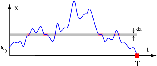
Figure 1: Schematic trajectory of a diffusing particle in space time that starts at $x_{0}$ and is absorbed at time $T_{0}$ (square). The time $T(x)$ that the particle spends in $[x,x+dx]$ is indicated by the colored segments.

Two basic questions about an excursion are: (i) What is its shape [6, 7]? (ii) How much time does the excursion spend in the range $[x,x+dx]$ before being absorbed? We term this latter quantity as the residence time. The properties of the residence time have been addressed in the mathematics literature by local-time theorems [8, 4, 9, 10] that specify the time that a Brownian particle spends in the region $[x,x+dx]$ before being absorbed when the origin is reached. When $x<x_{0}$, the distribution of this residence time was shown to be related to the distribution of the radial distance of a two-dimensional Brownian motion [9, 10]. If the particle wanders in a finite domain with reflection at the domain boundary and absorption at a given point (or points) within the domain, the residence time at each site is related to the first-passage time to the absorbing set [11, 12, 13]. This general formalism allows one to compute both the average residence time and the distribution of residence times at a given location.

While the consequences of local-time theorems are profound, the mathematical literature is sometimes presented in a style that is not readily accessible to the community of physicists who study random walks, and some of the results derived in Refs. [11, 12, 13] are extremely general in their formulation. In this work, we investigate residence-time phenomena for both continuum diffusion and the discrete random walk by using simple ideas and approaches from first-passage processes. We focus on cases where the particle is eventually absorbed at a specified boundary (e.g., one specific side of an interval) and/or starts close to this boundary. Some of these situations have been treated previously in Ref. [14], by a more formal approach than that presented here.

In Sec. 2.1, we first derive the average residence time within the interval $[x,x+dx]$ in continuum diffusion, by solving the relevant diffusion equation. We extend this approach to: (a) biased diffusion on the semi-infinite line (Sec. 2.2), and (b) unbiased diffusion in a finite domain $[0,L]$, with the condition that the particle is eventually absorbed at $x=0$ (Sec. 2.3). We then determine the average residence time in general spatial dimension in the domain exterior to an absorbing sphere of radius $a$ (Sec. 2.4).

We then turn to the corresponding discrete system of a nearest-neighbor symmetric random walk that starts at $x_{0}=1$ and is absorbed when $x=0$ is reached. The analog of the residence time is the number of times that the walk revisits a given point $x$ before it dies at $x=0$. We write the total number of steps of this random walk—which is necessarily odd—as $2n+1$. In Sec. 3, we use generating function methods to derive the average number of visits to a given site for a symmetric random walk on the semi-infinite line. For fixed $n$, we will show that the average number of times that $x=1$ is revisited equals $3n/(n+2)$. By averaging this quantity over the total number of steps of the walk, we will show that there are, on average, 2 revisits to $x=1$. Moreover, the average number of times that the random walk visits a site at $x>1$ equals 4 for any $x>1$. These results match those found in continuum diffusion in the analogous geometry. Finally, in Sec. 4, we determine the time when a walk first revisits $x=1$, when it starts at $x=1$ and is eventually absorbed at $x=0$. We give some concluding comments in Sec. 5.

2 Residence Time for Diffusion

2.1 Isotropic diffusion on the semi-infinite line

Consider a particle with diffusion coefficient $D$ that starts at $x_{0}$ and is absorbed when $x=0$ is reached. For such a particle, the image method gives the probability density for the particle to be at position $x>0$ as [15, 16]

$$P(x,t)=\frac{1}{\sqrt{4\pi Dt}}\,\,\left[e^{-(x-x_{0})^{2}/4Dt}-e^{-(x+x_{0})^{2}/4Dt}\right]\,.$$ (1)

The time $T(x)$ that the particle, which starts at $x_{0}$, spends in the range $[x,x+dx]$ before being absorbed at $x=0$ (Fig. 1) is simply the integral of the probability density over all time times $dx$ (see Refs. [2, 3, 17, 18, 19] for related approaches). Performing this integral, with $P(x,t)$ from Eq. (1), the residence time $T(x)$ is given by

$$T(x)=dx\int_{0}^{\infty}\!dt\,P(x,t)=\begin{cases}{\displaystyle\frac{x}{D}}\,\,dx&\qquad x<x_{0}\,,\\[14.22636pt] {\displaystyle\frac{x_{0}}{D}}\,\,dx&\qquad x>x_{0}\,.\end{cases}$$ (2)

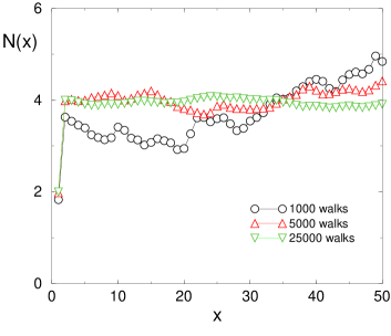
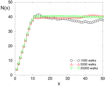
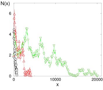
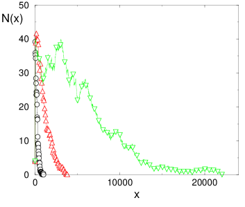
Figure 2: Simulation results for $N(x)$, the average number of times that a random walk visits $x$ when it starts at: (a) $x_{0}=1$, and (b) $x_{0}=10$. Here $N(x)$ is the discrete analog of the residence time $T(x)$. (c) & (d): The same data as in (a) and (b) over the full range of $x$.

To illustrate this result, we present simulations for a nearest-neighbor random walk that starts at: (a) $x_{0}=1$ and (b) at $x_{0}=10$ in Fig. 2. As a function of the number of walks in the ensemble, $T(x)$ slowly converges to the asymptotic time-independent value in Eq. (2). A curious feature of this residence-time data is that it becomes erratic for large $x$, as shown in Figs. 2(c) and (d). We can understand the origin of these large fluctuations by the following rough argument: for a diffusing particle that starts at $x_{0}$, the probability $S(t)$ that it survives until time $t$ is $S(t)=\text{erf}\big{(}x_{0}/\sqrt{4Dt}\big{)}\simeq x_{0}/\sqrt{4Dt}$ for $t\to\infty$ [16]. For $\mathcal{M}$ random walks, we estimate the longest lived of them by the extreme-statistics criterion $S(t_{\rm max})\simeq 1/{\mathcal{M}}$ [20, 21], which states that one out of $\mathcal{M}$ walks survives until at least time $t_{\rm max}$. This criterion gives $t_{\rm max}\simeq(\mathcal{M}x_{0})^{2}/4D$. Correspondingly, the maximal range reached by an ensemble of $\mathcal{M}$ random walks is, roughly, $x_{\rm max}\sim\sqrt{Dt_{\rm max}}\sim\mathcal{M}x_{0}$.

We now use this estimate to determine the large-$x$ fluctuations in Figs. 2(c) and (d). To obtain an accuracy of, say, 10%, in $N(x)$, the number of times that the lattice site at $x$ is visited by a random walk, we need roughly 100 walks to reach this value of $x$. Since $x_{\rm max}$ scales linearly in the number of realizations, roughly $m=100$ walks will reach a distance $x=\mathcal{M}x_{0}/m$. For example, for 25000 walks starting at $x_{0}=1$, roughly 100 of them will reach $x=250$. Thus up to $x\approx 250$, the variation in $N(x)$ should be smaller than 10%, and beyond this point fluctuations should become progressively more pronounced. This estimate is consistent with the data of Figs. 2(c) and (d).

The approach given here can be readily extended to any situation where the spatial probability distribution can be computed explicitly. We now investigate three such cases: (a) biased diffusion, (b) diffusion constrained to remain in the interval $[0,L]$, and (c) diffusion exterior to an absorbing sphere in general spatial dimension $d$.

2.2 Biased diffusion on the semi-infinite line

Suppose that a diffusing particle also experiences a constant bias velocity $-v$ that systematically pushes the particle towards the origin, so that the average time for the particle to reach the origin is finite. For a diffusing particle that starts at $x_{0}$, its probability density can be obtained by the image method [15, 16], and is given by

$$P(x,t)=\frac{1}{\sqrt{4\pi Dt}}\,\,\left[e^{-(x-x_{0}+vt)^{2}/4Dt}-e^{-vx_{0}/D}\,\,e^{-(x+x_{0}+vt)^{2}/4Dt}\right]\,.$$ (3)

Notice that the magnitude of the image particle is different from that of the initial particle, while the velocities of the initial and image particles are the same.

We again integrate this expression over all time and obtain, for the time that the particle spends in $[x,x+dx]$ before it dies:

$$T(x) =\begin{cases}{\displaystyle\frac{dx}{v}\left[1-e^{-vx/D}\right]}&\qquad x<x_{0}\,,\\[11.38109pt] {\displaystyle\frac{dx}{v}\,\,e^{-vx/D}\left[e^{vx_{0}/D}-1\right]}&\qquad x>x_{0}\,.\end{cases}$$ (4a)

For $$v\to 0 v\to\infty$$, Eq. (2) is recovered, while in the opposite limit of , (4a) reduces to

$$T(x)\to\begin{cases}{\displaystyle\frac{dx}{v}}&\qquad x<x_{0}\,,\\[14.22636pt] {\displaystyle\frac{dx}{v}\,\,e^{-v(x-x_{0})/D}}&\qquad x>x_{0}\,.\end{cases}$$ (4b)

As one might expect, the time spent in $[x,x+dx]$ with $x<x_{0}$ is just that of a ballistic particle, while it is exponentially unlikely for the particle to reach the classically forbidden region $x>x_{0}$ for large Péclet number, $vx/D$.

2.3 Diffusion in a finite interval

Suppose that an isotropically diffusing particle is constrained to remain within the interval $[0,L]$ and is eventually absorbed at $x=0$. We again want the time $T(x)$ that the particle spends in $[x,x+dx]$ before it dies. As in the previous two subsections, we need the spatial probability distribution for a diffusing particle with absorbing boundary conditions at $0$ and at $L$. A straightforward computation of this distribution is unwieldy, as it involves either an infinite Fourier series or an infinite number of images.

However, we can avoid this complication by noticing that we only want the integral of the probability distribution over all time, which corresponds to its Laplace transform at Laplace variable $s=0$. The Laplace transform satisfies $s\widetilde{P}-\delta(x-x_{0})=D\widetilde{P}_{xx}$, where $\widetilde{P}$ denotes the Laplace transform and the subscript denotes partial differentiation. For $s=0$, this reduces to the Laplace equation

$$D\widetilde{P}_{xx}=-\delta(x-x_{0})\,.$$

We solve this equation separately in the subdomains $x<x_{0}$ and $x>x_{0}$, impose the boundary conditions, continuity of the solution at $x=x_{0}$, and the joining condition $D\big{(}\widetilde{P}_{x}|_{>}-\widetilde{P}_{x}|_{<}\big{)}=-1$ to give, after standard steps,

$$\widetilde{P}=\frac{x_{<}}{D}\Big{(}1-\frac{x_{>}}{L}\Big{)}\,,$$ (5)

where $\widetilde{P}_{x}|_{>}$ is the derivative just to the right of $x_{0}$ (and similarly for $\widetilde{P}_{x}|_{<}$), and $x_{<}=\text{min}(x,x_{0})$, $x_{>}=\text{max}(x,x_{0})$.

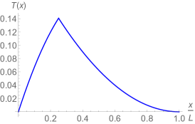
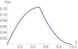
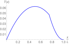
Figure 3: The residence time density $T(x)/dx$ for a diffusing particle that is constrained to remain within the interval $[0,L]$ until it exits at $x=0$. Shown are the cases: (a) $x_{0}=0.25L$, (b) $x_{0}=0.5L$ and (c) $x_{0}=0.75L$.

Finally, to obtain $T(x)$, we need to multiply the above distribution by the probability that the particle eventually exits the strip at $x=0$, which is simply $1-\frac{x}{L}$. Thus we have

$$T(x) =dx\,\int_{0}^{\infty}dt\,P(x,t)\left(1-\frac{x}{L}\right)=\widetilde{P}(x,s=0)\left(1-\frac{x}{L}\right)\,dx\,,$$

$$=\begin{cases}{\displaystyle\frac{x}{D}\Big{(}1-\frac{x_{0}}{L}\Big{)}\Big{(}1-\frac{x}{L}\Big{)}\,\,dx}&\qquad x<x_{0}\,,\\[11.38109pt] {\displaystyle\frac{x_{0}}{D}\Big{(}1-\frac{x}{L}\Big{)}^{2}\,\,dx}&\qquad x>x_{0}\,.\end{cases}$$ (6)

The maximum residence time occurs at $x=x_{0}$ for $x_{0}<{L}/{2}$ and then “sticks” at $x={L}/{2}$ for $x_{0}\geq{L}/{2}$, with a cusp always occurring at $x=x_{0}$ (Fig. 3). In the limit $L\rightarrow\infty$, we recover the result (2) for diffusion on the semi-infinite line.

2.4 Diffusion exterior to a sphere in dimension $d>2$

We now determine the residence time for a diffusing particle that wanders in the region exterior to an absorbing sphere of radius $a$, a geometry that is the analog of the semi-infinite system in one dimension. Without loss of generality, we take the initial condition to be a spherical shell of unit total probability at radius $r_{0}$. We first treat the case of spatial dimensions $d>2$ and then the special case of $d=2$.

For general $d$, we need to solve the Laplace equation

$$D\nabla^{2}\widetilde{P}=-\frac{1}{\Omega_{d}\,r_{0}^{d-1}}\,\,\delta(r-r_{0})\,,$$ (7)

where $\Omega_{d}$ is the surface area of a $d$-dimensional unit sphere and $r_{0}$ is the radial coordinate of the starting point. Because of the spherically symmetric source term, angular coordinates are irrelevant. We therefore separately solve $\widetilde{P}^{\prime\prime}+\frac{d-1}{r}\widetilde{P}^{\prime}=0$ in the subdomains $a<r<r_{0}$ and $r_{0}<r$, and then impose the absorbing boundary condition at $r=a$ and the joining condition by integrating (7) over an infinitesimal interval that includes $x_{0}$. The result of these standard manipulations is

$$\widetilde{P}(r)=\frac{1}{D(2-d)\Omega_{d}}\left[\Big{(}\frac{r_{<}}{a}\Big{)}^{2-d}-1\right]r_{>}^{2-d}\,.$$ (8)

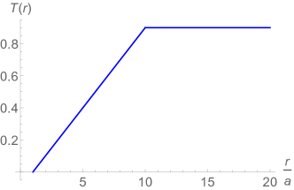
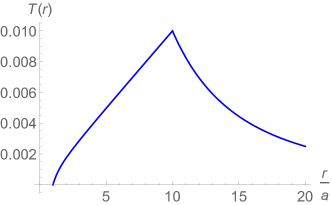
Figure 4: The residence time density $T(r)/dr$ for a diffusing particle that starts at $r_{0}=10$ exterior to a sphere of radius 1 in: (a) $d=3$ and (b) $d=5$.

To obtain $T(r)$, the residence time in a shell of radius $r$ and thickness $dr$, we again need to multiply the above expression by the probability that the particle eventually hits the sphere, which, for $d>2$, is simply $(a/r)^{d-2}$ [16]. Thus we have

$$T(r) =\Omega_{d}\,r^{d-1}\widetilde{P}(r)\,\Big{(}\frac{a}{r}\Big{)}^{d-2}dr\,,$$

$$=\begin{cases}{\displaystyle\frac{dr}{D(d-2)}\Big{(}\frac{a}{r}\Big{)}^{d-2}\Big{[}1-\Big{(}\frac{a}{r}\Big{)}^{d-2}\Big{]}\frac{r^{d-1}}{r_{0}^{d-2}}}&\qquad r<r_{0}\,,\\[17.07164pt] {\displaystyle\frac{dr}{D(d-2)}\,\Big{(}\frac{a}{r}\Big{)}^{d-2}\Big{[}1-\Big{(}\frac{a}{r_{0}}\Big{)}^{d-2}\Big{]}\,r}&\qquad r>r_{0}\,.\end{cases}$$ (9)

Two representative results are shown in Fig. 4. For large spatial dimension, a particle that eventually hits the sphere of radius $a$ must do so quickly. Thus the residence time in the domain $r>r_{0}$ must necessarily be small, as shown in Fig. 4(b) for $d=5$.

In spatial dimension $d=2$, the result analogous to Eq. (8) is

$$\widetilde{P}(r)=\frac{1}{2\pi D}\,\ln\frac{r_{<}}{a}\,.$$ (10)

In distinction to the cases of $d=1$ and $d>2$, $\widetilde{P}(r)$ is constant for $r>r_{0}$. Since a diffusing particle always reaches the absorbing sphere in $d=2$, we immediately have $T(r)=2\pi r\widetilde{P}(r)\,dr$.

3 Visitation by a Discrete Random Walk

We now investigate the corresponding residence time for a symmetric random walk in the semi-infinite one-dimensional domain $[0,\infty]$. The walk starts at lattice site $x_{0}$ and is absorbed when it first reaches $x=0$. The analog of the residence time is $N(x)$, the number of times that the random walk visits site $x$ (excluding the initial visit if $x=x_{0}$) before the walk dies. We use the generating function approach to derive this quantity for the case of $x_{0}=1$.

3.1 Average number of revisits to $x=1$

For a random walk that starts at $x_{0}=1$ and is absorbed at $x=0$, the number of steps in the walk is necessarily odd. For convenience, we write this number as $2n+1$, with $n$ an arbitrary non-negative integer. We define $A(n,k)$ as the number of random-walk paths that start at $x_{0}=1$, take the first step to the right (thus upward in the space-time representation of Fig. 5), and make $k$ revisits to $x=1$, before dying at the $(2n+1)$st step. The number of such paths was found in [22] and is given by

$$A(n,k)=\frac{k\,(2n-k-1)!}{(n-k)!\,n!}\,,$$ (11)

which happens to be directly related to the triangular Catalan numbers [23, 24]. To compute the average number of revisits to $x=1$, we will need $\mathbf{P}(k\,|\,n)$, the conditional probability for a path to make exactly $k$ revisits to $x=1$ before dying at step $2n+1$. This probability is

$$\mathbf{P}(k\,|\,n)={A(n,k)}/{C_{n}}\,,$$ (12)

where $C_{n}=\frac{1}{n+1}\binom{2n}{n}$ is the $n$th Catalan number [25], which counts the total number of random walks of $2n$ steps that start at $x=0$, remain in the region $x\geq 0$, and return to $x=0$ at step $2n$. For what follows, we will also need

$$P(n)=C_{n}/2^{2n}\,,$$ (13)

the probability that a random walk first returns to its starting point at step $2(n+1)$. Note the shift $n\to n+1$ to ensure that the walk always remains above $x=0$.

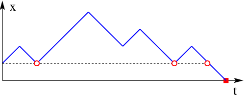
Figure 5: Space-time trajectory of a one-dimensional random walk of $2n+1=13$ steps that starts at $x=1$ and makes 3 revisits to $x=1$ (red circles) before being absorbed at $x=0$ (square). This path contributes to $A(6,3)$ (see Eq. (11)).

From Eqs. (11) and (12), we have

$$\mathbf{P}(k\,|\,n)=\frac{k\,(2n-k-1)!\,(n+1)!}{(n-k)!\,(2n)!}=k\,{\binom{n+1}{k+1}}\bigg{/}{\binom{2n}{k+1}}\,.$$ (14)

Thus the number of revisits to $x=1$, averaged over all walks of $2n+1$ steps is given by

$$\langle k\rangle_{n}=\sum_{k=1}^{\infty}\,k\,\mathbf{P}(k\,|\,n)\,.$$ (15)

Using expression (14) for $\mathbf{P}(k\,|\,n)$ in the above average, we obtain the remarkably simple result

$$\langle k\rangle_{n}=\sum_{k=1}^{\infty}\,k^{2}\,{\binom{n+1}{k+1}}\bigg{/}{\binom{2n}{k+1}}=\frac{3n}{n+2}\,.$$ (16)

For long paths of $2n+1$ steps, there are, on average, $3$ revisits to $x=1$, after which the walk immediately dies.

We now determine the number of revisits to $x=1$ upon also averaging over all $n$. This double average is

$$\langle\!\langle k\rangle\!\rangle=\sum_{n,k\geq 1}k\,\mathcal{P}(n,k)\,.$$ (17)

Here $\mathcal{P}(n,k)$ is the joint probability that the walk first reaches $x=0$ at step $2n+1$, and the walk makes $k$ revisits to $x=1$ within $2n+1$ steps. This joint probability is

$$\mathcal{P}(n,k)=\mathbf{P}(k\,|\,n)\,P(n)=\frac{A(n,k)}{C_{n}}\,\frac{C_{n}}{2^{2n}}=\frac{A(n,k)}{2^{2n}}\,.$$ (18)

The average in (17) may now be expressed in terms of the generating function for $\mathcal{P}(n,k)$:

$$g(x,y)=\sum_{n,k\geq 1}\,\mathcal{P}(n,k)\,x^{n}\,y^{k} =\sum_{n,k\geq 1}\,\frac{1}{2^{2n}}\,A(n,k)\,x^{n}\,y^{k}\,,$$

$$=\sum_{n,k\geq 1}\,\frac{1}{2^{2n}}\,\frac{(2n-k-1)!\,k}{(n-k)!\,n!}\,x^{n}\,y^{k}\,,$$

$$=\frac{xy}{2-xy+2\sqrt{1-x}}\,,$$ (19)

Which was derived in [22] (see also [26]). In terms of the generating function, we immediately obtain the remarkably simple result

$$\langle\!\langle k\rangle\!\rangle=\sum_{n,k\geq 1}\,k\,\mathcal{P}(n,k)\,x^{n}\,y^{k}\,\Big{|}_{(1,1)}=y\,\,\frac{\partial g}{\partial y}\,\bigg{|}_{(1,1)}\!\!=2\,.$$ (20)

There are, on average, 2 revisits to $x=1$ in the ensemble of all random walks that start at $x=1$, take their first step to the right, and are eventually absorbed at $x=0$.

We can extend Eq. (16) to higher integer moments of the average number of revisits to $x=1$ for walks of $2n+1$ steps. The first few of these fixed-$n$ moments are:

$$\langle k^{2}\rangle_{n} =\frac{n(13n-1)}{(2+n)(3+n)}\,,$$

$$\langle k^{3}\rangle_{n} =\frac{15n^{2}(5n-1)}{(2+n)(3+n)(4+n)}\,,$$

$$\langle k^{4}\rangle_{n} =\frac{541n^{2}-196n^{2}+11n^{2}+4n}{(2+n)(3+n)(4+n)(5+n)}\,,$$ (21a)

etc. We can similarly compute the higher integer moments of the number of revisits to $$x=1$$, averaged over all walk lengths, and the first few are:

$$\langle\!\langle k^{2}\rangle\!\rangle=6\qquad\langle\!\langle k^{3}\rangle\!\rangle=26\qquad\langle\!\langle k^{4}\rangle\!\rangle=150\qquad\langle\!\langle k^{5}\rangle\!\rangle=1082\,,$$ (21b)

etc. Parenthetically, these numbers are also sequence A000629 in the On-Line Encyclopedia of Integer Sequences [27]

In the next section, we will also need the generating function when the first step of the walk can equiprobably be to the right or to the left. This leads to the possibility that the total number of steps $2n+1=1$, i.e., $n=0$, for which the number of revisits to $1$ equals zero. The generating function for the joint probability $\mathcal{P}(n,k)$ for this ensemble of random walks therefore is

$$G(x,y)=\sum_{n,k\geq 0}\,\mathcal{P}(n,k)\,x^{n}\,y^{k} =\tfrac{1}{2}\big{[}1+g(x,y)\big{]}\,,$$

$$=\frac{1}{2}\left(1+\frac{xy}{2-xy+2\sqrt{1-x}}\right)\,,$$ (22)

where the term 1 in the parenthesis comes from the walk that initially steps to the left and is immediately absorbed. Notice that $y\frac{\partial G}{\partial y}\big{|}_{(1,1)}=1$, which is consistent with (3.1): half of all paths die immediately upon the first step, and thus never return to $1$, while the other half return twice, on average, as derived in (20).

3.2 Average number of visits to $x=2$

We now extend the above approach to a walk that starts at $x=1$ and is constrained to take its first step to the right, to determine the number of visits to $x=2$. For this purpose, we define three random variables that characterize this set of walks:

• $2n+1$, the total number of steps in the walk when it dies;

• $k$, the number of visits to $x=2$ (including the first visit);

• $\ell$, the number of excursions that lie above the level $x=1$.

Since an excursion is a path that lies between two successive returns to $x=1$ (and thus always remains above $x=1$), the minimal length excursion is the path $1\to 2\to 1$.

We want the ensemble average of the number of visits to $x=2$. To facilitate this calculation, it is useful to define the three-variable generating function

$$\mathcal{G}(x,y,z)=\sum_{n\geq 1}\,\sum_{1\leq\ell\leq n}\,\sum_{\ell\leq k\leq n}\,\mathcal{P}\left(n,k,\ell\right)\,x^{n}\,y^{k}\,z^{\ell}\,,$$ (23)

which encodes all paths according to $(n,k,\ell)$. We also label each successive excursion of the path above $x=1$ by the index $1\leq i\leq\ell$, and we introduce the variables $2m_{i}$ and $j_{i}$, respectively, for the number of steps in the $i$th such excursion, and the number of returns to $x=2$ in this excursion (Fig. 6). As shown in this figure, $2m_{i}$ counts the number of steps that lie above $x=2$. Thus for an excursion that goes from $x=1$ to $x=2$ and immediately returns to $x=1$, $m_{i}=0$. In addition, $j_{i}$ counts the number of revisits to $2$, so that the total number of visits to $x=2$ in the $i$th excursion above $x=1$ is $j_{i}+1$. The variables $j_{i}$, $m_{i}$, and $\ell$ must satisfy the geometric constraints (see Fig. 6):

$$\begin{split}&j_{1}+j_{2}+\dots+j_{\ell}+\ell=k\,,\\ &m_{1}+m_{2}+\dots+m_{l}+\ell=n\,,\\ &j_{i}\leq m_{i}\,.\end{split}$$ (24)

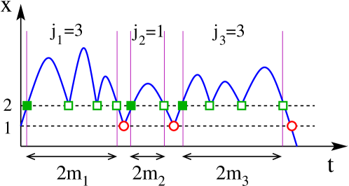
Figure 6: Schematic space-time trajectory of a random walk that starts at $x=1$ and has 3 revisits to $x=1$ (red circles) and $k=10$ visits to $x=2$ (green squares). There are $\ell=3$ excursions above $x=1$. Immediately after a revisit to $x=1$, the next revisit to $x=2$ is shown as a solid green square.

Using these definitions, the three-variable generating function $\mathcal{G}(x,y,z)$ can be functionally expressed in terms of $G(x,y)$ defined in Eq. (3.1) as (see the Appendix for details of this derivation)

$$\mathcal{G}(x,y,z)=\sum_{\ell\geq 1}\,P(\ell)\,\left[x\,y\,z\,G(x,y)\right]^{\ell}\,,$$ (25)

where $P(\ell)$ is the probability that there are $\ell$ excursions above $x=1$ averaged over walks of any length, which is also the distribution of the number of returns to $x=1$.

One may compute $P(\ell)$ as the marginal of the joint distribution of the number of steps and the number of excursions:

$$P(\ell)=\sum_{n\geq 1}\mathcal{P}(n,\ell)=\sum_{n\geq 1}\frac{1}{2^{2n}}\,A(n,\ell)\,.$$ (26)

The above sum starts at $n=1$ because we are imposing the condition that the first step of the walk is to the right. Consequently the three-variable generating function in (25) will ultimately be expressed in terms of the restricted generating function $g$. Substituting Eq. (26) in (25) and comparing the resulting formula with the first line of (3.1), we obtain

$$\mathcal{G}(x,y,z) =\sum_{\ell\geq 1}\,P(\ell)\,\big{[}x\,y\,z\,G(x,y)\big{]}^{\ell}$$

$$=\sum_{\ell\geq 1}\,\sum_{n\geq 1}\frac{1}{2^{2n}}\,A(n,\ell)\,\big{[}x\,y\,z\,G(x,y)\big{]}^{\ell}$$

$$=g\big{(}1,x\,y\,z\,G(x,y)\big{)}\,.$$ (27)

It is now straightforward to calculate $\langle k\rangle$. From the definition of the generating function (23), we have

$$\langle k\rangle =y\,\frac{\partial\mathcal{G}}{\partial y}\Big{|}_{x=y=z=1}\,,$$

$$=y\,\frac{\partial g}{\partial y}\Big{|}_{x=y=1}\ \left[G(1,1)+y\frac{\partial G}{\partial y}\Big{|}_{x=y=1}\right]\,,$$

$$=2\times\left(1+1\right)\,,$$

$$=4\,.$$ (28)

A random walk thus visits $x=2$ twice as often as $x=1$, as already predicted by the continuum solution (2).

3.3 Average number of visits to $x>2$

The ensemble average of the number of visits to a given level $x>2$ may be readily computed by induction. We start by calculating the average number of visits to $x=3$, and it will become apparent that this approach applies for any $x>2$. Each time a random walk reaches $x=2$, there are two possibilities at the next step: the walk may step forward to $x=3$ or step back to $x=1$. Let us first assume that the walk goes to $x=3$, which occurs with probability $\frac{1}{2}$. Each time this event occurs, we now ask: what is the average number of visits to $x=3$ (including this first visit) before the walk returns to $x=2$?

With probability $\frac{1}{2}$, the walk may immediately return to $x=2$, in which case, there is one visit to $x=3$. On the other hand, if the walk steps to $x=4$, we have the same situation as that discussed in Sec. 3.1. Namely, if we view $x=3$ as the starting point, we know that there are 2 revisits to $x=3$ and thus 3 visits to $x=3$, on average, before the walk steps back to $x=2$. Thus each time $x=3$ is reached, there are

$$\Big{(}\frac{1}{2}\times 1\Big{)}+\Big{(}\frac{1}{2}\times 3\Big{)}=2$$

two visits, on average, to $x=3$.

For a walk that reaches $x=2$, the average number of visits to $x=3$ for this visit to $x=2$ therefore is

$$\Big{(}\frac{1}{2}\times 0\Big{)}+\Big{(}\frac{1}{2}\times 2\Big{)}=1\,.$$

The first term corresponds to the contribution from a walk that steps from $x=2$ to $x=1$ without hitting $x=3$, and the second term is the contribution when the walk steps from $x=2$ to $x=3$.

To summarize, each time the walk visits $x=2$, there is, on average, one visit to $x=3$, before the walk is at $x=2$ again. Clearly, this reasoning that determines the number of visits to $x+1$ for each visit to $x$ applies inductively for any level $x>2$. Thus we conclude that the average number of times that a random walk visits a given level $x>2$, equals 4, in agreement with the simulation results in Fig. 2(a). Clearly, our argument also applies for any starting point of the walk $x_{0}$, as long as we restrict to coordinates with $x>x_{0}+1$.

4 Time of the First Revisit

In addition to the number of revisits to $x=1$ by a random walk excursion that starts at $x=1$ and is eventually absorbed, we are interested in the time at which the first revisit occurs. This time characterizes the shape of the space-time trajectory of a random walk. Since the walk starts at $x=1$ and ends at $x=0$, its space-time shape is essentially that of a Brownian excursion — a Brownian trajectory that starts at $x=0$, remains above $x=0$ for all $0<t<T$, and returns to $x=0$ for the first time at $t=T$. The average shape of a Brownian excursion has been shown to be semi-circular [6, 7]. From this shape, we might anticipate that the first revisit to $x=1$ is unlikely to occur for $t$ near $T/2$ because such a revisit involves a large fluctuation from the average trajectory. Instead, it seems more likely that the first revisit to $x=1$ will occur either near the beginning or the end of the excursion, a feature that evokes the famous arcsine laws [1, 4]. We now show that this expectation is correct.

4.1 Time of first return to $1$ for fixed walk length $n$

Consider a random walk that starts at $x=1$, takes its first step to the right, and is absorbed at $x=0$ after $T=2n+1$ steps. What is the probability $P(2m\,|\,T)$ that such a walk revisits $x=1$ for the first time at step $\tau_{1}=2m$? Since the walk necessarily revisits $x=1$ at step $2n$ by definition, and the walk could revisit $x=1$ immediately after $2$ steps, $m$ satisfies the constraint $1\leq m\leq n$. The number of walks that revisit $x=1$ after $2m$ steps may be obtained by decomposing the full path into two constituents (Fig. 7):

• Excursions of $(2m-2)$ steps that wander in the domain $x\geq 2$ — the number of such paths is $C_{m-1}$;

• Excursions of $(2n-2m)$ steps that wander in the domain $x\geq 1$ — the number of such paths is $C_{n-m}$.

The first part accounts for the first return to $x=1$ at step $2m$ and the second part accounts for the remaining path of $2n-2m$ steps.

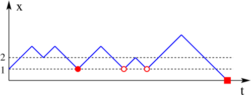
Figure 7: Space-time trajectory of a one-dimensional random walk of $2n+1=19$ steps that starts at $x=1$ and first revisits $x=1$ at step $2m=6$ (solid circle). Subsequent revisits to $x=1$ are indicated by open circles and the walk is absorbed when it first reaches $x=0$ (square).

The required probability is then simply the product of these two numbers divided by the total number of walks that start at $x=1$ and are absorbed after $2n+1$ steps, which is $C_{n}$. Therefore

$$\mathbf{P}\left(2m\,|\,T\right)=\frac{C_{m-1}\,C_{n-m}}{C_{n}}=\frac{n+1}{m\,(n-m+1)}\frac{\binom{2m-2}{m-1}\,\binom{2n-2m}{n-m}}{\binom{2n}{n}}\,.$$ (29)

Because $\mathbf{P}\left(\tau_{1}=2m\,|\,T=2n+1\right)$ is symmetric under $m\rightarrow n+1-m$, the average value of $\tau_{1}$, the time of the first revisit, conditioned on $T=2n+1$, can be immediately seen to be

$$\langle\tau_{1}\rangle_{n}=n+1\,.$$ (30)

The above result may also be obtained by direct calculation. Because of the bimodal nature of the underlying probability distribution, the average value is very different from the typical value. The average corresponds to the minimum of the probability distribution (Fig. 8(a)), just as in the arcsine law for the time of the last zero of a Brownian motion.

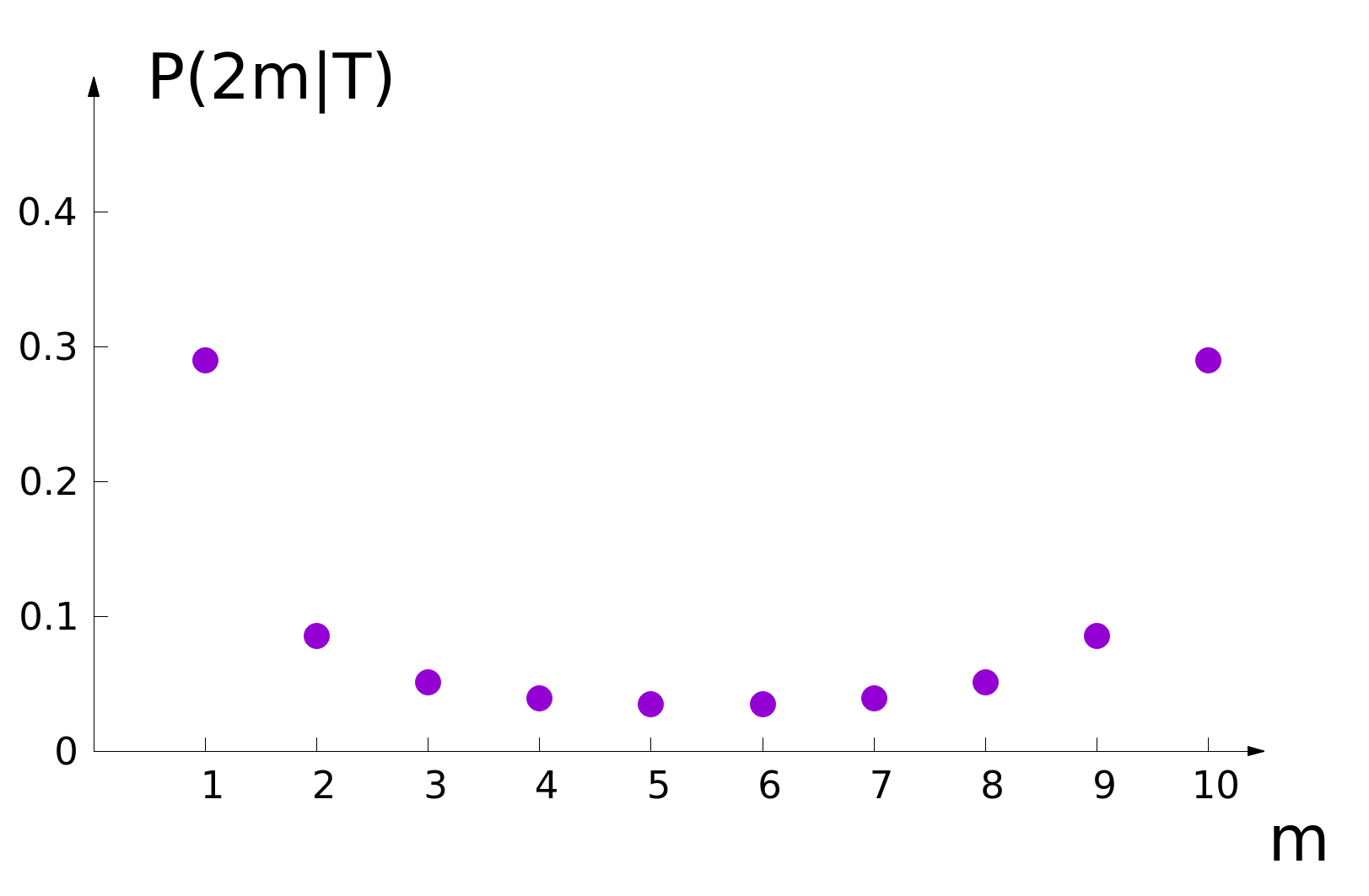
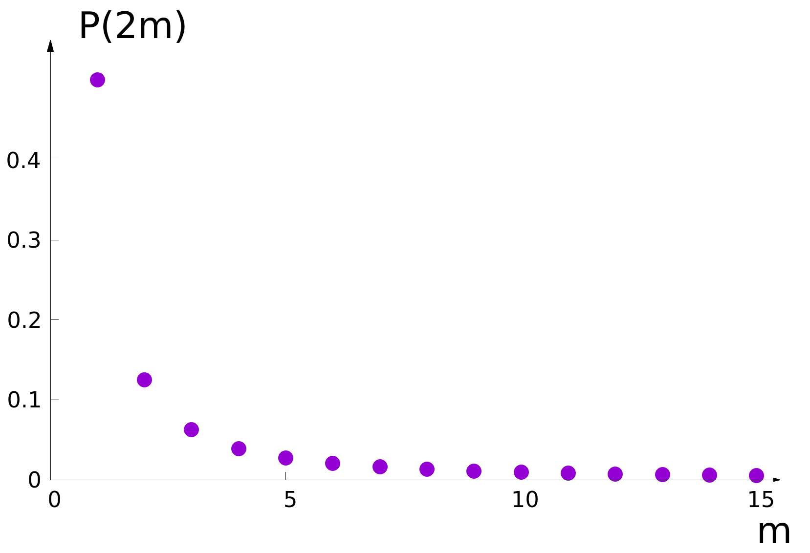
Figure 8: (a) Conditional distribution $P\left(\tau_{1}=2m\,|\,T=2n+1\right)$ for $n=10$. Note that typical (i.e. most likely) values of $\tau_{1}$ are $2$ and $2n$, while the average value is $\langle\tau_{1}\rangle=n+1$. (b) Distribution $P\left(\tau_{1}=2m\right)$ of the first revisit time to $1$.

4.2 Time of first return to $1$ for any $n$

From the conditional probability $\mathbf{P}\left(2m\,|\,T\right)$, we may now compute the joint probability $\mathcal{P}\left(2m,T\right)$:

$$\mathcal{P}\left(2m,T\right) =\mathbf{P}\left(2m\,|\,T\right)\,P(T)$$

$$=\frac{C_{m-1}\,C_{n-m}}{C_{n}}\times\frac{C_{n}}{2^{2n}}=\frac{C_{m-1}\,C_{n-m}}{2^{2n}}.$$ (31)

With this result, we can readily obtain the distribution $P(2m)$, the probability for a path of any length to perform an excursion of $2m$ steps that lies above $x=2$ between steps $1$ and $2m-1$ (with the first step constrained to go from $x=1$ to $x=2$):

$$P(2m) =\sum_{n\geq m}\,\mathcal{P}\left(2m,T\right)$$

$$=C_{m-1}\,\sum_{n\geq m}\,\frac{C_{n-m}}{2^{2n}}=\frac{C_{m-1}}{2^{2m-1}}\,.$$ (32)

This distribution is normalized, because $\sum_{m\geq 1}C_{m-1}/2^{2m-1}=1$. The Markovian nature of the random walk means that there is no memory between what happens after step $2m$ and the probability that the walk first revisits $x=1$ at step $2m$. Hence $P(2m)$ is simply the probability that a symmetric random walk first returns to its starting point at step $2m$, which asymptotically scales as $m^{-3/2}$ [1, 16, 4]. Because of this scaling, the average time for the first return, $\langle\!\langle\tau_{1}\rangle\!\rangle=\sum_{m}2m\,P(2m)$, is infinite, even though $P(2m)$ is peaked at $m=1$ (Fig. 8(b)).

5 Summary

We showed how standard first-passage methods can be used to determine the average time that a diffusing particle spends in a given spatial range when the particle starts at some point $x_{0}$ and dies when it reaches an absorbing point or set. We also derived corresponding results for the discrete random walk, where the analog of the residence time is the number of times that a given point is visited. For continuum diffusion, the average residence time in a given spatial range is simply the integral of the probability distribution over all time in this same range, with the given initial condition and the absorbing boundary condition. This perspective allowed us to also treat, in a relatively simple manner: (a) biased diffusion, (b) diffusion in a finite interval (conditioned on absorption at a given side of the interval), and (c) diffusion in general spatial dimensions. It is also worth emphasizing the time integral of the probability distribution at a given point is essentially just the electrostatic potential at this point. This correspondence provides a simple way to calculate residence times and to understand the dependence of the residence time on basic parameters.

The main qualitative feature of the residence time at a given point is that it vanishes (often linearly) in the distance between this point and the absorber. That is, a diffusing particle does not linger when it is close to an absorbing point. Another interesting feature, almost intuitive from the analogy with electrostatics, is the fact that, in low dimensions ($d\leq 3$), the average residence time at any point beyond the starting point is constant and simply equal to the average residence time at the starting point. This is no longer the case for $d\geq 4$, with an abrupt transition between $d=3$ and $d=4$. It would be of interest to understand why this transition occurs at a spatial dimension that differs from that of the well known transition between recurrence and transience, which happens at $d=2$.

For the discrete random walk, we exploited the generating function method to derive parallel results for the number of times that a given lattice site is visited before the walk dies at the absorbing point. For a walk that starts at $x_{0}=1$, there are, upon averaging over walks of all possible lengths, two subsequent visits to $x=1$ and four subsequent visits to $x=2$ before the random walk dies. We also showed that the random walk makes four subsequent visits to any point $x\geq 2$, on average. We also found that the first revisit to $x=1$ occurs near the start or the end of the path. This means that it is very unlikely that there will be a large deviation toward the boundary and away from the average position of the path near the middle of an excursion. This suggests that an individual Brownian excursion always remains close to its average shape. We hope to investigate this behavior in future work, with a view to obtaining a full characterization of the fluctuations around an excursion’s average semi-circular shape.

Appendix A Relation Between Generating Functions

Using the geometric constraints (24) in Eq. (23), the generating function $\mathcal{G}(x,y,z)$ can be re-expressed as

$$\mathcal{G}(x,y,z) =\sum_{n=1}^{\infty}\,\sum_{\ell=1}^{n}\,\sum_{k=\ell}^{n}\,\mathcal{P}\left(n,k,\ell\right)\,x^{n}\,y^{k}\,z^{\ell}$$

$$=\sum_{n=1}^{\infty}\,\sum_{\ell=1}^{n}\,\sum_{k=\ell}^{n}\,P(\ell)\,\mathbf{P}\left(n,k|\ell\right)\,x^{n}\,y^{k}\,z^{\ell}\,,$$ (33)

where we use $\mathbf{P}(\dots|\dots)$ to denote the conditional joint probability.

Next we write $\mathbf{P}\left(n,k|\ell\right)$ in terms of the variables $m_{i}$ and $j_{i}$ (see Fig. 6):

$$\mathcal{G}(x,y,z) =\sum_{n=1}^{\infty}\,\sum_{\ell=1}^{n}\,\sum_{k=\ell}^{n}\sum_{\begin{subarray}{c}j_{1}+\dots+j_{\ell}=k-\ell\\ m_{1}+\dots+m_{\ell}=n-\ell\\ j_{i}\leq m_{i}\end{subarray}}P(\ell)\,\mathbf{P}\left(m_{1},\dots,m_{\ell},j_{1},\dots,j_{\ell}|\ell\right)\,x^{m_{1}+\dots m_{\ell}+\ell}\,y^{j_{1}+\dots j_{\ell}+\ell}\,z^{\ell}$$

$$=\sum_{n=1}^{\infty}\,\sum_{\ell=1}^{n}\,\sum_{\begin{subarray}{c}m_{1}+\dots+m_{\ell}=n-\ell\\ 0\leq j_{i}\leq m_{i}\end{subarray}}\,P(\ell)\,\mathbf{P}\left(m_{1},\dots,m_{\ell},j_{1},\dots,j_{\ell}|\ell\right)\,x^{m_{1}+\dots m_{\ell}+\ell}\,y^{j_{1}+\dots j_{\ell}+\ell}\,z^{\ell}$$

$$=\sum_{\ell\geq 1}\,P(\ell)\,\sum_{n\geq\ell}\,\sum_{\begin{subarray}{c}m_{1}+\dots+m_{\ell}=n-\ell\\ 0\leq j_{i}\leq m_{i}\end{subarray}}\,\mathbf{P}\left(m_{1},\dots,m_{\ell},j_{1},\dots,j_{\ell}|\ell\right)\,x^{m_{1}+\dots m_{\ell}+\ell}\,y^{j_{1}+\dots j_{\ell}+\ell}\,z^{\ell}$$

$$=\sum_{\ell\geq 1}\,P(\ell)\,\sum_{m_{1},\dots,m_{\ell}\geq 0}\,\sum_{j_{1},\dots,j_{\ell}=0}^{m_{1},\dots,m_{\ell}}\,\left[\prod_{i=1}^{\ell}\,\mathbf{P}\left(m_{i},j_{i}|\ell\right)\,x^{m_{i}}\,y^{k_{i}}\right]\,(xyz)^{\ell}$$

$$=\sum_{\ell\geq 1}\,P(\ell)\,(xyz)^{\ell}\,\sum_{m_{1},\dots,m_{\ell}\geq 0}\,\sum_{j_{1},\dots,j_{\ell}=0}^{m_{1},\dots,m_{\ell}}\,\left[\prod_{i=1}^{\ell}\,\mathbf{P}\left(m_{i},j_{i}|\ell\right)\,x^{m_{i}}\,y^{j_{i}}\right]$$

$$=\sum_{\ell\geq 1}\,P(\ell)\,(xyz)^{\ell}\,\prod_{i=1}^{\ell}\left[\sum_{m_{i}\geq 0}\,\sum_{0\leq j_{i}\leq m_{i}}\,\,\mathbf{P}\left(m_{i},j_{i}|\ell\right)\,x^{m_{i}}\,y^{j_{i}}\right]\,.$$ (34)

We now use the fact that the random walk is a Markov process, which implies that $\mathbf{P}\left(m_{i},j_{i}|\ell\right)=\mathcal{P}\left(m_{i},j_{i}\right)=A(m_{i},j_{i})/2^{2m_{i}}$. Therefore

$$\sum_{m_{i}\geq 0}\,\sum_{0\leq k_{i}\leq m_{i}}\,\,\mathbf{P}\left(m_{i},j_{i}|\ell\right)\,x^{m_{i}}\,y^{j_{i}}=G(x,y)\,.$$ (35)

Note that $G(x,y)$, as defined in Eq. (3.1), appears here and not $g(x,y)$ because upon starting from $x=2$, when coming from $x=1$, the path is not conditioned to immediately move to $x=3$. In fact, the path is allowed to return immediately to $x=1$, as reflected in the fact that, for the $i$th excursion, $m_{i}$ may be $0$.
Eq. (34) becomes

$$\mathcal{G}(x,y,z)=\sum_{\ell\geq 1}\,P(\ell)\,(xyz)^{\ell}\,\prod_{1\leq i\leq\ell}\left[G(x,y)\right]=\sum_{\ell\geq 1}\,P(\ell)\,\left[x\,y\,z\,G(x,y)\right]^{\ell}\,.$$ (36)

This is Eq. (25) in the main text.

References

References

- [1] W. Feller, Introduction to Probability Theory and its Applications, 3rd ed., (J Wiley & Sons, Inc. New York, 1964).
- [2] F. Spitzer, Principles of Random Walk, (Van Nostrand, Princeton NJ, 1964)
- [3] E. W. Montroll and G. H. Weiss, J. Math. Phys. 6, 167 (1965).
- [4] P. Mörters and Y. Peres, Brownian Motion, (Cambridge University Press, Cambridge, UK, 2010).
- [5] K. L. Chung, Ark. Mat. 14, 155 (1976).
- [6] A. Baldassarri, F. Colaiori, and C. Castellano, Phys. Rev. Lett. 90, 060601 (2003).
- [7] F. Colaiori, A. Baldassarri, and C. Castellano, Phys. Rev. E 69, 041105 (2004).
- [8] P. Lévy, Processus stochastique et mouvement Brownien, (Gauthier-Villars, Paris, 1948).
- [9] D. Ray, Illinois Journal of Mathematics 7, 615 (1963)
- [10] F. B. Knight, Trans. Am. Math, Soc. 109, 56 (1963).
- [11] S. Condamin, V. Tejedor, and O. Bénichou, Phys. Rev. E 76, 050102 (2007).
- [12] O. Bénichou and J. Desbois, J. Phys. A: Math. Theor. 42, 015004 (2009).
- [13] O. Bénichou and R. Voituriez, Phys. Repts. 539, 225 (2014).
- [14] N. Agmon, J. Chem. Phys. 81, 3644 (1984).
- [15] H. E. Daniels, Ann. Statist. 10, 394 (1982).
- [16] S. Redner, A Guide to First-Passage Processes, (Cambridge University Press, Cambridge, UK, 2001).
- [17] M. Ferraro and L. Zaninetti, Phys. Rev. E 64, 056107 (2001).
- [18] M. Ferraro and L. Zaninetti, Physica A 338, 307 (2004).
- [19] M. Ferraro and L. Zaninetti, Phys. Rev. E 73, 057102 (2006).
- [20] J. Galambos, The Asymptotic Theory of Extreme Order Statistics, (Krieger, Malabar, FL, 1987).
- [21] P. L. Krapivsky, S. Redner, and E. Ben-Naim, A Kinetic View of Statistical Physics, (Cambridge University Press, Cambridge UK, 2010).
- [22] U. Bhat, S. Redner and O. Bénichou, J. Stat. Mech. 073213 (2017).
- [23] D. F. Bailey, Math. Mag. 69, 128 (1996) (http://www.jstor.org/stable/269067).
- [24] K.-H. Lee and S.-J. Oh, arXiv:1601.06685.
- [25] R. P. Stanley, Catalan Numbers, (Cambridge University Press, Cambridge UK, 2015).
- [26] R. P. Stanley, Enumerative Combinatorics vol. 2, (Cambridge University Press, Cambridge UK, 1999).
- [27] The On-Line Encyclopedia of Integer Sequences, https://oeis.org.