Assumption Lean Regression

Abstract

It is well known that models used in conventional regression analysis are commonly misspecified. A standard response is little more than a shrug. Data analysts invoke Box’s maxim that all models are wrong and then proceed as if the results are useful nevertheless. In this paper, we provide an alternative. Regression models are treated explicitly as approximations of a true response surface that can have a number of desirable statistical properties, including estimates that are asymptotically unbiased. Valid statistical inference follows. We generalize the formulation to include regression functionals, which broadens substantially the range of potential applications. An empirical application is provided to illustrate the paper’s key concepts.

1 Introduction

It is old news that models are approximations and that regression analyses of real data commonly employ models that are misspecified in various ways. Conventional approaches are laden with assumptions that are questionable, many of which are effectively untestable (Box, 1976, Leamer, 1878; Rubin, 1986; Cox, 1995; Berk, 2003; Freedman, 2004; 2009). This note discusses some implications of an “assumption lean” reinterpretation of regression. In this reinterpretation, one requires only that the observations are i.i.d., realized at random according to a joint probability distribution of the regressor and response variables. If no model assumptions are made, then the parameters of fitted models need to be interpreted as statistical functionals, here called “regression functionals.”

For ease and clarity of exposition we begin with linear regression. Later we turn to other types of regression and show how the lessons from linear regression carry forward to the generalized linear model and even more broadly. We draw heavily on two papers by Buja et al. (2016a;b), a portion of which draws on early insights of Halbert White (1980a).

2 The Parent Joint Probability Distribution

For observational data, suppose there is a set of quantitative random variables that have a joint distribution $\boldsymbol{P}$, also called the “population,” that characterizes regressor variables $X_{1},\dots,X_{p}$ and a response variable $Y$. The distinction between regressors and the response is determined by the data analyst based on subject matter interest. These designations do not imply any causal mechanisms and or any particular generative models for $\boldsymbol{P}$. Unlike in linear models theory, the regressor variables are not interpreted as fixed: they are as random as the response and will treated as such.

We collect the regressor variables in a $(p\!+\!1)\times 1$ column random vector $\vec{\boldsymbol{X}}=(1,X_{1}\dots,X_{p})^{\prime}$ with a leading 1 to accommodate an intercept in linear models. We write $\boldsymbol{P}=\boldsymbol{P}_{\!\!Y,\vec{\boldsymbol{X}}}$ for the joint probability distribution, $\boldsymbol{P}_{\!\!Y|\vec{\boldsymbol{X}}}$ for the conditional distribution of $Y$ given $\vec{\boldsymbol{X}}$, and $\boldsymbol{P}_{\!\!\vec{\boldsymbol{X}}}$ for the marginal distribution of $\vec{\boldsymbol{X}}$. The only assumption made is that the data are realized i.i.d. from $\boldsymbol{P}$. The separation of the random variables into regressors and a response implies that there is interest in $\boldsymbol{P}_{\!\!Y|\vec{\boldsymbol{X}}}$. Hence, some form of regression analysis is applied. Yet, because the regressors are random variables, their marginal distribution $\boldsymbol{P}_{\!\!\vec{\boldsymbol{X}}}$ cannot be ignored.

3 Estimation Targets

As a feature of $\boldsymbol{P}$ or, more precisely, of $\boldsymbol{P}_{\!\!Y|\vec{\boldsymbol{X}}}$, there is a “true response surface” denoted by $\mu(\vec{\boldsymbol{X}})$. Most often, $\mu(\vec{\boldsymbol{X}})$ is the conditional expectation of $Y$ given $\vec{\boldsymbol{X}}$, $\mu(\vec{\boldsymbol{X}})=\boldsymbol{E}[Y|\vec{\boldsymbol{X}}]$, but there are other possibilities, depending on the context. For example, $\mu(\vec{\boldsymbol{X}})$ might be chosen to be the conditional median or some other conditional quantile of $Y$ given $\vec{\boldsymbol{X}}$. The true response surface is a common estimation target for conventional regression in which a data analyst assumes a specific parametric form. We will not proceed in this manner and will not make assumptions about what form $\boldsymbol{P}_{\!\!Y|\vec{\boldsymbol{X}}}$ actually takes. Yet, we will make use of standard ordinary least squares (OLS) fitting of linear equations. This approach reflects data analytic situations in which either deviations from linearity in $\mu(\vec{\boldsymbol{X}})$ may be difficult to detect with diagnostics, or in which the fitted linear formula is known to be a deficient approximation to $\mu(\vec{\boldsymbol{X}})$, and yet, OLS is employed because of underlying substantive theories, measurement requirements, or considerations of interpretability.

Fitting a linear function $l(\vec{\boldsymbol{X}})=\boldsymbol{\beta}^{\prime}\vec{\boldsymbol{X}}$ to $Y$ with OLS can be achieved mathematically at the population $\boldsymbol{P}$ without assuming that the response surface $\mu(\vec{\boldsymbol{X}})$ is linear in $\vec{\boldsymbol{X}}$:

$$\boldsymbol{\beta}(\boldsymbol{P})=\operatorname*{argmin}_{\boldsymbol{\beta}\in{\mathrm{I}\!\mathrm{R}}^{p+1}}\boldsymbol{E}[(Y-\boldsymbol{\beta}^{\prime}\vec{\boldsymbol{X}})^{2}].$$ (1)

The vector $\boldsymbol{\beta}=\boldsymbol{\beta}(\boldsymbol{P})$ is the “population OLS solution” and contains the “population coefficients.” Notationally, when we write $\boldsymbol{\beta}$, it is understood to be $\boldsymbol{\beta}(\boldsymbol{P})$. Similar to finite datasets, the OLS solution for the population can be obtained by solving a population version of the normal equations, resulting in

$$\boldsymbol{\beta}(\boldsymbol{P})=\boldsymbol{E}[\vec{\boldsymbol{X}}\vec{\boldsymbol{X}}^{\prime}]^{-1}\boldsymbol{E}[\vec{\boldsymbol{X}}Y].$$ (2)

Thus, one obtains the best linear approximation in the OLS sense to $Y$ as well as to $\mu(\vec{\boldsymbol{X}})$. As such, it should be useful without (unrealistically) assuming that $\mu(\vec{\boldsymbol{X}})$ is identical to $\boldsymbol{\beta}^{\prime}\vec{\boldsymbol{X}}$.

We have worked so far with a distribution/population $\boldsymbol{P}$, not data. We have, therefor, defined a target of estimation: $\boldsymbol{\beta}(\boldsymbol{P})$ obtained from (1) and (2) is the estimand of empirical OLS estimates $\hat{\boldsymbol{\beta}}$ obtained from data. This estimand is well-defined as long as the joint distribution $\boldsymbol{P}$ has second moments and the regressor distribution $\boldsymbol{P}_{\!\!\vec{\boldsymbol{X}}}$ is not perfectly collinear. That is, the second moment matrix $\boldsymbol{E}[\vec{\boldsymbol{X}}\vec{\boldsymbol{X}}^{\prime}]$ is full rank. No other assumptions are needed. In particular, there are no assumptions of linearity of $\mu(\vec{\boldsymbol{X}})$, homoskedasticity, or Gaussianity. This constitutes the “assumption lean” or “model robust” framework.

A foundational question is why one should settle for the best linear approximation to the truth. Indeed, those who insist that models must always be “correctly specified” will be unreceptive. They may insist that models should be revised until diagnostics and goodness of fit tests no longer detect deficiencies. One may then legitimately proceed as if the model is correct.

Such thinking warrants careful scrutiny. Data analysis with a given, fixed sample size requires decisions about how to balance the desire for good models against the costs of data dredging. “Improving” models by searching regressors, trying out transformations of all variables, inventing new regressors from existing ones, applying algorithms and interactive experiments, and undertaking assessments with diagnostic tests and plots can each invalidate subsequent statistical inference. The result often is models that not only fit the data well, but fit them too well (Hong et al. 2017).

Research is underway to provide valid post-selection inference (e.g., Berk et al. 2013, Lee et al. 2016), which is an important special case. But the proposed procedures address solely regressor selection and typically make strong assumptions. With these significant caveats, asymptotically valid post-selection inference under misspecification has substantial promise (Bachoc et al. 2016, Kuchibhotla et al. 2018), but there is not yet much to help the data analyst.

Beyond the costs of data dredging, there can be substantive reasons for curtailing “model improvement.” Some variables may express phenomena in “natural” or “conventional” units that should not be transformed even if model fit is improved. A substantive theory may require a particular model that does not fit the data well. Identifying important variables may be the primary concern, making quality of the fit less important. Predictors prescribed by subject-matter theory or past research may be unavailable so that the model specified is the best that can be done. In short, one must consider ways in which valid statistical inference can be undertaken with models acknowledged to be approximations.

Note that we are not making an argument for discarding model diagnostics. It is always important to learn what one can from the data, including model deficiencies that properly circumscribe conclusions being drawn. But there can be serious risks trying impose remedies that really are not.

We also are not simply restating Box’s maxim that models are always “wrong” in some ways but can useful despite their deficiencies. Acknowledging models as approximations is one thing. Understanding the consequences is another. What follows, therefore, is a discussion of some of these consequences and an argument in favor of assumption lean inference employing model robust standard errors, such as those obtained from sandwich estimators or the $x$-$y$ bootstrap.

4 A Population Decomposition of the Conditional Distribution of $Y$

A first step in understanding the statistical properties of the best linear approximation is to consider carefully the potential disparities in the population between $\mu(\vec{\boldsymbol{X}})$ and $\boldsymbol{\beta}^{\prime}\vec{\boldsymbol{X}}$. Figure 1 provides a visual representation. There is for the moment a response variable $Y$ and a single regressor $X$.

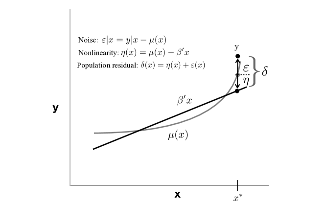
Figure 1: A Population Decomposition of $Y|X$ Using the Best Linear Approximation

The curved line shows the true response surface $\mu(x)$. The straight line shows the best linear approximation $\beta_{0}+\beta_{1}x$. Both are features of the joint probability distribution, not a realized dataset.

The figure shows a regressor value $x^{*}$ drawn from $\boldsymbol{P}_{\!\!\vec{\boldsymbol{X}}}$ and a response value $y$ drawn from $\boldsymbol{P}_{\!\!Y|X=x^{*}}$. The disparity between $y$ and the fitted value from the best linear approximation is denoted as $\delta=y-(\beta_{0}+\beta_{1}x^{*})$ and will be called the “population residual.” The value of $\delta$ at $x^{*}$ can be decomposed into two components:

• The first component results from the disparity between the true response surface, $\mu(x^{*})$, and the approximation $\beta_{0}+\beta_{1}x^{*}$. We denote this disparity by $\eta=\eta(x^{*})$ and call it “the nonlinearity.” Because $\beta_{0}+\beta_{1}x^{*}$ is an approximation, disparities should be expected. They are the result of mean function misspecification. As a function of the random variable $X$, the nonlinearity $\eta(X)$ is a random variable as well.

• The second component of $\delta$ at $x^{*}$, denoted by $\varepsilon$, is random variation around the true conditional mean $\mu(x^{*})$. We prefer for such variation the term “noise” over “error.” Sometimes it is called “irreducible variation” because it exists even if the true response surface is known.

The components defined here and shown in Figure 1 generalize to regression with arbitrary numbers of regressors, in which case we write $\delta=Y-\boldsymbol{\beta}^{\prime}\vec{\boldsymbol{X}}$, $\eta=\mu(\vec{\boldsymbol{X}})-\boldsymbol{\beta}^{\prime}\vec{\boldsymbol{X}}$ and $\varepsilon=Y-\mu(\vec{\boldsymbol{X}})$. These random variables have properties with important implications. Foremost, the population residual, the nonlinearity and the noise are all “population-orthogonal” to the regressors:

$$\boldsymbol{E}(X_{j}\,\delta)=\boldsymbol{E}(X_{j}\,\eta(\vec{\boldsymbol{X}}))=\boldsymbol{E}(X_{j}\,\varepsilon)=0,$$ (3)

where following the convention introduced in Section 2, the index $j=0$ indicates the intercept, $X_{0}=1$, and $j=1,\ldots,p$ indicate the actual regressors $X_{j}$. Importantly, properties (3) are not assumptions. They are consequences of the way in which these terms are defined. Their properties derive directly from the decomposition described above and the fact that $\boldsymbol{\beta}^{\prime}\vec{\boldsymbol{X}}$ is the population OLS approximation to $Y$ and also to $\mu(\vec{\boldsymbol{X}})$. This much holds in an assumption lean framework without making any modeling assumptions whatsoever.

Because we assume an intercept to be part of the regressors ($X_{0}=1$), the facts (3) imply that all three terms are marginally population centered:

$$\boldsymbol{E}[\delta]~{}=~{}\boldsymbol{E}[\eta(\vec{\boldsymbol{X}})]~{}=~{}\boldsymbol{E}[\varepsilon]=0.$$ (4)

However, it is not true that $\boldsymbol{E}[\delta|\vec{\boldsymbol{X}}]=0$, and $\delta$ is not independent of $\vec{\boldsymbol{X}}$ as would be the case assuming a conventional error term in a linear model. We have instead $\boldsymbol{E}[\delta|\vec{\boldsymbol{X}}]=\eta(\vec{\boldsymbol{X}})$, which, though marginally centered, is a function of $\vec{\boldsymbol{X}}$ and hence not independent of the regressors (unless it vanishes). Similarly, although the noise $\varepsilon$ is marginally centered and uncorrelated with the regressors, it is generally dependent on the regressors, for example, in the form of heteroskedasticity.

Concluding this section, we emphasize that the regressor variables have been treated as random and not as fixed. The assumption lean framework has allowed a constructive decomposition that mimics some of the features of a linear model but replaces the usual assumptions made about “error terms” with orthogonality properties associated with the random regressors. These properties are satisfied by the population residuals, the nonlinearity and the noise alike. They are not assumptions. They are consequences of the decomposition.

5 Random Regressors Interacting With a Nonlinear Response Surface

Because in reality regressors are most often random variables that are as random as the response, it is a peculiarity of common statistical practice that such regressors are treated as fixed (Searle, 1970: Chapter 3). In probabilistic terms, this means that one conditions on the observed regressors. Under the frequentist paradigm, alternative datasets generated from the same model leave regressor values unchanged. Only the response values change. Consequently, regression models have nothing to say about the regressor distribution; they only model the conditional distribution of the response given the regressors, and there is no role for the regressor marginal distributions. This alone might be seen by some as sufficient to justify conditioning on the regressors. There exists, however, a more formal justification, drawing on principles of mathematical statistics: in any regression model, regressors are ancillary for the parameters of the model, and hence, can be conditioned on and treated as fixed. This principle, however, has no validity here because it applies only when the model is correct, which is precisely the assumption discarded by an assumption lean framework. Thus, we are not constrained by statistical principles that apply only in a model trusting framework.

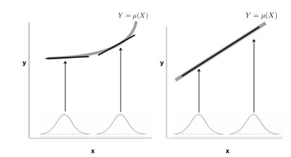
Figure 2: Dependence of the Population Best Linear Approximation on the Marginal Distribution of the Regressors

Ignoring the randomness of the regressors and their marginal distribution is perilous under misspecification. Figure 2 shows why. The left and right side pictures both compare the effects of different regressor distributions for a single regressor variable $X$ in two situations: misspecification and correct specification, respectively. The left plot shows a case of misspecification in which the true mean function $\mu(X)$ is nonlinear and yet, a linear function is fitted. The best linear approximation to the nonlinear mean function depends on the regressor distribution $\boldsymbol{P}_{\!\!\vec{\boldsymbol{X}}}$. Therefore, the “true parameters” $\boldsymbol{\beta}$ — the slope and intercept of the best fitting line at the population — will also depend on the regressor distribution. Specifically, one can see that for the left marginal distribution the intercept is larger and the slope is smaller than for the right marginal distribution. This implies that under misspecification the regressor distribution $\boldsymbol{P}_{\!\!\vec{\boldsymbol{X}}}$, thought of as a “non-parametric nuisance parameter,” is no longer ancillary.

The right side plot of Figure 2 shows a case of correct specification: The true mean function $\mu(X)$ (gray line) is linear. Consequently, the best linear approximation is trivially the same (black line) for both regressor distributions. In this case, the population marginal distribution of $X$ does not matter for the best linear approximation. There is one value for $\boldsymbol{\beta}$ no matter where the mass of $X$ falls. This makes the regressor distribution $\boldsymbol{P}_{\!\!\vec{\boldsymbol{X}}}$ ancillary for the parameters of the best linear fit.

The lessons from Figure 2 generalize to multiple linear regression with multivariate $\vec{\boldsymbol{X}}$, but the effects illustrated by the figure are magnified. Although one may argue that with a single regressor it should be easy to diagnose the misspecification, the challenges escalate for progressively larger numbers of regressors, and become nearly impossible in “modern” settings where the number of regressors exceeds the sample size, and data analysts tend to gamble on sparsity.

Practical implications and questions arise immediately. First, it is the combination of a misspecified working model and random regressors that produces the complications — it matters where the regressors fall. Second, one may wonder about the meaning of slopes when the model is not assumed to be correct. Third, what is the use of predicted values $\hat{y}=\vec{\boldsymbol{x}}^{\prime}\boldsymbol{\beta}$? Fourth, what form should statistical inference take when there is no reliance on the usual assumptions? Specifically, how are standard errors and associated $p$-values and confidence intervals affected by model misspecification? We will discuss possible answers to these questions in the remaining sections.

6 Conditional Mean Functions versus Regressor Distributions

The difficulties illustrated by Figure 2 suggests possibilities that may occur in various appplications, ranging from modeling of grouped data to meta-analysis. Consider the following hypothetical scenarios that should serve as cautions when interpreting models that are approximations. In Section 8 we will provide ways to interpret properly misspecified fitted linear functions.

Imagine a study of employed females and males in a certain industry, with income as response and a scale measuring education level as regressor. Consider next the possibility that there is one conditional mean function for income irrespective of gender, but the mean function may be nonlinear in the education scale, as illustrated by the left side picture in Figure 2. A data analyst may fit a linear model, perhaps because of convention, a high level of noise obscuring the nonlinearity, or a lack of graphical data exploration. The analyst may then find that different slopes are required for males and females and may respond by including in the regression an interaction term between gender and education. If, however, the truth is as stipulated, the usual interpretation of interaction effects would be misleading. The driver of the gender difference is not in how income responds to education, but the education scale distribution by gender. Put in different language, one may say that the real story is in the consequences of an association between gender and education.

Imagine now meta-analysis of randomized clinical trials (RCTs). RCTs often produce different apparent treatment effects for the same intervention, sometimes called “parameter heterogeneity.” Suppose the intervention is a subsidy for higher education, and the response is income at some defined end point. In two different locales, the average education levels may differ. Consequently, in each setting the intervention works off different baselines. There can be an appearance of different treatment effects even though the nonlinear mean returns to education may be the same in the both locales. The issue is, once again, that the difference in effects on returns to education may not derive from different conditional mean functions but from differences between regressor distributions.

Apparent parameter heterogeneity also can materialize in the choice of covariates. The coefficient $\beta_{1}$ of the regressor $X_{1}$ is not to be interpreted in isolation. $\beta_{1}$ depends on what other regressors are included. In the simplest case, a regression on $X_{1}$ alone, differs a regression on $X_{1}$ and $X_{2}$, Fitting a best approximation using $X_{1}$ alone produces a value of $\beta_{1}$ that would be the same in a regression on $X_{1}$ and $X_{2}$ if the two regressors were strictly uncorrelated. In observational data, $X_{1}$ and $X_{2}$ are likely to be partially collinear or “confounded” to various degrees. It matters for $\beta_{1}$ whether $X_{2}$ is included in the regression. In the extreme, the coefficients $\beta_{1}$ obtained from the two regressions may have different signs, suggesting an instance of Simpson’s paradox (see Berk et al. 2013, Section 2.1, for a more detailed discussion). For our discussion, exclusion versus inclusion of $X_{2}$ can be interpreted as a difference in regressor distributions, namely, that of the marginal distribution of $X_{1}$ compared to the bivariate distribution of $(X_{1},X_{2})$.

The prospect of more than one regressor can introduce further complications in practice. If some of the candidate regressors are unrelated to the response, variable selection procedures are sometimes employed. A common and heroic assumption is that the mean function is correctly specified save for some unnecessary regressors, and that such regressors can be found and discarded. Perhaps the most fundamental difficulty is how to formulate a proper estimand for different models defined by different subsets of the regressors when none of the models is correctly specified. For us, that the target of estimation is the best approximation at the population for the regressors selected. But within our approach, any approximation can be best by the least squares criterion, and the slopes of regressors included in more than one approximation can vary dramatically. One must also properly handle the post selection inference.

7 Estimation and Standard Errors

With i.i.d. multivariate data $(Y_{i},\vec{\boldsymbol{X}}_{i})$ ($i=1,\ldots,n$) from $\boldsymbol{P}$ on hand, one can apply OLS and obtain the plug-in estimate $\hat{\boldsymbol{\beta}}=\boldsymbol{\beta}(\hat{\boldsymbol{P}}_{\!n})$ derived from (1), where $\hat{\boldsymbol{P}}_{\!n}$ denotes the empirical distribution of the dataset. By multivariate central limit theorems, the regression estimates for the slopes of the best linear approximation in the OLS sense are asymptotically unbiased and normally distributed. These estimates are also asymptotically efficient in the sense of semi-parametric theory (e.g, Levit 1976, p. 725, ex. 5; Tsiatis, 2006, p. 8 and ch. 4).

7.1 Sandwich Standard Error Estimates

The asymptotic variances of the OLS regression estimates in the assumption lean i.i.d. sampling framework deviate from those of linear models theory which assumes linearity and homoskedasticity. The appropriate asymptotic variance is instead of a “sandwich” form (White, 1980a):

$$\boldsymbol{AV}[\boldsymbol{\beta},\boldsymbol{P}]=\boldsymbol{E}[\vec{\boldsymbol{X}}\vec{\boldsymbol{X}}^{\prime}]^{-1}\;\boldsymbol{E}[\delta^{2}\vec{\boldsymbol{X}}\vec{\boldsymbol{X}}^{\prime}]\;\boldsymbol{E}[\vec{\boldsymbol{X}}\vec{\boldsymbol{X}}^{\prime}]^{-1}.$$ (5)

A plug-in estimator is obtained as follows:

$$\widehat{\boldsymbol{AV}}=\boldsymbol{AV}[\hat{\boldsymbol{\beta}},\hat{\boldsymbol{P}}_{\!n}]=\left(\frac{1}{n}\sum_{i}\vec{\boldsymbol{X}}_{i}^{\prime}\vec{\boldsymbol{X}}_{i}\right)^{-1}\;\left(\frac{1}{n}\sum_{i}r_{i}^{2}\vec{\boldsymbol{X}}_{i}^{\prime}\vec{\boldsymbol{X}}_{i}\right)\;\left(\frac{1}{n}\sum_{i}\vec{\boldsymbol{X}}_{i}^{\prime}\vec{\boldsymbol{X}}_{i}\right)^{-1},$$ (6)

where $r_{i}=Y_{i}-\vec{\boldsymbol{X}}_{i}^{\prime}\hat{\boldsymbol{\beta}}$ are the sample residuals and $\hat{\boldsymbol{P}}_{\!n}$ is the empirical distribution of the data $(Y_{i},\vec{\boldsymbol{X}}_{i})$ $(i=1,...,n)$. Equation (6) is the simplest form of sandwich estimator of asymptotic variance. More refined forms exist but are outside the scope of this article. Standard error estimates for OLS regression coefficient estimates $\hat{\beta}_{j}$ are obtained from (6) using the asymptotic variance estimate in the $j$’th diagonal element:

$$S\!E_{j}=\left(\frac{1}{n}\widehat{\boldsymbol{AV}}_{\!j,j}\right)^{1/2}.$$

A connection with linear models theory is as follows. If the truth is linear and homoscedastic, hence the working model is correctly specified to first and second order, then the sandwich formula (5) collapses to the conventional formula for asymptotic variance due to $\boldsymbol{E}[\delta^{2}\vec{\boldsymbol{X}}\vec{\boldsymbol{X}}^{\prime}]=\sigma^{2}\boldsymbol{E}[\vec{\boldsymbol{X}}\vec{\boldsymbol{X}}^{\prime}]$, which in turn follows from $\boldsymbol{E}[\delta^{2}|\vec{\boldsymbol{X}}]=\boldsymbol{E}[\epsilon^{2}|\vec{\boldsymbol{X}}]=\sigma^{2}$. The result is $\boldsymbol{AV}[\boldsymbol{\beta},\boldsymbol{P}]=\sigma^{2}\boldsymbol{E}[\vec{\boldsymbol{X}}\vec{\boldsymbol{X}}^{\prime}]^{-1}$. This is the “assumption laden” form of asymptotic variance.

7.2 Bootstrap Standard Error Estimates

An alternative to standard error estimates based on the sandwich formula is obtained from the nonparametric pairwise or $x$-$y$ bootstrap which resamples tuples $(Y_{i},\vec{\boldsymbol{X}}_{i})$. It is transparently assumption lean in that it relies for asymptotic correctness essentially only on iid sampling of the tuples $(Y_{i},\vec{\boldsymbol{X}}_{i})$ and some technical moment conditions. The $x$-$y$ bootstrap therefore applies to all manners of regressions, including GLMs.

In stark contrast, the residual bootstrap is inappropriate. It necessarily assumes first order correctness, $\mu(\vec{\boldsymbol{x}})=\boldsymbol{\beta}^{\prime}\vec{\boldsymbol{x}}$, as well as homoskedastic population residuals $\delta$. The only step towards assumption leanness is a relaxation of Gaussianity of the error distribution. Furthermore, it does not apply to other forms of regression such as logistic regression. The residual bootstrap seems to be preferred by those who insist that one should condition on the regressors because they are ancillary. But as argued in Section 5, the ancillarity argument assumes correct specification of the linear regression model with independent errors, controverting the idea that models are approximations rather than truths.

Sandwich and bootstrap estimators of standard error are identical in the asymptotic limit, and on finite data they tend to be close. Based on either, one may perform conventional statistical tests and form confidence intervals. Although asymptotics are a justification for either, one of the advantages of the bootstrap is that it lends itself to a diagnostic to assessment of whether asymptotic normality is a reasonable assumption for the analysis being undertaken. One simply creates normal quantile plots of bootstrap estimates obtained in the requisite simulations. Finally, bootstrap confidence intervals have be addressed in extensive research showing that there are variants demonstably higher order correct. See, for example, Hall (1992), Efron and Tibshirani (1994), Davison and Hinkley (1997). An elaborate double-bootstrap procedure for regression is described in McCarthy et al. (2017).

8 Interpretations

8.1 Slopes from Best Approximations

When the estimation target is the best linear approximation, one can capitalize on desirable model-robust properties not available from assumption laden, linear models theory. The price is that subject-matter interpretations address features of the best linear approximation, not that of a “generative truth” — which, as we have emphasized, is often an unrealistic notion.

The most important interpretive issues are associated with the regression coefficients of the best linear approximation. The problem is that the standard interpretation of a regression coefficient is not strictly applicable anymore: It no longer holds that

• $\beta_{j}$ is the average difference in $Y$ for a unit difference in $X_{j}$ at constant levels of all other regressors $X_{k}$.

This statement uses the classical “ceteris paribus” (all things being equal) clause, which only holds when the response function is indeed linear. One gets closer to a generalizable interpretation if one modifies two details of this formulation as follows:

• $\beta_{j}$ is the average ratio of differences in $Y$ over differences in $X_{j}$, linearly adjusted for all other regressors $X_{k}$.

To give this interpretation precise meaning, we focus on the population target and consider for the moment a single regressor only. The slope of the simple regression through the origin of $Y$ on $X$ is then $\beta=\boldsymbol{E}[\,YX\,]/\boldsymbol{E}[\,X^{2}\,]$. It is a matter of elementary algebra to show that $\beta$ also equals the following suggestive expression:

$$\beta=\boldsymbol{E}[\,w(X\!-\!X^{\prime})\,\frac{Y\!-\!Y^{\prime}}{X\!-\!X^{\prime}}\,]~{}~{}~{}~{}\textrm{where}~{}~{}~{}~{}w(X\!-\!X^{\prime})=\frac{(X\!-\!X^{\prime})^{2}}{\boldsymbol{E}[\,(X-\!X^{\prime})^{2}\,]}.$$ (7)

Here $(X,Y)$ and $(X^{\prime},Y^{\prime})$ are two points drawn independently from the joint $(X,Y)$ distribution, hence $(Y\!-\!Y^{\prime})/(X\!-\!X^{\prime})$ is the slope of the line through this pair of points. Formula (7) says that these pairwise slopes average out to the slope $\beta$ of the OLS approximation when weighted proportionately to squared horizontal distances $(X\!-\!X^{\prime})^{2}$. These weights lend more influence to point pairs that are far from each other on the $X$-axis and are, therefore, more informative for the slope. Thus, $\beta$ is indeed a weighted average of pairwise slopes.

To extend the interpretation to more than one regressor, we only need to observe that the multiple regression coefficient $\beta_{j}$ is the simple regression coefficient through the origin with regard to $X_{j}$, linearly adjusted for all other regressors. The same interpretation is available for estimates $\hat{\beta}_{j}$ through its plug-in. In either case, formula (7) provides an interpretation of slopes as distance-weighted averages of pairwise slopes obtained from linearly adjusted regressors (see Buja et al. 2016a for more details).

8.2 Predicted Values $\hat{y}$ from Best Approximations

Also of interest are the predicted values at specific locations $\vec{\boldsymbol{x}}$ in regressor space, estimated as $\hat{y}_{\vec{\boldsymbol{x}}}=\hat{\boldsymbol{\beta}}^{\prime}\vec{\boldsymbol{x}}$. In linear models theory, for which the model is assumed correct, there is no bias if it is the true response surface that is estimated by predicted values. That is, $\boldsymbol{E}[\hat{y}_{\vec{\boldsymbol{x}}}]=\boldsymbol{\beta}^{\prime}\vec{\boldsymbol{x}}=\mu(\vec{\boldsymbol{x}})$ because $\boldsymbol{E}[\hat{\boldsymbol{\beta}}]=\boldsymbol{\beta}$, where $\boldsymbol{E}[\ldots]$ refers only to the randomness of the response values $y_{i}$ with the regressor vectors $\vec{\boldsymbol{X}}_{i}$ treated as fixed.

When the model is mean-misspecified such that $\mu(\vec{\boldsymbol{x}})\neq\boldsymbol{\beta}^{\prime}\vec{\boldsymbol{x}}$, then $\hat{y}_{\vec{\boldsymbol{x}}}$ is an estimate of the best linear approximation $\boldsymbol{\beta}^{\prime}\vec{\boldsymbol{x}}$, not $\mu(\vec{\boldsymbol{x}})$. Hence, there exists bias $\mu(\vec{\boldsymbol{x}})-\boldsymbol{\beta}^{\prime}\vec{\boldsymbol{x}}=\eta(\vec{\boldsymbol{x}})$ that does not disappear with increasing sample size $n$. Insisting on consistent prediction with linear equations at a specific location $\vec{\boldsymbol{x}}$ in regressor space is, therefore, impossible.

In order to give meaning to predicted values $\hat{y}_{\vec{\boldsymbol{x}}}$ under misspecification, it is necessary to focus on a population of future observations $(Y_{f},\vec{\boldsymbol{X}}_{f})$ and to assume that it follows the same joint distribution $\boldsymbol{P}_{\!\!Y,\vec{\boldsymbol{X}}}$ as the earlier training data $(Y_{i},\vec{\boldsymbol{X}}_{i})$. In particular, the future regressors are not fixed but random according to $\vec{\boldsymbol{X}}_{f}\sim\boldsymbol{P}_{\!\!\vec{\boldsymbol{X}}}$. If this is a reasonable assumption, then $\hat{y}_{\vec{\boldsymbol{X}}_{f}}$ is indeed the best linear prediction of $\mu(\vec{\boldsymbol{X}}_{f})$ and $Y_{f}$ for this future population under squared error loss. Averaged over future regressor vectors, there is no systematic bias because $\boldsymbol{E}[\eta(\vec{\boldsymbol{X}}_{f})]=0$ according to (4) of Section 4. Asymptotically correct prediction intervals for $Y_{f}$ do exist and, in fact, the usual intervals of the form

$$P\!I_{n}(\vec{\boldsymbol{x}};K)~{}:=~{}\left[\hat{y}_{\vec{\boldsymbol{x}}}\pm K\cdot\hat{\sigma}\cdot\left(1+\vec{\boldsymbol{x}}^{\prime}\left(\sum_{i=1\ldots n}\vec{\boldsymbol{X}}_{i}^{\prime}\vec{\boldsymbol{X}}_{i}\right)^{-1}\vec{\boldsymbol{x}}\right)\right]$$ (8)

can be used. However, the usual multiplier $K$ is based on linear models theory with fixed regressors. It is not robust to misspecification. There exists a simple alternative for choosing $K$ that has asymptotically correct predictive coverage under misspecification. It can be obtained by calibrating the multiplier $K_{n}$ empirically on the training sample such that the desired fraction $1-\alpha$ of observations $(Y_{i},\vec{\boldsymbol{X}}_{i})$ falls in their respective intervals. One estimates $\hat{K}_{n}$ by satisfying an approximate equality as follows, rounded to $\pm 1/n$:

$$\frac{1}{n}\cdot\#\left\{i\in\{1,\ldots,n\}:~{}Y_{i}\in P\!I(\vec{\boldsymbol{X}}_{i};\hat{K}_{n})\,\right\}~{}\approx~{}1-\alpha.$$

Under technical conditions, such multipliers will produce asymptotically correct prediction coverage:

$$\boldsymbol{P}\left[\,Y_{f}\in P\!I(\vec{\boldsymbol{X}}_{f};K_{n})\,\right]~{}\rightarrow~{}1-\alpha~{}~{}~{}\textrm{as}~{}~{}~{}n\rightarrow\infty,$$

where $\boldsymbol{P}[\ldots]$ accounts for randomness in the training data as well as the future data. (For more honest prediction, one might consider a cross-validated version of calibration based on repeatedly leaving out random portions of the data in fitting and estimating $\hat{K}_{n}$ from those portions.)

This method of calibration is certainly not unique for the prediction intervals of the form shown in (8). Its essential feature is that the intervals form a one-parameter nested family:  $P\!I_{n}(\vec{\boldsymbol{x}};K)\subset P\!I_{n}(\vec{\boldsymbol{x}};K^{\prime})$  for $K\leq K^{\prime}\in{\mathrm{I}\!\mathrm{R}}$. Thus, calibration for prediction can be applied to many other forms of nested intervals, but those of (8) are conventional and optimal under correct specification and yet, made asymptotically accurate under misspecification by the simple device of empirical calibration.

8.3 Causality and Best Approximation

Misspecification creates important challenges for causal inference. Consider first a randomized experiment with potential outcomes $Y_{1},Y_{0}$ for a binary treatment/intervention $C\in\{0,1\}$. Because of randomization, the potential outcomes are independent of the intervention: $(Y_{1},Y_{0})\perp\!\!\!\perp C$. Unbiased estimates of the Average Treatment Effect (ATE) follow. Pre-treatment covariates $\vec{\boldsymbol{X}}$ can be used to increase precision (reduce standard errors) only, similar to control variates in Monte Carlo (MC) experiments. It has been known for some time that the model including the treatment $C$ and the pre-treatment covariates $\vec{\boldsymbol{X}}$ does not need to be correctly specified to provide correct estimation of the ATE and (possibly) an asymptotic reduction of standard errors. That is, the model $Y\sim\tau C+\boldsymbol{\beta}^{\prime}\vec{\boldsymbol{X}}$ may be arbitrarily misspecified, and yet the ATE agrees with the treatment coefficient $\tau$. (To yield a benefit, however, the covariates $\vec{\boldsymbol{X}}$ must produce a useful increase in $R^{2}$ or some other appropriate measure of fit, similar to control variates in MC experiments.)

Now consider observational studies. There can be one or more variables that are thought of as causal and which can at least in principle be manipulated independently of the other covariates. If there is just one causal binary variable $C$, we are returned to a model of the form $Y\sim\tau C+\boldsymbol{\beta}^{\prime}\vec{\boldsymbol{X}}$, where it would be desirable for $\tau$ to be interpretable as an average treatment effect (Angrist and Pischke, 2009, Section 3.2). These are always very strong claims that often call for special scrutiny. It is widely known that causal inference properly can justified by assuming one of two sufficient conditions, known as “double robustness” (see, e.g, Bang and Robins 2005, Rotnitzki et al. 2012): (1) Either the mean function for $Y$ is correctly specified, which in practice means that there is no “omitted variables” problem for the response and that the functional form of the conditional mean function for $Y$ is correct; or (2) the conditional probability of treatment (called the propensity score) can be correctly modeled, which in practice means that there is no omitted variables problem for treatment probabilities and that the (usually logistic) functional form of the treatment probabilities is correct. In either case, omitted variable concerns are substantively characterized and not be satisfactorily addressed by formal statistical methods (Freedman, 2004). There are certainly diagnostic proposals based on proxies for potentially missing variables or based on instrumental variables, but the assumptions required a hardly lean. (see, for example, Hausman 1978). Misspecification of the functional form of the conditional response mean or the treatment probabilities are probably more appropriate for formal diagnostics.

In summary, causal inferences based observational data are fragile because they depend on two things: (1) correct model specification for at least one of two response variables, the response mean or the treatment probability, and (2) correctly deciding which one it is. Best approximation under misspecification won’t do. As a consequence, tremendous importance can fall to diagnostics of model fit. See Buja et al. (2016b) for some useful diagnostics that are applicable in all types of regressions for i.i.d. observations. But then, we are no longer doing assumption lean regression.

9 Generalizations

Focussing regression functionals provides possibilities for generalization. A first and readily apparent generalization is to statistical functionals other than slopes of the best linear approximation. Conditional variances come to mind. For example, if medical expenses are made a function of income, there can be more variation around the conditional mean for high-income households because they can afford more discretionary medical procedures.

A second and equally apparent generalization is to regressions other than linear OLS, such as generalized linear models and in particular, to linear logistic regression. The response is now binary, which suggests modeling conditional Bernoulli probabilities with a suitable link function and a cost function other than least squares. Interpreting the parameters as functionals allows the conditional distributions of the binary response to be largely arbitrary. One need not assume the logistic model is correct. The working model becomes a heuristic that produces a plausible cost function.

In detail, for a binary response $Y\in\{0,1\}$ one models the logit of the conditional probabilities

$$p(\vec{\boldsymbol{x}})~{}=~{}\boldsymbol{P}[Y\!=\!1|\vec{\boldsymbol{X}}\!=\!\vec{\boldsymbol{x}}]~{}=~{}\boldsymbol{E}[Y|\vec{\boldsymbol{X}}\!=\!\vec{\boldsymbol{x}}]$$

with a linear function of the regressors:

$$\mathrm{logit}(p(\vec{\boldsymbol{x}}))=\log(p(\vec{\boldsymbol{x}})/(1-p(\vec{\boldsymbol{x}})))~{}\approx~{}\boldsymbol{\beta}^{\prime}\vec{\boldsymbol{x}}.$$

The ${\rm logit}(p(\vec{\boldsymbol{x}}))$ maps in reverse to a model of the conditional probabilities via the sigmoid function that is the natural link function of the Bernoulli model:

$$p(\vec{\boldsymbol{x}})~{}\approx~{}\phi(\boldsymbol{\beta}^{\prime}\vec{\boldsymbol{x}}),~{}~{}\textrm{where}~{}~{}\phi(t)=\exp(t)/(1+\exp(t)).$$

In both cases, we use “$\approx$” rather than “$=$” to indicate the use of an approximation that allows varying degrees of misspecification.

The negative log-likelihood of the model when $n\rightarrow\infty$ results in a population cost function whose minimization produces the statistical functional (= estimand = “population parameter”) as follows:

$$\boldsymbol{\beta}(\boldsymbol{P})~{}:=~{}\operatorname*{argmin}_{\boldsymbol{\beta}\in{\mathrm{I}\!\mathrm{R}}^{p+1}}\boldsymbol{E}\left[\log\left(1+\exp\big{(}\vec{\boldsymbol{X}}^{\prime}\boldsymbol{\beta}\big{)}\right)-\big{(}\vec{\boldsymbol{X}}^{\prime}\boldsymbol{\beta}\big{)}\,Y\right].$$ (9)

The usual estimates $\hat{\boldsymbol{\beta}}$ are obtained by plug-in, replacing the expectation with the mean over the observations and thereby returning to the negative log-likelihood of the sample.

Interpretations and practice follow much as earlier, with the added complications caused by the nonlinear link function $\phi(t)$. The estimate $\hat{\boldsymbol{\beta}}$ correspond to a best approximiation $\phi(\boldsymbol{\beta}^{\prime}\vec{\boldsymbol{x}})$ of the true response surface $p(\vec{\boldsymbol{x}})$. The estimates $\hat{p}(\vec{\boldsymbol{x}})=\phi(\hat{\boldsymbol{\beta}}^{\prime}\vec{\boldsymbol{x}})$ are able to target only the best approximation $\phi(\boldsymbol{\beta}^{\prime}\vec{\boldsymbol{x}})$ where $\boldsymbol{\beta}=\boldsymbol{\beta}(\boldsymbol{P})$, not the true $p(\vec{\boldsymbol{x}})$. The approximation discrepancy $p(\vec{\boldsymbol{x}})-\phi(\boldsymbol{\beta}^{\prime}\vec{\boldsymbol{x}})$ does not vanish with more data, $n\rightarrow\infty$.

For standard errors, and statistical tests and confidence intervals based on them, one should use the appropriate sandwich estimators or standard error estimates obtained from the nonparametric $x$-$y$ bootstrap. Both have asymptotic justification under i.i.d. sampling of the tuples $(Y_{i},\vec{\boldsymbol{X}}_{i})$ for the best approximation target $\boldsymbol{\beta}(\boldsymbol{P})$.

Finally, under misspecification the regression functional $\boldsymbol{\beta}(\boldsymbol{P})$ will generally, as before, depend on the distribution regressor $\boldsymbol{P}_{\!\!\vec{\boldsymbol{X}}}$. The regressors cannot be treated as ancillary and not held fixed. The regression functional $\boldsymbol{\beta}(\boldsymbol{P})$ can have different values depending on where in the regressor space the data fall.

10 An Empirical Example Using Poisson Regression

In order to show the ease with which the functional view can be applied within the generalized linear model, we consider an application using Poisson regression. The estimand is a best log-linear approximation of the true response surface, not the true response surface itself.

The particular Poisson regression will be applied to data from a criminal justice agency. Here is some context. An important feature of an arrest is the charges that police choose to file. One crime event can lead to one charge or many. Each charge for which there is a guilty plea or guilty verdict will have sanctions specified by statute. For example, an aggravated robbery is defined by the use of a deadly weapon, or an object that appears to be a deadly weapon, to take property of value. If that weapon is a firearm, there can then be a charge of aggravated robbery and a second charge of illegal use of a firearm. There can be penalties for each. A greater number of charges can be used by prosecutors as plea bargaining chips and can place an offender at greater risk of sanction. In this illustration, we consider correlates of the number of charges against an offender filed by the police.

The dataset for our illustration contains 10,000 offenders arrested between 2007-2015 in a particular urban jurisdiction. The data are a random sample from over three hundred thousand offenders arrested in the jurisdiction during those years. This pool is sufficiently large to make an assumed infinite population and iid sampling good approximations. During that period, the governing statutes, administrative procedures, and mix of offenders were effectively unchanged – there is a form of criminal justice stationarity. We use as the response variable the number of charges associated with the most recent arrest. Several regressors are available, all thought to be related to the outcome. Many other relevant regressors are not available (e.g., the consequences of the crime for its victims).

The approximation adopted here is a Poisson regression. It is a working model about which we make no claim that it is correctly specified. Consequently, we forfeit any causal claims, and we are not proposing any of the regressors as manipulable interventions. Finally, our assumption lean framework does not require that the response follows a conditional Poisson distribution. One reason for violating Poissonness is that the binary events constituting the counts do not need to be independent. Indeed, independence would be unrealistic. If the crime is an armed robbery, for example, the offender would be charged with aggravated robbery and a weapons offense. Ordinarily, such dependence would be a concern.

The results of the Poisson regression are shown in Table 1. The columns contain, from left to right, the following quantities:

1. the name of the regressor variable,

2. the usual Poisson regression coefficient,

3. the conventional standard errors,

4. the associated p-values,

5. standard errors computed using a nonparametric $x$-$y$ bootstrap,

6. standard errors computed with the sandwich estimator, and

7. the associated sandwich p-values.

	Coeff	SE	p-value	Boot.SE	Sand.SE	Sand-p
(Intercept)	1.8802	0.0205	0.0000	0.0522	0.0526	0.0000
Age	-0.0147	0.0006	0.0000	0.0016	0.0016	0.0000
Male	0.0823	0.0127	0.0000	0.0284	0.0299	0.0058
Number of Priors	0.0031	0.0002	0.0000	0.0005	0.0005	0.0000
Number of Prior Sentences	0.0002	0.0016	0.8868	0.0040	0.0039	0.9519
Number of Drug Priors	-0.0138	0.0008	0.0000	0.0021	0.0020	0.0000
Age At First Charge	0.0028	0.0009	0.0012	0.0022	0.0021	0.1935

Table 1: Poisson Regression Results for The Number of Crime Charges (n=10,000)

Even though the model is likely misspecified by conventional standards for any number of reasons, the coefficient estimates for the population approximation are asymptotically unbiased for the population best approximation. In addition, asymptotic normality holds and can be leveraged to produce approximate confidence intervals and p-values based on sandwich or $x$-$y$ bootstrap estimators of standard error.

With 10,000 observations, the asymptotic results effectively apply. None of this would be true for inferences based on assumption-laden theories that assume the working model to be correct.

The marginal distribution of the response (number of charges) is skewed to the right: The mean number of charges range from 1 to 40, with a mean of 4.7, a standard deviation of 5.5. Most offenders have a relatively small number of charges, but a few offenders have many.

Table 1 shows that some of the bootstrap and sandwich standard errors are rather different from the conventional standard errors, indicating indirectly that the conditional Poisson model is misspecified (Buja et al. 2016a). Moreover, there is a reversal of the test’s conclusion for “Age at First Charge” (i.e., the earliest arrest that led to a charge as an adult). The null hypothesis is rejected with conventional standard errors but is not rejected with a bootstrap or sandwich standard error.

This correction is sensible because a natural expectation would have been that the slope of “Age At First Charge” should be negative, not positive. Typically individuals who have an early arrest and charge are more likely to commit crimes later on for which there can be multiple charges.

In the present Poisson model, exponentiated regression coefficients are multipliers of the charge counts. We interpret each regressor accordingly if the null hypothesis is rejected based on sandwich/bootstrap standard errors:

• Age: Starting at the top of Table 1, each additional year of age multiplies the average charge count by a factor of 0.98. Ten additional years of age reduces the count by a factor of 0.86. Older offenders have fewer charges perhaps because the crimes they tend to commit are different from the crimes younger offenders commit. For instance, the crimes of younger offenders may be more likely to be gang-related.

• Male: Men on the average have a greater number of charges than women. The multiplier is 1.08, which means that there is about a 8% average difference. Compared to a women at the women’s mean of 4.7 charges, a man would on the average have 5.1 charges, holding all other covariates constant.

• Number of Priors: To get the same 8% increase from the exponentiated regression coefficients for the number of all prior arrests takes an increment of about 25 priors. Such increments are common. About 25% of the offenders in the data are first offenders (i.e., no prior arrests), and another 30% have 25 or more prior arrests. A gap of 25 priors is common in these data.

• Number of Drug Priors: Offenders with a greater number of prior arrests for drug offenses on the average have fewer charges after controlling for the other covariates. Drug offenders often have a large number of such arrests, so the small coefficient of -0.0138 matters. For 20 additional prior drug arrests, the average charge count is multiplied by a factor of .76. A long history of drug abuse can be debilitating so that the crimes committed are far less likely to involve violence and often entail little more than drug possession.

In summary, offenders who are young males with many prior arrests not for drug possession, will on average have substantially more criminal charges. Such offenders perhaps are likely to be disproportionately arrested for crimes of violence in which other felonies are committed as well. Therefore, a larger number of charges would be expected.

What about causal inference? It makes little sense to envision manipulating any of the regressors with all other regressors fixed. The different measures of prior record and age at first arrest are in the past. Even if one could alter them, many other upstream regressors would be altered as well. Gender and age are inherent features of an offender. It also makes little sense to assume that all excluded regressors are independent of those that are included. For example, there is no measure of gang membership in the data. But even if gang membership were a regressor, one surely would not have exhausted the list of potential confounders.

If causal inference is off the table, what have we gained? For one thing, we acquired a general understanding of certain associations among variables of interest. In particular, it is instructive that the findings are largely consistent with past research. Note that we still care about the signs of the regression coefficients as indicators of the direction of association between the response and a regressor adjusted for the presence of the other regressors. What has changed is that the rigidity of interpretation based on correct model specification is abandoned and replaced by greater realism and skepticism about what a regression coefficient is able to convey.

As for predictive use of the regression, the results could in principle be applied in real settings to inform risk assessments in future cases. We qualify such use with the cautions of Section 8.2 according to which prediction covergance is for a population of future cases that behave like the past population, not any fixed location in regressor space. To this end, prediction intervals should be directly calibrated on the data, not based on model trusting theory. The widths of such intervals can inform users whether the model contains any actionable information at all.

We have seen indirect indications of model misspecification Traditional model-trusting standard errors differ from assumption lean sandwich and bootstrap standard errors. Because of model misspecification, it is likely that the parameters of the best fitting model depend on where in regressor space the mass of the $X$-distribution falls. This raises concerns about the performance of out-of-sample prediction. If the out-of-sample data are not derived from a source stochastically similar to that in the analyzed sample, then these predictions may be wildly inaccurate.

11 Conclusions

Treating models as best approximations should replace treating models as if there are correct. Best approximations proceed with a fixed model explicitly acknowledging approximation discrepancies, sometimes called “model bias,” which do not disappear with more data. The model bias, however, does not create an asymptotic bias in estimates of best approximations. Parameters of best approximations are estimated with bias that disappears at the usual rapid rate.

In regression, a fundamental feature of best approximations is that they depend on regressor distributions. It follows that one cannot condition on regressors and treat regressors as fixed. Regressor variability must be included in treatments of the sampling variability for any estimates. This can be achieved by using model robust standard error estimates in statistical tests and confidence intervals. Two choices are readily available: sandwich estimators and bootstrap-based estimators of standard errors. For the latter, a strong arguments favor the nonparametric $x$-$y$ bootstrap over the residual bootstrap, because conditioning on the regressors and treating them as fixed is incorrect when there is misspecification.

In this article, we also offered at least three ways in which best approximations can be informative in practice: (1) model parameters are re-interpreted as regression functionals, (2) predictions are for populations rather than at fixed regressor locations, and (3) there exist well-known connections between misspecification with causal inference.

In summary, it is easy to agree with G.E.P. Box’ famous dictum, but there are consequences affecting the mechanics of statistical inference and the interpretations of statistical estimates. Assume and proceed statistics does not suffice. Nor does hand waving.

References

Angrist, J.D. and Pischke. J.-S. (2009). Mostly Harmless Econometrics: An Empiricist’s Companion. Princeton University Press.

Benjamin, D. J., Berger, J. O., Johannesson, M., Nosek, B. A., Wagenmakers, E.–J., Berk, R., Bollen, K. A., Brembs, B., Brown, L., Camerer, C., Cesarini, D., Chambers, C. D., Clyde, M., Cook, T. D., De Boeck, P., Dienes, Z., Dreber, A., Easwaran, K., Efferson, C., Fehr, E., Fidler, F., Field, A. P., Forster, M., George, E. I., Gonzalez, R., Goodman, S., Green, E., Green, D. P., Greenwald, A., Hadfield, J. D., Hedges, L. V., Held, L., Ho, T.–H., Hoijtink, H., Jones, J. H., Hruschka, D. J., Imai, K., Imbens, G., Ioannidis, J. P. A., Jeon, M., Kirchler, M., Laibson, D., List, J., Little, R., Lupia, A., Machery, E., Maxwell, S. E., McCarthy, M., Moore, D., Morgan, S. L., Munafó, M., Nakagawa, S., Nyhan, B., Parker, T. H., Pericchi, L., Perugini, M., Rouder, J., Rousseau, J., Savalei, V., Schönbrodt, F. D., Sellke, T., Sinclair, B., Tingley, D., Van Zandt, T., Vazire, S., Watts, D. J., Winship, C., Wolpert, R. L., Xie, Y., Young, C., Zinman, J., and Johnson, V. E. (2017, in press). “Redefine Statistical Significance.” Nature Human Behavior.

Bang, H., and Robins, J.M. (2005) “Doubly Robust Estimation in Missing Data and Causal Inference,” Biometrics 61, 962–972.

Bachoc, F., Preinerstorfer, D., and Steinberger, L. (2017). “Uniformaly valid confidence intervals post-model-selection.” arXiv:1611.01043.

Berk, R.A., Brown, L., Buja, A., Zhang, K., and Zhao, L. (2013). “Valid Post-Selection Inference.” The Annals of Statistics 41(2): 802–837.

Berk, R.A. (2003) Regression Analysis: A Constructive Critique. Newbury Park, CA.: Sage.

Berk, R.A., Sorenson, S.B., and Barnes, G. (2016). “Forecasting Domestic Violence: A Machine Learning Approach to Help Inform Arraignment Decisions. Journal of Empirical legal Studies 31(1): 94–115.

Box, G.E.P. (1976). “Science and Statistics.” Journal of the American Statistical Association 71(356): 791–799.

Buja, A., Berk, R., Brown, L., George, E., Pitkin, E., Traskin, M., Zhan, K., and Zhao, L. (2016a). “Models as Approximations — Part I: A Conspiracy of Nonlinearity and Random Regressors in Linear Regression.” arXiv:1404.1578

Buja, A., Berk, R., Brown, L., George, E., Arun Kuman Kuchibhotla, and Zhao, L. (2016b). “Models as Approximations — Part II: A General Theory of Model-Robust Regression.” arXiv:1612.03257

Davison, A.C., and Hinkley, D.V. (1997). Bootstrap Methods and Their Application, Cambridge University Press.

Cox, D.R. (1995). “Discussion of Chatfield” (1995). Journal of the Royal Statistical Society, Series A 158 (3), 455–456.

Efron, B., and Tibshirani, R.J. (1994). An Introduction to the Bootstrap, Boca Raton, FL: CRC Press.

Fisher, R.A. (1924). “The Distribution of the Partial correlation Coefficient.” Metron 3: 329-332.

Freedman, D.A. (1981). “Bootstrapping Regression Models.” Annals of Statistics 9(6): 1218–1228.

Freedman, D.A. (2004). “Graphical Models for Causation and the Identification Problem.” Evaluation Review 28: 267–293.

Freedman, D.A. (2009). Statistical Models Cambridge, UK: Cambridge University Press.

Hall, P. (1992). The Bootstrap and Edgeworth Expansion. (Springer Series in Statistics) New York, NY: Springer Verlag.

Hausman, J. A. (1978). “Specification Tests in Econometrics.” Econometrica 46 (6): 1251-–1271.

Hong, L., Kuffner, T.A., and Martin R. (2016).“On Overfitting and Post-Selection Uncertainty Assessments.” Biometrika 103: 1–4.

Imbens, G.W., and Rubin, D.B., (2015). Causal Inference Statistics, Social, and Biomedical Sciences: An Introduction. Cambridge: Cambridge University Press.

Koenker, R. (2005). Quantile Regression Cambridge: Cambridge University Press.

Kuchibhotla, A.K., Brown L.D., Buja, A., George, E., Zhao, L. (2018). “A Model Free Perspective for Linear Regression: Uniform-in-model Bounds for Post Selection Inference.” arXiv:1802.05801

Leamer, E.E. (1978). Specification Searches: Ad Hoc Inference with Non-Experimental Data. New York, John Wiley.

Levit, B. Y. (1976). “On the efficiency of a class of non-parametric estimates.” Theory of Probability & Its Applications, 20(4):723–740.

McCarthy, D., Zhang, K., Berk, R.A., Brown, L., Buja, A., George, E., and Zhao, L.(2017). “Calibrated Percentile Double Bootstrap for Robust Linear Regression Inference.” Statistica Sinica, forthcoming

Rotnitzky, A., Lei, Q., Sued, M. and Robins, J. M. (2012). “Improved Double-Robust Estimation in Missing Data and Causal Inference Models,” Biometrika 99, 439–-456.

Rubin, D. B. (1986). “Which Ifs Have Causal Answers.” Journal of the American Statistical Association 81: 961–962.

Searle, S.R. (1970). Linear Models. New York: John Wiley.

Lee, J. D., Sun, D.L., Sun, Y., and Taylor, J.E. (2016). “Exact Post-Selection Inference, with Application to the Lasso.” The Annals of Statistics 44(3): 907–927.

Tsiatis, A.A. (2006). Semiparametric Theory and Missing Data. New York: Springer.

Wager, S., and Athey, S. (2017). “Estimation and Inference of Heterogeneous Treatment Effects using Random Forests.” Journal of the American Statistical Association, in press.

White, H. (1980a). “Using Least Squares to Approximate Unknown Regression Functions.” International Economic Review 21(1): 149–170.

White H. (1980b). “A Heteroskedasticity-Consistent Covariance Matrix and a Direct Test for Heteroskedasticity.” Econometrica, 48, 817–838.