Phase Transition to Large Scale Coherent Structures in Two-Dimensional Active Matter Turbulence

Abstract

The collective motion of microswimmers in suspensions induce patterns of vortices on scales that are much larger than the characteristic size of a microswimmer, attaining a state called bacterial turbulence. Hydrodynamic turbulence acts on even larger scales and is dominated by inertial transport of energy. Using an established modification of the Navier-Stokes equation that accounts for the small-scale forcing of hydrodynamic flow by microswimmers, we study the properties of a dense suspension of microswimmers in two dimensions, where the conservation of enstrophy can drive an inverse cascade through which energy is accumulated on the largest scales. We find that the dynamical and statistical properties of the flow show a sharp transition to the formation of vortices at the largest length scale. The results show that 2d bacterial and hydrodynamic turbulence are separated by a subcritical phase transition.

Thin layers of bacteria in their planctonic phase form structures that are reminiscent of jets and vortices in turbulent flows Dombrowski et al. (2004); Dunkel et al. (2013a); Gachelin et al. (2014). This state has been called “bacterial turbulence” Dombrowski et al. (2004) because of the shape and form of the patterns, and has been seen in many swimming microorganisms Dombrowski et al. (2004); Dunkel et al. (2013a); Gachelin et al. (2014) and active nematics Sanchez et al. (2012); Zhou et al. (2014); Giomi (2015). Bacterial turbulence usually appears on scales much smaller than those of hydrodynamic turbulence, with its inertial range dynamics and the characteristic energy cascades Frisch (1995). A measure of this separation is the Reynolds number, which is of order $10^{-4}-10^{-6}$ for an isolated swimmer in a fluid at rest Purcell (1977) and typically several tens of thousands in hydrodynamic turbulence. Recent studies of the rheology of bacterial suspensions have indicated, however, that the active motion of pusher-type bacteria can lower considerably the effective viscosity of the suspension Hatwalne et al. (2004); Liverpool and Marchetti (2006); Sokolov and Aranson (2009); Gachelin et al. (2013); López et al. (2015); Marchetti (2015), to the point where it approaches an active-matter induced “superfluid” phase where the energy input from active processes compensates viscous dissipation Cates et al. (2008); Giomi et al. (2010). In such a situation the collective action of microswimmers can produce a dynamics that may be influenced by the inertial terms. In two dimensions, a possible connection to hydrodynamic turbulence is particularly intriguing because the energy cascade proceeds from small to large scales and can result in an accumulation of energy at the largest scales admitted by the domain, thereby forming a so-called condensate Kraichnan (1967); Hossain et al. (1983); Smith and Yakhot (1993); Alexakis and Biferale (2018). If bacterial turbulence can couple to hydrodynamic turbulence, then the inverse cascade in 2d provides a mechanism by which even larger scales can be driven. We here discuss the conditions under which such a coupling between bacterial and hydrodynamic turbulence can occur.

A dense bacterial suspension consists of active swimmers in a solvent. It is generally described in terms of coupled equations for the flow velocity of the suspension and a polarization vector field that captures the coarse-grained dynamics of the microswimmers. In most previous studies the fluid flow was slaved to the swimmer dynamics, so that the equations focussed on the velocity or polarization of the swimmers Wensink et al. (2012); Srivastava et al. (2016); Putzig et al. (2016). Here, following recent work by Słomka and Dunkel  Słomka and Dunkel (2015, 2017a), we examine instead the effective equation for the fluid flow, obtained by slaving the swimmer velocity to the velocity of the suspension Linkmann et al. (2019). Both approaches incorporate activity via active stresses that provide a forcing in the dynamical equations and yield minimal models that capture the pattern-formation process associated with bacterial turbulence Wensink et al. (2012); Słomka and Dunkel (2015). The effective Navier-Stokes equation for the fluid introduced in Refs. Słomka and Dunkel (2015, 2017a) bears a strong similarity to models studied in the context of inertial turbulence Beresnev and Nikolaevskiy (1993); Tribelsky and Tsuboi (1996), hence providing an excellent starting point for examining the relation between bacterial and hydrodynamic turbulence.

These effective models have been compared with experiments in Bacillus subtilis Wensink et al. (2012); Dunkel et al. (2013a); Słomka and Dunkel (2017a), and have been widely used for investigating active turbulence Dunkel et al. (2013b); Bratanov et al. (2015); Słomka and Dunkel (2015); Srivastava et al. (2016); Putzig et al. (2016); Słomka and Dunkel (2017a, b); Doostmohammadi et al. (2017); James et al. (2018); Słomka et al. (2018). In this Letter we study the connection between 2d bacterial and hydrodynamic turbulence systematically within a model that focusses on the suspension flow and is, in that sense, independent of details of the bacterial motion. We use the model of Refs. Słomka and Dunkel (2015, 2017a), and slightly modify its structure so that that we have a single parameter that controls the strength of the bacterial forcing. Increasing this parameter, we find a discontinuous transition to flow states which are hydrodynamically turbulent in the strict sense, that is, they display an inverse energy cascade characterized by a scale-independent energy flux Kraichnan (1967); Frisch (1995); Boffetta and Ecke (2012).

For the model Słomka and Dunkel (2015, 2017a, 2017b), we take the velocity field $\bm{u}$ to be incompressible, $\nabla\cdot\bm{u}=0,$ and periodic in a rectangular domain. The momentum balance is Navier-Stokes like (with the density scaled to 1),

$$\partial_{t}\bm{u}+(\bm{u}\cdot\nabla)\bm{u}+\nabla p=\nabla\cdot{\bm{\sigma}}\ ,$$ (1)

where $p$ is the pressure and ${\bm{\sigma}}$ the stress tensor. The stress tensor contains three adjustable parameters $\Gamma_{i}$,

$$\sigma_{ij}=\left(\Gamma_{0}-\Gamma_{2}\Delta+\Gamma_{4}\Delta^{2}\right)\left(\partial_{i}u_{j}+\partial_{j}u_{i}\right)\ ,$$ (2)

and is most conveniently discussed in Fourier space, where the dissipative term in Eq. (1) can be used to introduce an effective viscosity, $\nabla\cdot{\bm{\sigma}}=\nu_{\rm eff}\Delta\bm{u}$, with

$$\tilde{\nu}_{\rm eff}(k)=\Gamma_{0}+\Gamma_{2}k^{2}+\Gamma_{4}k^{4}\ ,$$ (3)

where $\tilde{\nu}_{\rm eff}$ is the Fourier transform of $\nu_{\rm eff}$. The first parameter $\Gamma_{0}$ corresponds to the kinematic viscosity, and $\Gamma_{4}>0$ ensures that modes with large $k$ are always damped by hyperviscosity. If $\Gamma_{2}<0$ and sufficiently negative, the effective viscosity becomes negative in a range of wave numbers, thus providing a source of energy and instability. This is the only forcing in the model, it corresponds to the mesoscale vortices observed in bacterial turbulence, and without it all fields decay. In 2d and for a suitable set of parameters statistically stationary states with an inverse energy transfer from the band of forced wave numbers to smaller wave numbers have been found in variants of both minimal models Słomka and Dunkel (2015); Oza et al. (2016); Mickelin et al. (2018). The energy spectrum in Ref. Słomka and Dunkel (2015) showed a scaling exponent close to the Kolmogorov value of $-5/3$, characteristic of the constant-flux inverse energy cascade in 2d turbulence Boffetta and Ecke (2012). Small condensates were observed in Refs. Oza et al. (2016); Mickelin et al. (2018).

In the stress model given by Eq. (3) $\Gamma_{2}$ determines not only the strength but also the range of wave numbers that are forced. In order to eliminate this influence, we introduce a variant of the model, where the bacterial forcing is modeled by a piecewise constant viscosity (PCV) in Fourier space. We take

$$\tilde{\nu}(k)=\begin{cases}\nu_{0}>0\quad\text{for}\quad k<k_{\rm min}\ ,\\ \nu_{1}<0\quad\text{for}\quad k_{\rm min}\leqslant k\leqslant k_{\rm max}\ ,\\ \nu_{2}>0\quad\text{for}\quad k>k_{\rm max}\ .\end{cases}$$ (4)

where $\nu_{0}$, like $\Gamma_{0}$, is the kinematic viscosity of the suspension and $\nu_{1}$ and $\nu_{2}>\nu_{0}$ correspond to higher-order terms $\Gamma_{2}k^{2}$ and $\Gamma_{4}k^{4}$, respectively, in the gradient expansion of the active stresses in Eq. (3). That is, as in the model of Refs. Słomka and Dunkel (2017a, 2015), they arise from a linear relation between the suspension flow and the bacterial forcing. The latter is justified for dense 2d suspensions, where both polarization and suspension velocity are solenoidal, through a reduction in degrees of freedom Linkmann et al. (2019). With this model, the forced wavenumbers are confined to the interval $[k_{\rm min},k_{\rm max}]$ and the strength of the forcing is controlled by $\nu_{1}<0$. In what follows we carry out a parameter study of the PCV model where $\nu_{1}$ is the only variable parameter.

We solve the 2d PCV model in vorticity formulation

$$\partial_{t}\tilde{\omega}(\bm{k})+\mathcal{F}_{\bm{k}}{\left[\bm{u}\cdot\nabla\omega\right]}=-\tilde{\nu}(k)k^{2}\tilde{\omega}(\bm{k})\ ,$$ (5)

where $\omega$ is the vorticity, $\omega(x_{1},x_{2})\bm{e}_{3}=\nabla\times\bm{u}(x_{1},x_{2})$, and $\tilde{\cdot}\equiv\mathcal{F}_{\bm{k}}[\cdot]$ denotes the Fourier transform. The equations are integrated in Fourier space, in a domain $[0,2\pi]^{2}$ with periodic boundary conditions, and using the standard pseudospectral method with full dealiasing according to the 2/3rds rule Orszag (1971). The simulations are run without additional large-scale dissipation terms, until a statistically stationary state is reached. As this can take a long time, we used a resolution of $256^{2}$ collocation points to explore the parameter space, and confirmed the results for a few isolated parameter values with higher resolution, see Table 1. Different resolutions can be mapped onto each other using the invariance of Eq. (5) under the transformation

$$x\to\lambda x,\ \ t\to t,\ \ \nu\to\lambda^{2}\nu,\ \ \bm{u}\to\lambda\bm{u},\ \ \omega\to\omega.$$ (6)

For all simulations the initial data are Gaussian-distributed random velocity fields.

$N$	$|\nu_{1}/\nu_{0}|$	$\nu_{2}/\nu_{0}$	$k_{\rm min}$	$k_{\rm max}$	Re	$U$	$L$
256	0.25-7.0	10.0	33	40	19-13677	0.29-7.77	0.07-1.92
1024	1.0	10.0	129	160	45	0.027	0.029
1024	2.0	10.0	129	160	226	0.041	0.094
1024	5.0	10.0	129	160	132914	1.17	1.93

Table 1: Parameters used in DNSs of the piecewise constant viscosity model and resulting observables. The number of grid points in each coordinate is denoted by $N$, the viscosity $\nu_{0}$ and $\nu_{1}$, $\nu_{2}$, $k_{\rm min}$, $k_{\rm max}$ are the parameters in Eq. (4). The Reynolds number ${\rm Re}=UL/\nu_{0}$ is based on $\nu_{0}$, the root-mean-square velocity $U$ and the integral length scale $L=2/U^{2}\int_{0}^{\infty}dk\ E(k)/k$, with $\nu_{0}=1.1\times 10^{-3}$ for $N=256$ and $\nu_{0}=1.7\times 10^{-5}$ for $N=1024$. Averages in the statistically stationary state are computed from at least 1800 snapshots separated by one large-eddy turnover time $T=L/U$.

A measure of the formation of large scale structures is the energy at the largest scale, $E_{1}\equiv E(k=1)$, where

$$E(k)\equiv\left\langle\frac{1}{2}\int d\hat{\bm{k}}\ |\tilde{\bm{u}}(\bm{k})|^{2}\right\rangle_{t}\ ,$$ (7)

with $\hat{\bm{k}}=\bm{k}/|\bm{k}|$ a unit vector, is the time-averaged energy spectrum after reaching a statistically steady state. $E_{1}$ is shown as a function of the ratio $|\nu_{1}/\nu_{0}|$ in Fig. 1, together with typical examples of velocity fields. At low values $|\nu_{1}/\nu_{0}|\leqslant 2$ the energy at the largest scale is negligible and the corresponding flows at $|\nu_{1}/\nu_{0}|=2$ and $|\nu_{1}/\nu_{0}|=1$ do not show any large-scale structure. At a critical value $|\nu_{1,\rm crit}/\nu_{0}|=2.06\pm 0.02$ a sharp transition occurs so that for larger values of $|\nu_{1}/\nu_{0}|$ a condensate consisting of two counter-rotating vortices at the largest scales exists (see the case $|\nu_{1}/\nu_{0}|=5$ in Fig. 1, and Refs. Chertkov et al. (2007); Xia et al. (2009); Laurie et al. (2014)). Since a condensate can only build up once the transfer of kinetic energy reaches up to the largest scales, the presence of a condensate is a tell-tale sign of an inverse energy transfer.

For $|\nu_{1}|\gg|\nu_{1,\rm crit}|$, we observe $E_{1}\sim\nu_{1}^{2}$, which can be rationalized by mapping the large-scale dynamics onto an Ornstein-Uhlenbeck process Uhlenbeck and Ornstein (1930); Chandrasekhar (1943); Risken and Frank (1996); van Kampen (2007). Neglecting small-scale dissipation, Eq. (5) can formally be written as $\partial_{t}\omega=-\nu_{0}\Delta\omega_{\rm LS}-\nu_{1}\Delta\omega_{\rm IN}$, where $\omega_{\rm LS}$ and $\omega_{\rm IN}$ are the vorticity field fluctuations at scales larger and smaller than $\pi/k_{\rm min}$, respectively. For $\omega_{\rm LS}$, this results in an Ornstein-Uhlenbeck process with relaxation time $1/\nu_{0}$ and diffusion coefficient $\nu_{1}^{2}/2$, because $\omega_{\rm IN}$ can be considered as noise on the time-scale of $\omega_{\rm LS}$. Therefore, $E_{1}\simeq E_{\rm LS}\sim\nu_{1}^{2}/\nu_{0}$.

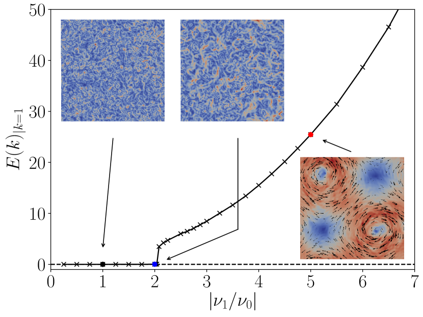
Figure 1: (Color online) Mean energy at the largest scale as a function of $\nu_{1}$. The black, blue and red dots correspond to cases $|\nu_{1}/\nu_{0}|=1$ , $|\nu_{1}/\nu_{0}|=2$ and $|\nu_{1}/\nu_{0}|=5$, respectively, and the corresponding visualisations show $|\bm{u}(\bm{x})|$.

The transition and its precursors can be analyzed in terms of energy spectra, shown in the top panel of Fig. 2 for three typical examples. As expected from the large-scale pattern observed for the case $|\nu_{1}/\nu_{0}|=5$, the corresponding energy spectrum shows the condensate as a high energy density at $k=1$. In the other two cases, $|\nu_{1}/\nu_{0}|=1$ and $|\nu_{1}/\nu_{0}|=2$, the energy density tapers off towards small wave numbers, and there is no condensate. The spectra for $k\leq k_{\rm min}$ follow power laws, with exponents in the range set by energy equipartion where $E(k)\sim k$, and a Kolmogorov scaling, $E(k)\sim k^{-5/3}$, as indicated by the solid lines in the figure. The spectral exponent is known to depend on large-scale dissipation, if present Bratanov et al. (2015), and on the presence of a condensate Chertkov et al. (2007). For the case $|\nu_{1}/\nu_{0}|=1$, the energy spectrum is $E(k)\sim k^{0.75}$, and close to the equipartition case. With increasing amplification factor the spectral exponent turns negative, with $E(k)\sim k^{-0.75}$ for $|\nu_{1}/\nu_{0}|=2$ and $E(k)\sim k^{-1.2}$ for $|\nu_{1}/\nu_{0}|=5$.

The occurrence of states close to absolute equilibrium in the region $k<k_{\rm min}$ for weak forcing suggests the presence of a second transition to a net inverse energy transfer for stronger forcing, as in the case $|\nu_{1}/\nu_{0}|=2$. Although the spectral exponent in this case suggests that energy is transferred upscale, the absence of a condensate implies that this energy transfer must stop before reaching $k=1$. The flux of energy across scale $k$ in the statistically steady state can be measured with

$$\Pi(k)\equiv-\left\langle\int_{|\bm{k}^{\prime}|\leq k}d\bm{k}^{\prime}\ \tilde{\bm{u}}(-\bm{k}^{\prime})\cdot\mathcal{F}_{\bm{k}^{\prime}}{\left[(\bm{u}\cdot\nabla)\bm{u}\right]}\right\rangle_{t}.\$$ (8)

The sign of $\Pi(k)$ is defined such that $\Pi(k)<0$ corresponds to an inverse energy transfer and $\Pi(k)>0$ to a direct energy transfer. As shown in Fig. 2, bottom panel, the fluxes tend to zero as $k$ tends to $1$ for $|\nu_{1}/\nu_{0}|=1$ and $|\nu_{1}/\nu_{0}|=2$, indicating that the inverse energy transfer is suppressed by viscous dissipation close to $k_{\rm min}$. In contrast, for $|\nu_{1}/\nu_{0}|=5$, the flux $\Pi(k)\simeq\rm const.$, clearly indicating an inertial range and hence an inverse energy cascade in the strict sense, as expected for a hydrodynamic energy transfer that is dominated by the inertial term in the Navier-Stokes equations.

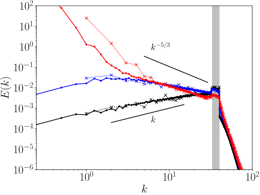
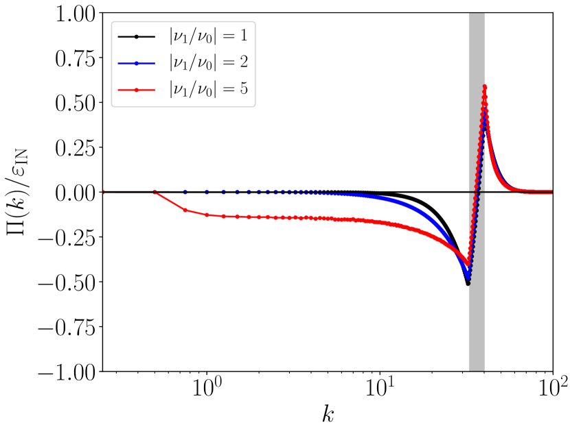
Figure 2: (Color online) Energy spectra (top) and fluxes (bottom) for three example cases $|\nu_{1}/\nu_{0}|=1$ (black) , $|\nu_{1}/\nu_{0}|=2$ (blue) and $|\nu_{1}/\nu_{0}|=5$ (red) for $N=256$ (dotted lines) and $N=1024$ (solid lines). The higher-resolved data has been rescaled according to Eq. (6) to account for $k\to 4k$. The gray-shaded area indicates the interval $[k_{\rm min},k_{\rm max}]$, and the solid lines in the top panel correspond to theoretical predictions, i.e. energy equipartion: $E(k)\sim k$, and Kolmogorov scaling: $E(k)\sim k^{-5/3}$.

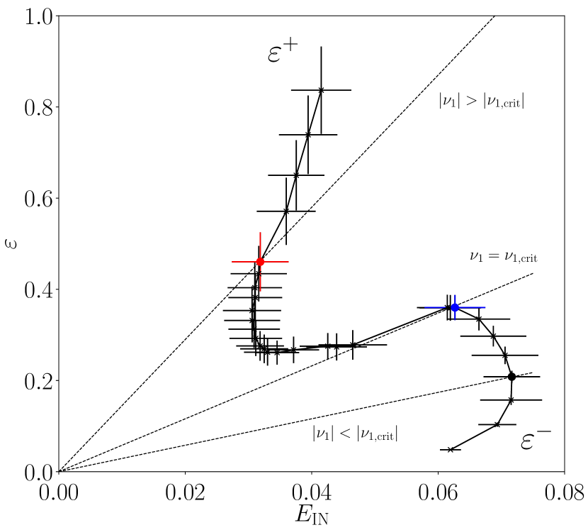
Figure 3: (Color online) Total mean dissipation rate as a function of the energy in the interval $[k_{\rm min},k_{\rm max}]$. The dashed lines indicate different values of the amplification factor. Error bars indicate the standard deviation. The larger open symbols in black, blue and red correspond to cases $|\nu_{1}/\nu_{0}|=1$, $|\nu_{1}/\nu_{0}|=2$ and $|\nu_{1}/\nu_{0}|=5$, respectively.

The transition shows up not only in the energy transfer across scales, but also in the total energy balance. The special form of Eq. (1) with the piecewise constant viscosity as in Eq. (4) gives a balance between the energy contained in the forced modes, $E_{\rm IN}\equiv\int_{k_{\rm min}}^{k_{\rm max}}dk\ E(k)$, and the dissipation in the other wave number regions, $\varepsilon=2\nu_{0}\int_{0}^{k_{\rm min}}dk\ k^{2}E(k)+2\nu_{2}\int_{k_{\rm max}}^{\infty}dk\ k^{2}E(k)$. In a statistically stationary state $\varepsilon\simeq 2k_{\rm f}^{2}|\nu_{1}|E_{\rm IN}$, where $k_{\rm f}=(k_{\rm min}+k_{\rm max})/2$ corresponds to an effective driving scale. Figure 3 presents the relation between $\varepsilon$ and $E_{\rm IN}$, obtained from simulations for different $\nu_{1}$. Statistically stationary states are obtained as crossings between $\varepsilon(E_{\rm IN})$ (the symbols connected by continuous lines) and the equilibrium condition $\varepsilon\simeq 2k_{\rm f}^{2}|\nu_{1}|E_{\rm IN}$, shown by dashed lines for different $\nu_{1}$.

For small $|\nu_{1}|$ the energy content in the forced wave number range increases with $|\nu_{1}|$. However, as the transfer to a wider range of wave numbers sets in dissipation increases, and the energy $E_{\rm IN}$ decreases (branch labelled $\varepsilon^{-}$). This is a smooth transition from absolute equilibrium to viscously damped inverse energy transfer. At the critical forcing $|\nu_{1,crit}|$, both $\varepsilon$ and $E_{\rm IN}$ drop, and a gap forms: the signal of the first-order phase transition. Further increasing $|\nu_{1}|$ results in even lower $E_{\rm IN}$, with only small variations in $\varepsilon$, so that $E_{\rm IN}\sim|\nu_{1}|^{-1}$. In this region, the dynamics cannot be dominated by the condensate. Eventually, the condensate takes over the energy dissipation; the curve turns around to give $\varepsilon\propto E_{1}\propto|\nu_{1}|^{2}$ and $E_{\rm IN}\propto\varepsilon^{1/2}$ (branch labelled $\varepsilon^{+}$). In this region, a strong condensate will alter the nonlinear dynamics Chertkov et al. (2007); Laurie et al. (2014) and the characteristic Kolmogorov scaling of $E(k)$ for 2d turbulence disappears. Finally, the particular S-shape of the curve shows that two non-equilibrium steady states corresponding to the branches $\varepsilon^{+}$ and $\varepsilon^{-}$, respectively, can be realised for the same value of the energy $E_{\rm IN}$ in the forced range. The existence of two stable branches connected by an unstable region describes the bistable scenario characteristic of a first-order non-equilibrium phase transition.

In order to relate the numerical data to experimental results, we now compare the Reynolds numbers and characteristic scales involved in active suspensions and in our simulations. For a suspension of B. subtilis, the characteristic size of the generated vortices is about $100\mu m$ with a characteristic velocity around $35-100\mu m$ Dombrowski et al. (2004), resulting in ${\rm Re}_{\rm vortex}=O(10^{-2}-10^{-3})$. Taking into account a possible reduction in viscosity down to a ‘superfluid’ regime measured experimentally for Escherichia coli López et al. (2015), a Reynolds number regime of $O(10)$ seems possible, provided the density of the suspension is not too high. Larger microswimmers may lead to even higher Reynolds numbers, with values of around 30 for magnetic spinners accompanied by Kolmogorov scaling of $E(k)$ Kokot et al. (2017), and 25 for camphor boats (C. Cottin-Bizonne, private communication).

The forcing in our equations models the scale of such vortices, so we need a corresponding Reynolds number for the comparison between the model and potential realizations. With $k_{\rm f}=(k_{\rm min}+k_{\rm max})/2$ the center of the forced modes, and $E_{\rm IN}$ the energy in these modes, we can define ${\rm Re}_{\rm B}=\sqrt{E_{\rm IN}}(\pi/k_{\rm f})/\nu_{0}$. Just above the critical point, we measure ${\rm Re}_{\rm B}\simeq 15$. While these value are still larger than the typical Reynolds number of active suspensions, an experimental realization of the transition seems within reach.

This comparison also gives relations for the length and time scales. Setting the forcing scale to $\pi/k_{\rm f}=50\mu m$, the lattice with $256^{2}$ collocation points corresponds to a box length of $3600\mu m$, larger than the usual experimental domain sizes. It is possible to detect the formation of the vortices also in smaller domains, but then it will be difficult to extract scaling exponents for the energy densities and the energy flux. For the time scales, the comparison is more favorable, with the large-eddy turnover time $T$ and the characteristic timescale of the mesoscale vortices $L_{\rm box}/\sqrt{E_{\rm IN}}$ resulting in $0.4s\leqslant T\leqslant 0.8s$, and hence a run time of $20-40min$ for the different simulations. For comparison, constant levels of activity in E. coli can be maintained for several hours López et al. (2015).

The systematic parameter study of a hydrodynamic model applicable to dense suspensions of microswimmers presented here shows a sharp transition between spatio-temporal chaos (bacterial turbulence) and large-scale coherent structures (hydrodynamic turbulence). The transition is preceded by a statistically steady state in which a net inverse energy transfer is damped by viscous dissipation at intermediate scales before reaching the largest scales in the system. Above the critical point, a condensate forms at the largest scales and the energy flux is scale-independent over a range of scales, i.e., the flows in that parameter range are hydrodynamically turbulent. A comparison between the driving-scale Reynolds number in our simulations and typical Reynolds numbers of active suspensions suggests that it should be possible to observe the transition to large scale coherent structures also experimentally. Our results should be generic for active systems where the forcing is due to linear amplification. For instance, we verified that also in the continuum model (Eq. (3)) the condensate forms suddenly under small changes in forcing at similar Reynolds numbers as in the PCV model Linkmann et al. (2019).

Finally, we note that in rotating Newtonian fluids, transitions to condensate states have been observed as a function of the rotation rate (Rossby number) Alexakis (2015); Yokoyama and Takaoka (2017); Seshasayanan and Alexakis (2018). This suggests that the appearance of a condensate may be connected with a phase transition also in other flows.

GB acknowledges financial support by the Departments of Excellence Grant (MIUR). MCM was supported by the National Science Foundation through Grant DMR-1609208.

References

- Dombrowski et al. (2004) C. Dombrowski, L. Cisneros, S. Chatkaew, R. E. Goldstein, and J. O. Kessler, Phys. Rev. Lett. 93, 098103 (2004).
- Dunkel et al. (2013a) J. Dunkel, S. Heidenreich, K. Drescher, H. H. Wensink, M. Bär, and R. E. Goldstein, Phys. Rev. Lett. 110, 228102 (2013a).
- Gachelin et al. (2014) J. Gachelin, A. Rousselet, A. Lindner, and E. Clement, New Journal of Physics 16, 025003 (2014).
- Sanchez et al. (2012) T. Sanchez, D. N. Chen, S. J. DeCamp, M. Heymann, and Z. Dogic, Nature 491, 431 (2012).
- Zhou et al. (2014) S. Zhou, A. Sokolov, O. D. Lavrentovich, and I. S. Aranson, Proc. Natl. Acad. Sci. U.S.A. 111, 1265 (2014).
- Giomi (2015) L. Giomi, Phys. Rev. X 5, 031003 (2015).
- Frisch (1995) U. Frisch, Turbulence: the legacy of A. N. Kolmogorov (Cambridge University Press, 1995).
- Purcell (1977) E. M. Purcell, Am. J. Phys. 45, 3 (1977).
- Hatwalne et al. (2004) Y. Hatwalne, S. Ramaswamy, M. Rao, and R. A. Simha, Phys. Rev. Lett. 92, 118101 (2004).
- Liverpool and Marchetti (2006) T. B. Liverpool and M. C. Marchetti, Phys. Rev. Lett. 97, 268101 (2006).
- Sokolov and Aranson (2009) A. Sokolov and I. S. Aranson, Phys. Rev. Lett. 103, 148101 (2009).
- Gachelin et al. (2013) J. Gachelin, G. Miño, H. Berthet, A. Lindner, A. Rousselet, and E. Clément, Phys. Rev. Lett. 110, 268103 (2013).
- López et al. (2015) H. M. López, J. Gachelin, C. Douarche, H. Auradou, and E. Clément, Phys. Rev. Lett. 115, 028301 (2015).
- Marchetti (2015) M. C. Marchetti, Nature Viewpoint 525, 37 (2015).
- Cates et al. (2008) M. E. Cates, S. M. Fielding, D. Marenduzzo, E. Orlandini, and J. Yeomans, Phys. Rev. Lett. 101, 068102 (2008).
- Giomi et al. (2010) L. Giomi, T. B. Liverpool, and M. C. Marchetti, Phys. Rev. E 81, 051908 (2010).
- Kraichnan (1967) R. H. Kraichnan, Phys. Fluids 10, 1417 (1967).
- Hossain et al. (1983) M. Hossain, W. H. Matthaeus, and D. Montgomery, J. Plasma Phys. 30, 479–493 (1983).
- Smith and Yakhot (1993) L. M. Smith and V. Yakhot, Phys. Rev. Lett. 71, 352 (1993).
- Alexakis and Biferale (2018) A. Alexakis and L. Biferale, Phys. Reports 767-769, 1 (2018).
- Wensink et al. (2012) H. H. Wensink, J. Dunkel, S. Heidenreich, K. Drescher, R. E. Goldstein, H. Löwen, and J. M. Yeomans, Proc. Natl. Acad. Sci. 109, 14308 (2012).
- Srivastava et al. (2016) P. Srivastava, P. Mishra, and M. C. Marchetti, Soft Matter 12, 8214 (2016).
- Putzig et al. (2016) E. Putzig, G. S. Redner, A. Baskaran, and A. Baskaran, Soft Matter 12, 3854 (2016).
- Słomka and Dunkel (2015) J. Słomka and J. Dunkel, Eur. Phys. J. Spec. Top. 224, 1349 (2015).
- Słomka and Dunkel (2017a) J. Słomka and J. Dunkel, Proc. Natl. Acad. Sci. 114, 2119 (2017a).
- Linkmann et al. (2019) M. Linkmann, M. C. Marchetti, G. Boffetta, and B. Eckhardt, arXiv:1905.06267 (2019).
- Beresnev and Nikolaevskiy (1993) I. A. Beresnev and V. N. Nikolaevskiy, Physica D 66, 1 (1993).
- Tribelsky and Tsuboi (1996) M. I. Tribelsky and K. Tsuboi, Phys. Rev. Lett. 76, 1631 (1996).
- Dunkel et al. (2013b) J. Dunkel, S. Heidenreich, M. Bär, and R. E. Goldstein, New J. Phys. 15, 045016 (2013b).
- Bratanov et al. (2015) V. Bratanov, F. Jenko, and E. Frey, Proc. Natl. Acad. Sci. 112, 15048 (2015).
- Słomka and Dunkel (2017b) J. Słomka and J. Dunkel, Phys. Rev. Fluids 2, 043102 (2017b).
- Doostmohammadi et al. (2017) A. Doostmohammadi, T. N. Shendruk, K. Thijssen, and J. M. Yeomans, Nature Comm. 8, 15326 (2017).
- James et al. (2018) M. James, W. J. T. Bos, and M. Wilczek, Phys. Rev. Fluids 3, 061101(R) (2018).
- Słomka et al. (2018) J. Słomka, P. Suwara, and J. Dunkel, J. Fluid Mech. 841, 702 (2018).
- Boffetta and Ecke (2012) G. Boffetta and R. E. Ecke, Annu. Rev. Fluid Mech. 44, 427 (2012).
- Oza et al. (2016) A. Oza, S. Heidenreich, and J. Dunkel, Eur. J. Phys. E 39, 97 (2016).
- Mickelin et al. (2018) O. Mickelin, J. Słomka, K. J. Burns, D. Lecoanet, G. M. Vasil, L. M. Faria, and J. Dunkel, Phys. Rev. Lett. 120, 164503 (2018).
- Orszag (1971) S. A. Orszag, J. Atmos. Sci. 28, 1074 (1971).
- Chertkov et al. (2007) M. Chertkov, C. Connaughton, I. Kolokolov, and V. Lebedev, Phys. Rev. Lett. 99, 084501 (2007).
- Xia et al. (2009) H. Xia, M. Shats, and G. Falkovich, Physics of Fluids 21, 125101 (2009).
- Laurie et al. (2014) J. Laurie, G. Boffetta, G. Falkovich, I. Kolokolov, and V. Lebedev, Phys. Rev. Lett. 113, 254503 (2014).
- Uhlenbeck and Ornstein (1930) G. E. Uhlenbeck and L. S. Ornstein, Phys. Rev. 36, 823 (1930).
- Chandrasekhar (1943) S. Chandrasekhar, Rev. Mod. Phys. 15, 1 (1943).
- Risken and Frank (1996) H. Risken and T. Frank, The Fokker-Planck equation. (Springer, Berlin, 1996).
- van Kampen (2007) N. G. van Kampen, Stochastic Processes in Physics and Chemistry (Elsevier, Amsterdam, 2007).
- Kokot et al. (2017) G. Kokot, S. Das, R. G. Winkler, G. Gompper, I. S. Aranson, and A. Snezhko, Proc. Natl. Acad. Sci. 114, 12870 (2017).
- Alexakis (2015) A. Alexakis, J. Fluid Mech. 769, 46 (2015).
- Yokoyama and Takaoka (2017) N. Yokoyama and M. Takaoka, Phys. Rev. Fluids 2, 092602(R) (2017).
- Seshasayanan and Alexakis (2018) K. Seshasayanan and A. Alexakis, J. Fluid Mech. 841, 434 (2018).