Interferometric and Uhlmann phases of mixed polarization states

Abstract

In our investigation into the effects of the degree of polarization in modulation of partially polarized light we assume general settings of the interferometry of partially polarized lightwaves and perform theoretical analysis of the geometric phases: the Uhlmann phase and the interferometric phase. We introduce the relative Uhlmann phase determined by the Uhlmann holonomies of interfering beams and show that the interferometric phase generalized to the case of nonunitary evolution can, similar to the Uhlmann phase, be cast into the holonomy defined form. By using the technique based on a two-arm Mach-Zehnder interferometer, two different dynamical regimes of light modulation are experimentally studied: (a) modulation of the input light by the rotating quarter-wave plate (QWP); and (b) modulation of the testing beam by a birefringent plate with electrically controlled anisotropy represented by the deformed-helix ferroelectric liquid crystal (DHFLC) cell. In the setup with the rotating QWP, the interferometric phase is found to be equal to the relative Uhlmann phase. Experimental and theoretical results being in excellent agreement both show that this phase is an oscillating function of the QWP angle and increases with the degree of polarization. For modulation by the DHFLC cell, the data derived from our electro-optic measurements are fitted using the theory of the orientational Kerr effect in FLCs. This theory in combination with the results of fitting is used to evaluate electric field dependencies of the interferometric and the Uhlmann phases.

I Introduction

The notion of the phase of a lightwave field is essential to the understanding of all interference and diffraction phenomena in optics where it plays a central role as one of the determining factors that, in particular, govern certain topological properties of waves. Topological aspects related to phases of optical fields are among the most fascinating and intensely studied subjects that have a long history dating back to the original paper by Pancharatnam Pancharatnam (1956) (see also a collection of important papers Shapere and Wilczek (1989) and reviews Anandan (1992); Bhandari (1997); Hariharan (2005)). The Pancharatnam phase can naturally be defined as the phase acquired by a light wave as it evolves along a path in the space of polarization states. As it was originally discussed in Ref. Berry (1987), general concepts and approaches formulated by Pancharatnam are closely related to the famous adiabatic quantal phase (the Berry phase) introduced by Berry in the well-known paper Berry (1984).

Berry Berry (1984) analyzed the problem of a quantum mechanical state developing adiabatically in time with a slowly varying parameter dependent Hamiltonian. He has shown that when the parameters return to their initial values after traversing a closed path, the wavefunction acquires a “geometric” phase factor, dependent on the path, in addition to the well-known “dynamical” phase factor. Aharonov and Anandan Aharonov and Anandan (1987) removed the adiabatic restriction and replaced the notion of parameter space by the notion of projective space of rays in Hilbert space. Samuel and Bhandari Samuel and Bhandari (1988) extended the ideas of Pancharatnam to the cases of non-cyclic and nonunitary evolutions. A unifying kinematic approach that can be applied to these cases was developed by Mukunda and Simon Mukunda and Simon (1993). The kinematic method was recently applied to analyze geometric phases associated with polarizing processes of a monochromatic light wave Lages et al. (2014). The geometric phase for non-cyclic polarization changes was also studied experimentally in van Dijk et al. (2010).

In optics, the geometric phase is also known as the Pancharatnam-Berry (PB) phase and can roughly be regarded as a phase retardation that is exclusively determined by the geometry of transformations imposed on light by the medium. Optical devices — the so-called PB optical elements —  exploit the medium anisotropy to introduce spatially dependent modulation of the polarization state of light across the plane transverse to propagation. In particular, such modulation results in a spatially inhomogeneous PB phase giving rise to a reshaped optical wavefront Jisha et al. (2017). PB optical elements has already been implemented using various architectures such as patterned subwavelength gratings Bomzon et al. (2002), liquid crystals Marrucci et al. (2006) and metasurfaces Yu and Capasso (2014).

A problem which is of key importance for both fundamental and technological reasons concerns an extension of the well-established results for the geometric phases of pure states to a more general case of mixed states. Such states are described by mixed state density matrices characterizing open physical systems that are not perfectly isolated from their environment. For optical wavefields, mixed polarization states of partially polarized waves provide an important well-known example.

Geometric phase for mixed states generalized to the realm of density matrices was first introduced by Uhlmann Uhlmann (1986a, 1989) (a review of the results of Uhlmann’s approach can also be found in Uhlmann (1995)). Uhlmann’s method deals with the gauge structure arising from redundancy in the representation of density matrices by pure (purified) states in a larger system extended with additional ancilla degrees of freedom. Such a representation of a density matrix $\rho$ is known as the purification and is mathematically equivalent to putting the matrix into the factorized form: $\rho=\mathbf{w}{\mathbf{w}}^{\dagger}$, so that the purifications are defined as the Hilbert-Shmidt operators $\mathbf{w}$ (the so-called amplitudes).

The Uhlmann geometric phase being the subject of numerous mathematical studies Hübner (1992, 1993); Dittman and Rudolph (1992); Dabrowski and Grosse (1990); Ericsson et al. (2003); Budich and Diehl (2015) has been extensively used as a theoretical tool to characterize thermal topological order in a variety of condensed matter systems such as topological insulators and topological superconductors Viyuela et al. (2014a, b); Huang and Arovas (2014); Viyuela et al. (2015); Mera et al. (2017); Grusdt (2017). Despite some progress Zhu et al. (2011); Viyuela et al. (2018), reliable measurements of the Uhlmann phase still remain a challenging problem. As far as photonics is concerned, this phase has not yet been explored in any detail.

In contrast to mathematically motivated concepts behind the Uhlmann phase, an alternative approach to geometric phases of mixed states put forward in Ref. Sjöqvist et al. (2000) is from outset built upon the interferometry based construction leading to the so-called interferometric phase. Measurements of this phase were performed using a variety of experimental techniques such as the single photon interferometry Ericsson et al. (2005), the NMR technique Du et al. (2003); Ghosh and Kumar (2006); Zhu et al. (2011) and the polarimetric method Barberena et al. (2016). As opposed to the Uhlmann phase, the above interferometric approach requires additional analysis when applied to physical systems with dissipative (nonunitary) dynamics Tong et al. (2004); Yin and Tong (2009).

In this paper, the Uhlmann and interferometric phases of mixed polarization states within general settings of the interferometry of partially polarized light fields will be our primary concern. Our theoretical considerations leading to the relative geometric phases behind the interference patterns provide the results in a unified form applicable to both unitary (lossless) and nonunitary (dissipative) dynamics. Specifically, we introduce the relative Uhlmann phase for interfering beams and show how the relative interferometric phase can be generalized to the case of nonunitary dynamics.

In our experiments based on the Mach-Zehnder two-arm interferometer, we investigate into the effects of the degree of polarization in modulation of partially polarized light. We study two different dynamical regimes of modulation which are governed by a rotating quarter-wave plate (QWP) and an electrically driven ferroelectric liquid crystal cell. Theoretical results applied to interpret the experimental data, in particular, show that, by contrast to the liquid crystal modulator, for the rotating QWP, the relative Uhlmann phase appears to be coincident with the experimentally measured interferometric phase.

The paper is organized as follows. In Sec. II.1 we introduce necessary notations along with algebraic relations and outline interferometry based considerations that underline the Pancharatnam phase and the Pancharatnam function.

In Sec. II.2 we discuss how to define the relative Uhlmann phase for partially polarized waves that acquire different Uhlmann phases in the course of their evolution. We find that such a gauge invariant phase requires additional assumptions to make it uniquely determined. This is demonstrated by introducing two different relative Uhlmann phases.

An alternative line of reasoning leading to the interferometric phase is presented in Sec. II.3. Our analysis will show how to deal with difficulties that arise from the complicated structure underlying nonunitary evolution. We find that the modified expression for the interferometric phase can be written in the form similar to the Uhlmann phase and can be regarded as a generalization of the phase to the case of nonunitary evolution.

The key common elements of our experimental setup are described in Sec. III.1. In Sec. III.2 we present the experiments, where the partially polarized light passes through the rotating quarter-wave plate before being divided into two beams (they will be referred to as the reference and testing beams), along with the results and theoretical analysis.

In Sec. III.3 we briefly discuss the orientational Kerr effect in deformed-helix liquid crystal (DHFLC) cells and describe the experiments with the partially polarized testing beam propagating through the DHFLC cell. The parameters extracted from fitting the experimental data are used to evaluate both the interferometric and Uhlmann phases.

Finally, in Sec. IV we draw the results together and make some concluding remarks. Mathematical details on computing the Uhlmann connection and the geometric phases for absorbing (nonunitary) DHFLC cells are relegated to Appendices A and B, respectively.

II Theory

II.1 Modulation of partially polarized light and Pancharatnam phase

In this subsection, we introduce notations and briefly discuss the general theoretical structure describing interferometric measurements.

In a typical experimental setup (see, e.g., Fig. 1) based on a Mach-Zehnder two-beam interferometer, a beam splitter divides a collimated laser light into two beams. These beams — the so-called reference and testing (sample) beams — evolve propagating in the corresponding arm and, after reflection at the mirrors, are recombined at the semireflecting surface of the beam splitter. Then the interfering beams emerging from the interferometer are projected by the lens on to a screen with a pinhole.

In such a setup, the output (total) beam represented by the vector amplitude, $\mathbf{E}$, is a sum of two waves: $\mathbf{E}=\mathbf{E}_{1}+\mathbf{E}_{2}$. We shall use the vectors of circular basis $\hat{\mathbf{e}}_{\pm}=(\hat{\mathbf{x}}\pm i\hat{\mathbf{y}})/\sqrt{2}$ assuming that the vector amplitudes of the waves, $\mathbf{E}_{1}$ and $\mathbf{E}_{2}$, are defined by the circular components, $E_{\pm}^{(1)}$ and $E_{\pm}^{(2)}$, respectively. It will also be convenient to use the bra-ket notations for the amplitudes and their inner product:

$$\mathbf{E}_{i}=\begin{pmatrix}E_{+}^{(i)}\\ E_{-}^{(i)}\end{pmatrix}\equiv|{\psi_{i}}\rangle=\sum_{\mu=\pm 1}E_{\mu}^{(i)}|{\mu}\rangle,$$

$${\mathbf{E}}^{\ast}_{i}\cdot\mathbf{E}_{j}=\langle{\psi_{i}}|{\psi_{j}}\rangle$$ (1)

where an asterisk will indicate complex conjugation and $|{\pm}\rangle$ denote the vectors of the circular orthonormal basis $\hat{\mathbf{e}}_{\pm}$ that meets the orthogonality conditions: $\langle{\mu}|{\nu}\rangle=\delta_{\mu\nu}$ ($\delta_{\mu\nu}$ is the Kronecker delta).

We assume that the waves are linearly related to the input beam $\mathbf{E}_{0}\equiv|{\psi_{0}}\rangle$ through the transmission matrices, $\mathbf{T}_{1}$ and $\mathbf{T}_{2}$, as follows

$$|{\psi_{1}}\rangle=\mathrm{e}^{i\Phi_{0}}\mathbf{T}_{1}|{\psi_{0}}\rangle,\quad|{\psi_{2}}\rangle=\mathbf{T}_{2}|{\psi_{0}}\rangle,$$ (2)

where the relative phase $\Phi_{0}$ — the so-called $\mathbf{U}(1)$ phase —  can be observed in the output signal of the interferometer producing the interference oscillations (the interference fringes) as the phase varies.

An important point is that the transmission matrices depend on the governing parameter, $0\leq\tau\leq s$, and determine the dynamics (evolution) of the wavestates: $|{\psi_{0}}\rangle\mapsto\mathbf{T}_{i}(\tau)|{\psi_{0}}\rangle\equiv|{\psi_{i}(\tau)}\rangle$. These matrices will generally be regarded as the evolution operators with the waves exiting the interferometer taken at the final point $\tau=s$. When the dynamics is lossless, the operators $\mathbf{T}_{i}$ are unitary: ${\mathbf{T}}^{\dagger}_{i}\mathbf{T}_{i}=\mathbf{I}$, where the dagger denotes Hermitian conjugation and $\mathbf{I}$ is the identity operator (matrix). This is the case known as the unitary evolution. Another important case occurs when the wave $|{\psi_{1}}\rangle$ representing the reference beam is characterized by the transmission matrix $\mathbf{T}_{1}(\tau)=\mathbf{T}_{1}(0)$ which is independent of the governing parameter.

We consider the general case of a partially polarized input beam with the degree of polarization equal to $P_{0}$ that undergoes either unitary (lossless) or nonunitary (dissipative) evolution as the governing parameter, $\tau$, varies from $\tau=0$ to $\tau=s$. This beam is characterized by the $2\times 2$ equal-time coherence matrix Mandel and Wolf (1995); Brosseau (1998):

$$\mathbf{M}_{0}=\bigl{\langle}\mathbf{E}_{0}\otimes\mathbf{E}_{0}^{\ast}\bigr{\rangle}_{t}=I_{0}\rho_{0},$$ (3)

where $\otimes$ and $\langle{...}\rangle_{t}$ indicate the tensor (dyadic) product and the time averaging, respectively; $I_{0}=\langle\mathbf{E}_{0}\cdot\mathbf{E}_{0}^{\ast}\rangle=\mathrm{Tr}\mathbf{M}_{0}$ is the intensity of the incident wave and $\rho_{0}$ is the normalized coherency matrix ($\mathrm{Tr}\rho_{0}=1$). This matrix is known to play the role of the density matrix describing the mixed polarization state and will be referred to as the polarization density matrix. It can generally be expressed in terms of the eigenstates as follows

$$\rho_{0}=\sum_{\mu=\pm 1}p_{\mu}(0)|{p_{\mu}^{(0)}}\rangle\langle{p_{\mu}^{(0)}}|,\quad p_{\mu}(0)=\frac{1+\mu P_{0}}{2},$$ (4)

where the eigenpolarization vectors, $|{p_{+}^{(0)}}\rangle$ and $|{p_{-}^{(0)}}\rangle$, form the orthonormal basis: $\langle{p_{\mu}^{(0)}}|{p_{\nu}^{(0)}}\rangle=\delta_{\mu\nu}$. The Stokes vector of the mixed state (4)

$$(S_{1}^{(0)},S_{2}^{(0)},S_{3}^{(0)})=I_{0}P_{0}\,\hat{\mathbf{s}}_{0},$$ (5)

is proportional to the normalized unit Stokes vector

$$\hat{\mathbf{s}}_{0}=(\sin(2\theta_{0})\cos(2\phi_{0}),\sin(2\theta_{0})\sin(2\phi_{0}),\cos(2\theta_{0}))$$ (6)

characterizing the polarized part of the input wave.

Now we recast the initial density matrix $\rho_{0}$ into the explicit matrix form:

$$2\rho_{0}=\mathbf{C}_{0}[\boldsymbol{\sigma}_{0}+P_{0}\boldsymbol{\sigma}_{3}]{\mathbf{C}}^{\dagger}_{0}=\boldsymbol{\sigma}_{0}+P_{0}\bigl{(}{\hat{\mathbf{s}}_{0}}\cdot{\boldsymbol{\sigma}}\bigr{)},$$ (7)

where $\boldsymbol{\sigma}_{0}=\mathop{\rm diag}\nolimits(1,1)$, $\bigl{(}{\hat{\mathbf{s}}_{0}}\cdot{\boldsymbol{\sigma}}\bigr{)}\equiv{s}_{1}^{(0)}\boldsymbol{\sigma}_{1}+{s}_{2}^{(0)}\boldsymbol{\sigma}_{2}+{s}_{3}^{(0)}\boldsymbol{\sigma}_{3}$ and $\boldsymbol{\sigma}_{i}$ with $i\in\{1,2,3\}$ are the Pauli matrices given by

$$\boldsymbol{\sigma}_{1}=\begin{pmatrix}0&1\\ 1&0\end{pmatrix},\>\boldsymbol{\sigma}_{2}=\begin{pmatrix}0&-i\\ i&0\end{pmatrix},\>\boldsymbol{\sigma}_{3}=\begin{pmatrix}1&0\\ 0&-1\end{pmatrix}.$$ (8)

The components of the vectors $|{p_{+}^{(0)}}\rangle$ and $|{p_{-}^{(0)}}\rangle$ enter the columns of the matrix of initial eigenpolarization vectors $\mathbf{C}_{0}$. The elements of $\mathbf{C}_{0}$ can be conveniently expressed in terms of the Wigner $D$ functions Biedenharn and Louck (1981); Varshalovich et al. (1988) with the one-half angular momentum, $J=1/2$: $\mathbf{D}_{\mu/2,\nu/2}^{1/2}(2\alpha,2\beta,2\gamma)\equiv\mathbf{D}_{\mu\nu}(\alpha,\beta,\gamma)$, so that $\mathbf{C}^{(0)}_{\mu\nu}=\mathbf{C}_{\mu\nu}(\phi_{0},\theta_{0})=\langle{\mu}|{p_{\nu}^{(0)}}\rangle=\mathbf{D}_{\mu\nu}(\phi_{0},\theta_{0},0)$

$$\mathbf{C}(\phi_{0},\theta_{0})=\mathbf{E}(\phi_{0})\mathbf{R}(\theta_{0}),\>\mathbf{E}(\phi_{0})=\begin{pmatrix}\mathrm{e}^{-i\phi_{0}}&0\\ 0&\mathrm{e}^{i\phi_{0}}\end{pmatrix},$$

$$\mathbf{R}(\theta_{0})=\mathrm{e}^{-i\theta_{0}\boldsymbol{\sigma}_{2}}=\begin{pmatrix}\cos\theta_{0}&-\sin\theta_{0}\\ \sin\theta_{0}&\cos\theta_{0}\end{pmatrix},$$ (9)

where the angle $0\leq 2\phi_{0}\leq 2\pi$ ($0\leq 2\theta_{0}\leq\pi$) is the azimuthal (polar) angle of the normalized Stokes vector (6). The angles $\phi_{0}$ and $\theta_{0}$ define the polarization ellipse parameters for the wave with the eigenpolarization vector $|{p_{+}^{(0)}}\rangle$: $\phi_{0}$ is the polarization azimuth and $\epsilon_{\mathrm{ell}}=\tan\chi$ is the ellipticity, where $-\pi/4\leq\chi=\pi/4-\theta_{0}\leq\pi/4$ is the ellipticity angle.

Note that the right-hand side of Eq. (7) is an immediate consequence of the following algebraic identities for the rotation matrix of the Wigner $D$ functions (II.1) and the Pauli matrices:

$$\mathbf{C}(\phi,\theta)\boldsymbol{\sigma}_{i}{\mathbf{C}}^{\dagger}(\phi,\theta)=\bigl{(}{\hat{\mathbf{s}}_{i}}\cdot{\boldsymbol{\sigma}}\bigr{)},$$ (10)

$${\mathbf{C}}^{\dagger}(\phi,\theta)\boldsymbol{\sigma}\mathbf{C}(\phi,\theta)=\hat{\mathbf{s}}_{1}\boldsymbol{\sigma}_{1}+\hat{\mathbf{s}}_{2}\boldsymbol{\sigma}_{2}+\hat{\mathbf{s}}_{3}\boldsymbol{\sigma}_{3},$$ (11)

where $\bigl{(}{\hat{\mathbf{s}}_{i}}\cdot{\boldsymbol{\sigma}}\bigr{)}\equiv{s}_{1}^{(i)}\boldsymbol{\sigma}_{1}+{s}_{2}^{(i)}\boldsymbol{\sigma}_{2}+{s}_{3}^{(i)}\boldsymbol{\sigma}_{3}$ and the unit vectors

$$\hat{\mathbf{s}}_{1}=(\cos(2\theta)\cos(2\phi),\cos(2\theta)\sin(2\phi),-\sin(2\theta)),$$

$$\hat{\mathbf{s}}_{2}=(-\sin(2\phi),\cos(2\phi),0),$$ (12)

$$\hat{\mathbf{s}}_{3}\equiv\hat{\mathbf{s}}=(\sin(2\theta)\cos(2\phi),\sin(2\theta)\sin(2\phi),\cos(2\theta))$$

meet the orthogonality conditions: $\bigl{(}{\hat{\mathbf{s}}_{i}}\cdot{\hat{\mathbf{s}}_{j}}\bigr{)}=\delta_{ij}$. [A more general version of the above identities is given by Eqs. (106)–(108) of Appendix A.]

The density matrix of the output wavefield (the beam emerging from the interferometer) at $\tau=s$ is given by

$$\rho=\rho_{1}(s)+\rho_{2}(s)+\mathrm{e}^{-i\Phi_{0}}\rho_{12}(s)+\mathrm{e}^{i\Phi_{0}}\rho_{21}(s),$$ (13)

$$\rho_{ij}(s)={\rho}^{\dagger}_{ji}(s)=\mathbf{T}_{j}(s)\rho_{0}{\mathbf{T}}^{\dagger}_{i}(s),\>\rho_{i}(s)=\rho_{ii}(s).$$ (14)

The total intensity of the beams exiting the interferometer

$$I=\langle\mathbf{E}\cdot\mathbf{E}^{\ast}\rangle=I_{0}\mathrm{Tr}\mathbf{\rho}=I_{1}+I_{2}+I_{12}$$ (15)

gives the intensity of the interference pattern and, in addition to the contributions coming from the density matrices of the reference and testing beams ($I_{1}=I_{0}\mathrm{Tr}\mathbf{\rho}_{1}$ and $I_{2}=I_{0}\mathrm{Tr}\mathbf{\rho}_{2}$, respectively), contains the interference part $I_{12}$, determined by the interference terms of the density matrix (14). The latter is the only part of the intensity that depends on the phase shift $\Phi_{0}$. This part can be written in the form:

$$I_{12}/I_{0}=2\mathop{\rm Re}\nolimits[\mathrm{e}^{-i\Phi_{0}}F_{P}]=2V\cos(\Phi_{P}-\Phi_{0}),$$ (16)

where $F_{P}$ is the averaged product of transmission matrices $\mathbf{T}={\mathbf{T}}^{\dagger}_{1}\mathbf{T}_{2}$ which is given by

$$F_{P}=\mathrm{Tr}[\mathbf{T}_{2}(s)\rho_{0}{\mathbf{T}}^{\dagger}_{1}(s)]=V\exp(i\Phi_{P}),$$

$$\Phi_{P}=\arg F_{P}.$$ (17)

Formula (16) introduces the total relative Pancharatnam phase, $\Phi_{P}$, and the visibility of the interference pattern, $V$, through the averaged transition matrix $\mathbf{T}={\mathbf{T}}^{\dagger}_{1}(s)\mathbf{T}_{2}(s)$ that will be referred to as the Pancharatnam function.

II.2 Amplitudes and Uhlmann phase

The geometric phases of the interfering beams generally determine the part of the Pancharatnam phase (II.1) which is solely dictated by the geometry of the paths: $\tau\mapsto\rho_{i}(\tau)$ with $0\leq\tau\leq s$. These paths are governed by the dynamics of the density matrices: $\rho_{1}(\tau)=\mathbf{T}_{1}(\tau)\rho_{0}{\mathbf{T}}^{\dagger}_{1}(\tau)$ and $\rho_{2}(\tau)=\mathbf{T}_{2}(\tau)\rho_{0}{\mathbf{T}}^{\dagger}_{2}(\tau)$, and represent the trajectories in the space of density matrices. In this subsection, we discuss the general approach to geometric phases of mixed states originally developed by Uhlmann in Refs. Uhlmann (1986b, a, 1989, 1995). This approach naturally leads to the geometric phase — the so-called Uhlmann phase —  that generalizes the PB phase to the case of mixed polarization states. This phase is rarely discussed in the context of optics and we briefly outline the basics of Uhlmann’s approach presenting the results in the form suitable for our subsequent considerations. Our primary goal is to define the relative Uhlmann phase for interfering beams.

First we show that the Pancharatnam phase can be reexpressed in terms of the so-called amplitudes (the Hilbert-Schmidt operators) $\mathbf{w}_{i}(\tau)$ that represent the density matrices $\rho_{i}(\tau)$ in the “squared amplitude” form:

$$\mathbf{w}_{i}(\tau){\mathbf{w}}^{\dagger}_{i}(\tau)=\rho_{i}(\tau)\equiv\mathbf{T}_{i}(\tau)\rho_{0}{\mathbf{T}}^{\dagger}_{i}(\tau).$$ (18)

Alternatively, these amplitudes can be viewed as purifications where the density matrix is represented as a pure (purified) state of a larger system. This extended system has additional degrees of freedom describing an ancilla and the density matrix is obtained by averaging the purified state over the ancilla.

The Hilbert-Schmidt space of the operator amplitudes is equipped with the inner product

$$\langle{\mathbf{w},\mathbf{v}}\rangle=\mathop{\rm Tr}\nolimits[{\mathbf{w}}^{\dagger}\mathbf{v}].$$ (19)

The Pancharatnam function (II.1) then can be cast into the form of the inner product as follows

$$F_{P}=\mathop{\rm Tr}\nolimits\bigl{[}{[\mathbf{T}_{1}(s)\sqrt{\rho_{0}}]}^{\dagger}\mathbf{T}_{2}(s)\sqrt{\rho_{0}}\bigr{]}=\langle{\mathbf{w}_{1}(s),\mathbf{w}_{2}(s)}\rangle$$ (20)

and the relation

$$\Phi_{P}=\arg\langle{\mathbf{w}_{1}(s),\mathbf{w}_{2}(s)}\rangle$$ (21)

with

$$\mathbf{w}_{i}(s)=\mathbf{T}_{i}(s)\sqrt{\rho_{0}}$$ (22)

gives the total relative Pancharatnam phase expressed in terms of the inner product of the amplitudes (22) characterizing the density matrices of the interfering waves: $\mathbf{w}_{i}(s){\mathbf{w}}^{\dagger}_{i}(s)=\rho_{i}(s)$. For a pure state, $\sqrt{\rho_{0}}$ is the projector $|{\psi}\rangle\langle{\psi}|$ and this relation gives the well-known Pancharatnam phase defined through the inner product of the vector amplitudes: $\langle{\mathbf{T}_{1}\psi}|{\mathbf{T}_{2}\psi}\rangle$.

An important point is that the amplitudes introduced by the relation (18) is not uniquely defined and the gauge transformation:

$$G_{U}:\>\mathbf{w}\mapsto\mathbf{w}_{g}=\mathbf{w}\mathbf{V}_{g},$$ (23)

where $\mathbf{V}_{g}$ is a unitary operator, leaves the density matrix unchanged: $\mathbf{w}{\mathbf{w}}^{\dagger}=\mathbf{w}_{g}{\mathbf{w}_{g}}^{\dagger}=\rho$. In particular, this implies that any amplitude $\mathbf{w}(\tau)$ can be written in the form: $\sqrt{\rho(\tau)}\mathbf{V}(\tau)$.

In the geometry based Uhlmann approach Uhlmann (1986b, a, 1989, 1995), the amplitude $\mathbf{w}(\tau)$ is parallel transported when it moves along the path with the shortest possible length defined by the inner product (19): $L=\int_{0}^{s}\sqrt{\langle{\partial_{\tau}\mathbf{w}(\tau),\partial_{\tau}\mathbf{w}(\tau)}\rangle}\mathrm{d}\tau$. It can be shown that this requires the tangent vector $\partial_{\tau}\mathbf{w}$ to be horizontal and meet the condition

$${\mathbf{w}}^{\dagger}\partial_{\tau}\mathbf{w}=[\partial_{\tau}{\mathbf{w}}^{\dagger}]\mathbf{w},$$ (24)

where $\partial_{\tau}$ stands for the derivative with respect to $\tau$. This condition called the Uhlmann parallel transport (UPT) condition can be used to find the parallel transported amplitudes. The procedure in its standard form assumes using the UPT condition for the amplitudes $\tilde{\mathbf{w}}=\sqrt{\rho(\tau)}\mathbf{V}(\tau)$ to yield the unitary (the so-called Uhlmann holonomy), $\tilde{\mathbf{V}}_{U}$, and obtain the parallel transported amplitude: $\tilde{\mathbf{w}}_{U}=\sqrt{\rho(\tau)}\tilde{\mathbf{V}}_{U}(\tau)$. This amplitude then gives the gauge invariant phase known as the Uhlmann phase: $\Phi_{U}=\arg F_{U}$, where $F_{U}=\mathop{\rm Tr}\nolimits[\sqrt{\rho(0)}\sqrt{\rho(s)}\tilde{\mathbf{V}}_{U}(s)]$ is the Uhlmann function. Note that the above terminology originates from differential geometry of fiber bundles that provides natural mathematical structures for understanding geometric phases Simon (1983); Bohm et al. (1991); Ben-Aryeh (2004).

For our purposes, it is more convenient to deal with the amplitudes of the form: $\mathbf{w}=\mathbf{T}(\tau)\sqrt{\rho(\tau)}\mathbf{V}(\tau)$. For these amplitudes, we briefly discuss how to find the Uhlmann holonomy $\mathbf{V}_{U}$ and the parallel transported amplitude

$$\mathbf{w}_{U}(\tau)=\mathbf{T}(\tau)\sqrt{\rho_{0}}\,\mathbf{V}_{U}(\tau).$$ (25)

First we define the operator

$$[\partial_{\tau}\mathbf{V}_{U}]{\mathbf{V}}^{\dagger}_{U}=i\mathbf{H}_{U},\>$$ (26)

which is Hermitian: ${\mathbf{H}_{U}}^{\dagger}=\mathbf{H}_{U}$ and is known as the Uhlmann connection, and substitute Eq. (25) into the UPT condition (24) to deduce the equation for $\mathbf{H}_{U}$ in the form:

$$\sqrt{\rho_{0}}\{{\mathbf{T}}^{\dagger}\partial_{\tau}\mathbf{T}-[\partial_{\tau}{\mathbf{T}}^{\dagger}]\mathbf{T}\}\sqrt{\rho_{0}}=-i[\mathbf{H}_{U},\tilde{\rho}]_{+},$$ (27)

$$\tilde{\rho}=\sqrt{\rho_{0}}\mathbf{A}\sqrt{\rho_{0}},\quad\mathbf{A}={\mathbf{T}}^{\dagger}\mathbf{T},$$ (28)

where $[A,B]_{+}=AB+BA$ stands for anticommutator.

Given the Uhlmann connection, the Uhlmann holonomy can be computed by solving the initial value problem

$$\partial_{\tau}\mathbf{V}_{U}=i\mathbf{H}_{U}\mathbf{V}_{U},$$ (29a)

$$\mathbf{V}_{U}(0)=\mathbf{I}.$$ (29b)

The Uhlmann phase for the amplitude (25) at $\tau=s$ can now be evaluated as follows

$$\Phi_{U}(s)=\arg F_{U}(s),\quad F_{U}(s)=\langle{\mathbf{w}_{U}(0),\mathbf{w}_{U}(s)}\rangle,$$ (30)

$$F_{U}(s)=\mathop{\rm Tr}\nolimits[\sqrt{\rho_{0}}{\mathbf{T}}^{\dagger}(0)\mathbf{T}(s)\sqrt{\rho_{0}}\mathbf{V}_{U}(s)]=$$

$$\mathop{\rm Tr}\nolimits[\sqrt{\rho(0)}\sqrt{\rho(s)}\tilde{\mathbf{V}}_{U}],\>\tilde{\mathbf{V}}_{U}={\mathbf{V}}^{\dagger}(s)\mathbf{V}_{U}(s)\mathbf{V}(0),$$ (31)

$$\mathbf{T}(s)\sqrt{\rho_{0}}\mathbf{V}(s)=\sqrt{\rho(s)}.$$ (32)

This phase defined as the phase between the initial amplitude, $\mathbf{w}(0)=\mathbf{w}_{U}(0)$, and the parallel-transported amplitude $\mathbf{w}_{U}(s)$ [see Eq. (25)] is gauge invariant. More specifically, gauge invariance means that, when the amplitude $\mathbf{w}$ is changed to $\mathbf{w}_{g}=\mathbf{w}\mathbf{V}_{g}$, the Uhlmann connection transforms into the operator: $\mathbf{H}_{U}^{(g)}={\mathbf{V}}^{\dagger}_{g}\mathbf{H}_{U}\mathbf{V}_{g}+i{\mathbf{V}}^{\dagger}_{g}\partial_{\tau}\mathbf{V}_{g}$ giving the transformed holonomy: $\mathbf{V}_{U}^{(g)}={\mathbf{V}}^{\dagger}_{g}\mathbf{V}_{U}\mathbf{V}_{g}(0)$, so that the operators ${\mathbf{w}}^{\dagger}(0)\mathbf{w}(s)\mathbf{V}_{U}(s)$ and $\mathbf{V}_{g}(0)[{\mathbf{w}}^{\dagger}_{g}(0)\mathbf{w}_{g}(s)\mathbf{V}_{U}^{(g)}(s)]{\mathbf{V}}^{\dagger}_{g}(0)$ are identical. It immediately follows that the Uhlmann function $F_{U}$ and the Uhlmann phase $\Phi_{U}$ are both gauge invariant.

Interestingly, the Uhlmann function $F_{U}$ can be written as the inner product of the following form:

$$F_{U}=\langle{\tilde{\mathbf{w}}_{1},\tilde{\mathbf{w}}_{2}}\rangle,\>\tilde{\mathbf{w}}_{1}=\mathbf{T}(0)\sqrt{\rho_{0}}{\mathbf{V}}^{\dagger}_{U}(s)=\mathbf{T}_{U}\sqrt{\rho_{0}},$$ (33)

where $\tilde{\mathbf{w}}_{2}=\mathbf{T}(s)\sqrt{\rho_{0}}$. This relation implies that the Uhlmann phase can be measured as the Pancharatnam phase (21) provided the evolution of the amplitude $\mathbf{w}_{1}$ is tuned to be governed by the Uhlmann operator $\mathbf{T}_{U}=\mathbf{T}(0)[\rho_{0}]^{1/2}{\mathbf{V}}^{\dagger}_{U}\rho_{0}^{-1/2}$. Since this operator is generally nonunitary, such a measurement would require specifically tailored nonunitary dynamics.

We can now define the relative Uhlmann phase between the two parallel-transported amplitudes, $\mathbf{w}_{U}^{(1)}$ and $\mathbf{w}_{U}^{(2)}$:

$$\mathbf{w}_{U}^{(i)}(s)=\mathbf{T}_{i}(s)\sqrt{\rho_{0}}\,\mathbf{V}_{U}^{(i)}(s),$$ (34)

where $i\in\{1,2\}$. A natural generalization of the Uhlmann phase (30) can, similarly to the Pancharatnam phase (20), be formulated in terms of the inner product of the amplitudes, $\langle{\mathbf{w}_{U}^{(1)},\mathbf{w}_{U}^{(2)}}\rangle$, as follows

$$\Phi_{U}^{(12)}(s)=\arg F_{U}^{(12)}(s)-\arg F_{U}^{(12)}(0),$$ (35)

$$F_{U}^{(12)}(s)=\langle{\mathbf{w}_{U}^{(1)},\mathbf{w}_{U}^{(2)}}\rangle=$$

$$\mathop{\rm Tr}\nolimits[\sqrt{\rho_{0}}{\mathbf{T}}^{\dagger}_{1}(s)\mathbf{T}_{2}(s)\sqrt{\rho_{0}}\mathbf{V}_{U}^{(12)}(s)],$$ (36)

$$\mathbf{V}_{U}^{(12)}(s)=\mathbf{V}_{U}^{(2)}(s){[\mathbf{V}_{U}^{(1)}(s)]}^{\dagger},$$ (37)

where $\arg F_{U}^{(12)}(0)=\Phi_{P}(0)$ is the initial value of the Pancharatnam phase (20) which can be incorporated into the phase shift $\Phi_{0}$. Hence its contribution is substracted from the Uhlmann phase. It can also be readily seen that the phase (35) is invariant under the gauge transformation: $\mathbf{w}_{i}(s)\mapsto\mathbf{w}_{i}(s)\mathbf{V}_{i}^{(g)}(s)$, where the unitary gauge operators, $\mathbf{V}_{1}^{(g)}$ and $\mathbf{V}_{2}^{(g)}$, are required to satisfy the constraint: $\mathbf{V}_{1}^{(g)}(0)=\mathbf{V}_{2}^{(g)}(0)$ imposed to keep the initial relative phase unchanged.

Note that there is an alternative method to introduce the relative Uhlmann phase. In this method, we use a different form of the parallel-transported amplitudes: $\tilde{\mathbf{w}}_{i}(s)=\sqrt{\rho_{i}(s)}\tilde{\mathbf{V}}_{U}^{(i)}(s)$, with the gauge transformation: $\tilde{\mathbf{V}}_{U}^{(i)}(s)={\mathbf{V}}^{\dagger}_{i}(s)\mathbf{V}_{U}^{(i)}(s)\mathbf{V}_{i}(0)$ [see Eq. (II.2)] linking the holonomies $\tilde{\mathbf{V}}_{U}^{(i)}$ and $\mathbf{V}_{U}^{(i)}$, where the relations $\mathbf{T}_{i}(s)\sqrt{\rho_{0}}\mathbf{V}_{i}(s)=\sqrt{\rho_{i}(s)}$ [see Eq. (32)] define the unitaries $\mathbf{V}_{i}(s)$. Following the line of reasoning presented above Eqs. (30)–(32), we arrive at similar formulas given by

$$\tilde{\Phi}_{U}^{(12)}(s)=\arg\tilde{F}_{U}^{(12)}(s),$$ (38)

$$\tilde{F}_{U}^{(12)}(s)=\langle{\tilde{\mathbf{w}}_{1}(s),\tilde{\mathbf{w}}_{2}(s)}\rangle=$$

$$\mathop{\rm Tr}\nolimits\Bigl{[}\sqrt{\rho_{1}(s)}\sqrt{\rho_{2}(s)}\tilde{\mathbf{V}}_{U}^{(2)}(s){[\tilde{\mathbf{V}}_{U}^{(1)}(s)]}^{\dagger}\Bigr{]}=$$

$$\mathop{\rm Tr}\nolimits\bigl{[}\sqrt{\rho_{0}}{\mathbf{T}}^{\dagger}_{1}(s)\mathbf{T}_{2}(s)\sqrt{\rho_{0}}\tilde{\mathbf{V}}_{U}^{(12)}(s)\bigr{]},$$ (39)

$$\tilde{\mathbf{V}}_{U}^{(12)}(s)=\mathbf{V}_{U}^{(2)}(s)\mathbf{V}_{12}(0){[\mathbf{V}_{U}^{(1)}(s)]}^{\dagger},$$ (40)

where $\mathbf{V}_{12}(0)=\mathbf{V}_{2}(0){\mathbf{V}}^{\dagger}_{1}(0)$. The relative phases $\tilde{\Phi}_{U}^{(12)}$ and $\Phi_{U}^{(12)}$ are both invariant under the gauge transformations with $\mathbf{V}_{1}^{(g)}(0)=\mathbf{V}_{2}^{(g)}(0)$. In addition, the phase $\tilde{\Phi}_{U}^{(12)}$ can be obtained from $\Phi_{U}^{(12)}$ by applying a gauge transformation with $\mathbf{V}_{i}^{(g)}(0)=\mathbf{V}_{i}(0)$. Such a transformation breaks the condition $\mathbf{V}_{1}^{(g)}(0)=\mathbf{V}_{2}^{(g)}(0)$ giving the phase that differs from $\Phi_{U}^{(12)}$.

II.3 Interferometric phase

In this section, we concentrate on the approach that was suggested in Refs Sjöqvist et al. (2000); Tong et al. (2004). This approach is based on an alternative representation of the Pancharatnam function (II.1) and gives the so-called interferometric phase, $\Phi_{I}$. We find that, for nonunitary dynamics, this representation has complicated structure and use a generalized version of the interferometric parallel transport (IPT) conditions to obtain the interferometric phase expressed in terms of the interferometric holonomies.

In order to express the Pancharatnam function (II.1) in terms of eigenstates, we begin with the singular value decomposition (see, e.g., the textbook Poole (2015)) for the amplitudes (22) given by

$$\mathbf{w}_{i}(s)=\mathbf{T}_{i}(s)\sqrt{\rho_{0}}=\sqrt{\rho_{i}(s)}\mathbf{V}_{i}(s)$$

$$=\sum_{\mu}\sqrt{p^{(i)}_{\mu}(s)}|{p^{(i)}_{\mu}(s)}\rangle\langle{r^{(i)}_{\mu}(s)}|,$$ (41)

where $|{p^{(i)}_{\mu}(s)}\rangle$ and $|{r^{(i)}_{\mu}(s)}\rangle$ are the normalized eigenvectors of the density matrix $\rho_{i}(s)$ and the Hermitian operator $\tilde{\rho}_{i}(s)$, respectively:

$$\rho_{i}(s)|{p^{(i)}_{\mu}(s)}\rangle=p^{(i)}_{\mu}(s)|{p^{(i)}_{\mu}(s)}\rangle,$$ (42a)

$$\tilde{\rho}_{i}(s)|{r^{(i)}_{\mu}(s)}\rangle=p^{(i)}_{\mu}(s)|{r^{(i)}_{\mu}(s)}\rangle,$$ (42b)

$$\tilde{\rho}_{i}(s)={\mathbf{w}}^{\dagger}_{i}(s)\mathbf{w}_{i}(s)=\sqrt{\rho_{0}}\,\mathbf{A}_{i}(s)\sqrt{\rho_{0}},$$ (42c)

where $\mathbf{A}_{i}(s)={\mathbf{T}}^{\dagger}_{i}(s)\mathbf{T}_{i}(s)$.

By substituting the singular value decomposition for the amplitudes given by Eq. (II.3) into formula (21), we derive the representation for the Pancharatnam phase:

$$\Phi_{P}=\arg\sum_{\mu,\nu=\pm 1}F_{\mu\nu}^{(P)},\quad F_{\mu\nu}^{(P)}=$$

$$\sqrt{p_{\mu}^{(1)}(s)p_{\nu}^{(2)}(s)}\langle{p^{(1)}_{\mu}(s)}|{p^{(2)}_{\nu}(s)}\rangle\langle{r^{(2)}_{\nu}(s)}|{r^{(1)}_{\mu}(s)}\rangle,$$ (43)

where the Pancharatnam function is written as a superposition of contributions coming from the eigenstates: $|{p^{(i)}_{\mu}(s)}\rangle$ and $|{r^{(i)}_{\mu}(s)}\rangle$.

As we have already discussed in the previous subsection, the geometric phase is a gauge invariant part of the Pancharatnam (total) phase which is solely determined by the path traced out by the polarization density matrix in the space of mixed states. This phase can generally be obtained using the parallel transport conditions to eliminate the dynamical contributions. For a pure state, $|{\psi}\rangle$, the standard parallel transport prescription requires the tangent vector $\partial_{\tau}|{\psi}\rangle$ to be horizontal leading to the well-known parallel transport condition: $\langle{\psi}|\partial_{\tau}|{\psi}\rangle=0$ that determines the dynamical phase.

The Pancharatnam function expressed in terms of the eigenpolarization states is the starting point of the interferometry based approach Sjöqvist et al. (2000); Tong et al. (2004). This approach deals with the gauge transformation changing the phases of the eigenstates:

$$G_{I}:\> |{p^{(i)}_{\mu}}\rangle\mapsto\mathrm{e}^{i\alpha_{\mu}^{(i)}}|{p^{(i)}_{\mu}}\rangle,$$

$$|{r^{(i)}_{\mu}}\rangle\mapsto\mathrm{e}^{i\beta_{\mu}^{(i)}}|{r^{(i)}_{\mu}}\rangle$$ (44)

and uses the PT condition for pure states to obtain the dynamical phases.

This strategy can be applied to the generalized representation of the Pancharatnam phase (II.3). We shall employ a straightforward generalization of the IPT conditions suggested in Refs Sjöqvist et al. (2000); Tong et al. (2004) which can be written as follows

$$\langle{r^{(i)}_{\mu}}|{\mathbf{V}_{i}}^{\dagger}\partial_{s}{\mathbf{V}_{i}}|{r^{(i)}_{\mu}}\rangle=0.$$ (45)

These conditions can now be combined with formulas for $\mathbf{V}_{i}$ [see Eq. (II.3)] to deduce the PT relations

$$\langle{p^{(i)}_{\mu}}|\partial_{s}|{p^{(i)}_{\mu}}\rangle-\langle{r^{(i)}_{\mu}}|\partial_{s}|{r^{(i)}_{\mu}}\rangle=0.$$ (46)

So, the transformation eliminating the dynamical contributions reads

$$|{p^{(i)}_{\mu}}\rangle\mapsto\mathrm{e}^{-i\phi^{(i)}_{\mu}}|{p^{(i)}_{\mu}}\rangle,\>|{r^{(i)}_{\mu}}\rangle\mapsto\mathrm{e}^{-i\psi^{(i)}_{\mu}}|{r^{(i)}_{\mu}}\rangle,$$ (47)

where the dynamical phases, $\phi^{(i)}_{\mu}$ and $\psi^{(i)}_{\mu}$, are given by

$$\phi^{(i)}_{\mu}=\phi^{(i)}_{\mu}(s)+\phi^{(i)}_{\mu}(0),$$

$$-i\phi^{(i)}_{\mu}(s)=-\int_{0}^{s}\langle{p^{(i)}_{\mu}(\tau)}|\partial_{\tau}|{p^{(i)}_{\mu}(\tau)}\rangle\mathrm{d}\tau$$ (48a)

$$\psi^{(i)}_{\mu}=\psi^{(i)}_{\mu}(s)+\psi^{(i)}_{\mu}(0),$$

$$-i\psi^{(i)}_{\mu}(s)=-\int_{0}^{s}\langle{r^{(i)}_{\mu}(\tau)}|\partial_{\tau}|{r^{(i)}_{\mu}(\tau)}\rangle\mathrm{d}\tau.$$ (48b)

The parameter independent phases, $\phi^{(i)}_{\mu}(0)$ and $\psi^{(i)}_{\mu}(0)$, are introduced to make the interferometric phase

$$\Phi_{I}=\arg\sum_{\mu,\nu=\pm 1}F_{\mu\nu}^{(I)},\quad F_{\mu\nu}^{(I)}=F_{\mu\nu}^{(P)}\mathrm{e}^{-i\Phi_{\mu\nu}^{(d)}}$$ (49)

gauge invariant at $s=0$. We can now write down the expressions for the dynamical phase that enters the geometric phase (49). The result is

$$\Phi_{\mu\nu}^{(d)}=\Phi_{\nu}^{(2)}-\Phi_{\mu}^{(1)},\quad\Phi_{\mu}^{(i)}=\phi^{(i)}_{\mu}-\psi^{(i)}_{\mu},$$ (50)

where

$$\phi^{(2)}_{\nu}(0)-\phi^{(1)}_{\mu}(0)=\arg\langle{p^{(1)}_{\mu}(0)}|{p^{(2)}_{\nu}(0)}\rangle,$$ (51a)

$$\psi^{(2)}_{\nu}(0)-\psi^{(1)}_{\mu}(0)=\arg\langle{r^{(1)}_{\mu}(0)}|{r^{(2)}_{\nu}(0)}\rangle$$ (51b)

and the dynamical phases, $\phi^{(i)}_{\mu}(s)$ and $\psi^{(i)}_{\mu}(s)$, are defined in Eqs. (48) and (48), respectively. Formulas (49)- (51) give the resulting expression for the interferometric phase that is invariant under the transformations (II.3) and $\Phi_{I}(0)=0$.

In order to put the result into the form suitable for a comparison with the Uhlmann phase, we define the unitary operators

$$\tilde{\mathbf{V}}_{I}^{(i)}=\sum_{\mu=\pm 1}\mathrm{e}^{-i\Phi_{\mu}^{(i)}}|{p^{(i)}_{\mu}(s)}\rangle\langle{p^{(i)}_{\mu}(s)}|,$$ (52)

$$\mathbf{V}_{I}^{(i)}=\sum_{\mu=\pm 1}\mathrm{e}^{-i\Phi_{\mu}^{(i)}}|{r^{(i)}_{\mu}(s)}\rangle\langle{r^{(i)}_{\mu}(s)}|,$$ (53)

and notice that the transformation of the eigenstates (47) is equivalent to the transformation of the amplitudes:

$$\mathbf{w}_{i}(s)=\mathbf{T}_{i}(s)\sqrt{\rho_{0}}\mapsto\mathbf{w}_{I}^{(i)}(s)=\tilde{\mathbf{T}}_{i}(s)\sqrt{\rho_{0}}$$

$$=\mathbf{w}_{i}(s)\mathbf{V}_{I}^{(i)}(s),\quad\tilde{\mathbf{T}}_{i}(s)=\tilde{\mathbf{V}}_{I}^{(i)}(s)\mathbf{T}_{i}(s).$$ (54)

We can now express the interferometric phase in terms of the transformed amplitudes as follows

$$\Phi_{I}(s)=\arg F_{I}^{(12)}(s),$$ (55)

$$F_{I}^{(12)}(s)=\langle{\mathbf{w}_{I}^{(1)}(s),\mathbf{w}_{I}^{(2)}(s)}\rangle=\mathop{\rm Tr}\nolimits[\rho_{0}{\tilde{\mathbf{T}}}^{\dagger}_{1}(s)\tilde{\mathbf{T}}_{2}(s)]$$

$$=\mathop{\rm Tr}\nolimits[\sqrt{\rho_{0}}\,{\mathbf{T}}^{\dagger}_{1}(s)\mathbf{T}_{2}(s)\sqrt{\rho_{0}}\,\mathbf{V}_{I}^{(12)}(s)],$$ (56)

$$\mathbf{V}_{I}^{(12)}(s)=\mathbf{V}_{I}^{(2)}(s){[\mathbf{V}_{I}^{(1)}(s)]}^{\dagger}.$$ (57)

Formulas (52)–(57) combined with the expressions for the dynamical phases (50)–(51) is our key theoretical result for the interferometric phase.

Interestingly, for mixed polarization states characterized by the regular initial density matrix, the expressions for the dynamical phase difference $\phi_{\mu}^{(i)}(s)-\psi_{\mu}^{(i)}(s)$ [see Eqs. (48) and (48)] that enters the phase $\Phi_{\mu}^{(i)}$ can be further simplified using the relation

$${\mathbf{w}}^{\dagger}_{i}(\tau)|{p_{\mu}^{(i)}(\tau)}\rangle=[p_{\mu}^{(i)}(\tau)]^{1/2}|{r_{\mu}^{(i)}(\tau)}\rangle$$ (58)

linking the eigenstates of the density matrix, $\rho_{i}(\tau)=\mathbf{w}_{i}(\tau){\mathbf{w}}^{\dagger}_{i}(\tau)$, and the operator: $\tilde{\rho}_{i}(\tau)={\mathbf{w}}^{\dagger}_{i}(\tau)\mathbf{w}_{i}(\tau)$. After a rather straightforward algebra, we have

$$-\langle{p^{(i)}_{\mu}(\tau)}|\partial_{\tau}|{p^{(i)}_{\mu}(\tau)}\rangle+\langle{r^{(i)}_{\mu}(\tau)}|\partial_{\tau}|{r^{(i)}_{\mu}(\tau)}\rangle$$

$$=i\mathop{\rm Im}\nolimits\frac{\langle{p^{(i)}_{\mu}(\tau)}|\mathbf{w}_{i}(\tau){\dot{\mathbf{w}}}^{\dagger}_{i}(\tau)|{p^{(i)}_{\mu}(\tau)}\rangle}{\langle{p^{(i)}_{\mu}(\tau)}|\mathbf{w}_{i}(\tau){{\mathbf{w}}}^{\dagger}_{i}(\tau)|{p^{(i)}_{\mu}(\tau)}\rangle}$$

$$=-i\mathop{\rm Im}\nolimits\langle{p^{(i)}_{\mu}(\tau)}|\dot{\mathbf{T}}_{i}(\tau)\mathbf{T}_{i}^{-1}(\tau)|{p^{(i)}_{\mu}(\tau)}\rangle,$$ (59)

where a dot over the letter will indicate the derivative with respect to $\tau$, so that the phase difference in the simplified form is given by

$$\phi_{\mu}^{(i)}(s)-\psi_{\mu}^{(i)}(s)=\mathop{\rm Im}\nolimits\int_{0}^{s}\langle{p^{(i)}_{\mu}}|\dot{\mathbf{T}}_{i}\mathbf{T}_{i}^{-1}|{p^{(i)}_{\mu}}\rangle\mathrm{d}\tau.$$ (60)

A comparison between Eqs. (55)–(57) and the expressions for the relative Uhlmann phases [see Eqs. (35)–(37) and Eqs. (38)– (40)] shows that, the operators (53) play the role similar to the Uhlmann holonomies and might be called the interferometric holonomies. The difference between these holonomies is determined by the difference in the underlying gauge structures and thus in the PT conditions. It manifests itself in quantitatively non-equivalent predictions for the geometric phases Slater (2002); Ericsson et al. (2003); Andersson et al. (2016). Note that there are different unifying approaches to the geometric phases put forward in Refs. Rezakhani and Zanardi (2006); Andersson and Heydari (2015).

Now we briefly comment on some special cases. We begin with the case of unitary evolution, where $\mathbf{T}_{1}$ and $\mathbf{T}_{2}$ are both unitary. In this case, the operators $\tilde{\rho}_{i}(s)$ are equal to the initial density matrix: $\tilde{\rho}_{i}(s)=\rho_{0}$ and the eigenstates $|{r_{\mu}^{(i)}}\rangle=|{p_{\mu}(0)}\rangle$ with $\psi_{\mu}^{(i)}=0$ are independent of the governing parameter. So, the interferometric phase is

$$\Phi_{I}(s)=\arg\sum_{\mu=\pm 1}p_{\mu}(0)\langle{p^{(1)}_{\mu}(s)}|{p^{(2)}_{\mu}(s)}\rangle\mathrm{e}^{-i\Phi_{\mu}^{(d)}}$$ (61)

where $\Phi_{\mu}^{(d)}=\phi_{\mu}^{(2)}-\phi_{\mu}^{(1)}$. At $\mathbf{T}_{1}=\mathbf{I}$, the eigenstates of the reference beam are the eigenpolarization vectors of the initial density matrix $\rho_{0}=\rho_{1}(s)=\tilde{\rho}_{1}(s)$: $|{p_{\mu}^{(1)}}\rangle=|{r_{\mu}^{(1)}}\rangle=|{p_{\mu}(0)}\rangle$ and formula (61) recovers the interferometric phase obtained in Ref. Sjöqvist et al. (2000).

For nonunitary evolution with $\mathbf{T}_{1}=\mathbf{I}$, our formulas [see Eq. (II.3) and Eq. (49)] and the expressions given in Ref. Tong et al. (2004) are identical only if $\langle{r_{\nu}(s)}|{p_{\mu}(0)}\rangle=\delta_{\mu\nu}$ (for the moment, the index indicating the testing beam is dropped). The latter occurs when $\rho_{0}$ and $\tilde{\rho}$ are commuting operators: $[\tilde{\rho}(s),\rho_{0}]=0$, so that $|{r_{\nu}(s)}\rangle=|{p_{\nu}(0)}\rangle$. But, for absorbing media, the operator ${\mathbf{T}}^{\dagger}(s)\mathbf{T}(s)$ and the density matrix $\rho_{0}$ generally does not commute.

In conclusion, we consider the case of a pure state with $P_{0}=1$ and $\rho_{0}=\sqrt{\rho_{0}}=|{\psi}\rangle\langle{\psi}|$. In this case, we have $|{r_{1}}\rangle=|{r_{2}}\rangle=|{\psi}\rangle$ and the density matrices are given by

$$\rho_{i}=p_{i}(s)|{\psi_{i}(s)}\rangle\langle{\psi_{i}(s)}|,\>p_{i}(s)=\langle{\mathbf{T}_{i}(s)\psi}|{\mathbf{T}_{i}(s)\psi}\rangle\equiv N_{i}^{2},$$

$$|{p_{i}(s)}\rangle=N_{i}^{-1}|{\psi_{i}(s)}\rangle,\>|{\psi_{i}(s)}\rangle\equiv|{\mathbf{T}_{i}(s)\psi}\rangle.$$ (62)

The phases can now be easily computed giving the results in the following well-known form:

$$\Phi_{P}=\arg\langle{\psi_{1}(s)}|{\psi_{2}(s)}\rangle,$$ (63)

$$\Phi_{I}=\Phi_{g}=\arg\mathrm{e}^{-i\Phi_{d}(s)}\frac{\langle{\psi_{1}(s)}|{\psi_{2}(s)}\rangle}{\langle{\psi_{1}(0)}|{\psi_{2}(0)}\rangle},$$ (64)

where $\Phi_{d}(s)$ is the dynamical phase given by

$$\Phi_{d}(s)=\phi_{2}(s)-\phi_{1}(s),$$ (65)

$$\phi_{i}(s)=-i\int_{0}^{s}\langle{p_{i}(\tau)}|\partial_{\tau}|{p_{i}(\tau)}\rangle\mathrm{d}\tau=$$

$$\mathop{\rm Im}\nolimits\int_{0}^{s}\frac{\langle{\psi_{i}(\tau)}|\partial_{\tau}|{\psi_{i}(\tau)}\rangle}{\langle{\psi_{i}(\tau)}|{\psi_{i}(\tau)}\rangle}\mathrm{d}\tau.$$ (66)

III Experiments and Results

In this section, we describe our experiments performed using the experimental setup based on a Mach-Zehnder two-arm interferometer and the results of our general theoretical analysis will be used to interpret the experimental data. In these experiments, the input beam in both arms is partially polarized and effects of the degree of polarization will be of our primary concern.

We consider two different types of dynamics represented by the two experimental configurations: (a) the polarization state of partially polarized input waves is modulated by rotation of a quarter-wave plate (QWP); and (b) the testing (sample) beam passes through the cell filled with a ferroelectric liquid crystal (FLC) used as an electrically driven light modulator governed by the orientational Kerr effect Kiselev and Chigrinov (2014). In the next subsection we first discuss the common elements of our setup shared by both of these configurations.

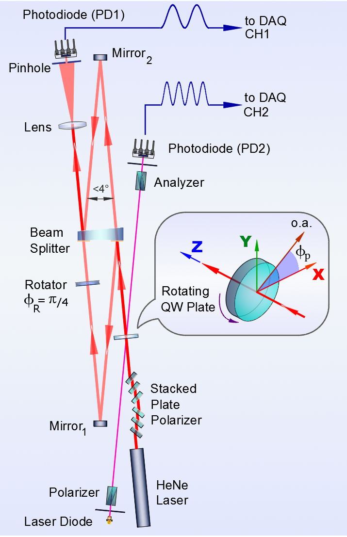
Figure 1: Experimental setup based on a Mach-Zehnder two-arm interferometer with the rotating quarter-wave plate placed before the input beam splitter. The plate in the sample arm (rotator) rotates the plane of polarization of a linear polarized wave by the angle $\Delta\Phi_{R}=\pi/4$.

III.1 Experimental setup

In our setup shown in Fig. 1, a helium-neon laser (the wavelength is $632.8$ nm) with all polarizing elements removed from the resonator was used as a source of unpolarized light. This light was then converted into a partially polarized wave with the prescribed value of the degree of polarization, $P_{0}$, by means of a stacked plate polarizer combined with a series of dichroic polaroids of variable degree of dichroic dye degradation. The polarized part of this wave was linearly polarized along the $x$ axis. Note that each installation of polarizing elements is followed by measurement of the degree of polarization, $P_{0}$, using a combination of a rotating analyzer and a light detector.

Referring to Fig. 1, a beam splitter divides a partially polarized light into two beams, the reference and the testing (sample) beams, which, after reflection at the mirrors $M_{1}$ and $M_{2}$, are recombined at the semireflecting surface of the beam splitter. The interfering beams emerging from the interferometer are projected by the lens onto a screen with a pinhole (the diameter was 150 $\mu$m). After passing the pinhole, light is collected by a photodiode (PD1) (the silicon photodiode OTP101 from Texas Instruments) and the signal is then transmitted to a 12-bit data acquisition system (DAQ).

The interferometer was adjusted to obtain the fringes of equal thickness. Owing to the elongated geometry of the interferometer, all the directions of incidence were close to the normal (deviations from the normal were less than $2^{\circ}$) thus making the polarizing effects of Fresnel reflections negligibly small. The period of the interference pattern was at least $100$ times larger than the pinhole diameter. Hence errors arising from pinhole induced distortions of the intensity profile of interference pattern were below $10^{-3}$. General accuracy of our measurements of the light intensity was affected by errors resulting from mechanical instability and noises of light source, photodiodes and DAQ. This accuracy is estimated to be below $3.0$%.

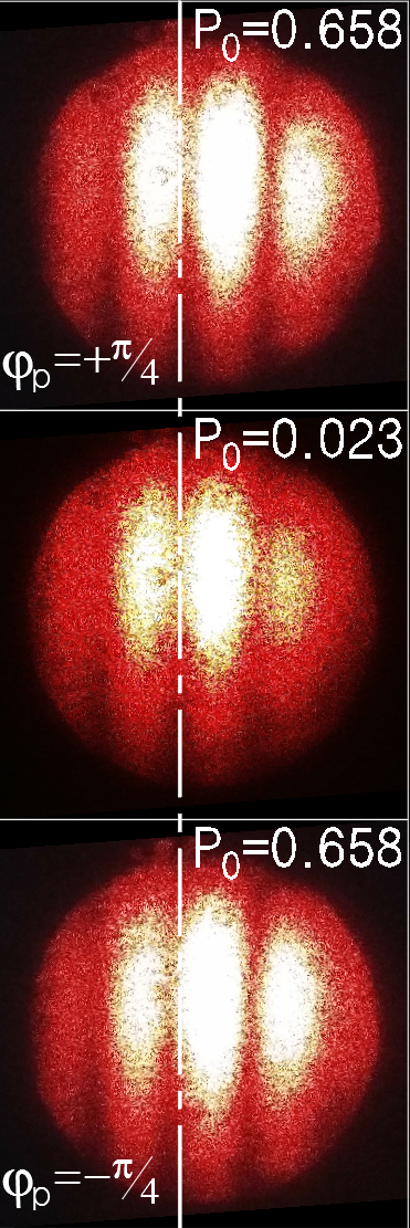
Figure 2: The interference fringes observed in the experimental setup shown in Fig. 1. For nearly-unpolarized light with $P_{0}=0.023$, the pattern is independent of $\phi_{p}$. For partially polarized light with $P_{0}=0.658$, the fringes at $\phi_{p}=\pm\pi/4$ are shifted.

III.2 Interferometer with rotating quarter-wave plate

III.2.1 Experimental procedure

In this setup, the quarter-wave plate (QWP) is placed before the beamsplitter at the input of the interferometer. This plate is rotated about its normal (the frequency was fixed at about $5$ Hz) and orientation of its in-plane optical axis specified by the azimuthal angle, $\phi_{p}$, continuously changes leading to modulation of the polarization state of the partially polarized wave.

In order to get the results that do not rely on the assumption of uniformly rotating QWP, the azimuthal angle $\phi_{p}$ was measured using a crossed polarizers probing scheme [see Fig. 1]. In this scheme, the nearly-normal incident probing wave passes through the QWP placed between the crossed polarizer and the analyzer and the intensity of the transmitted beam is registered by the photodiode (PD2). Since this intensity is known to be proportional to $\sin^{2}(2\phi_{p})$, for our 12-bit DAQ system, the azimuthal angle of the QWP optical axis was measured with excessively high accuracy limited by the noise.

As is illustrated in Fig. 1, by contrast to the reference beam, the testing beam passes through the optically active quartz rotator that rotates the plane of polarization by $45$^∘. The beams are recombined at the beamsplitter to produce the interference pattern.

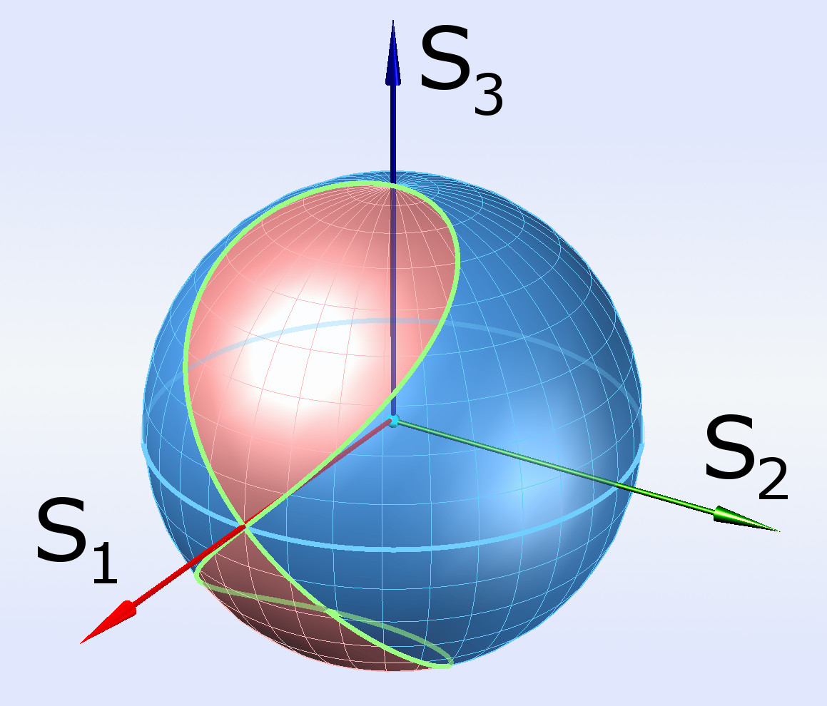
Figure 3: Trajectory on the Poincaré sphere shows the Stokes parameters of light beam passed through the quarter-wave plate (QWP) as a function of the QWP azimuthal angle.

An example of this pattern projected onto the screen is shown in Fig. 2. In general, the contrast and location of the fringes both depend on the QWP azimuthal angle and the degree of polarization, $P_{0}$.

In order to register small shifts of the interference pattern for nearly-unpolarized waves, we need to maximize sensitivity of the measurements. For this purpose, the pinhole is placed at the center of the interval separating adjacent maxima and minima of the pattern. After all preparations, the QW plate was rotated and signals from the photodiodes, PD1 and PD2, were registered and digitized in parallel by the DAQ (CH1 and CH2).

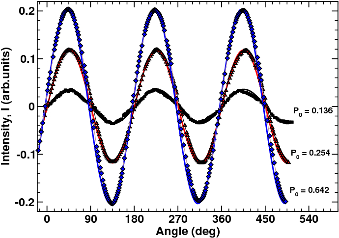
Figure 4: Intensity measured as a function of the QWP azimuthal angle at various values of the degree of polarization. Solid lines represent theoretical curves computed using Eq. (III.2.2) at $\Delta\Phi_{R}=\pi/4$.

III.2.2 Results

An important point to start from is that, for these experiments, the azimuthal angle of the QWP optical axis (the QWP angle) plays the role of the governing parameter: $\phi_{p}=s$. In this subsection, we present theoretical analysis of the experiments along with the experimentally measured data.

By assuming that transmission of light through a birefringent plate is governed by the unitary matrix of the general form:

$$\mathbf{T}_{p}(\phi_{p},\eta_{p})=\mathbf{C}(\pi/4,\phi_{p})\mathrm{e}^{i\eta_{p}\boldsymbol{\sigma}_{3}}{\mathbf{C}}^{\dagger}(\pi/4,\phi_{p})=$$

$$\cos(\eta_{p})\boldsymbol{\sigma}_{0}+i\sin(\eta_{p})\bigl{(}{\hat{\mathbf{m}}_{p}}\cdot{\boldsymbol{\sigma}}\bigr{)},$$ (67)

where $2\eta_{p}=\Delta\Phi_{p}$ is the phase retardation; $\phi_{p}$ is the azimuthal angle of the in-plane principal axes and $\hat{\mathbf{m}}_{p}=(\cos(2\phi_{p}),\sin(2\phi_{p}),0)$, we can describe how the quarter-wave plate (QWP) with $\Delta\Phi_{p}=\pi/2$ modulates the initial polarization state (7) with $\hat{\mathbf{s}}_{0}=\hat{\mathbf{x}}$ and obtain the density matrix of light passed through the plate

$$2\mathbf{T}_{p}\rho_{0}{\mathbf{T}_{p}}^{\dagger}\equiv 2\rho_{p}=\boldsymbol{\sigma}_{0}+P_{0}\bigl{(}{\hat{\mathbf{s}}_{p}}\cdot{\boldsymbol{\sigma}}\bigr{)},$$ (68)

$$\hat{\mathbf{s}}_{p}=\cos(2\phi_{p})\hat{\mathbf{m}}_{p}+\sin(2\phi_{p})\hat{\mathbf{z}}=$$

$$(\sin(2\theta_{p})\cos(2\phi_{p}),\sin(2\theta_{p})\sin(2\phi_{p}),\cos(2\theta_{p})),$$ (69)

where $\theta_{p}=\pi/4-\phi_{p}$ and we have used the algebraic result (100) presented in Appendix A.

The effect of QWP rotation can be visualized as the trajectory of the normalized Stokes vector $\hat{\mathbf{s}}_{p}(s)$ given by Eq. (III.2.2) with $\theta_{p}=\pi/4-s$ and $\phi_{p}=s$ on the Poincaré sphere. As is shown in Fig. 3, this trajectory is figure eight shaped and passes through the poles representing the states of circular polarization.

The density matrix $\rho_{p}$ with the Stokes unit vector given by Eq. (III.2.2) characterizes the reference beam, $\rho_{p}=\rho_{1}$, and can be recast into the following form:

$$2\rho_{p}(s)\equiv 2\rho_{1}(s)=\mathbf{D}_{p}(s)(\boldsymbol{\sigma}_{0}+P_{0}\boldsymbol{\sigma}_{3}){\mathbf{D}}^{\dagger}_{p}(s),$$ (70)

$$\mathbf{D}_{p}(s)\equiv\mathbf{D}_{1}(s)=\mathbf{D}(\phi_{p},\theta_{p},\gamma_{p})=\mathbf{D}(s,\pi/4-s,\mp s),$$ (71)

$$\mathbf{D}(\alpha,\beta,\gamma)=\mathrm{e}^{-i\alpha\boldsymbol{\sigma}_{3}}\mathrm{e}^{-i\beta\boldsymbol{\sigma}_{2}}\mathrm{e}^{-i\gamma\boldsymbol{\sigma}_{3}}.$$ (72)

The components of the eigenpolarization vectors of the reference beam $|{p_{\mu}^{(1)}}\rangle$ are given by the columns of the matrix $\mathbf{D}_{p}(s)=\mathbf{D}_{1}(s)$. In order to make these vectors well-defined at the poles, we have introduced the phase factors for the eigenstates with $\gamma_{p}=-\phi_{p}$ ($\gamma_{p}=\phi_{p}$) for the upper (lower) half of the Poincar’e sphere.

The testing beam is additionally transmitted through the rotator described by the transmission matrix:

$$\mathbf{T}_{R}=\mathrm{e}^{i\Phi_{R}}\mathbf{U}_{R},\>\mathbf{U}_{R}=\mathrm{e}^{i\Delta\Phi_{R}\boldsymbol{\sigma}_{3}}=$$

$$\cos\Delta\Phi_{R}\boldsymbol{\sigma}_{0}+i\sin\Delta\Phi_{R}\boldsymbol{\sigma}_{3}.$$ (73)

The rotator results in rotation of polarization ellipse axes by the angle $\Delta\Phi_{R}$ thus producing the difference between the reference beam with the density matrix $\rho_{1}(s)$ and the testing lightwave which is characterized by the density matrix

$$\rho_{2}(\phi_{p},\theta_{p})=\mathbf{U}_{R}\,\rho_{1}{\mathbf{U}}^{\dagger}_{R}=\rho_{1}(\phi_{p}-\Delta\Phi_{R},\theta_{p})$$ (74)

and the matrix of eigenpolarization vectors

$$\mathbf{D}_{2}=\mathbf{U}_{R}\mathbf{D}_{1}=\mathbf{D}(\phi_{p}-\Delta\Phi_{R},\theta_{p},\gamma_{p}).$$ (75)

The Pancharatnam function (II.1) can now be readily computed as follows

$$\mathrm{e}^{-i\Phi_{R}}F_{P}=\mathop{\rm Tr}\nolimits[\mathbf{U}_{R}\rho_{1}]=$$

$$\cos\Delta\Phi_{R}+iP_{0}\sin\Delta\Phi_{R}\,\cos(2\theta_{p}),$$ (76)

where $\cos(2\theta_{p})=\sin(2s)$.

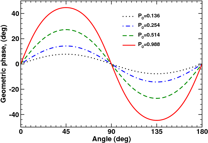
Figure 5: Dependence of the relative geometric phase, $\Phi_{I}=\Phi_{U}^{(12)}$, on the QWP azimuthal angle at different values of the degree of polarization.

We can now insert this formula into Eqs. (15)– (II.1) and calculate the angular dependent part of the output wavefield intensity. This is the intensity which is measured experimentally as described in the previous section and is presented in Fig. 4. Clearly, the theoretical curves shown in Fig. 4 are in excellent agreement with the experimental data.

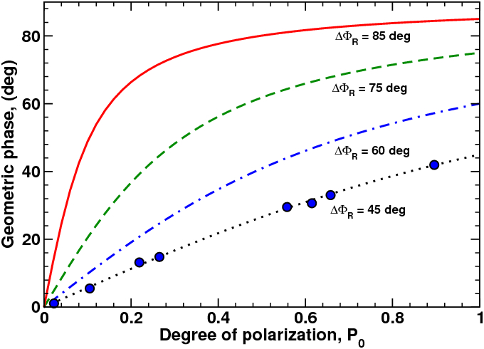
Figure 6: Dependence of the relative geometric phase, $\Phi_{I}=\Phi_{U}^{(12)}$, at $s=\pi/4$ on the degree of polarization at various values of the rotator angle. Experimental points are marked by solid circles.

For unitary evolution, where $\mathbf{A}_{i}={\mathbf{T}}^{\dagger}_{i}\mathbf{T}_{i}=\mathbf{I}$ and $\tilde{\rho}_{i}=\rho_{0}$, the Pancharatnam function (III.2.2) can also be expressed in terms of the eigenstates

$$2F_{P}=\mathrm{e}^{i\Phi_{R}}\sum_{\mu=\pm 1}(1+\mu P_{0})\langle{p_{\mu}^{(1)}(s)}|{p_{\mu}^{(2)}(s)}\rangle,$$ (77)

where

$$\langle{p_{\mu}^{(1)}(s)}|{p_{\mu}^{(2)}(s)}\rangle=\frac{1}{2}\mathop{\rm Tr}\nolimits[(\boldsymbol{\sigma}_{0}+\mu\boldsymbol{\sigma}_{3}){\mathbf{D}}^{\dagger}_{1}\mathbf{U}_{R}\mathbf{D}_{1}]=$$

$$\cos\Delta\Phi_{R}+i\mu\sin\Delta\Phi_{R}\sin(2s),$$ (78)

and the interferometric phase is given by Eq. (61). For the dynamical phases, we have

$$\Phi_{\mu}^{(d)}=\phi_{\mu}^{(2)}-\phi_{\mu}^{(1)},$$ (79)

where

$$\phi_{\mu}^{(i)}=-\frac{i}{2}\mathop{\rm Tr}\nolimits\Bigl{[}(\boldsymbol{\sigma}_{0}+\mu\boldsymbol{\sigma}_{3})\int_{0}^{s}{\mathbf{D}}^{\dagger}_{i}\partial_{\tau}\mathbf{D}_{i}\mathrm{d}\tau\Bigr{]}.$$ (80)

Equation (75) shows that the eigenpolarization vectors of the waves are related through the unitary $\mathbf{U}_{R}$. Since this unitary is independent of the evolution parameter $s$, the operators ${\mathbf{D}}^{\dagger}_{1}\partial_{\tau}\mathbf{D}_{1}$ and ${\mathbf{D}}^{\dagger}_{2}\partial_{\tau}\mathbf{D}_{2}$ [formulas for these operators are given in Eq. (104) of Appendix A] are identical and the difference between the dynamical phases $\phi_{\mu}^{(1)}$ and $\phi_{\mu}^{(2)}$ vanishes. So, the resulting expression for the interferometric phase is

$$\Phi_{I}=\arg[\cos\Delta\Phi_{R}+iP_{0}\sin\Delta\Phi_{R}\,\cos(2s)]=\Phi_{P}-\Phi_{R}.$$ (81)

Now we discuss the relative Uhlmann phase given by Eq. (35). For this purpose, we shall apply the results of Appendix A to our case, where $\mathbf{T}_{1}=\mathbf{T}_{p}$ and $\mathbf{T}_{2}=\mathbf{U}_{R}\mathbf{T}_{1}$. After substituting $\eta=\pi/4$ and $\psi=2s$ into the relation (102), we have

$${\mathbf{T}}^{\dagger}_{1}\partial_{s}\mathbf{T}_{1}={\mathbf{T}}^{\dagger}_{2}\partial_{s}\mathbf{T}_{2}=i\bigl{(}{\mathbf{h}_{p}}\cdot{\boldsymbol{\sigma}}\bigr{)},$$

$$\mathbf{h}_{p}=(-\sin(2s),\cos(2s),1).$$ (82)

At $\hat{\mathbf{s}}_{0}=\hat{\mathbf{x}}$ and $\mathbf{h}=\mathbf{h}_{p}$, formulas (113)– (114) for the Uhlmann connection take the form:

$$\mathbf{H}_{U}^{(1)}=\mathbf{H}_{U}^{(2)}=\bigl{(}{\mathbf{h}_{U}}\cdot{\boldsymbol{\sigma}}\bigr{)},$$ (83)

$$\mathbf{h}_{U}=(1-P_{0}^{2})^{1/2}(\sin(2s)\hat{\mathbf{x}}-\hat{\mathbf{z}})-\cos(2s)\hat{\mathbf{y}}.$$ (84)

From these results it is clear that the Uhlmann holonomies, $\mathbf{V}_{U}^{(1)}$ and $\mathbf{V}_{U}^{(2)}$, are equal and $\mathbf{V}_{U}^{(12)}=\mathbf{I}$. Formulas (35)– (37) then give the relative Uhlmann phase in the simple form:

$$\Phi_{U}^{(12)}(s)=\Phi_{P}(s)-\Phi_{P}(0).$$ (85)

Clearly, it means that the Uhlmann phase (85) is equal to the interferometric phase (81): $\Phi_{U}^{(12)}(s)=\Phi_{I}(s)$.

This is, however, no longer the case for the relative Uhlmann phase, $\tilde{\Phi}_{U}^{(12)}(s)$ given by Eqs. (38)–(40). For this phase, the operator $\mathbf{V}_{12}(0)={\mathbf{T}}^{\dagger}_{2}(0)\mathbf{T}_{1}(0)={\mathbf{T}}^{\dagger}_{1}(0){\mathbf{U}}^{\dagger}_{R}\mathbf{T}_{1}(0)$ that enter Eq. (40) differs from the identity matrix preventing the contributions from the Uhlmann connections of the beams from being canceled out.

In Fig. 5, we present dependence of the relative geometric phase on the QWP azimuthal angle computed from Eq. (81) at various values of the degree of polarization. As it can be seen from Fig. 5, this dependence is perfectly harmonic and the geometric phase is maximal at $\phi_{p}\equiv s=\pi/4$.

Figure 6 shows that the maximum value of the geometric phase is an increasing function of the degree of polarization. Referring to Fig. 6, this dependence becomes more pronounced as the rotator angle $\Delta\Phi_{R}$ approaches $\pi/2$. Though such rotator will suffer from nearly-zero contrast of the fringes.

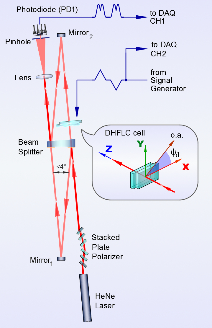
Figure 7: Experimental setup based on a Mach-Zehnder two-arm interferometer with the DHFLC cell (filled with ferroelectric liquid crystal) placed into the testing arm.

III.3 Interferometer with DHFLC cell

In our previous studies Kotova et al. (2015); Kesaev et al. (2017), we have employed the experimental setup based on a Mach-Zehnder interferometer to study electro-optic response of planar aligned deformed-helix ferroelectric liquid crystals (DHFLC) with subwavelength helix pitch.

In such ferroelectric liquid crystals (FLCs), the equilibrium orientational structure forms a helical twisting pattern where FLC molecules align on average along a local unit director $\hat{\mathbf{d}}=\cos\theta\,\hat{\mathbf{h}}+\sin\theta\,\hat{\mathbf{c}},$ where $\theta$ is the smectic tilt angle; $\hat{\mathbf{h}}=\hat{\mathbf{x}}$ is the twisting axis normal to the smectic layers and $\hat{\mathbf{c}}\perp\hat{\mathbf{h}}$ is the $c$-director. The FLC director lies on the smectic cone and rotates in a helical fashion about a uniform twisting axis $\hat{\mathbf{h}}$ forming the FLC helix. The smectic layers are normal to the substrates and the electric field $\mathbf{E}=E\,\hat{\mathbf{z}}$ is applied across the DHFLC cell.

According to Refs. Kiselev et al. (2011); Kiselev and Chigrinov (2014); Kotova et al. (2015); Kiselev (2017), optical properties of such cells can be described by the effective dielectric tensor of a homogenized DHFLC helical structure. The zero-field ($\mathbf{E}=0$) dielectric tensor is uniaxially anisotropic with the optical axis directed along the twisting axis $\hat{\mathbf{h}}=\hat{\mathbf{x}}$. The zero-field effective refractive indices of extraordinary (ordinary) waves, $n_{h}$ ($n_{p}$), generally depend on the smectic tilt angle $\theta$ and the optical dielectric constants characterizing the FLC material (see, e.g., equation (56) in Ref. Kiselev and Chigrinov (2014) giving the expressions for $\epsilon_{h}=n_{h}^{2}$ and $\epsilon_{p}=n_{p}^{2}$).

The electric-field-induced anisotropy is generally biaxial so that the dielectric tensor is characterized by the three generally different principal values: $\epsilon_{\pm}=n_{\pm}^{2}$ and $\epsilon_{z}=n_{z}^{2}$ (see, e.g., equations (60)–(63) in Ref. Kiselev and Chigrinov (2014)). The in-plane principal optical axes, $\hat{\mathbf{d}}_{+}=\cos\psi_{d}\,\hat{\mathbf{x}}+\sin\psi_{d}\,\hat{\mathbf{y}}$ and $\hat{\mathbf{d}}_{-}=\hat{\mathbf{z}}\times\hat{\mathbf{d}}_{+}$, are rotated about the vector of electric field, $\mathbf{E}\parallel\hat{\mathbf{z}}$, by the azimuthal angle $\psi_{\mathrm{d}}$ (see, e.g., equation (64) in Ref. Kiselev and Chigrinov (2014)). This is the so-called orientational Kerr effect which is caused by the electrically induced distortions of the helical structure and is governed by the effective dielectric tensor of a nanostructured chiral smectic liquid crystal defined through averaging over the FLC orientational structure Pozhidaev et al. (2013, 2014); Kiselev et al. (2011); Kiselev and Chigrinov (2014).

III.3.1 Experimental procedure

Our experimental setup with the DHFLC cell placed in the testing arm is depicted in Fig. 7. Orientation of the cell was adjusted so as to have the zero-field optical axis parallel to the $x$ axis (the polarized part of incident lightwave is also linearly polarized along the $x$ axis). The mirrors were fine tuned so as to position the pinhole at the center of a dark fringe in the field-free interference pattern.

Measurements were performed for triangular wave-form of driving voltage with the frequency $f=100$ Hz (alternating triangular pulses with a duty cycle 4/6 ($-\wedge-\vee$)). For this purpose, the signal registered by the photodiode (PD1) was recorded and digitized in parallel with the signal from the generator using the same DAQ (by CH1 and CH2).

Electric field dependence of the light intensity measured at different values of the degree of polarization are presented in Fig. 8. In these experiments we have used the FLC mixture FLC-587F7 (from P.N. Lebedev Physical Institute of Russian Academy of Sciences) as a FLC material for the DHFLC cell (a similar mixture was detailed in Ref. Kotova et al. (2015))

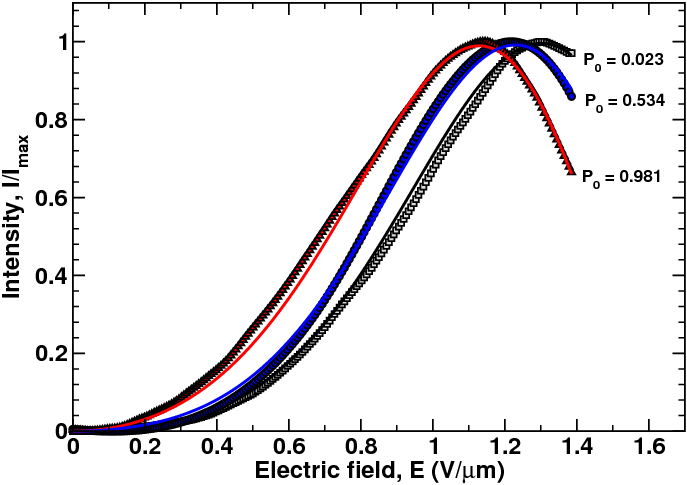
Figure 8: Normalized intensity of output wavefield experimentally measured as a function of the electric field at different values of the degree of polarization, $P_{0}$, for the DHFLC cell of thickness $D\approx 52$ $\mu$m filled with the FLC mixture FLC-587F7. Solid lines represent the theoretical curves. The parameters of the mixture are: $n_{\perp}\approx 1.47$ is the ordinary refractive index, $n_{\parallel}\approx 1.69$ is the extraordinary refractive index, $\theta\approx 33.5$^∘ is the smectic tilt angle, and $r_{2}\approx 1.05$ is the biaxiality ratio.

III.3.2 Results

In the setup shown in Fig. 7, the testing beam propagates through the DHFLC cell which can be regarded as an electrically driven birefringent plate with the unitary transmission matrix $\mathbf{T}$ given by

$$\mathbf{T}_{1}=\mathbf{I},\>\mathbf{T}_{2}=\mathbf{T}(\tau)=\mathbf{C}_{d}\begin{pmatrix}\mathrm{e}^{i\Phi_{+}}&0\\ 0&\mathrm{e}^{i\Phi_{-}}\end{pmatrix}.{\mathbf{C}}^{\dagger}_{d}=$$

$$\mathrm{e}^{i\Phi}\mathbf{T}_{p}(\psi_{d},\Delta\Phi)=\mathrm{e}^{i\Phi}\mathrm{e}^{i\Delta\Phi(\hat{\mathbf{s}}_{d}\cdot\boldsymbol{\sigma})},$$ (86)

where $\mathbf{C}_{d}=\mathbf{C}(\pi/4,\psi_{d})$ and $\Phi_{\pm}=n_{\pm}\tau$; $\Phi=(\Phi_{+}+\Phi_{-})/2$ is the averaged phase shift; $2\Delta\Phi=(n_{+}-n_{-})\tau$ is the difference in optical path of the ordinary and extraordinary waves known as the phase retardation; $\psi_{d}$ is the azimuthal angle of the in-plane optical axis and $\hat{\mathbf{s}}_{d}=(\cos(2\psi_{d}),\sin(2\psi_{d}),0)$. In contrast to the previous section, the governing parameter now is the thickness parameter of the DHFLC cell, $0\leq\tau\leq h\equiv k_{\mathrm{vac}}D$, where $k_{\mathrm{vac}}=\omega/c$ is the free-space wave number and $D$ is the cell thickness.

Thus we have the simple case of unitary evolution with $\mathbf{T}_{1}=\mathbf{T}(0)=\mathbf{I}$ and the Pancharatnam function is given by

$$F_{P}(h)=\mathop{\rm Tr}\nolimits[\rho_{0}\mathbf{T}(h)]=\mathrm{e}^{i\Phi}(\cos(\Delta\Phi)+iP_{0}\sin(\Delta\Phi)$$

$$\times\bigl{(}{\hat{\mathbf{s}}_{d}}\cdot{\hat{\mathbf{s}}_{0}}\bigr{)})=\frac{1}{2}\sum_{\mu=\pm 1}(1+\mu P_{0})\langle{p_{\mu}(0)}|{p_{\mu}(h)}\rangle,$$ (87)

where $|{p_{\mu}(h)}\rangle=\mathbf{T}(h)|{p_{\mu}(0)}\rangle$ is the eigenpolarization vector of the density matrix $\rho_{2}(h)=\mathbf{T}(h)\rho_{0}{\mathbf{T}}^{\dagger}(h)$.

We can now combine the Pancharatnam function (III.3.2) with the known analytical results for $\Phi_{\pm}$ proportional to the effective refractive indices $n_{\pm}$ and the azimuthal angle $\psi_{d}$ describing orientation of the in-plane optical axis (see, e.g., Refs. Kesaev et al. (2017); Kotova et al. (2015); Kiselev and Chigrinov (2014)) to evaluate the intensity of the output field (15) and to fit the experimental data on electric field dependence of the light intensity. Figure 8 presents the experimental results measured by the photodiode at different values of the degree of polarization, $P_{0}$, for the DHFLC cell of thickness $D\approx 52$ $\mu$m filled with the FLC mixture FLC-587F7.

The parameters of the mixture used in the fitting procedure are: $n_{\perp}=\sqrt{\epsilon_{\perp}}\approx 1.47$ is the ordinary refractive index, $n_{\parallel}\approx 1.69$ is the extraordinary refractive index and $\theta\approx 33.5$^∘ is the smectic tilt angle. Then the fitting gives the values of two ratios regarded as the fitting parameters: the ratio of the ferroelectric polarization and the dielectric susceptibility of the Goldstone mode $P_{s}/\chi_{E}\approx 5.43$ V/$\mu$m and the biaxiality ratio $r_{2}=\epsilon_{2}/\epsilon_{\perp}\approx 1.05$, where $\epsilon_{2}$ is the principal value of the dielectric tensor along the FLC polarization vector In Fig. 8, the theoretical curves are shown as solid lines.

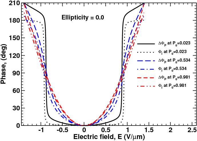
Figure 9: Pancharatnam and interferometric phases, $\Delta\Phi_{P}=\Phi_{P}(E)-\Phi_{P}(0)$ and $\Phi_{I}$, as a function of the electric field at different values of the degree of polarization, $P_{0}$.

III.3.3 Geometric phases

Now we proceed with the geometric phases. Our task is to compute the phases as a function of the applied electric field by using the experimental data combined with the results of fitting obtained in Sec. III.3.2.

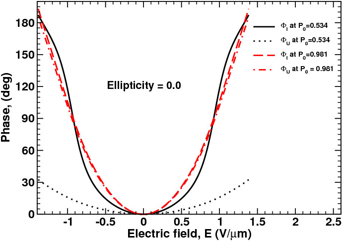
Figure 10: Electric field dependence of Uhlmann and interferometric phases, $\Phi_{U}$ and $\Phi_{I}$, at different values of the degree of polarization, $P_{0}$.

We begin with calculation of the interferometric phase. For this purpose, we compute the inner products

$$\langle{p_{\mu}(0)}|{p_{\mu}(h)}\rangle=\frac{1}{2}\mathop{\rm Tr}\nolimits[(\boldsymbol{\sigma}_{0}+\mu\boldsymbol{\sigma}_{3}){\mathbf{C}}^{\dagger}_{0}\mathbf{T}(h)\mathbf{C}_{0}]=$$

$$\mathrm{e}^{i\Phi}(\cos\Delta\Phi+i\mu\,\sin\Delta\Phi\bigl{(}{\hat{\mathbf{s}}_{d}}\cdot{\hat{\mathbf{s}}_{0}}\bigr{)}),$$ (88)

and the dynamical phases

$$\Phi_{\mu}^{(d)}=-\frac{i}{2}\int_{0}^{h}\mathop{\rm Tr}\nolimits[(\boldsymbol{\sigma}_{0}+\mu\boldsymbol{\sigma}_{3}){\mathbf{C}}^{\dagger}_{0}{\mathbf{T}}^{\dagger}(\tau)\dot{\mathbf{T}}(\tau)\mathbf{C}_{0}]\mathrm{d}\tau$$

$$=-i\int_{0}^{h}\langle{p_{\mu}(\tau)}|\partial_{\tau}|{p_{\mu}(\tau)}\rangle\mathrm{d}\tau=\Phi+\mu\,\Delta\Phi\bigl{(}{\hat{\mathbf{s}}_{d}}\cdot{\hat{\mathbf{s}}_{0}}\bigr{)},$$ (89)

where we have used the identity: $-i{\mathbf{T}}^{\dagger}\dot{\mathbf{T}}=\mathbf{H}=\dot{\Phi}\,\boldsymbol{\sigma}_{0}+\Delta\dot{\Phi}\,\bigl{(}{\hat{\mathbf{s}}_{d}}\cdot{\boldsymbol{\sigma}}\bigr{)}$ for the transmission matrix (III.3.2), that enter the interferometric function

$$2F_{I}=\sum_{\mu=\pm 1}(1+\mu P_{0})\langle{p_{\mu}(0)}|{p_{\mu}(h)}\rangle\mathrm{e}^{-i\Phi_{\mu}^{(d)}}.$$ (90)

After substituting formulas (III.3.3) and (III.3.3) into Eq. (90), we obtain the interferometric phase in the following form:

$$\Phi_{I}=\arg(\mathop{\rm Re}\nolimits\tilde{F}_{I}+iP_{0}\mathop{\rm Im}\nolimits\tilde{F}_{I}),$$ (91)

$$\tilde{F}_{I}=[\cos(\Delta\Phi)+i\sin(\Delta\Phi)\bigl{(}{\hat{\mathbf{s}}_{d}}\cdot{\hat{\mathbf{s}}_{0}}\bigr{)}]\mathrm{e}^{-i\Delta\Phi(\hat{\mathbf{s}}_{d}\cdot\hat{\mathbf{s}}_{0})}.$$ (92)

The phases (III.3.3) can also be used to evaluate the interferometric holonomy (57) at $\mathbf{V}_{I}^{(2)}=\mathbf{I}$ and $|{r_{\mu}^{(i)}}\rangle=|{p_{\mu}(0)}\rangle$. The result reads

$$\mathbf{V}_{I}=\mathrm{e}^{-i\Phi}\mathrm{e}^{-i\Delta\Phi(\hat{\mathbf{s}}_{d}\cdot\hat{\mathbf{s}}_{0})(\hat{\mathbf{s}}_{0}\cdot\boldsymbol{\sigma})}.$$ (93)

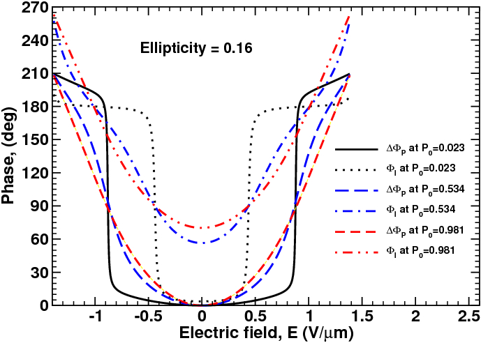
Figure 11: Electric field dependence of the Pancharatnam and interferometric phases, $\Phi_{P}$ and $\Phi_{I}$, for elliptically polarized waves with $\epsilon_{\mathrm{ell}}=\tan(\pi/4-\theta_{0})\approx 0.16$ ($\theta_{0}=36^{\circ}$) at different values of the degree of polarization, $P_{0}$.

Now we turn to the Uhlmann phase. By applying the results of Appendix A to our case with $\mathbf{H}=\dot{\Phi}\,\boldsymbol{\sigma}_{0}+\Delta\dot{\Phi}\,\bigl{(}{\hat{\mathbf{s}}_{d}}\cdot{\boldsymbol{\sigma}}\bigr{)}$ we deduce the Uhlmann connection

$$\mathbf{H}_{U}=-\dot{\Phi}\boldsymbol{\sigma}_{0}-\Delta\dot{\Phi}\bigl{(}{\mathbf{q}_{U}}\cdot{\boldsymbol{\sigma}}\bigr{)},$$ (94)

$$\mathbf{q}_{U}=(1-P_{0}^{2})^{1/2}[\hat{\mathbf{s}}_{d}-\bigl{(}{\hat{\mathbf{s}}_{d}}\cdot{\hat{\mathbf{s}}_{0}}\bigr{)}\hat{\mathbf{s}}_{0}]+\bigl{(}{\hat{\mathbf{s}}_{d}}\cdot{\hat{\mathbf{s}}_{0}}\bigr{)}\hat{\mathbf{s}}_{0},$$ (95)

where $|\mathbf{q}_{U}|^{2}=1-P_{0}^{2}(1-\bigl{(}{\hat{\mathbf{s}}_{d}}\cdot{\hat{\mathbf{s}}_{0}}\bigr{)}^{2})$, and the corresponding Uhlmann holonomy

$$\mathbf{V}_{U}=\mathrm{e}^{-i\Phi}\mathrm{e}^{-i\Delta\Phi(\mathbf{q}_{U}\cdot\boldsymbol{\sigma})},$$ (96)

so that the Uhlmann phase is given by

$$\Phi_{U}=\arg F_{U}^{(12)}\equiv\arg F_{U}$$

$$=\arg\mathop{\rm Tr}\nolimits[\sqrt{\rho_{0}}\,\mathrm{e}^{i\Delta\Phi(\hat{\mathbf{s}}_{d}\cdot\boldsymbol{\sigma})}\sqrt{\rho_{0}}\,\mathrm{e}^{-i\Delta\Phi(\mathbf{q}_{U}\cdot\boldsymbol{\sigma})}].$$ (97)

As is evident from a comparison between formulas (93) and (96), the holonomies become identical in the limiting case of pure states with $P_{0}=1$. It is also clear that, by contrast to the interferometric holonomy (93), the Uhlmann holonomy (96) depends on the degree of polarization and does not commute with the density matrix $\rho_{0}$.

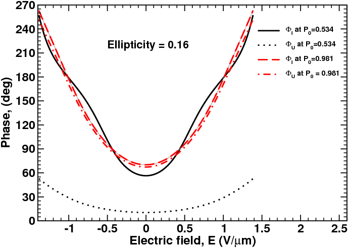
Figure 12: Electric field dependence of the Uhlmann and interferometric phases, $\Phi_{U}$ and $\Phi_{I}$, for elliptically polarized waves with $\epsilon_{\mathrm{ell}}=\tan(\pi/4-\theta_{0})\approx 0.16$ ($\theta_{0}=36^{\circ}$) at different values of the degree of polarization, $P_{0}$.

Figure 9 shows how the Pancharatnam and interferometric phases depend on the electric field applied across the DHFLC cell. The curves presented in Fig. 9 are computed from Eq. (III.3.2) and Eq. (91) using the parameters of the DHFLC cell that was derived by fitting the experimental results [see Fig. 8]. As can be seen from Fig. 9, the electrically induced parts of the phases are close to each other and the difference between the curves decreases with the degree of polarization.

The results for the Uhlmann and the interferometric phases are shown in Fig. 10. By contrast to the interferometric phase, the Uhlmann phase is negligibly small when the incident wave is nearly-unpolarized with $P_{0}=0.023$. As it has already been mentioned, the phases are coincident in the limiting case of fully polarized waves with $P_{0}=1$ and, as is shown in Fig. 10, there is little difference between the curves at $P_{0}=0.981$.

Ellipticity of the polarized part of the input wave, $\epsilon_{\mathrm{ell}}=\tan(\pi/4-\theta_{0})$, is determined by the polar angle, $\theta_{0}$, of the Stokes vector (6). Figures 11 and 12 demonstrate what happen to the phases at non-vanishing ellipticity. Referring to Fig. 11, in contrast to the case of linear polarization, the curves for the Pancharatnam and the interferometric phases are no longer close to each other. From similar curves for the Uhlmann phase shown in Fig. 12 it might be concluded that $\Phi_{I}$ is the phase most sensitive to variations in the ellipticity as compared to the Pancharatnam and Uhlmann phases.

In closing this subsection, note that, in Appendix B, we discuss how to take into account the effects of dissipation in birefringent plates and derive the analytical results for the Uhlmann and interferometric phases.

IV Discussion and conclusions

In this paper, we have studied the Uhlmann and interferometric phases of mixed polarization states within the framework of the interferometry of partially polarized waves. This interferometry based approach assumes that the partially polarized beams independently evolve and, depending on their dynamics (evolution), acquire both dynamical and geometric phases. These beams brought together emerge from the interferometer producing the interference pattern where loci of fringes are determined by the Pancharatnam phase expressed in terms of the Pancharatnam function (II.1).

Recasting this function into the form of inner product of the amplitudes (purifications) gives the relation (21) linking the Uhlmann approach and the interference pattern. The relative Uhlmann phase (33) defined in terms of the parallel-transported amplitudes (34) then appears as a natural consequence of this relation.

Alternatively, the Pancharatnam function can be written as a superposition of inner products of the eigenstates (II.3). We have found that the structure of this superposition is complicated in the presence of dissipation (nonunitary evolution). A simpler form of this superposition (see, e.g., Eq. (III.3.2)) was used as a starting point of the method giving the interferometric phase for both types of evolution Sjöqvist et al. (2000); Tong et al. (2004). Following this method, we have eliminated the dynamical phases of the eigenstates and derived the interferometric phase (55). Similar form of our key results for the relative Uhlmann phase [see Eqs. (35)– (37)] and the interferometric phase [see Eqs. (55)–(57)] clearly indicate that the Uhlmann and interferometric holonomies determined by different parallel transport conditions [see Eq. (24) and Eq. (45)] are responsible for differences between the phases.

In our experimental investigation into the effects of the degree of polarization in modulation of partially polarized light we have employed the well-known technique based a Mach-Zehnder two-arm interferometer. Two different dynamical regimes of light modulation are studied: (a) modulation of the input wave by the rotating quarter-wave plate (see Fig. 1); and (b) modulation of the testing beam by the deformed-helix ferroelectric liquid crystal cell that can be viewed as a birefringent plate with electrically controlled anisotropy (see Fig. 8).

In the setup using the rotating QWP, modulation dynamics is governed by the azimuthal angle of the QWP transmission axis $\phi_{p}$ which is regarded as the governing parameter and the normalized Stokes vector describing the polarized part of the input wave (see Eq. (III.2.2)) moves along the figure eight shaped trajectory on the Poincaré sphere as the QWP angle varies (see Fig. 3). The testing beam additionally passes through the rotator made of quartz that rotates the plane of polarization by the angle $\Delta\Phi_{R}=\pi/4$. The interference pattern is found to be determined by the Pancharatnam function (77) which is used to perform computations giving the output in excellent agreement with the experimental data. Our analysis led to the conclusion that the interferometric and the relative Uhlmann phases are equal and the geometric phase is the phase extracted from the results of our measurements using the Pancharatnam function (77). Figures 5 and 6 show how the geometric phase depends on the QWP angle and the degree of polarization, respectively.

In our experiments where the partially polarized testing light is modulated by the DHFLC cell light modulation takes place due to the orientational Kerr effect in ferroelectric liquid crystals. The DHFLC cell regarded as an optical device represents a birefringent plate with electrically controlled anisotropy and the physics of the orientational Kerr effect defines how the phase shifts ($\Phi_{\pm}$ in Eq. (III.3.2)) and orientation of the optical axes (the azimuthal angle $\psi_{d}$ in Eq. (III.3.2)) depend on the applied electric field.

The results of a comprehensive theoretical treatment of this effect performed in Ref. Kiselev and Chigrinov (2014) are reviewed in Ref. Kiselev (2017). Similarly to Ref. Kotova et al. (2015), where electro-optic response of DHFLC was studied for unpolarized light, we have used these results to fit the experimental data (see Fig. 8) and to evaluate electric field dependencies of the geometric phases using the parameters obtained from the fitting procedure (see Figs. 9–12).

Referring to Fig. 9, the interferometric phase appears to be close to the Pancharatnam phase when the polarized part of the input wave is linearly polarized. From a comparison between the Uhlmann and interferometric phases plotted in Fig. 10, it can be inferred that a considerable difference between the phases at relatively low degrees of polarization vanishes in the limit of pure state (fully polarized wave) with $P_{0}\to 1$. Figures 11 and 12 demonstrate sensitivity of the interferometric phase to the ellipticity of the incident light as compared to the Pancharatnam and the Uhlmann phases.

Our concluding remark concerns the interferometric phase in the regime of nonunitary dynamics. From formula (60), the dynamical phases that determine the interferometric holonomies can, similar to the case of unitary evolution, be expressed solely in terms of the eigenpolarization states of the density matrix. Analytical results presented in Appendix B describe how the phases of the electrically controlled birefringent plate are affected by the dissipation (nonunitarity) effects such as absorption or Fresnel reflections. A more comprehensive analysis and experimental studies of such effects are now in progress.

Appendix A Uhlmann connection

In this Appendix we present details on computing Uhlmann connection $\mathbf{H}_{U}$ for the unitary operators of the form:

$$\mathbf{T}=\mathrm{e}^{i\eta(\hat{\mathbf{m}}\cdot\boldsymbol{\sigma})}=\cos\eta\,\boldsymbol{\sigma}_{0}+i\sin\eta\,\bigl{(}{\hat{\mathbf{m}}}\cdot{\boldsymbol{\sigma}}\bigr{)},$$ (98)

where $\hat{\mathbf{m}}=\hat{\mathbf{m}}(\psi)$ and the angles $\eta$ and $\psi$ are generally functions of the governing parameter. Such operators represent birefringent plates and we can use the algebraic identity

$$\bigl{(}{\hat{\mathbf{s}}_{0}}\cdot{\boldsymbol{\sigma}}\bigr{)}\bigl{(}{\hat{\mathbf{m}}}\cdot{\boldsymbol{\sigma}}\bigr{)}=\bigl{(}{\hat{\mathbf{s}}_{0}}\cdot{\hat{\mathbf{m}}}\bigr{)}\boldsymbol{\sigma}_{0}+i\bigl{(}{\hat{\mathbf{s}}_{0}\times\hat{\mathbf{m}}}\cdot{\boldsymbol{\sigma}}\bigr{)}$$ (99)

to derive the density matrix of light passed through such a plate in the following form:

$$2\mathbf{T}\rho_{0}{\mathbf{T}}^{\dagger}\equiv 2\rho_{\eta}=\boldsymbol{\sigma}_{0}+P_{0}\bigl{(}{\hat{\mathbf{s}}_{\eta}}\cdot{\boldsymbol{\sigma}}\bigr{)},$$ (100)

$$\hat{\mathbf{s}}_{\eta}=\cos(2\eta)\hat{\mathbf{s}}_{0}+(1-\cos(2\eta))\bigl{(}{\hat{\mathbf{s}}_{0}}\cdot{\hat{\mathbf{m}}}\bigr{)}\hat{\mathbf{m}}+$$

$$\sin(2\eta)\hat{\mathbf{s}}_{0}\times\hat{\mathbf{m}}.$$ (101)

We can also use the identity (99) to calculate the operator $\mathbf{H}$

$${\mathbf{T}}^{\dagger}\dot{\mathbf{T}}=i\mathbf{H},\quad\mathbf{H}=\bigl{(}{\mathbf{q}}\cdot{\boldsymbol{\sigma}}\bigr{)},\quad\mathbf{q}=\dot{\eta}\,\hat{\mathbf{m}}+\dot{\psi}\sin\eta\,\mathbf{n},$$ (102)

$$\mathbf{n}=\cos\eta\,\hat{\mathbf{m}}^{\prime}_{\psi}+\sin\eta\,\hat{\mathbf{m}}\times\hat{\mathbf{m}}^{\prime}_{\psi},$$ (103)

where $\hat{\mathbf{m}}^{\prime}_{\psi}=\partial_{\psi}\hat{\mathbf{m}}$ and dot over the letter denotes the derivative with respect to the governing parameter, that enter equation (27) for the Uhlmann connection.

The relation (102) can be generalized to the case of the Wigner operators $\mathbf{D}(\alpha,\beta,\gamma)$ [see Eq. (72)] with the angles being a function of the governing parameter. In this case, we have

$${\mathbf{D}}^{\dagger}\dot{\mathbf{D}}=-i\mathbf{H}_{D},\quad\mathbf{H}_{D}=\bigl{(}{\mathbf{d}}\cdot{\boldsymbol{\sigma}}\bigr{)},$$ (104)

$$d_{1}=-\dot{\alpha}\sin(2\beta)\cos(2\gamma)+\dot{\beta}\sin(2\gamma),$$

$$d_{2}=\dot{\beta}\cos(2\gamma),\>d_{3}=\dot{\alpha}\cos(2\beta)+\dot{\gamma}.$$ (105)

These results can be obtained using the algebraic identities for the $1/2$-spin Wigner matrices Varshalovich et al. (1988) written in the following form:

$$\mathbf{D}\boldsymbol{\sigma}_{i}{\mathbf{D}}^{\dagger}=\bigl{(}{\hat{\mathbf{m}}_{i}}\cdot{\boldsymbol{\sigma}}\bigr{)},$$ (106)

$${\mathbf{D}}^{\dagger}\boldsymbol{\sigma}\mathbf{D}=\hat{\mathbf{m}}_{1}\boldsymbol{\sigma}_{1}+\hat{\mathbf{m}}_{2}\boldsymbol{\sigma}_{2}+\hat{\mathbf{m}}_{3}\boldsymbol{\sigma}_{3},$$ (107)

where $\hat{\mathbf{m}}_{1}=\cos(2\gamma)\hat{\mathbf{s}}_{1}+\sin(2\gamma)\hat{\mathbf{s}}_{2}$, $\hat{\mathbf{m}}_{2}=-\sin(2\gamma)\hat{\mathbf{s}}_{1}+\cos(2\gamma)\hat{\mathbf{s}}_{2}$, and $\hat{\mathbf{m}}_{3}=\hat{\mathbf{s}}_{3}$; the columns of the rotation matrix

$$\mathbf{S}=\begin{pmatrix}\cos(2\beta)\cos(2\alpha)&-\sin(2\alpha)&\sin(2\beta)\cos(2\alpha)\\ \cos(2\beta)\sin(2\alpha)&\cos(2\alpha)&\sin(2\beta)\sin(2\alpha)\\ -\sin(2\beta)&0&\cos(2\beta)\end{pmatrix}$$ (108)

give the components of $\hat{\mathbf{s}}_{i}$: $\hat{\mathbf{s}}_{i}=\sum_{k}\mathbf{S}_{ki}\hat{\mathbf{e}}_{k}$.

For unitary evolution with $\mathbf{A}=\mathbf{I}$ and $\tilde{\rho}=\rho_{0}$, Eq. (27) assumes the simplified form:

$$2\sqrt{\rho_{0}}\mathbf{H}\sqrt{\rho_{0}}=-[\mathbf{H}_{U},\rho_{0}]_{+}.$$ (109)

In the basis of eigenstates of the density matrix $\rho_{0}$ we have

$${\mathbf{C}}^{\dagger}_{0}\mathbf{H}\mathbf{C}_{0}=\bigl{(}{\mathbf{q}}\cdot{\hat{\mathbf{s}}_{1}}\bigr{)}\boldsymbol{\sigma}_{1}+\bigl{(}{\mathbf{q}}\cdot{\hat{\mathbf{s}}_{2}}\bigr{)}\boldsymbol{\sigma}_{2}+\bigl{(}{\mathbf{q}}\cdot{\hat{\mathbf{s}}_{0}}\bigr{)}\boldsymbol{\sigma}_{3}$$ (110)

$${\mathbf{C}}^{\dagger}_{0}\mathbf{H}_{U}\mathbf{C}_{0}=\tilde{q}_{1}\boldsymbol{\sigma}_{1}+\tilde{q}_{2}\boldsymbol{\sigma}_{2}+\tilde{q}_{3}\boldsymbol{\sigma}_{3},$$ (111)

$$(1-P_{0}^{2})^{1/2}(\bigl{(}{\mathbf{q}}\cdot{\hat{\mathbf{s}}_{1}}\bigr{)}\boldsymbol{\sigma}_{1}+\bigl{(}{\mathbf{q}}\cdot{\hat{\mathbf{s}}_{2}}\bigr{)}\boldsymbol{\sigma}_{2})+2\bigl{(}{\mathbf{q}}\cdot{\hat{\mathbf{s}}_{0}}\bigr{)}\boldsymbol{\sigma}_{3}\rho_{0}=$$

$$-(\tilde{q}_{1}\boldsymbol{\sigma}_{1}+\tilde{q}_{2}\boldsymbol{\sigma}_{2})-2\tilde{q}_{3}\boldsymbol{\sigma}_{3}\rho_{0},$$ (112)

where $2\boldsymbol{\sigma}_{3}\rho_{0}=P_{0}\boldsymbol{\sigma}_{0}+\boldsymbol{\sigma}_{3}$ and equation (A) is derived from Eq. (109). It is not difficult to find the components of the operator (111): $\tilde{q}_{1,2}=-(1-P_{0}^{2})^{1/2}\bigl{(}{\mathbf{h}}\cdot{\hat{\mathbf{s}}_{1,2}}\bigr{)}$ and $\tilde{q}_{3}=-\bigl{(}{\mathbf{h}}\cdot{\hat{\mathbf{s}}_{0}}\bigr{)}$. Turning back to the circular basis can be performed by replacing $\boldsymbol{\sigma}_{i}$ with $\bigl{(}{\hat{\mathbf{s}}_{i}}\cdot{\boldsymbol{\sigma}}\bigr{)}$. The resulting expression for the Uhlmann connection reads

$$\mathbf{H}_{U}=\bigl{(}{\mathbf{q}_{U}}\cdot{\boldsymbol{\sigma}}\bigr{)}=\tilde{q}_{1}\bigl{(}{\hat{\mathbf{s}}_{1}}\cdot{\boldsymbol{\sigma}}\bigr{)}+\tilde{q}_{2}\bigl{(}{\hat{\mathbf{s}}_{2}}\cdot{\boldsymbol{\sigma}}\bigr{)}+\tilde{q}_{2}\bigl{(}{\hat{\mathbf{s}}_{1}}\cdot{\boldsymbol{\sigma}}\bigr{)},$$ (113)

$$\mathbf{q}_{U}=-(1-P_{0}^{2})^{1/2}\mathbf{q}-[1-(1-P_{0}^{2})^{1/2}]\bigl{(}{\mathbf{q}}\cdot{\hat{\mathbf{s}}_{0}}\bigr{)}\hat{\mathbf{s}}_{0}.$$ (114)

Note that, for operators of the form: $\mathbf{B}=b_{0}\boldsymbol{\sigma}_{0}+\bigl{(}{\mathbf{b}}\cdot{\boldsymbol{\sigma}}\bigr{)}$, considerations along similar lines lead to the following relation:

$$2\sqrt{\rho_{0}}\mathbf{B}\sqrt{\rho_{0}}=(1-P_{0}^{2})^{1/2}\mathbf{B}+$$

$$\bigl{\{}[1-({1-P_{0}^{2}})^{1/2}]\bigl{(}{\mathbf{b}}\cdot{\hat{\mathbf{s}}_{0}}\bigr{)}+P_{0}b_{0}\bigr{\}}\bigl{(}{\hat{\mathbf{s}}_{0}}\cdot{\boldsymbol{\sigma}}\bigr{)}+$$

$$\bigl{\{}P_{0}\bigl{(}{\mathbf{b}}\cdot{\hat{\mathbf{s}}_{0}}\bigr{)}+[1-({1-P_{0}^{2}})^{1/2}]b_{0}\bigr{\}}\boldsymbol{\sigma}_{0}.$$ (115)

Appendix B Phases for birefringent plates and effects of dissipation

In this Appendix we relax the assumption of lossless transmission and extend our analysis presented in Sec. III.3 to a more general case of a birefringent plate characterized by the nonunitary transmission matrix

$$\mathbf{T}(\tau)=\mathbf{C}_{d}\mathbf{T}_{d}\mathbf{U}_{d}{\mathbf{C}}^{\dagger}_{d},$$

$$\mathbf{T}_{d}=\begin{pmatrix}t_{+}&0\\ 0&t_{-}\end{pmatrix},\>\mathbf{U}_{d}=\begin{pmatrix}\mathrm{e}^{i\Phi_{+}}&0\\ 0&\mathrm{e}^{i\Phi_{-}}\end{pmatrix},$$ (116)

where $\mathbf{C}_{d}=\mathbf{C}(\pi/4,\psi_{d})$ and $0\leq t_{\pm}\leq 1$ are the transmittance coefficients that take into account the effects of losses such as Fresnel reflections or absorption. In the limiting case of unitary (lossless) evolution analyzed in Sec. III.3 these coefficients are both equal to unity: $t_{\pm}=1$ and we obtain the transmission matrix of the DHFLC cell given by Eq. (III.3.2).

B.1 Interferometric phase

We begin with the interferometric phase. Computing the interferometric phase involves three steps: (a) solving the spectral problem for the density matrix $\rho(\tau)=\mathbf{T}(\tau)\rho_{0}{\mathbf{T}}^{\dagger}(\tau)$ to find the eigenpolarization vectors $|{p_{\mu}(\tau)}\rangle$ and eigenvalues $p_{\mu}(\tau)$; (b) evaluating the dynamical phase (60); and (c) substituting the unitary operator (52) into the expression for the interferometric function (II.3).

Our starting point is the expression for the density matrix given by

$$\frac{2}{r_{+}}{\mathbf{V}}^{\dagger}_{d}\,\rho(\tau)\,\mathbf{V}_{d}=q_{0}^{(\rho)}\boldsymbol{\sigma}_{0}+\bigl{(}{\mathbf{q}_{\rho}}\cdot{\boldsymbol{\sigma}}\bigr{)},$$ (117)

$$q_{0}^{(\rho)}=1+rP_{0}\bigl{(}{\hat{\mathbf{s}}_{0}}\cdot{\hat{\mathbf{s}}_{d}}\bigr{)},\>q_{3}^{(\rho)}=r+P_{0}\bigl{(}{\hat{\mathbf{s}}_{0}}\cdot{\hat{\mathbf{s}}_{d}}\bigr{)},$$

$$q_{1,2}^{(\rho)}=P_{0}\sqrt{1-r^{2}}\bigl{(}{\hat{\mathbf{s}}_{0}}\cdot{\hat{\mathbf{s}}_{1,2}^{(d)}}\bigr{)},$$ (118)

$$r=\frac{r_{-}}{r_{+}}=\frac{t_{+}^{2}-t_{-}^{2}}{t_{+}^{2}+t_{-}^{2}},$$ (119)

where $\mathbf{V}_{d}=\mathbf{C}_{d}\mathbf{U}_{d}$ and $r_{\pm}=(t_{+}^{2}\pm t_{-}^{2})/2$; $\hat{\mathbf{s}}_{1}^{(d)}=(0,0,-1)$ and $\hat{\mathbf{s}}_{2}^{(d)}=(-\sin(2\psi_{d}),\cos(2\psi_{d}),0)$. We can now use the identities (10) for the $1/2$-spin Wigner rotation martrices to diagonalize the matrix (117) as follows

$${\mathbf{C}}^{\dagger}_{\rho}\bigl{(}{\mathbf{q}_{\rho}}\cdot{\boldsymbol{\sigma}}\bigr{)}\mathbf{C}_{\rho}=|\mathbf{q}_{\rho}|\boldsymbol{\sigma}_{3},\>\mathbf{C}_{\rho}\equiv\mathbf{C}(\phi_{\rho},\theta_{\rho}),$$ (120)

where

$$\cos(2\theta_{\rho})=\frac{r+P_{0}\bigl{(}{\hat{\mathbf{s}}_{0}}\cdot{\hat{\mathbf{s}}_{d}}\bigr{)}}{|\mathbf{q}_{\rho}|},$$ (121)

$$|\mathbf{q}_{\rho}|^{2}=P_{0}^{2}(1-r^{2})\bigl{[}1-\bigl{(}{\hat{\mathbf{s}}_{0}}\cdot{\hat{\mathbf{s}}_{d}}\bigr{)}^{2}\bigr{]}$$

$$+\bigl{[}r+P_{0}\bigl{(}{\hat{\mathbf{s}}_{0}}\cdot{\hat{\mathbf{s}}_{d}}\bigr{)}\bigr{]}^{2}.$$ (122)

At this stage, we have the matrix of eigenpolarization vectors

$$\mathbf{V}_{\rho}=\mathbf{V}_{d}\mathbf{C}_{\rho}$$ (123)

and the eigenvalues of the density matrix

$$p_{\mu}(\tau)=\frac{r_{+}}{2}\bigl{(}q_{0}^{(\rho)}+\mu|\mathbf{q}_{\rho}|\bigr{)}\equiv\frac{\mathop{\rm Tr}\nolimits\rho}{2}(1+\mu\,P),$$ (124)

where $P=|\mathbf{q}_{\rho}|/q_{0}^{(\rho)}$ is the degree of polarization. Note that, in Eqs. (B.1)– (123), the transmittance anisotropy parameter $r$ [see Eq. (119)] is the only parameter describing nonunitarity effects. These effects also result in reduction of the transmitted light intensity, so that the trace of the density matrix $\mathop{\rm Tr}\nolimits\rho(\tau)=r_{+}q_{0}^{(\rho)}$ is generally differ from unity.

For the eigenpolarization vectors (123) and the transmission matrix (B), it is not difficult to obtain the dynamical phases

$$\Phi_{\mu}^{(d)}=\mathop{\rm Im}\nolimits\int_{0}^{h}\langle{p_{\mu}}|\dot{\mathbf{T}}\mathbf{T}^{-1}|{p_{\mu}}\rangle\mathrm{d}\tau=\Phi+\mu{\Phi}_{d},$$

$${\Phi}_{d}=\int_{0}^{h}\cos(2\theta_{\rho})\Delta\dot{\Phi}(\tau)\mathrm{d}\tau,$$ (125)

giving the interferometric function

$$F_{I}=\mathop{\rm Tr}\nolimits[\rho_{0}\tilde{\mathbf{V}}_{I}(h)\mathbf{T}(h)]$$

$$=\mathop{\rm Tr}\nolimits\left\{\tilde{\mathbf{V}}_{I}(h)\rho(h)[{\mathbf{T}}^{\dagger}(h)]^{-1}\right\}$$

$$=\sum_{\mu=\pm 1}\mathrm{e}^{-i\Phi_{\mu}^{(d)}}p_{\mu}\langle{p_{\mu}}|[{\mathbf{T}}^{\dagger}]^{-1}|{p_{\mu}}\rangle$$

$$=\frac{\mathop{\rm Tr}\nolimits\rho}{2}\sum_{\mu=\pm 1}\mathrm{e}^{-i\mu{\Phi}_{d}}(1+\mu\,P)[t_{0}+\mu\,t_{3}\cos(2\theta_{\rho})],$$ (126)

where

$$\mathbf{T}_{d}^{-1}\mathbf{U}_{d}=\mathrm{e}^{i\Phi}(t_{0}\boldsymbol{\sigma}_{0}+t_{3}\boldsymbol{\sigma}_{3}),$$ (127)

that defines the interferometric phase: $\Phi_{I}=\arg F_{I}$. It can be checked that, in the unitary limit with $r=0$, formula (B.1) reproduces the result given by Eq. (90) of Sec. III.3.

B.2 Uhlmann phase

Now we turn to the Uhlmann phase and start with computing the Uhlmann connection. This connection can be found by solving Eq. (27). After evaluating the operators that enter both sides of this equation, we find that, similar to Eq. (109), it can be written in the form:

$$2\mathbf{H}=-[\mathbf{H}_{U},\tilde{\rho}]_{+},$$ (128)

where

$$\mathbf{H}=\sqrt{\rho_{0}}\mathbf{H}_{0}\sqrt{\rho_{0}},\>\mathbf{H}_{0}=\mathbf{C}_{d}\begin{pmatrix}t_{+}^{2}\dot{\psi}_{+}&0\\ 0&t_{-}^{2}\dot{\psi}_{-}\end{pmatrix}{\mathbf{C}}^{\dagger}_{d},$$ (129)

$$\tilde{\rho}=\sqrt{\rho_{0}}\mathbf{A}\sqrt{\rho_{0}},\quad\mathbf{A}=\mathbf{C}_{d}\begin{pmatrix}t_{+}^{2}&0\\ 0&t_{-}^{2}\end{pmatrix}{\mathbf{C}}^{\dagger}_{d}.$$ (130)

We can now substitute the operators

$$\mathbf{H}=h_{0}\boldsymbol{\sigma}_{0}+\bigl{(}{\mathbf{q}_{0}}\cdot{\boldsymbol{\sigma}}\bigr{)},\quad\tilde{\rho}=h_{A}\boldsymbol{\sigma}_{0}+\bigl{(}{\mathbf{q}_{A}}\cdot{\boldsymbol{\sigma}}\bigr{)},$$

$$\mathbf{H}_{U}=-h_{U}\boldsymbol{\sigma}_{0}-\bigl{(}{\mathbf{q}_{U}}\cdot{\boldsymbol{\sigma}}\bigr{)}$$ (131)

into Eq. (128) to derive a system of linear equations

$$\begin{cases}h_{U}h_{A}+\bigl{(}{\mathbf{q}_{U}}\cdot{\mathbf{q}_{A}}\bigr{)}=h_{0}\\ h_{U}\mathbf{q}_{A}+h_{A}\mathbf{q}_{U}=\mathbf{q}_{0}\end{cases}$$ (132)

with the solution given by

$$h_{U}=\frac{h_{0}h_{A}-\bigl{(}{\mathbf{q}_{U}}\cdot{\mathbf{q}_{A}}\bigr{)}^{2}}{h_{A}^{2}-|\mathbf{q}_{A}|^{2}}=\dot{\Phi},$$ (133a)

$$\mathbf{q}_{U}=(\mathbf{q}_{0}-h_{U}\mathbf{q}_{A})/h_{A}.$$ (133b)

The resulting expression for the Uhlmann connection reads

$$\mathbf{H}_{U}=-\dot{\Phi}\boldsymbol{\sigma}_{0}-\frac{\Delta\dot{\Phi}\bigl{(}{\mathbf{k}_{U}}\cdot{\boldsymbol{\sigma}}\bigr{)}}{1+rP_{0}\bigl{(}{\hat{\mathbf{s}}_{0}}\cdot{\hat{\mathbf{s}}_{d}}\bigr{)}}$$

$$=-\dot{\Phi}\boldsymbol{\sigma}_{0}-\Delta\dot{\Phi}\gamma\bigl{(}{\hat{\mathbf{k}}_{U}}\cdot{\boldsymbol{\sigma}}\bigr{)},$$ (134)

where

$$\mathbf{k}_{U}=(1-P_{0}^{2})^{1/2}(\hat{\mathbf{s}}_{d}-\bigl{(}{\hat{\mathbf{s}}_{0}}\cdot{\hat{\mathbf{s}}_{d}}\bigr{)}\hat{\mathbf{s}}_{0})$$

$$+\left\{rP_{0}+\bigl{(}{\hat{\mathbf{s}}_{0}}\cdot{\hat{\mathbf{s}}_{d}}\bigr{)}\right\}\hat{\mathbf{s}}_{0},$$ (135)

$$\gamma^{2}=1-\frac{P_{0}^{2}(1-r^{2})[1-\bigl{(}{\hat{\mathbf{s}}_{0}}\cdot{\hat{\mathbf{s}}_{d}}\bigr{)}^{2}]}{[1+rP_{0}\bigl{(}{\hat{\mathbf{s}}_{0}}\cdot{\hat{\mathbf{s}}_{d}}\bigr{)}]^{2}}.$$ (136)

In contrast to the case of unitary evolution described by Eqs. (94)–(III.3.3), the connection (B.2) generally depends on the governing (thickness) parameter $\tau$ as the transmittance anisotropy parameter $r$ is a function of $\tau$. So, the Uhlmann holonomy for the above connection is given by

$$\mathbf{V}_{U}(h)=\mathrm{e}^{-i\Phi}\mathcal{T}\mathrm{e}^{-i\int_{0}^{h}\Delta\dot{\Phi}\gamma\bigl{(}{\hat{\mathbf{k}}_{U}}\cdot{\boldsymbol{\sigma}}\bigr{)}\mathrm{d}\tau},$$ (137)

where $\mathcal{T}$ is the evolution parameter ordering operator along the path, and we obtain the Uhlmann phase

$$\Phi_{U}=\arg F_{U},\>F_{U}=\mathop{\rm Tr}\nolimits[\sqrt{\rho_{0}}\mathbf{T}(h)\sqrt{\rho_{0}}\mathbf{V}_{U}(h)]$$ (138)

expressed in terms of the Uhlmann function.

References

• Pancharatnam (1956) S. Pancharatnam, “Generalized theory of interference and its apllications,” The Proceedings of the Indian Academy of Sciences Sect. A 44, 247 (1956).
• Shapere and Wilczek (1989) Alfred Shapere and Frank Wilczek, Geometric Phases in Physics, Advanced Series in Mathematical Physics, Vol. 5 (World Scientific, Singapore, 1989) p. 509.
• Anandan (1992) Jeeva Anandan, “The geometric phase,” Nature 360, 307–313 (1992).
• Bhandari (1997) Rajendra Bhandari, “Polarization of light and topological phases,” Physics Reports 281, 1–64 (1997).
• Hariharan (2005) P. Hariharan, “The geometric phase,” Progress in Optics 48, 293–363 (2005).
• Berry (1987) M. V. Berry, “The adiabtic phase and Pancharatnam’s phase for polarized light,” J. Mod. Opt. 34, 1401–1407 (1987).
• Berry (1984) M. V. Berry, “Quantal phase factors accompanying adiabatic changes,” Proc. Roy. Soc. London A 392, 45–57 (1984).
• Aharonov and Anandan (1987) A. Aharonov and J. Anandan, “Phase Change during a Cycle Quantum Evolution,” Phys. Rev. Lett. 58, 1593–1596 (1987).
• Samuel and Bhandari (1988) Joseph Samuel and Rajendra Bhandari, “General Setting for Berry’s Phase,” Phys. Rev. Lett. 60, 2339–2342 (1988).
• Mukunda and Simon (1993) N. Mukunda and R. Simon, “Quantum kinematic approach to the geometric phase. I General formalism,” Ann. Phys. 228, 205–268 (1993).
• Lages et al. (2014) José Lages, Remo Giust,  and Jean-Marie Vigoureux, “Geometric phase and Pancharatnam phase induced by light wave polarization,” Physica E: Low-dimensional Systems and Nanostructures 59, 6–14 (2014).
• van Dijk et al. (2010) T. van Dijk, H.F. Schouten, W. Ubachs,  and T.D. Visser, “The Pancharatnam-Berry phase for non-cyclic polarization changes,” Opt. Express 18, 10796–10804 (2010).
• Jisha et al. (2017) Chandroth P. Jisha, Alessandro Alberucci, Lorenzo Marrucci,  and Gaetano Assanto, “Interplay between diffraction and the Pancharatnam-Berry phase in inhomogeneously twisted anisotropic media,” Phys. Rev. A 95, 023823 (2017).
• Bomzon et al. (2002) Ze’ev Bomzon, Gabriel Biener, Vladimir Kleiner,  and Erez Hasman, “Space-variant Pancharatnam-Berry phase optical elements with computer-generated subwavelength gratings,” Opt. Lett. 27, 1141–1143 (2002).
• Marrucci et al. (2006) L. Marrucci, C. Manzo,  and D. Paparo, “Pancharatnam-Berry phase optical elements for wave front shaping in the visible domain: Switchable helical mode generation,” Applied Physics Letters 88, 221102 (2006).
• Yu and Capasso (2014) Nanfang Yu and Frederico Capasso, “Flat optics with designer metasurfaces,” Nature Materials 13, 139–150 (2014).
• Uhlmann (1986a) Armin Uhlmann, “Parallel transport and ”quantum holonomy” along density operators,” Reports on Mathematical Physics 24, 229–240 (1986a).
• Uhlmann (1989) A. Uhlmann, “On Berry Phases Along Mixtures of States,” Annalen der Physik 7, 63–69 (1989).
• Uhlmann (1995) Armin Uhlmann, “Geometric phases and related structures,” Reports on Mathematical Physics 36, 461–481 (1995).
• Hübner (1992) Matthias Hübner, “Explicit computation of the Bures distance for density matrixes,” Physics Letters A 163, 239–242 (1992).
• Hübner (1993) Matthias Hübner, “Computation of Ulhmann’s parallel transport for density matrices and the Bures metric on three-dimensional Hilbert space,” Physics Letters A 179, 226–230 (1993).
• Dittman and Rudolph (1992) J. Dittman and G. Rudolph, “On a connection governing parallel transport along $2\times 2$ density matrices,” Journal of Geometry and Physics 10, 93–106 (1992).
• Dabrowski and Grosse (1990) L. Dabrowski and H. Grosse, “On Quantum Holonomy for Mixed States,” Letters in Mathematical Physics 19, 205–210 (1990).
• Ericsson et al. (2003) Marie Ericsson, Arun K. Pati, Erik Sjöqvist, Johan Brännlund,  and Daniel K. L. Oi, “Mixed State Geometric Phases, Entangled Systems, and Local Unitary Transformations,” Phys. Rev. Lett. 91, 090405 (2003).
• Budich and Diehl (2015) Jan Carl Budich and Sebastian Diehl, “Topology of density matrices,” Phys. Rev. B 91, 165140 (2015).
• Viyuela et al. (2014a) O. Viyuela, A. Rivas,  and M. A. Martin-Delgado, “Uhlmann phase as a topological measure for one-dimensional fermion systems,” Phys. Rev. Lett. 112, 130401 (2014a).
• Viyuela et al. (2014b) O. Viyuela, A. Rivas,  and M. A. Martin-Delgado, “Two-Dimensional Density-Matrix Topological Fermionic Phases: Topological Uhlmann Numbers,” Phys. Rev. Lett. 113, 076408 (2014b).
• Huang and Arovas (2014) Zhoushen Huang and Daniel P. Arovas, “Topological Indices for Open and Thermal Systems Via Uhlmann’s Phase,” Phys. Rev. Lett. 113, 076407 (2014).
• Viyuela et al. (2015) O. Viyuela, A. Rivas,  and M. A. Martin-Delgado, “Symmetry-protected topological phases at finite temperature,” 2D Materials 2, 034006 (2015).
• Mera et al. (2017) Bruno Mera, Chrysoula Vlachou, Nikola Paunković,  and Vítor R. Vieira, “Uhlmann Connection in Fermionic Systems Undergoing Phase Transitions,” Phys. Rev. Lett. 119, 015702 (2017).
• Grusdt (2017) F. Grusdt, “Topological order of mixed states in correlated quantum many-body systems,” Phys. Rev. B 95, 075106 (2017).
• Zhu et al. (2011) J. Zhu, M. Shi, V. Vedral, X. Peng, D. Suter,  and J. Du, “Experimental demonstration of a unified framework for mixed-state geometric phases,” EPL (Europhysics Letters) 94, 20007 (2011).
• Viyuela et al. (2018) O. Viyuela, A. Rivas, S. Gasparinetti, A. Wallraff, S. Filipp,  and M. A. Martin-Delgado, “Observation of topological Uhlmann phases with superconducting qubits,” npj Quantum Information 4, 10 (2018).
• Sjöqvist et al. (2000) Erik Sjöqvist, Arun K. Pati, Artur Ekert, Jeeva S. Anandan, Marie Ericsson, Daniel K. L. Oi,  and Vlatko Vedral, “Geometric phases for mixed states in interferometry,” Phys. Rev. Lett. 85, 2845–2849 (2000).
• Ericsson et al. (2005) Marie Ericsson, Daryl Achilles, Julio T. Barreiro, David Branning, Nicholas A. Peters,  and Paul G. Kwiat, “Measurement of geometric phase for mixed states using single photon interferometry,” Phys. Rev. Lett. 94, 050401 (2005).
• Du et al. (2003) Jiangfeng Du, Ping Zou, Mingjun Shi, Leong Chuan Kwek, Jian-Wei Pan, C. H. Oh, Artur Ekert, Daniel K. L. Oi,  and Marie Ericsson, “Observation of Geometric Phases for Mixed States using NMR Interferometry,” Phys. Rev. Lett. 91, 100403 (2003).
• Ghosh and Kumar (2006) Arindam Ghosh and Anil Kumar, “Experimental measurement of mixed state geometric phase by quantum interferometry using NMR,” Physics Letters A 349, 27–36 (2006).
• Barberena et al. (2016) D. Barberena, O. Ortíz, Y. Yugra, R. Caballero,  and F. De Zela, “All-optical polarimetric generation of mixed-state single-photon geometric phases,” Phys. Rev. A 93, 013805 (2016).
• Tong et al. (2004) D. M. Tong, E. Sjöqvist, L. C. Kwek,  and C. H. Oh, “Kinematic Approach to the Mixed State Geometric Phase in Nonunitary Evolution,” Phys. Rev. Lett. 93, 080405 (2004).
• Yin and Tong (2009) Sun Yin and D. M. Tong, “Geometric phase of a quantum dot system in nonunitary evolution,” Phys. Rev. A 79, 044303 (2009).
• Mandel and Wolf (1995) Leonard Mandel and Emil Wolf, Optical Coherence and Quantum Optics (Cambridge University Press, Cambridge, 1995) p. 1194.
• Brosseau (1998) Christian Brosseau, Fundamentals of Polarized Light: A Statistical Optics Approach (Wiley, New York, 1998) p. 424.
• Biedenharn and Louck (1981) L. C. Biedenharn and J. D. Louck, Angular Momentum in Quantum Physics: Theory and Application, Encyclopedia of Mathematics and its Applications, Vol. 8 (Addison–Wesley, Reading, Massachusetts, 1981) p. 717.
• Varshalovich et al. (1988) D. A. Varshalovich, A. N. Moskalev,  and V. K. Khersonskii, Quantum theory of angular momentum: Irreducible tensors, spherical harmonics, vector coupling coefficients, 3nj symbols (World Scientific Publishing Co., Singapore, 1988) p. 514.
• Uhlmann (1986b) Armin Uhlmann, “Parallel transport and “quantum holonomy” along density operators,” Rep. Math. Phys. 24, 229–932 (1986b).
• Simon (1983) Barry Simon, “Holonomy, the Quantum Adiabatic Theorem, and Berry’s Phase,” Phys. Rev. Lett. 51, 2167–2170 (1983).
• Bohm et al. (1991) Arno Bohm, Luis J. Boya,  and Brian Kendrick, “Derivation of the geometrical phase,” Phys. Rev. A 43, 1206–1210 (1991).
• Ben-Aryeh (2004) P. Ben-Aryeh, “Berry and Pancharatnam topological phases of atomic and optical systems,” J. Opt. B: Quantum Semiclass. Opt. 6, R1–R18 (2004).
• Poole (2015) David Poole, Linear Algebra: A Modern Introduction, 4th ed. (Cengage Learning, Stamford, USA, 2015) p. 619.
• Slater (2002) Paul B. Slater, “Mixed State Holonomies,” Letters in Mathematical Physics 60, 123–133 (2002).
• Andersson et al. (2016) Ole Andersson, Ingemar Bengtsson, Marie Ericsson,  and Erik Sjöqvist, “Geometric phases for mixed states of the kitaev chain,” Philosophical Transactions of the Royal Society of London A: Mathematical, Physical and Engineering Sciences 374 (2016), 10.1098/rsta.2015.0231.
• Rezakhani and Zanardi (2006) A. T. Rezakhani and P. Zanardi, “General setting for a geometric phase of mixed states under an arbitrary nonunitary evolution,” Phys. Rev. A 73, 012107 (2006).
• Andersson and Heydari (2015) O. Andersson and H. Heydari, “A symmetry approach to geometric phase for quantum ensembles,” Journal of Physics A: Mathematical and Theoretical 48, 485302 (2015).
• Kiselev and Chigrinov (2014) Alexei D. Kiselev and Vladimir G. Chigrinov, “Optics of short-pitch deformed-helix ferroelectric liquid crystals: Symmetries, exceptional points, and polarization-resolved angular patterns,” Phys. Rev. E 90, 042504 (2014).
• Kotova et al. (2015) Svetlana P. Kotova, Sergey A. Samagin, Evgeny P. Pozhidaev,  and Alexei D. Kiselev, “Light modulation in planar aligned short-pitch deformed-helix ferroelectric liquid crystals,” Phys. Rev. E 92, 062502 (2015).
• Kesaev et al. (2017) Vladimir V. Kesaev, Alexei D. Kiselev,  and Evgeny P. Pozhidaev, “Modulation of unpolarized light in planar-aligned subwavelength-pitch deformed-helix ferroelectric liquid crystals,” Phys. Rev. E 95, 032705 (2017).
• Kiselev et al. (2011) Alexei D. Kiselev, Eugene P. Pozhidaev, Vladimir G. Chigrinov,  and Hoi-Sing Kwok, “Polarization-gratings approach to deformed-helix ferroelectric liquid crystals with subwavelength pitch,” Phys. Rev. E 83, 031703 (2011).
• Kiselev (2017) Alexei D. Kiselev, “Phase modulation of mixed polarization states in deformed helix ferroelectric liquid crystals,” Journal of Molecular Liquids  (2017), 10.1016/j.molliq.2017.12.126, (in press).
• Pozhidaev et al. (2013) Evgeny P. Pozhidaev, Alexei D. Kiselev, Abhishek Kumar Srivastava, Vladimir G. Chigrinov, Hoi-Sing Kwok,  and Maxim V. Minchenko, “Orientational Kerr effect and phase modulation of light in deformed-helix ferroelectric liquid crystals with subwavelength pitch,” Phys. Rev. E 87, 052502 (2013).
• Pozhidaev et al. (2014) Evgeny P. Pozhidaev, Abhishek Kumar Srivastava, Alexei D. Kiselev, Vladimir G. Chigrinov, Valery V. Vashchenko, Alexander V. Krivoshey, Maxim V. Minchenko,  and Hoi-Sing Kwok, “Enhanced orientational Kerr effect in vertically aligned deformed helix ferroelectric liquid crystals,” Optics Letters 39, 2900–2903 (2014).