Approximating some network problems with scenarios

Abstract

In this paper the shortest path and the minimum spanning tree problems in a graph with $n$ nodes and $K$ cost scenarios (objectives) are discussed. In order to choose a solution the min-max criterion is applied. The minmax versions of both problems are hard to approximate within $O(\log^{1-\epsilon}K)$ for any $\epsilon>0$. The best approximation algorithm for the min-max shortest path problem, known to date, has approximation ratio of $K$. On the other hand, for the min-max spanning tree, there is a randomized algorithm with approximation ratio of $O(\log^{2}n)$. In this paper a deterministic $O(\sqrt{n\log K/\log\log K})$-approximation algorithm for min-max shortest path is constructed. For min-max spanning tree a deterministic $O(\log n\log K/\log\log K)$-approximation algorithm is proposed, which works for a large class of graphs and a randomized $O(\log n)$-approximation algorithm, which can be applied to all graphs, is constructed. It is also shown that the approximation ratios obtained are close to the integrality gaps of the corresponding LP relaxations.

1 Introduction

In a combinatorial optimization problem, denoted by $\mathcal{P}$, we are given a finite set of elements $E=\{e_{1},\dots,e_{s}\}$ and a set of feasible solutions $\Phi\subseteq 2^{E}$. In a deterministic case, each element $e\in E$ has some nonnegative cost $c_{e}$ and we seek a feasible solution $X\in\Phi$ which minimizes a linear cost function $F(X)=\sum_{e\in X}c_{e}$. The above formulation encompasses a large class of problems. In this paper we focus on two basic network problems, where $E$ is the set of arcs (edges) of a given graph $G=(V,E)$, $|V|=n$, and $\Phi$ contains the subsets of arcs (edges) forming $s$-$t$ paths (spanning trees) in $G$. We thus consider the shortest path and the minimum spanning tree problems in a given graph $G$. We briefly denote them by SP and MST, respectively.

Let scenario set $\mathcal{U}=\{\boldsymbol{\xi}_{1},\dots,\boldsymbol{\xi}_{K}\}$ contain $K$ distinct cost scenarios, where scenario is a realization of the element costs, $\boldsymbol{\xi}=(c_{e}^{\boldsymbol{\xi}})_{e\in E}$ for $\boldsymbol{\xi}\in\mathcal{U}$. We distinguish two cases, namely the bounded case, when $K=O(1)$ and the unbounded case, when $K$ is a part of the input. The latter one is discussed in this paper. The cost of a given solution $X\in\Phi$ depends on scenario $\boldsymbol{\xi}$ and will be denoted by $F(X,\boldsymbol{\xi})=\sum_{e\in X}c_{e}^{\boldsymbol{\xi}}$. In order to aggregate the cost vector $\boldsymbol{F}(X)=(F(X,\boldsymbol{\xi}_{1}),\dots,F(X,\boldsymbol{\xi}_{K}))$ we use the maximum criterion (the norm $\|\boldsymbol{F}(X)\|_{\infty}$). Hence, we consider the following minmax version of $\mathcal{P}$:

$$\textsc{Min-Max}~{}\mathcal{P}:\;\min_{X\in\Phi}\max_{\boldsymbol{\xi}\in\mathcal{U}}F(X,\boldsymbol{\xi}).$$ (1)

Min-Max $\mathcal{P}$ can be seen as a multi-objective problem or a problem with extra constraints or a $K$-budgeted one (see, e.g., [5, 15, 13, 14, 30, 26]) with the $\|\cdot\|_{\infty}$ norm as an aggregation criterion, where each scenario defines a linear objective function, an extra constraint or a budget constraint. In one interpretation, scenario set $\mathcal{U}$ models the uncertainty of the element costs and we seek a solution that hedges against the worst possible realization of the costs. This is a typical problem considered in robust optimization (see, e.g. [7, 22]). The Min-Max $\mathcal{P}$ is also a special case of recoverable robust $\mathcal{P}$, in which a complete solution is chosen in the first stage and then, after a scenario from $\mathcal{U}$ reveals, limited recovery actions are allowed in the second stage [9, 23]. The discrete scenario set $\mathcal{U}$ can be constructed from any probability distribution, by performing a sampling (simulation) [17, 29, 32]. Obviously, the bigger the set is, the better is the estimation of the uncertainty. So, the size of $\mathcal{U}$ in practical problems can be very large. This advocates to construct algorithms that are applicable in the presence of uncertainty in the definition of the instance.

Unfortunately, the minmax version of problem $\mathcal{P}$ is usually NP-hard, even if $K=2$ [3, 22]. This is the case, in particular, for the minmax versions of the shortest path and the minimum spanning tree problems [3]. Fortunately, they admit an FPTAS, when $K$ is a constant [3]. When $K$ is unbounded, both problems are also hard to approximate within $O(\log^{1-\epsilon}K)$ for any $\epsilon>0$ [19, 20]. When $K$ is unbounded, then the best approximation algorithm for Min-Max SP, known to date, has an approximation ratio of $K$. It is based on a simple observation that an optimal solution for the average costs $\hat{c}_{e}=\frac{1}{K}\sum_{\boldsymbol{\xi}\in\mathcal{U}}c_{e}^{\boldsymbol{\xi}}$, $e\in E$, is at most $K$ times worse than the optimum (see [3]). On the other hand, for Min-Max MST, there is a randomized $O(\log^{2}n)$-approximation algorithm [20]. There exist also some approximation results for a particular case of Min-Max MST (the problem with some applications in computational biology and IP routing), namely, for the crossing spanning tree problem (CST for short) [8] in which we are given a graph $G$ and a set $\mathcal{U}$ of $K$ cuts. The cuts can be modeled by $0-1$ scenarios (characteristic vectors of cuts). The problem consists in finding a spanning tree which minimizes the maximum crossing of any cut in $\mathcal{U}$, where the crossing of a cut is the number of edges in the intersection of this cut and the tree. Two approximation algorithms were proposed for CST in [8]. The first one is a deterministic $O(r\log n)$-approximation algorithm for general graphs, where any edge occurs in at most $r$ cuts, and so $r\leq K$, and the second one works for complete graphs and it is a randomized algorithm that outputs a spanning tree with crossing $O((\log K+\log n)\cdot(OPT+\log n))$, where $OPT$ is the maximum crossing of an optimal tree.

Our results. In this paper the positive approximation results for both network problems are improved. For the minmax version of the shortest path problem, we design a deterministic $O(\sqrt{n\log K/\log\log K})$-approximation algorithm. For the minmax version of the minimum spanning tree problem, we provide two approximation algorithms. The first one is deterministic and has an approximation ratio of $O(\log n\log K/\log\log K)$. However, this algorithm is limited to the class of graphs with the average node degree bounded or planar graphs. The second algorithm is randomized and has an approximation ratio of $O(\log n)$. It runs for general graphs. The latter results refine also approximation ones for CST. Our algorithms are based on an appropriate rounding of the LP relaxation of Min-Max $\mathcal{P}$. We will show that the approximation ratios obtained are very close to the integrality gaps of the LP relaxations.

This paper is organized as follows. In Section 2, we recall an LP formulation of Min-Max $\mathcal{P}$, which leads to an LP relaxation of this problem. We also recall the formulations of the minmax versions of two selection problems, namely the selecting items [6] and representatives selection problems [10, 12]. Our approximation algorithms, constructed in the next section, will use the LP relaxation and some known approximation results about the selection problems. In Section 3, we construct an $O(\sqrt{n\log K/\log\log K})$-approximation algorithm for Min-Max SP. We also show that the integrality gap of the LP relaxation is $\Omega(\sqrt{n})$. In Section 4, we construct two approximation algorithms for Min-Max MST, namely a deterministic $O(\log n\log K/\log\log K)$-approximation one and a randomized $O(\log n)$-approximation one. We also show that the integrality gap of the corresponding LP relaxation is $\Omega(\log K/\log\log K)$.

2 LP relaxation and selection problems

The minmax problem (1) can be alternatively stated as the following mixed integer program:

$$OPT=\min \;L$$ (2)

s.t. $$\sum_{e\in E}c_{e}^{\boldsymbol{\xi}}x_{e}\leq L \forall\boldsymbol{\xi}\in\mathcal{U},$$ (3)

$$\boldsymbol{x}\in\mathcal{X},$$ (4)

$$\boldsymbol{x}\in\{0,1\}^{|E|},$$ (5)

where (4) and (5) describe the set of feasible solutions $\Phi$, $\mathcal{X}$ is given by a system of linear constraints involving $\boldsymbol{x}=(x_{e})_{e\in E}$ and $\boldsymbol{x}$ is a characteristic vector of a feasible solution $X\in\Phi$.

Fix a parameter $L>0$ and let $E(L)=\{e\in E:c_{e}^{\boldsymbol{\xi}}\leq L\;\forall\boldsymbol{\xi}\in\mathcal{U}\}\subseteq E$. Consider the following linear program:

$$\mathcal{LP}(L): \sum_{e\in E}c_{e}^{\boldsymbol{\xi}}x_{e}\leq L \forall\boldsymbol{\xi}\in\mathcal{U},$$ (6)

$$\boldsymbol{x}\in\mathcal{X},$$ (7)

$$x_{e}\in[0,1] \forall e\in E(L),$$ (8)

$$x_{e}=0 \forall e\notin E(L).$$ (9)

Minimizing $L$ subject to (6)-(9) we obtain an LP relaxation of (2)-(5). Let $L^{*}$ denote the smallest value of the parameter $L$, for which $\mathcal{LP}(L)$ is feasible and let $\boldsymbol{x}^{*}$ be a feasible solution to $\mathcal{LP}(L^{*})$. Observe that the value of $L^{*}$ is a lower bound on $OPT$ and can be determined in polynomial time by using binary search. Our approximation algorithms, constructed in the next sections, will be based on appropriate roundings of the solution $\boldsymbol{x}^{*}$.

Let us recall two special cases of $\textsc{Min-Max}~{}\mathcal{P}$, which will be used later in this paper. The first one is the min-max selecting items problem [11, 18] (Min-Max SI for short), in which we are given a set of $n$ items $E=\{e_{1},\dots,e_{n}\}$ and $\Phi=\{X\subseteq E\,:\,|X|=p\}$ for a given constant $p\in[n]$. So we wish to choose exactly $p$ items from $E$ to minimize the maximum cost over $\mathcal{U}$. The set $\mathcal{X}$ in (4) and in (7) is then given by the constraint

$$\sum_{e\in E}x_{e}=p.$$ (10)

The second problem is the min-max representatives selection [10, 12, 19] (Min-Max RS for short). In this problem we are given a set $E=\{e_{1},\dots,e_{n}\}$ of $n$ tools and $E$ is partitioned into $p$ disjoint sets $E_{1},\ldots,E_{p}$, where $|E_{i}|=r_{i}$ and $n=\sum_{i\in[p]}r_{i}$. Define $\Phi=\{X\subseteq E\,:\,|X\cap E_{i}|=1\;\forall i\in[p]\}$, so we wish to choose a subset $X\subseteq E$ of the tools that contains exactly one tool from each set $E_{i}$ to minimize the maximum cost over $\mathcal{U}$. The set $\mathcal{X}$ in (4) and (7) is then described by $p$ constraints of the form

$$\sum_{e\in E_{i}}x_{e}=1\;\;\forall i\in[p].$$ (11)

It is worth pointing out that both problems can be solved trivially in the deterministic case (i.e. when $K=1$). Unfortunately, for unbounded scenario set $\mathcal{U}$, Min-Max SI is not approximable within any constant factor [18] and Min-Max RS is not approximable within a ratio of $O(\log^{1-\epsilon}K)$ for any $\epsilon>0$ [19]. In the next part of the paper we will use the following result:

Theorem 1.

[10, 19] Let $\boldsymbol{x}$ be a fractional feasible solution to the linear program $\mathcal{LP}(L)$ with $\mathcal{X}$ of the form (10) (resp. (11)) and assume that $\max_{\boldsymbol{\xi}\in\mathcal{U}}\sum_{e\in E}c_{e}^{\boldsymbol{\xi}}x_{e}=L$. Then there is a deterministic algorithm which transforms $\boldsymbol{x}$, in $O(Kn\log n)$ time, into a solution $X$ for Min-Max SI (resp. Min-Max RS) that has cost $F(X,\boldsymbol{\xi})=O(L\log K/\log\log K)$ for every $\boldsymbol{\xi}\in\mathcal{U}$.

Theorem 1 immediately leads to LP-based $O(\log K/\log\log K)$ approximation algorithms for Min-Max SI and Min-Max RS. It is enough to choose $L=L^{*}$ and use the fact that $L^{*}$ is a lower bound on $OPT$.

3 Min-max shortest path

Let $G=(V,E)$ be a directed graph with two specified nodes $s,t\in V$, where $|V|=n$ and $|E|=m$. The set of feasible solutions $\Phi$ contains all $s-t$ paths in $G$. Each scenario $\boldsymbol{\xi}\in\mathcal{U}$ represents a realization of the arc costs. In this section we construct a deterministic, LP-based $O(\sqrt{n\log K/\log\log K})$-approximation algorithm for the minmax version of the shortest path problem, when $|\mathcal{U}|=K$ is unbounded. For this problem, the set $\mathcal{X}$ in (4) and (7) is given by the following mass balance constraints:

$$\sum_{e\in\delta^{\mathrm{out}}(v)}x_{e} =\sum_{e\in\delta^{\mathrm{in}}(v)}x_{e} \forall v\in V\setminus\{s,t\},$$ (12)

$$\sum_{e\in\delta^{\mathrm{out}}(s)}x_{e} =\sum_{e\in\delta^{\mathrm{in}}(t)}x_{e}=1,$$ (13)

where $\delta^{\mathrm{out}}(v)$ and $\delta^{\mathrm{in}}(v)$ are the set of outgoing and incoming arcs, respectively, from $v\in V$.

Proposition 1.

The linear program $\mathcal{LP}(L)$ with the constraints (12)-(13) has an integrality gap of at least $\Omega(\sqrt{n})$.

Proof.

See Appendix A. ∎

Remark. It is worth noting that if we use the $s-t$ cut constraints for expressing $s-t$ paths (see, e.g., [33, Section 7.3]) in the linear program $\mathcal{LP}(L)$, instead of the mass balance ones (12)-(13), then an analysis similar to that in the proof of Proposition 1 shows that in this case an integrality gap also remains at least $\Omega(\sqrt{n})$.

Given a fractional solution $\boldsymbol{x}^{*}$ to $\mathcal{LP}(L^{*})$, we first preprocess graph $G$. Namely, we remove from $G$ every arc $e\in E$ with $x^{*}_{e}=0$. By the flow decomposition theorem (see, e.g., [1]), the graph induced by $x^{*}_{e}>0$ must be connected, i.e. it must have an $s-t$ path. Furthermore, we can also convert $\boldsymbol{x}^{*}$, in a polynomial time, into a feasible solution $\boldsymbol{\hat{x}}$ to $\mathcal{LP}(L^{*})$ such that the graph induced by $\hat{x}_{e}>0$, $e\in E$, is acyclic as well.

Lemma 1.

Let $\boldsymbol{x}^{*}$ be a feasible solution to $\mathcal{LP}(L^{*})$. Then there exits a feasible solution $\boldsymbol{\hat{x}}$ to $\mathcal{LP}(L^{*})$ such that the graph induced by $\hat{x}_{e}>0$ acyclic.

Proof.

Clearly, if every arc cost under any scenario is positive, then $G$ is also acyclic and we are done. For nonnegative arc costs, $G$ may have a cycle. Consider such a cycle and denote it by $\mathcal{C}$. Let $\mathcal{U}^{=}$ be the subset of $\mathcal{U}$ such that constraints (6) are tight for $\boldsymbol{x}^{*}$ and $L^{*}$. We claim that there is at least one scenario $\boldsymbol{\xi^{\prime}}\in\mathcal{U}^{=}$ such that $\sum_{e\in\mathcal{C}}c_{e}^{\boldsymbol{\xi^{\prime}}}=0$. Suppose, contrary to our claim, that $\sum_{e\in\mathcal{C}}c_{e}^{\boldsymbol{\xi}}>0$ for every $\boldsymbol{\xi}\in\mathcal{U}^{=}$. Since for each $e\in\mathcal{C}$, $x^{*}_{e}>0$, we can decrease the flow $\boldsymbol{x}^{*}$ on cycle $\mathcal{C}$ by $\Delta=\min\{x^{*}_{e}\;:\;e\in\mathcal{C}\}$ and, in consequence, decrease the cost of $\boldsymbol{x}^{*}$ under every $\boldsymbol{\xi}\in\mathcal{U}^{=}$, which contradicts the optimality of $L^{*}$. Accordingly, we can decrease the flow $\boldsymbol{x}^{*}$ on cycle $\mathcal{C}$ by $\Delta$ without affecting $L^{*}$. The resulting solution is still feasible to (7)-(9), its maximum cost over $\mathcal{U}$ is equal to $L^{*}$ and at least one arc from $\mathcal{C}$ has zero flow. Thus the graph induced by this new solution does not contain the cycle $\mathcal{C}$. Applying the above procedure to all cycles in $G$ one can convert $\boldsymbol{x}^{*}$ into a feasible solution $\boldsymbol{\hat{x}}$ to $\mathcal{LP}(L^{*})$ such that the induced by $\hat{x}_{e}>0$ graph $\hat{G}$ is acyclic. ∎

Finally, in order to reduce the problem size, one may perform series arc reductions in $G$, i.e. the operations which replace two series arcs $f,g\in E$ by a single arc $w$ with the cost $c^{\boldsymbol{\xi}}_{w}=c^{\boldsymbol{\xi}}_{f}+c^{\boldsymbol{\xi}}_{g}$ under $\boldsymbol{\xi}\in\mathcal{U}$ and $x^{*}_{w}=x^{*}_{f}$. From now on, we will assume that $G$ is an acyclic graph induced by $x^{*}_{e}>0$.

The approximation algorithm is shown in the form of Algorithm 1. We now describe all its steps. Let us assign a number $l_{e}\in\{0,1\}$ to each arc of $G$. If $l_{e}=0$, then the arc is called selected; otherwise it is called not selected. Initially, each arc is not selected, so $l_{e}=1$ for each $e\in E$. During the course of the algorithm we will carefully mark some arcs as selected. The selected arcs form connected components in $G$, where each connected component is a directed tree in $G$ of length 0 with respect to $l_{e}$ (initially the nodes of $G$ form $n$ connected components, because no arc is selected). Let $P$ be a shortest $s-t$ path in $G$ with respect to $l_{e}$, $e\in E$. Recall that an $s-t$ cut in $G$ is a partition of $V$ into $V_{1}$ and $V_{2}$ such that $s\in V_{1}$ and $t\in V_{2}$. The cut-set of $(V_{1},V_{2})$ is the subset of arcs $\{(u,v)\in E:u\in V_{1},v\in V_{2}\}$.

Lemma 2.

If $l_{P}$ is the length of a shortest $s-t$ path in $G$ with respect to $l_{e}$, $e\in E$, then there are $l_{P}$ arc disjoint cut-sets, $E_{1},\ldots,E_{l_{P}}$ in $G$, which do not contain any selected arc.

Proof.

Let $d(v)$ be the length of the shortest path from $s$ to $v$ with respect to $l_{e}$. Of course, $d(s)=0$ and $d(t)=l_{P}$. Then, by means of the distances computed, one can determine $l_{P}$ cut-sets in the following way: $E_{i}=\{e=(u,v)\in E\,:\,d(u)=i-1,d(u)=i\}$, $i\in[l_{P}]$. An example is shown in Figure 1. It is evident that no arcs with $l_{e}=0$ belongs to $E_{i}$ for any $i\in[l_{P}]$, because if $e=(u,v)$ is such an arc, then $d(v)=d(u)$. ∎

Notice that the cut-sets $E_{1},\dots,E_{l_{P}}$, in Lemma 2, can be determined in $O(|E|)$ time.

Figure 1: (a) The initial cut-sets and (b) the cut-sets after the first round. The dashed arcs are selected and have $l_{e}=0$ and the solid arcs not selected and have $l_{e}=1$. The numbers assigned to the nodes are the distance labels $d(v)$.

The algorithm performs $\hat{k}$ rounds (see Steps 1-1). In the $k$th round, $k\in[\hat{k}]$, we compute a shortest $s-t$ path $P$ with respect to $l_{e}$, $e\in E$. If $l_{P}$ is less than the prescribed value $\hat{l}$, then we terminate and output $P$. Otherwise, we find $l_{P}$ arc disjoint cut-sets $E_{1},\dots,E_{l_{P}}$, described in Lemma 2 (see also Figure 1). These cut-sets form an instance of the Min-Max RS problem with $K$ scenarios, induced by the scenarios in $\mathcal{U}$. Because the value of the flow is equal to 1, we have $\sum_{e\in E_{i}}x^{*}_{e}\geq 1$ for each $i\in[l_{P}]$. After performing the normalization in Step 1, we get a feasible solution $\hat{\boldsymbol{x}}$ to the relaxation (6)-(9) of Min-Max RS with $\mathcal{X}$ of the form (11) (with $p=l_{P}$). We now use Theorem 1 to pick a set of arcs $X$, $|X|=l_{P}$, exactly one from each $E_{i}$. The following lemma describes the cost of $X$:

Lemma 3.

The value of $\max_{\boldsymbol{\xi}\in\mathcal{U}}\sum_{e\in X}c_{e}^{\boldsymbol{\xi}}$ is $O(L^{*}\log K/\log\log K)$.

Proof.

The following inequalities:

$$L^{*}=\max_{\boldsymbol{\xi}\in\mathcal{U}}\sum_{e\in E}c_{e}^{\boldsymbol{\xi}}x^{*}_{e}\geq\max_{\boldsymbol{\xi}\in\mathcal{U}}\sum_{i\in[l_{p}]}\sum_{e\in E_{i}}c_{e}^{\boldsymbol{\xi}}x^{*}_{e}\geq\max_{\boldsymbol{\xi}\in\mathcal{U}}\sum_{i\in[l_{p}]}\sum_{e\in E_{i}}c_{e}^{\boldsymbol{\xi}}\hat{x}_{e}=L$$

hold. Clearly, $\hat{\boldsymbol{x}}$ is a feasible solution to $\mathcal{LP}(L)$ with $\mathcal{X}$ of the form (11) (with $p=l_{P}$). Theorem 1, combined with $L\leq L^{*}$, gives the assertion of the lemma. ∎

For each selected arc $e\in X$ we fix $l_{e}=0$, so we mark it as selected. Notice that each selected arc $e$ merges two connected components. In consequence, the number of connected components is reduced by $l_{P}$.

1 Find $L^{*}$ and a feasible solution $\boldsymbol{x}^{*}=(x^{*}_{e})_{e\in E}$ to $\mathcal{LP}(L^{*})$ with the constraints (12)-(13);

2 foreach $e\in E$ with $x^{*}_{e}=0$ do $E\leftarrow E\setminus\{e\}$;

3 Remove cycles and perform series arc reductions in $G$;

/* Set arc lengths in the induced by $x^{*}_{e}>0$ acyclic graph $G$ */

4 foreach $e\in E$ do $l_{e}\leftarrow 1$;

$\hat{l}\leftarrow\sqrt{n\log K/\log\log K}$ ;

  // a prescribed value

5 Find a shortest $s-t$ path $P$ in $G$ with arc lengths $l_{e}$, $e\in E$; let $l_{P}$ be the length of this path;

6 while $l_{P}>\hat{l}$ do // round $k$

7       Find $l_{P}$ arc disjoint cut-sets $E_{i}$, $i\in[l_{P}]$ described in Lemma 2;

8       foreach $i\in[l_{P}]$ do

9             foreach $e\in E_{i}$ do $\hat{x}_{e}\leftarrow x^{*}_{e}/(\sum_{e\in E_{i}}x^{*}_{e})$;

10            

11      Use Theorem 1 to transform $\hat{x}_{e}$, $e\in\bigcup_{i\in[l_{p}]}E_{i}$, into a solution $X$, $|X|=l_{P}$, for Min-Max RS;

12       foreach $e\in X$ do $l_{e}\leftarrow 0$;

13       Find a shortest $s-t$ path $P$ in $G$ with arc lengths $l_{e}$, $e\in E$;

14      

return $P$

Algorithm 1 A deterministic algorithm for Min-Max SP

We now prove the following lemma, to analyze the performance of Algorithm 1.

Lemma 4.

Algorithm 1 in $\hat{k}$ rounds, where $\hat{k}<n/\hat{l}$, returns an $s-t$ path with the maximum cost, over $\mathcal{U}$, at most $O\left(\frac{n\log K}{\hat{l}\log\log K}+\hat{l}\right)L^{*}$.

Proof.

Let $C^{k}$ be the number of connected components in $G$ (merged by selected arcs) and $l_{P}^{k}$ be the length of a shortest path from $s$ to $t$ in $G$ with respect to $l_{e}$, $e\in E$, at the beginning of the $k$th round. In the $k$th round, we choose $X^{k}$, $|X^{k}|=l_{P}^{k}$, and fix $l_{e}=0$ for each $e\in X^{k}$, which reduces the number of connected components by $l_{P}^{k}$. In consequence, the equalities

$$C^{k+1}=C^{k}-l_{P}^{k},\;C^{1}=n,\;k\in[\hat{k}],$$ (14)

hold. Observe that $l^{\hat{k}+1}_{P}\leq\hat{l}$, $\hat{l}<l^{k}_{P}$, $k\in[\hat{k}]$, and $l^{\hat{k}+1}_{P}\leq C^{\hat{k}+1}_{P}$. Hence and from (14), we obtain

$$l^{\hat{k}+1}_{P}\leq C^{\hat{k}+1}=C^{1}-\sum_{k\in[\hat{k}]}l^{k}_{P}<n-\hat{k}\hat{l},$$

which give the following bound on the number of rounds performed: $\hat{k}<(n-l^{\hat{k}+1}_{P})\hat{l}<n/\hat{l}$.

Consider the cost of the path $P$ returned. Since each arc $e$ on $P$ is such that $e\in E(L^{*})$ and the number of not selected arcs on this path is at most $\hat{l}$, the maximum total cost of not selected arcs on $P$ is at most $\hat{l}L^{*}$. On the other hand, the total cost of all selected arcs is at most $O(\frac{n\log K}{\hat{l}\log\log K}L^{*})$, which results from applying $n/\hat{l}$ times Lemma 3. So the maximum cost of $P$ over all scenarios in $\mathcal{U}$ is $O\left(\frac{n\log K}{\hat{l}\log\log K}+\hat{l}\right)L^{*}$. ∎

The best ratio can be achieved by choosing $\hat{l}=\sqrt{n\log K/\log\log K}$, which is the prescribed length of the shortest path in Algorithm 1 (see Step 1). Lemma 4 and $L^{*}\leq OPT$ imply the following theorem:

Theorem 2.

There is an $O(\sqrt{n\log K/\log\log K})$-approximation algorithm for Min-Max SP.

4 Min-max minimum spanning tree

Let $G=(V,E)$ be an undirected graph, where $|V|=n$, and let $\Phi$ be the set of all spanning trees of $G$. Each scenario $\boldsymbol{\xi}\in\mathcal{U}$ represents a realization of the edge costs in $G$. In this section we construct two approximation algorithms for the minmax version of the minimum spanning tree problem, denoted as Min-Max ST, when $|\mathcal{U}|=K$ is unbounded. The first algorithm is deterministic and solves the problem in graphs with average degree bounded or planar graphs. The second one is a randomized algorithm, which works for general graphs. Both algorithms are based on the linear program (6)-(9), where the set $\mathcal{X}$ in (4) and (7) is given by the following constraints:

$$\sum_{e\in E}x_{e} =n-1,$$ (15)

$$\sum_{e\in\delta(S)}x_{e} \geq 1 \forall\;\emptyset\not=S\subset V,$$ (16)

where $\delta(S)$ is the cut-set determined by node set $S$, i.e. $\delta(S)=\{e=\{i,j\}\in E\,:\,i\in S,j\in V\setminus S\}$. The constraints (15)-(16) are the core of the cut-set formulation for the minimum spanning tree [24]. The polynomial time solvability of $\mathcal{LP}(L)$ follows from an efficient polynomial time separation, based on the min-cut problem (see, e.g., [24]).

Proposition 2.

The linear program $\mathcal{LP}(L)$ with the constraints (15)-(16) has an integrality gap of at least $\Omega(\log K/\log\log K)$.

Proof.

See Appendix A. ∎

Given a feasible fractional solution $\boldsymbol{x}^{*}$ to $\mathcal{LP}(L^{*})$, we can remove from $G$ every edge $e\in E$ with $x^{*}_{e}=0$, without affecting its feasibility. Moreover the induced by $x^{*}_{e}>0$ graph $G$ is connected, which is due to the constraints (15)-(16). Hence, from now on we will assume that $x^{*}_{e}>0$ for every $e\in E$.

4.1 A deterministic approximation algorithm for the special cases

The algorithm analyzed in this section is shown in the form of Algorithm 2. Observe first that $\boldsymbol{x}^{*}$ is a feasible solution to the Min-Max SI problem with the element set equal to $E$, $p=n-1$, and scenario set $\mathcal{U}$. In Step 2 of the algorithm we use Theorem 1 to transform $\boldsymbol{x}^{*}$ into $X\subseteq E$, $|X|=n-1$, such that the maximum cost of $X$ over $\mathcal{U}$ is $O(L^{*}\log K/\log\log K)$. Clearly, $X$ need not to be a spanning tree. So, in the next step we select a subset $F\subseteq E$ of edges, that form a forest. Notice that the cost of $F$ is also $O(L^{*}\log K/\log\log K)$. An example is shown in Figure 2a. In the sample problem $X=\{e_{1},e_{2},e_{3},e_{4},e_{6},e_{10},e_{14}\}$ and $F=\{e_{1},e_{2},e_{3},e_{4}\}$. We next construct a loopless multigraph $H=(U,W)$ by contracting all connected components of $T=(V,F)$ in $G$ (see Figure 2b).

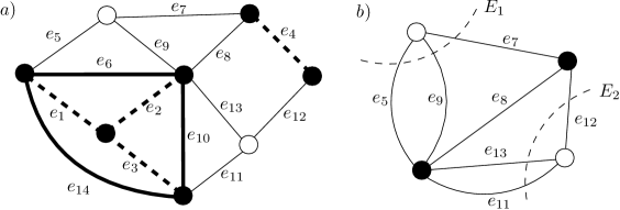
Figure 2: Illustration of Algorithm 2. The bold edges in (a) form a solution to Min-Max SI.

Now, we seek an independent set $I$ in $H$, i.e. a subset of the nodes of $H$ such that no two nodes in $I$ are incident in $H$. In Figure 2b the independent set contains two white nodes. Since $I$, $|I|=\ell$, is an independent set, the edge sets $E_{i}=\delta(i)$, $i\in[\ell]$, are disjoint and form an instance of the Min-Max RS problem with scenario set induced by $\mathcal{U}$. Notice that $\sum_{e\in\delta(i)}x^{*}_{e}\geq 1$ for each $i\in[\ell]$, which is guaranteed by the constraints (16). After normalization we get $\sum_{e\in\delta(i)}\hat{x}_{e}=1$ for each $i\in[\ell]$. So, $(\hat{x}_{e})_{e\in\delta(i)}$, $i\in[\ell]$, is a feasible solution to the relaxation of the Min-Max RS problem. Let $X$ be the set of edges chosen in Step 2.

Lemma 5.

The value of $\max_{\boldsymbol{\xi}\in\mathcal{U}}\sum_{e\in X}c_{e}^{\boldsymbol{\xi}}$ is $O(L^{*}\log K/\log\log K)$.

Proof.

Analogous to the proof of Lemma 3. ∎

Observe that $X$ contains exactly one edge from each $E_{i}$, $i\in I$. Because $I$ is an independent set, $F\cup X$ does not contain any cycle and thus $T=(V,F\cup X)$ is still a forest. We repeat the above construction in a number of rounds until $T$ is a spanning tree. Observe that after $k$ rounds the maximum cost of $T$ over $\mathcal{U}$ is $O(kL^{*}\log K/\log\log K)$. Hence, in order to obtain a desired approximation ratio we should give a bound on $k$.

1 Find $L^{*}$ and a feasible solution $\boldsymbol{x}^{*}=(x^{*}_{e})_{e\in E}$ to $\mathcal{LP}(L^{*})$ with the constraints (15)-(16);

2 foreach $e\in E$ with $x^{*}_{e}=0$ do $E\leftarrow E\setminus\{e\}$;

3 $\boldsymbol{x}\leftarrow\boldsymbol{x}^{*}$; let $T=(V,F)$, where $F\leftarrow\emptyset$;

Use Theorem 1 to transform solution $(x_{e})_{e\in E}$ into a solution $X$, $|X|=n-1$, for Min-Max SI ;

  // round 0

4 foreach $e\in X$ do

5       if $F\cup\{e\}$ does not contain a cycle then $F\leftarrow F\cup\{e\}$;

6      

7while $T$ is not tree  do // round $k$

8       Let $H=(U,W)$ be the graph obtained from $G$ by contracting every connected components of $T$ to a single node $u$ and $W\leftarrow\bigcup_{u\in U}\delta(u)$;

9       Find an independent set $I$ in $H$, $|I|=\ell$;

10       foreach $i\in I$ do

11             $E_{i}\leftarrow\delta(i)$;

12             foreach $e\in E_{i}$ do $\hat{x}_{e}\leftarrow x^{*}_{e}/(\sum_{e\in E_{i}}x^{*}_{e})$;

13            

14      Use Theorem 1 to transform $\hat{x}_{e}$, $e\in\bigcup_{i\in I}E_{i}$, into a solution $X$, $|X|=\ell$, for Min-Max RS;

15       foreach $e\in X$ do $F\leftarrow F\cup\{e\}$;

16      

return $T$

Algorithm 2 A deterministic algorithm for Min-Max ST

Lemma 6.

If an independent set $I$ found in graph $H=(U,W)$ is such that $|I|\geq|U|/\alpha$, where $\alpha>1$ is a constant. Then Algorithm 2 in $O(\log n)$ rounds yields to a spanning tree $T$.

Proof.

Let $C_{k}$ be the number of connected components in graph $T=(V,F)$ at the beginning of the $k$th round, $k=0,\ldots,\hat{k}$, where $\hat{k}$ is the last round in Algorithm 2. In the round 0, we compute a feasible solution $X_{0}$, $|X_{0}|=n-1$, for Min-Max SI and include in $F$ only the edges of $X_{0}$, which do not form a cycle in graph $T$. Hence

$$C_{1}\leq C_{0}-\frac{n-1}{3},\;C_{0}=n.$$ (17)

In the $k$th round, $k\in[\hat{k}]$, we find a independent set $I$ in graph $H=(U,W)$, with node set $U$ corresponding to shrunk connected components of $T$, $|U|=C_{k}$. We then choose a feasible solution $X_{k}$, $|X_{k}|=|I|$ for Min-Max RS and add the edges of $X_{k}$ to $F$. Since $|I|\geq C_{k}/\alpha$, we see that

$$C_{k+1}\leq C_{k}-C_{k}/\alpha=C_{k}(1-1/\alpha),\;k\in[\hat{k}].$$ (18)

From (17) and (18) it may be concluded that

$$C_{\hat{k}+1}\leq C_{\hat{k}}(1-1/\alpha)\leq C_{1}(1-1/\alpha)^{\hat{k}}\leq\frac{2n+1}{3}(1-1/\alpha)^{\hat{k}}.$$

As $C_{\hat{k}+1}=1$, we have $\hat{k}\leq\ln(\alpha/(\alpha-1))\ln((2n+1)/3)$, which proves the lemma. ∎

The assumption about finding an independent set $I$, such that $|I|\geq|U|/\alpha$ for some constant $\alpha>0$, is the crucial one. It determines the classes of graphs, for which Algorithm 2 runs in polynomial time. It is worth pointing out that the maximum independent set problem is hard to approximate within a factor of $|U|^{1-\epsilon}$ for any fixed $\epsilon>0$ unless P=NP [34]. Fortunately, we only need to find, in polynomial time, an independent set $I$ such that $|I|\geq|U|/\alpha$, where $\alpha>1$ is a constant. Let $\alpha(H)$ be an independence number of graph $H$, i.e. the size of the largest independent set in $H$. In [31] the following lower bound on $\alpha(H)$ was shown: $\alpha(H)\geq|U|/(1+\overline{d})$, where $\overline{d}$ denote the average node degree in $H$. The following simple heuristic, often called Algorithm MIN (see, e.g., [16]), finds an independent set $I$ of size at least $|U|/(1+\overline{d})$, namely: find node $i$ in $H$ of the minimum degree and add $i$ to a set $I$; delete $i$ and all its neighbors from $U$; continue adding such nodes to $I$ until all nodes of $U$ are exhausted. Now restricting to the graphs, in which $\overline{d}$ is bounded by a constant, i.e. the graphs of bounded average degree, we can satisfy the assumption of Lemma 6 with $\alpha=1+\overline{d}$ and obtain the algorithm which runs in polynomial time.

It is well-known that node coloring of and node independence in a graph are closely related. Namely, a subset of the nodes of the graph corresponding to a fixed color is independent. Accordingly, if graph $H$ is planar, then by the Four Color Theorem, we have $\alpha(H)\geq|U|/4$. This 4-coloring and the corresponding independent set $I\subset U$, $|I|\geq|U|/4$, can be computed in $O(|U|^{2})$ time [28] (if $H$ is additionally a triangle-free-graph, then Algorithm MIN, a much simpler than latter one, can be applied to find an independent set $I$ such that $|I|\geq|U|/4$, see [16]). In consequence, we can satisfy the assumption of Lemma 6 with $\alpha=4$. So, for graphs with bounded average degree or planar graphs there is a polynomial time implementation of Algorithm 2, in which the number of rounds is at most $O(\log n)$. We thus get the following result:

Theorem 3.

Let $G$ be a graph with average degree bounded or planar. Then there is a deterministic $O(\log n\log K/\log\log K)$-approximation algorithm for Min-Max ST.

4.2 A randomized approximation algorithm for the general case

We now propose a randomized $O(\log n)$-approximation algorithm for Min-Max ST, which can be applied to all graphs. We only have to make a mild assumption that $K=\textrm{poly}(n)$, similarly as in [5, 21, 20]. There is no loss of generality in assuming that $L^{*}=1$, and all the edge costs are such that $c^{\boldsymbol{\xi}}_{e}\in[0,1]$, $e\in E$, $\boldsymbol{\xi}\in\mathcal{U}$. We can easily meet this assumption by dividing all the edge costs by $L^{*}$.

Let $x$-coin be a coin which comes up head with probability $x\in(0,1]$. We use such a coin to transform the feasible fractional solution $\boldsymbol{x}^{*}$ into a feasible solution to Min-Max ST as follows (see Algorithm 3). We start with $T=(V,F)$, where $F=\emptyset$. Then for each edge $e\in E$, we simply flip an $x^{*}_{e}$-coin $\hat{k}$ times, where $\hat{k}$ will be specified later, and if it comes up heads at least once, then edge $e$ is included in $F$. If the resulting graph $T$ is connected, then a spanning tree of $T$ is returned. If $T$ is not connected, then the algorithm fails. We will show, however, that $T$ is connected with high probability.

1 Find $L^{*}$ and a feasible solution $\boldsymbol{x}^{*}=(x^{*}_{e})_{e\in E}$ to $\mathcal{LP}(L^{*})$ with the constraints (15)-(16);

2 foreach $e\in E$ with $x^{*}_{e}=0$ do $E\leftarrow E\setminus\{e\}$;

3 let $T=(V,F)$, where $F\leftarrow\emptyset$;

/* Randomized rounding */

$\hat{k}\leftarrow\lceil(40+\gamma)\ln n\rceil$ ;

  // $\gamma$ is a suitable constant

4 foreach $e\in E$ do  flip an $x^{*}_{e}$-coin $\hat{k}$ times, if it comes up heads at least once, then add $e$ to $F$;

5 if $T$ is connected then return a spanning tree of $T=(V,F)$ else fail;

 

Algorithm 3 A randomized algorithm for Min-Max ST

Let $\gamma$ be constant such that $\lceil(40+\gamma)\ln n\rceil>\ln(2n^{2}K)$. The existence of such a constant easily follows from the fact that $K=\textrm{poly}(n)$. The cost of a spanning tree constructed is established by the following lemma.

Lemma 7.

Let $F$ is a set of edges chosen in Algorithm 3. Then the probability that

$$\sum_{e\in F}c^{\boldsymbol{\xi}}_{e}>\hat{k}L^{*}+(\mathrm{e}-1)\sqrt{\hat{k}L^{*}\ln(2n^{2}K)},$$

under any scenario $\boldsymbol{\xi}\in\mathcal{U}$, is at most $\frac{1}{2n^{2}K}$, where $\hat{k}=\lceil(40+\gamma)\ln n\rceil$.

Proof.

Consider a random variable $\mathrm{X}_{e}$ such that $\mathrm{X}_{e}=1$ if edge $e$ is added to $F$; and $\mathrm{X}_{e}=0$ otherwise. Clearly, $\mathrm{Pr}[\mathrm{X}_{e}=1]=1-(1-x^{*}_{e})^{\hat{k}}$. Thus

$$\mathbf{E}\left[\sum_{e\in E}c^{\boldsymbol{\xi}}_{e}\mathrm{X}_{e}\right]=\sum_{e\in E}c^{\boldsymbol{\xi}}_{e}\mathrm{Pr}[\mathrm{X}_{e}=1]=\sum_{e\in E}c^{\boldsymbol{\xi}}_{e}(1-(1-x^{*}_{e})^{\hat{k}})\leq\hat{k}\sum_{e\in E}c^{\boldsymbol{\xi}}_{e}x^{*}_{e}\leq\hat{k}L^{*},$$ (19)

where the first inequality in (19) is due to the fact that $1-(1-x^{*}_{e})^{\hat{k}}\leq\hat{k}x^{*}_{e}$ for $\hat{k}\geq 1$ and $x^{*}_{e}\in(0,1]$. Let $\psi^{\boldsymbol{\xi}}$ be the event that $\sum_{e\in E}c^{\boldsymbol{\xi}}_{e}\mathrm{X}_{e}>\hat{k}L^{*}+(\mathrm{e}-1)\sqrt{\hat{k}L^{*}\ln(2n^{2}K)}$. Since the edge costs are such that $c^{\boldsymbol{\xi}}_{e}\in[0,1]$, $e\in E$, (19) and Chernoff-Hoeffding bound [27, Theorem 1 and inequality (1.13) for $D(\hat{k}L^{*},1/(2n^{2}K))$ under the assumption that $\hat{k}>\ln(2n^{2}K)$] and the equality $L^{*}=1$, show that

$$\mathrm{Pr}\left[\psi^{\boldsymbol{\xi}}\right]\leq\mathrm{Pr}\left[\sum_{e\in E}c^{\boldsymbol{\xi}}_{e}\mathrm{X}_{e}>\hat{k}L^{*}+(\mathrm{e}-1)\sqrt{\hat{k}L^{*}\ln(2n^{2}K)}\right]<\frac{1}{2n^{2}K},$$ (20)

which proves the lemma. ∎

We now estimate the probability of the event that the graph the graph $T=(V,F)$, built in Step 3 of Algorithm 3, is connected. In this case the solution returned is a spanning tree; otherwise the algorithm fails. Notice first that Step 3 can be seen as performing $\hat{k}$ rounds independently. Namely, in each round $k$, $k\in[\hat{k}]$, we flip an $x^{*}_{e}$-coin for each edge $e\in E$ and include $e$ in $F$ when it comes up head. The further analysis is adapted from [4]. Let $T_{k}$ be the graph obtained from $T_{k-1}$ after the $k$th round, $k\in[\hat{k}]$. Initially, $T_{0}$ has no edges. Let $C_{k}$ stands for the number of connected components of $T_{k}$. Obviously, $C_{0}=n$. We say that round $k$ is “successful” if either $C_{k-1}=1$ ($T_{k-1}$ is connected) or $C_{k}<0.9C_{k-1}$.

Lemma 8 (Alon [4]).

Assume that for every connected component $D$ of $T_{k-1}$, the sum of probabilities associated to edges from $E$ that connect nodes of $D$ to nodes outside $D$ is at least 1. Then for every $k$, the conditional probability that round $k$ is “successful”, given any set of components in $T_{k-1}$, is at least $1/2$.

Obviously, in our case the assumption of Lemma 8 is satisfied, which is due to the form of constraints (16) in the linear program $\mathcal{LP}(L)$.

Lemma 9.

Let $\mathcal{C}$ be the event that $C_{\hat{k}}\geq 2$ ($T_{\hat{k}}$ is not connected). Then $\mathrm{Pr}[\mathcal{C}]<\frac{1}{2n^{2}}$ provided that $\hat{k}=\lceil(40+\gamma)\ln n\rceil$.

Proof.

We now estimate the number $\ell$ of successful rounds, among $\hat{k}$ performed rounds, which are sufficient to ensure $C_{\hat{k}}=1$. We must have $(0.9)^{\ell}n<2$. The above inequality holds, in particular, when $\ell\geq 10\ln n$. Let $\mathrm{Z}_{k}$ be a binary random variable such that $\mathrm{Z}_{k}=1$ if and only if round $k$ is “successful”, $k\in\hat{k}$. In order to cope with the dependency of the events: round $k$ is “successful”, we estimate $\mathrm{Pr}[\sum_{k\in\hat{k}}\mathrm{Z}_{k}<10\ln n]$ from above by $\mathrm{Pr}[\mathrm{B}(\hat{k},1/2)<10\ln n]$, where $\mathrm{B}(\hat{k},1/2)$ is a binomial random variable (see Lemma 8 and [25, Lemma 14.6]). Thus applying Chernoff bound (see, e.g., [25, Corollary 4.10 for $\delta=1/2$] and $\hat{k}=\lceil(40+\gamma)\ln n\rceil$) we get the following upper bound on $\mathrm{Pr}[\mathcal{C}]$:

$$\mathrm{Pr}[\mathcal{C}]\leq\mathrm{Pr}\left[\sum_{k\in\hat{k}}\mathrm{Z}_{k}<10\ln n\right]<\mathrm{Pr}[\mathrm{B}(\hat{k},1/2)<10\ln n]\leq\mathrm{e}^{-(40+\gamma)\ln n/16}\leq\mathrm{e}^{-2.5\ln n}\leq\frac{1}{2n^{2}},$$ (21)

for each $n\geq 4$. This proves the lemma. ∎

Accordingly, the union bound gives $\Pr[\psi^{\boldsymbol{\xi}_{1}}\dots\cup\psi^{\boldsymbol{\xi}_{K}}\cup\mathcal{C}]<1/n^{2}$ (see Lemmas 7 and 9 and the inequalities (20) and (21)). Hence, after $\hat{k}=\lceil(40+\gamma)\ln n\rceil$ rounds, Algorithm 3 yields to a spanning tree of $T=(V,F)$ with the maximum cost over $\mathcal{U}$ of $O(\ln n+\ln K)L^{*}$ with probability at least $1-\frac{1}{n^{2}}$, where $L^{*}\leq OPT$ and $K=\textrm{poly}(n)$. We thus get the following theorem.

Theorem 4.

There is a randomized approximation algorithm for Min-Max ST that yields an $O(\log n)$-approximate solution with high probability.

5 Conclusions

There is still an open question concerning the Min-Max SP problem. For this problem, there exist an $O(\sqrt{n\log K/\log\log K})$-approximation algorithm, designed in this paper, and $O(\log^{1-\epsilon}K)$ lower bound on the approximability of the problem, known from literature. Accordingly, closing this gap is an interesting subject of further research. On the other hand, for the minmax version of the minimum assignment problem, which is closely related to Min-Max SP (there is a cost preserving reduction from Min-Max SP to the minmax assignment problem [2]) a LP-based randomized $\widetilde{O}(\sqrt{n})$-approximation algorithm, that produces a matching containing $n-o(n)$ edges, was proposed in [5]. Thus the factor of $\sqrt{n}$ appears in the approximation algorithms for both problems and removing it it seems to be unlikely.

Acknowledgements

This work was supported by the National Science Centre, Poland, grant 2017/25/B/ST6/00486.

Appendix A Some proofs

Proof of Proposition 1.

Consider an instance of Min-Max SP presented in Figure 3. We call arcs with zero costs under every scenario dummy arcs – see the dashed ones.

Figure 3: An instance of Min-Max SP with the integrality gap of at least 2.

We see at once that $x^{*}_{e_{i}}=1/2$, $i\in[4]$, $x^{*}_{f_{i}}=1/2$, $i\in[4]$, is a feasible solution to $\mathcal{LP}(1)$ with the constraints (12)-(13) and every integral solution for this instance has the maximum cost over $\mathcal{U}^{(0)}$ equal to 2. Hence the integrality gap of $\mathcal{LP}$ with (12)-(13) is at least 2.

We now gradually increase the gap. A new instance of Min-Max SP, i.e. graph $G^{(1)}=(V^{(1)},E^{(1)})$ with a scenario set $\mathcal{U}^{(1)}$, is build in the following way. We replace every arc $e_{i}$, $i\in[4]$, in $G^{(0)}$ (see Figure 3a) by the graph $G^{(0)}$, denoted by $G^{(0)}_{e_{i}}$, obtaining $G^{(1)}$, where $|E^{(1)}|=4|E^{(0)}|+4$, $|V^{(1)}|=4(|V^{(0)}|-2)+7$. Then we construct scenario set $\mathcal{U}^{(1)}$ as follows. We replace two values of 1 in every scenario $\boldsymbol{\xi}^{(0)}\in\mathcal{U}^{(0)}$ by two matrices $\mathbf{\Xi}^{(1)}_{1}$ and $\mathbf{\Xi}^{(1)}_{2}$ of the size $|E^{(0)}|\times|\mathcal{U}^{(0)}|^{2}$, respectively, where the columns of the matrices form the Cartesian product $\mathcal{U}^{(0)}\times\mathcal{U}^{(0)}$, i.e.

$$\left(\begin{array}[]{c}\mathbf{\Xi}^{(1)}_{1}\\ \mathbf{\Xi}^{(1)}_{2}\end{array}\right)=\left(\begin{array}[]{ccccccccccccc}\boldsymbol{\xi}^{(0)}_{1}&\boldsymbol{\xi}^{(0)}_{1}&\ldots&\boldsymbol{\xi}^{(0)}_{1}&\boldsymbol{\xi}^{(0)}_{2}&\boldsymbol{\xi}^{(0)}_{2}&\ldots&\boldsymbol{\xi}^{(0)}_{2}&\ldots&\boldsymbol{\xi}^{(0)}_{|\mathcal{U}^{(0)}|}&\boldsymbol{\xi}^{(0)}_{|\mathcal{U}^{(0)}|}&\ldots&\boldsymbol{\xi}^{(0)}_{|\mathcal{U}^{(0)}|}\\ \boldsymbol{\xi}^{(0)}_{1}&\boldsymbol{\xi}^{(0)}_{2}&\ldots&\boldsymbol{\xi}^{(0)}_{|\mathcal{U}^{(0)}|}&\boldsymbol{\xi}^{(0)}_{1}&\boldsymbol{\xi}^{(0)}_{2}&\ldots&\boldsymbol{\xi}^{(0)}_{|\mathcal{U}^{(0)}|}&\ldots&\boldsymbol{\xi}^{(0)}_{1}&\boldsymbol{\xi}^{(0)}_{2}&\ldots&\boldsymbol{\xi}^{(0)}_{|\mathcal{U}^{(0)}|}\end{array}\right).$$

Every value of 0 in $\boldsymbol{\xi}^{(0)}$ that corresponds to arc $e_{i}$, $i\in[4]$, is replaced by zero matrix $\mathbf{O}^{(1)}$ of the size $|E^{(0)}|\times|\mathcal{U}^{(0)}|^{2}$ and every value of 0 in $\boldsymbol{\xi}^{(0)}$ that corresponds to arc $f_{i}$, $i\in[4]$, is replaced by zero matrix $\boldsymbol{0}^{(1)}$ of the size $1\times|\mathcal{U}^{(0)}|^{2}$ (see Figure 3b). Thus $|\mathcal{U}^{(1)}|=|\mathcal{U}^{(0)}|^{2}|\mathcal{U}^{(0)}|$. The resulting instance is shown in Figure 4.

Figure 4: An instance of Min-Max SP with the integrality gap of at least 4

Note that every $s-t$ path in $G^{(1)}$ contains exactly four solid arcs. From the construction of $\mathcal{U}^{(1)}$ it follows that there exists a scenario in which the costs of these four arcs are equal to 1. It is the maximum cost, since each scenario $\boldsymbol{\xi}^{(1)}\in\mathcal{U}^{(1)}$ has exactly four 1’s. Accordingly, every integral solution for this instance has the maximum cost over $\mathcal{U}^{(1)}$ equal to 4. Let $\boldsymbol{x}^{*}\in(0,1]^{|E^{(1)}|}$ be given by $x^{*}_{e}=1/4$ for the solid arcs $e$ in $G^{(1)}$; $x^{*}_{f_{i}}=1/2$ for $i\in[4]$ and the components of $\boldsymbol{x}^{*}$ corresponding to the dashed arcs in $G^{(0)}_{e_{i}}$, $i\in[4]$, are equal to $1/4$. It is easy to check that $\boldsymbol{x}^{*}$ is feasible to $\mathcal{LP}(1)$. Therefore the integrality gap of $\mathcal{LP}$ with (12)-(13) is at least 4.

Repeated application of the above construction enables us to increase the integrality gap of at least 8. That is, we again replace each solid arc $e_{i}$, $i\in[4]$, in $G^{(0)}$ (see Figure 3a) by the graph $G^{(1)}$. This leads to graph $G^{(2)}$ with $|E^{(2)}|=4|E^{(1)}|+4$, $|V^{(2)}|=4(|V^{(1)}|-2)+7$. Then we built $\mathcal{U}^{(2)}$ as follows. We now replace two values of 1 in every scenario $\boldsymbol{\xi}^{(0)}\in\mathcal{U}^{(0)}$ by two matrices $\mathbf{\Xi}^{(2)}_{1}$ and $\mathbf{\Xi}^{(2)}_{2}$ of the size $|E^{(1)}|\times|\mathcal{U}^{(1)}|^{2}$, respectively, where the columns of the matrices form the Cartesian product $\mathcal{U}^{(1)}\times\mathcal{U}^{(1)}$:

$$\left(\begin{array}[]{c}\mathbf{\Xi}^{(2)}_{1}\\ \mathbf{\Xi}^{(2)}_{2}\end{array}\right)=\left(\begin{array}[]{ccccccccccccc}\boldsymbol{\xi}^{(1)}_{1}&\boldsymbol{\xi}^{(1)}_{1}&\ldots&\boldsymbol{\xi}^{(1)}_{1}&\boldsymbol{\xi}^{(1)}_{2}&\boldsymbol{\xi}^{(1)}_{2}&\ldots&\boldsymbol{\xi}^{(1)}_{2}&\ldots&\boldsymbol{\xi}^{(1)}_{|\mathcal{U}^{(1)}|}&\boldsymbol{\xi}^{(1)}_{|\mathcal{U}^{(1)}|}&\ldots&\boldsymbol{\xi}^{(1)}_{|\mathcal{U}^{(1)}|}\\ \boldsymbol{\xi}^{(1)}_{1}&\boldsymbol{\xi}^{(1)}_{2}&\ldots&\boldsymbol{\xi}^{(1)}_{|\mathcal{U}^{(1)}|}&\boldsymbol{\xi}^{(1)}_{1}&\boldsymbol{\xi}^{(1)}_{2}&\ldots&\boldsymbol{\xi}^{(1)}_{|\mathcal{U}^{(1)}|}&\ldots&\boldsymbol{\xi}^{(1)}_{1}&\boldsymbol{\xi}^{(1)}_{2}&\ldots&\boldsymbol{\xi}^{(1)}_{|\mathcal{U}^{(1)}|}\end{array}\right),\;\boldsymbol{\xi}^{(1)}\in\mathcal{U}^{(1)}.$$

Every 0 in $\boldsymbol{\xi}^{(0)}$ that corresponds to arc $e_{i}$, $i\in[4]$, is replaced by matrix $\mathbf{O}^{(2)}$ of the size $|E^{(1)}|\times|\mathcal{U}^{(1)}|^{2}$ and every 0 in $\boldsymbol{\xi}^{(0)}$ that corresponds to arc $f_{i}$, $i\in[4]$, is replaced by matrix $\boldsymbol{0}^{(2)}$ of the size $1\times|\mathcal{U}^{(1)}|^{2}$ and so $|\mathcal{U}^{(2)}|=|\mathcal{U}^{(1)}|^{2}|\mathcal{U}^{(0)}|$.

The proof of the proposition is based on repeating the above construction $r$ times. We get graph $G^{(r)}=(V^{(r}),E^{(r}))$, where $|E^{(r)}|=4|E^{(r-1)}|+4$, $|V^{(r)}|=4(|V^{(r-1)}|-2)+7$, and scenario set $\mathcal{U}^{(r)}$ with the cardinality of $|\mathcal{U}^{(r-1)}|^{2}|\mathcal{U}^{(0)}|$. Now, the integrality gap of $\mathcal{LP}$ with (12)-(13) for the resulting instance is at least $2^{r+1}$. Set $k=2^{r+1}$, $K=|\mathcal{U}^{(r)}|$, $m=|E^{(r)}|$ and $n=|V^{(r)}|$. Since $|\mathcal{U}^{(0)}|=4$, $|E^{(0)}|=8$ and $|V^{(0)}|=7$, a trivial verification yields $K=4^{2^{r+1}-1}=4^{k-1}$, $m=4^{r+1}+\sum_{p=1}^{r+1}4^{p}=\frac{7}{3}k^{2}-\frac{4}{3}$ and $n=2+5\sum_{p=0}^{r}4^{p}=2+\frac{5}{3}(k^{2}-1)$. The latter ones show that $\mathcal{LP}(L)$ with (12)-(13) has an integrality gap of at least $\Omega(\sqrt{n})$, which completes the proof. ∎

Proof of Proposition 2.

Figure 5: An instance of Min-Max MST

Given any integer $k>0$. A construction of an instance of Min-Max MST is as follows: graph $G=(V,E)$ is a series composition of $k$, $2k$-edge subgraphs, $G^{(1)},\ldots,G^{(k)}$ (see the graph depicted in Figure 5). Thus $m=2k^{2}$ and $n=k^{2}+k+1$ ($\sqrt{n}=\Theta(k)$). In order to form a scenario set $\mathcal{U}$, we define the Cartesian product $\mathcal{E}=\prod_{i=1}^{k}\{e^{(i)}_{1},\ldots,e^{(i)}_{k}\}$ that corresponds to the solid edges of subgraph $G^{(i)}$, $i\in[k]$. Each $k$-tuple $(e^{(1)},\ldots,e^{(k)})\in\mathcal{E}$ determines a cost scenario $\boldsymbol{\xi}\in\mathcal{U}$. Namely, $c^{\boldsymbol{\xi}}_{e^{(i)}}=1$ for $i\in[k]$; the costs of the rest of the edges, $E\setminus\{e^{(1)},\ldots,e^{(k)}\}$, are equal to zero under $\boldsymbol{\xi}$. Hence $K=|\mathcal{U}|=k^{k}$. Let $\boldsymbol{x}^{*}\in(0,1]^{m}$ be given by $x^{*}_{e^{(i)}_{j}}=1/k$ for $i,j\in[k]$ (the solid edges) and the components of $\boldsymbol{x}^{*}$ corresponding to the dashed edges are equal to 1. An easy computation shows that: $\sum_{e\in E}c^{\boldsymbol{\xi}}_{e}x^{*}_{e}=1$ for every $\boldsymbol{\xi}\in\mathcal{U}$, $\sum_{e\in E}x^{*}_{e}=k^{2}+k=n-1$. Observe that the constraints: $\sum_{e\in\delta(S)}x^{*}_{e}\geq 1$ for every $\emptyset\not=S\subset V$ are also fulfilled, since from every node emanates a dashed edge except for the leftmost node, say $s$, – in this case $\sum_{e\in\delta(s)}x^{*}_{e}=1$. Accordingly, $\boldsymbol{x}^{*}$ is a feasible solution to $\mathcal{LP}(1)$ with the constraints (15)-(16). From the construction of $\mathcal{U}$ it follows that every integer solution for the instance build has the maximum cost over $\mathcal{U}$ equal to $k$. This leads to the integrality gap of the instance of at least $k$. If we prove that $k=\Omega(\log{K}/\log{\log{K}})$, the assertion follows. Indeed, $\log{K}=k\log{k}$, $\log{K}/\log\log{K}=k\log{k}/(\log{k}+\log{\log{k}})=\Theta(k)$. ∎

References

- [1] R. K. Ahuja, T. L. Magnanti, and J. B. Orlin. Network Flows: theory, algorithms, and applications. Prentice Hall, Englewood Cliffs, New Jersey, 1993.
- [2] H. Aissi, C. Bazgan, and D. Vanderpooten. Complexity of the min-max and min-max regret assignment problems. Operations Research Letters, 33:634–640, 2005.
- [3] H. Aissi, C. Bazgan, and D. Vanderpooten. Min-max and min-max regret versions of combinatorial optimization problems: a survey. European Journal of Operational Research, 197:427–438, 2009.
- [4] N. Alon. A note on network reliability. In D. Aldous, P. Diaconis, J. Spencer, and J. M. Steele, editors, Discrete Probability and Algorithms, volume 72 of IMA Volumes in Mathematics and its applications, pages 11–14. Springer-Verlag, 1995.
- [5] S. Arora, A. Frieze, and H. Kaplan. A new rounding procedure for the assignment problem with applications to dense graph arrangement problems. Mathematical Programming, 92:1–36, 2002.
- [6] I. Averbakh. On the complexity of a class of combinatorial optimization problems with uncertainty. Mathematical Programming, 90:263–272, 2001.
- [7] A. Ben-Tal, L. El Ghaoui, and A. Nemirovski. Robust optimization. Princeton Series in Applied Mathematics. Princeton University Press, Princeton, NJ, 2009.
- [8] V. Bilò, V. Goya, R. Ravi, and M. Singh. On the Crossing Spanning Tree Problem. In APPROX 2004, pages 51–60. Springer-Verlag, 2004.
- [9] C. Büsing. Recoverable robust shortest path problems. Networks, 59:181–189, 2012.
- [10] V. G. Deineko and G. J. Woeginger. Complexity and in-approximability of a selection problem in robust optimization. 4OR - A Quarterly Journal of Operations Research, 11:249–252, 2013.
- [11] B. Doerr. Improved approximation algorithms for the Min-Max selecting Items problem. Information Processing Letters, 113:747–749, 2013.
- [12] A. Dolgui and S. Kovalev. Min-max and min-max (relative) regret approaches to representatives selection problem. 4OR - A Quarterly Journal of Operations Research, 10:181–192, 2012.
- [13] M. Ehrgott. Multicriteria optimization. Springer, 2005.
- [14] M. Ehrgott and X. Gandibleux. A survey and annoted bibliography of multiobjective combinatorial optimization. OR Spectrum, 22:425–460, 2000.
- [15] F. Grandoni, R. Ravi, M. Singh, and R. Zenklusen. New approaches to multi-objective optimization. Mathematical Programming, 146:525–554, 2014.
- [16] J. R. Griggs. Lower Bounds on the Independence Number in Terms of the Degrees. Journal of Combinatorial Theory, Series B, 34:22–39, 1983.
- [17] P. Kall and S. W. Wallace. Stochastic Programming. John Wiley and Sons, 1994.
- [18] A. Kasperski, A. Kurpisz, and P. Zieliński. Approximating the min-max (regret) selecting items problem. Information Processing Letters, 113:23–29, 2013.
- [19] A. Kasperski, A. Kurpisz, and P. Zieliński. Approximability of the robust representatives selection problem. Operations Research Letters, 43:16–19, 2015.
- [20] A. Kasperski and P. Zieliński. On the approximability of robust spanning problems. Theoretical Computer Science, 412:365–374, 2011.
- [21] I. Katriel, C. Kenyon-Mathieu, and E. Upfal. Commitment under uncertainty: two-stage matching problems. Theoretical Computer Science, 408:213–223, 2008.
- [22] P. Kouvelis and G. Yu. Robust Discrete Optimization and its Applications. Kluwer Academic Publishers, 1997.
- [23] C. Liebchen, M. E. Lübbecke, R. H. Möhring, and S. Stiller. The concept of recoverable robustness, linear programming recovery, and railway applications. In Robust and Online Large-Scale Optimization, volume 5868 of Lecture Notes in Computer Science, pages 1–27. Springer-Verlag, 2009.
- [24] T. L. Magnanti and L. A. Wolsey. Optimal Trees. In M. O. Ball, T. L. Magnanti, C. L. Monma, and G. L. Nemhauser, editors, Network Models, Handbook in Operations Research and Management Science, volume 7, pages 503–615. North-Holland, Amsterdam, 1995.
- [25] M. Mitzenmacher and E. Upfal. Probability and Computing: Randomized Algorithms and Probabilistic Analysis. Cambridge University Press, 2005.
- [26] C. H. Papadimitriou and M. Yannakakis. On the approximability of trade-offs and optimal access of web sources. In FOCS, pages 86–92. IEEE Computer Society, 2000.
- [27] P. Raghavan. Probabilistic Construction of Deterministic Algorithms: Approximating Packing Integer Programs. Journal of Computer and System Sciences, 37:130–143, 1988.
- [28] N. Robertson, D. Sanders, and P. Seymour. The Four-Colour Theorem. Journal of Combinatorial Theory, Series B, 70:2–44, 1997.
- [29] R. T. Rockafellar and R. J.-B. Wets. Scenarios and Policy Aggregation in Optimization Under Uncertainty. Mathematics of Operations Research, 16:119–147, 1991.
- [30] E. Ulungu and J. Teghem. Multi-objective combinatorial optimization problems: A survey. Journal of Multi-criteria Decision Analysis, pages 83–104, 1994.
- [31] V. K. Wei. A lower bound on the stability number of a simple graph. Technical Memorandum 81-11217-9, Bell Laboratories, Murray Hill, NJ, 1981.
- [32] R. J.-B. Wets. The aggregation principle in scenario analysis and stochastic optimization. In S. W. Wallace, editor, Algorithms and Model Formulations in Mathematical Programming, pages 91–113. Springer-Verlag, 1989.
- [33] D. P. Williamson and D. B. Shmoys. The Design of Approximation Algorithms. Cambridge University Press, 2010.
- [34] D. Zuckerman. Linear Degree Extractors and the Inapproximability of Max Clique and Chromatic Number. Theory of Computing, 3:103–128, 2007.